Attention Is Not What You Need: Revisiting Multi-Instance Learning for Whole Slide Image Classification

Abstract

Although attention-based multi-instance learning algorithms have achieved impressive performances on slide-level whole slide image (WSI) classification tasks, they are prone to mistakenly focus on irrelevant patterns such as staining conditions and tissue morphology, leading to incorrect patch-level predictions and unreliable interpretability. Moreover, these attention-based MIL algorithms tend to focus on salient instances and struggle to recognize hard-to-classify instances. In this paper, we first demonstrate that attention-based WSI classification methods do not adhere to the standard MIL assumptions. From the standard MIL assumptions, we propose a surprisingly simple yet effective instance-based MIL method for WSI classification (FocusMIL) based on max-pooling and forward amortized variational inference. We argue that synergizing the standard MIL assumption with variational inference encourages the model to focus on tumour morphology instead of spurious correlations. Our experimental evaluations show that FocusMIL significantly outperforms the baselines in patch-level classification tasks on the Camelyon16 and TCGA-NSCLC benchmarks. Visualization results show that our method also achieves better classification boundaries for identifying hard instances and mitigates the effect of spurious correlations between bags and labels.

1 Introduction

Whole slide images (WSIs) analysis has been widely utilized in clinical applications such as computer-aided tumour diagnosis and prognosis (Lu et al. 2021; Yao et al. 2020; Chen et al. 2021; Li, Li, and Eliceiri 2021). As a single WSI often contains billions of pixels and obtaining patch-level annotations is labour-intensive (Lu et al. 2021), it is a standard practice to crop the WSI into smaller patches and utilize Multi-Instance Learning (MIL) for classification. Multi-Instance Learning (MIL) is a weakly-supervised learning paradigm designed to learn from samples represented as bags (slides) of instances (patches). As computer-aided diagnosis models need to provide both slide-level and patch-level predictions of tumour tissues, MIL is particularly well-suited. (Li, Li, and Eliceiri 2021; Qu et al. 2022).

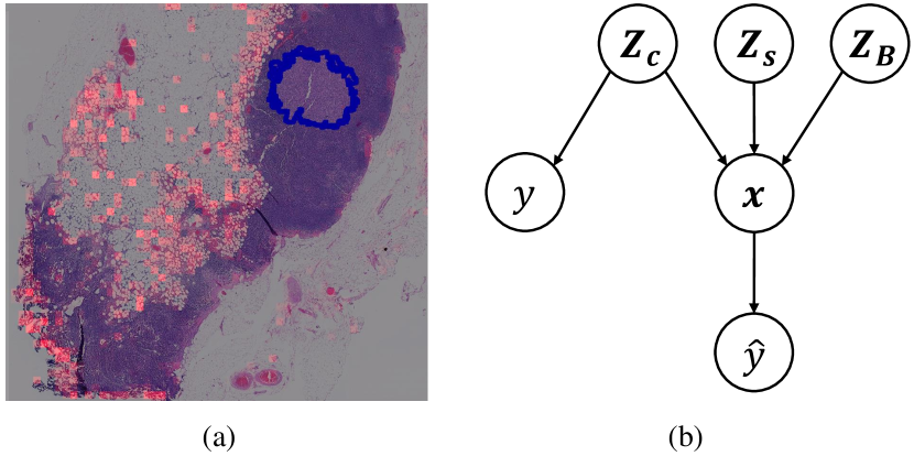
Figure 1: (a) MIL algorithms based on attention may produce incorrect patch-level attention map with correct slide-level prediction. (b) A causal graph for the generative procedure of patches and their labels.

Most existing MIL-based WSI classification algorithms focus on slide-level predictions and utilize attention (Vaswani et al. 2017) for aggregating patch-level representations into slide-level (Ilse, Tomczak, and Welling 2018; Li, Li, and Eliceiri 2021; Shao et al. 2021; Qu et al. 2022; Zhang et al. 2022a, 2023; Tang et al. 2023, 2024; Keum et al. 2024). Generally speaking, these algorithms utilize the attention mechanism to assign weights for each instance within a bag and aggregate their weighted representations for classification. However, many attention-based MIL methods deviate from the standard MIL assumption, which can limit their interpretability and trustworthiness in medical diagnosis (Raff and Holt 2023).

The standard MIL assumption states that a multi-instance bag is positive if and only if at least one of its instances is positive (Foulds and Frank 2010; Dietterich, Lathrop, and Lozano-Pérez 1997), which naturally aligns with the goal of WSI classification: a slide should be labelled as cancerous if and only if it contains at least one cancerous patch. Unfortunately, attention-based MIL algorithms do not pose additional constraints to enforce the standard MIL assumption when aggregating the attention weights. As a result, these models can sometimes misinterpret non-causal or irrelevant instances as influential, leading to less accurate and less interpretable predictions in medical diagnoses.

Another desideratum of WSI classification is that models should base their patch-level predictions on factors causally related to the tumour cells rather than spurious correlations. Fig. 1(b) illustrates the causal structure underlying the generation process of a patch $\bm{x}$, its ground-truth label $y$, and its predicted label $\hat{y}$. Three sets of factors determine the features of a patch: $\bm{Z}_{c}$, which causally influence whether a cell is cancerous, such as cellular morphology; $\bm{Z}_{s}$, which dictate stylistic elements, such as the positioning, size, and compression state of cells within the patch; and $\bm{Z}_{B}$, which are derived from the whole slide, including hematoxylin and eosin staining biases and tissue structures. Although an ideal model should make predictions based on $\bm{Z}_{c}$, most current models do not distinguish between $\bm{Z}_{c}$ and $\bm{Z}_{B}$.

Attention-based MIL methods do not enforce the standard multi-instance assumption or the causal relationship between patch-level and slide-level labels. First, as illustrated in Figure 1(a), higher attention scores can be assigned to regions that are irrelevant to the tumour, significantly diminishing the interpretability of assistive clinical diagnostics (Lin et al. 2023). Second, the models may struggle to identify tumour cells (hard instances) that are morphologically similar to normal cells and less malignant (Jögi et al. 2012; Zhang et al. 2023; Tang et al. 2023), leading to missed diagnoses in early-stage cancer patients. This is because attention-based models excessively prioritize salient instances (Tang et al. 2023; Zhang et al. 2023) and tend to exploit spurious correlations to fit the more challenging slides during training.

This paper studies the weakly supervised WSI classification problem without relying on the attention mechanism and proposes a simple yet effective instance-based MIL method: FocusMIL. Our approach focuses on the causal factors $\bm{Z}_{c}$ for predicting the label of instances while ignoring non-causal factors such as stylistic elements $\bm{Z}_{s}$ and bag-inherited information $\bm{Z}_{B}$. FocusMIL comprises a feed-forward neural network, reparameterization operations, and max-pooling. We emphasize that respecting the multi-instance assumption inherently constrains the model to classify based on tumour morphology $\bm{Z}_{c}$. The key distinction of our method from traditional max-pooling-based MIL classification methods is that we use mini-batch gradient decent with a batch size greater than one instead of SGD with a batch size of one. We discuss how a larger batch size enables the model to build better classification boundaries for recognizing hard instances and contributes to a more stable and efficient disentangling of $\bm{Z}_{c}$ and $\bm{Z}_{B}$.

Results on the Camelyon16 and TCGA-NSCLC datasets show that our approach significantly outperforms existing baselines at patch-level classification tasks and performs comparably with baselines on the slide level. Using slide-level supervision, our patch-level predictions predict salient and hard instances more accurately than existing methods. Furthermore, we designed a semi-synthetic dataset to test whether mainstream WSI classification algorithms respect the standard MIL assumptions and the results indicate that all the tested bag-level MIL methods failed this test. The code can be accessed from the supplementary material, which will be made publicly available after publication.

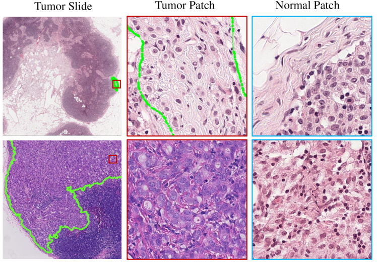
Figure 2: Comparison of tumour patches from different tumour slides and normal patches. Tumour cells from slides with small cancerous areas closely resemble normal cells. Conversely, tumour cells from slides with large cancerous areas exhibit very distinct tumour characteristics. Images are from Camelyon16 dataset.

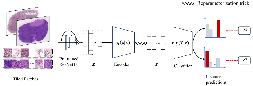
Figure 3: Overview of our FocusMIL with 2 slides in a mini-batch for illustration. Features are extracted from patches using a pre-trained feature extractor. The instance features are encoded into latent representations via a variational encoder. The classifier $P(Y|\bm{z})$ uses the inferred latent representations $\boldsymbol{z}$ to obtain patch-level prediction scores. Max-pooling is applied to the instance predictions of each MIL bag to derive the slide-level prediction.

2 Related Work

2.1 Attention-based MIL for WSI classification

Most MIL-based WSI classification algorithms aggregate patch-level features into bag-level features according to their attention scores. An early bag-based method, ABMIL (Ilse, Tomczak, and Welling 2018), utilizes a trainable network to calculate the attention scores of instance features for bag-level classification and obtains a bag-level representation through their weighted sum. Subsequent methods have inherited similar ideas and extensively incorporated various attention mechanisms (Li, Li, and Eliceiri 2021; Lu et al. 2021; Shao et al. 2021; Zhang et al. 2022a).

Attention-based MIL methods face the challenge of overfitting from three sources (Zhang et al. 2022a; Lin et al. 2023; Tang et al. 2023; Zhang et al. 2023). Firstly, many cancerous slides contain salient instances, i.e., areas with highly differentiated cancer cells that significantly differ from the normal ones (Qu et al. 2024; Jögi et al. 2012). Secondly, other slides may have hard instances, e.g., small cancerous areas where the cancer cells closely resemble normal cells (Bejnordi et al. 2017). Thirdly, the digital scanning equipment, slide preparation, and staining processes often introduce staining bias into WSI datasets (Zhang et al. 2022c). Existing studies (Tang et al. 2023; Zhang et al. 2023; Keum et al. 2024) have indicated that attention-based WSI classification methods may excessively focus on salient instances and fail to identify hard instances. For positive slides containing only hard instances, these methods often rely on spurious correlations caused by staining bias to fit the training set (Lin et al. 2023). Recent methods like WENO (Qu et al. 2022), MHIM (Tang et al. 2023), IBMIL (Lin et al. 2023), ACMIL (Zhang et al. 2023) and Slot-MIL (Keum et al. 2024) try to mitigate these problems; however, their generalization capability and patch-level classification performances are still not ideal.

2.2 Reproducibility in Multiple Instance Learning

Recent studies (Raff and Holt 2023) have shown that many widely used MIL methods, such as MI-Net (Wang et al. 2018) and TransMIL (Shao et al. 2021), do not adhere to the standard MIL assumptions and may leverage inductive biases, such as the absence of certain instances, as signals for predicting positive bags. As staining bias is prevalent in WSI analysis (Lin et al. 2023; Zhang et al. 2022c), models that do not respect the standard MIL assumptions can learn to use these spurious correlations (Raff and Holt 2023).

mi-Net (Zhou and Zhang 2002; Wang et al. 2018), and the recently proposed CausalMIL (Zhang et al. 2022b) are perhaps the only two methods that respect the MIL assumptions. CausalMIL applies a variational autoencoder (Kingma and Welling 2013) to the MIL problem, using a non-factorized prior distribution conditioned on bag information to provide a theoretical guarantee for identifying latent causal representation. However, mi-Net does not perform optimally in WSI classification, and CausalMIL has not yet been studied for WSI classification.

3 Method

3.1 Preliminaries

A WSI dataset with $n$ slides are treated as MIL bags $\mathcal{B}=\{\mathbf{B}_{1},\cdots,\mathbf{B}_{i},\cdots,\mathbf{B}_{n}\}$, where each slide has a slide-level label $Y_{i}\in\{0,1\}$ during training. Each slide is then cropped into patches corresponding to MIL instances $\mathbf{B}_{i}=\{\boldsymbol{p}_{i1},\cdots,\boldsymbol{p}_{ij},\cdots,\boldsymbol{p}_{in_{i}}\}$, where $n_{i}$ is the number of patches in the slide. For each patch $\boldsymbol{p}_{ij}$, there exists a patch-level label $y_{ij}\in\{0,1\}$ that is unknown to the learner. The standard multi-instance assumption states that a bag is positive if and only if at least one of its instances is positive:

$$Y_{i}=\begin{cases}0,&\text{if }\sum_{j}y_{i,j}=0,\\ 1,&\text{else},\end{cases}$$ (1)

which is equivalent to using max-pooling on the instances within a bag:

$$Y_{i}=\max_{j}\{y_{i,j}\}.$$ (2)

Given a feature extractor $f$, each instance is projected onto a $d$-dimensional feature vector $\boldsymbol{x}_{ij}=f(\boldsymbol{p}_{ij})\in\mathbb{R}^{d\times 1}$.

3.2 FocusMIL

Our main goal is to train a patch-level classifier from slide-level supervision while maintaining the standard multi-instance learning assumption and focusing on the causal factor $\bm{Z}_{c}$ that is invariant across slides. Formally, we assume

Assumption 1

The mechanism of determining whether a cell is cancerous from the causal factor $\bm{Z}_{c}$ in patches is invariant across slides.

Corresponding to Assumption 1, $\bm{Z}_{s}$ varies between different patches, while $\bm{Z}_{B}$ varies between different slides.

Our proposed FocusMIL method encapsulates the two desiderata of WSI classification within weakly supervised variational inference, as shown in Figure 3. Firstly, raw input patches $\bm{p}$ are processed with pre-trained feature extractors into $\bm{x}$. Then, the encoder encodes $\bm{x}$ into low-dimensional latent variables $\bm{z}$, which is used for predicting the patch labels. The predicted patch labels are pooled with the max-pooling operation to comply with the standard MIL assumption. It is noteworthy that the max-pooling operation and the calculation of the loss function are conducted once per slide, and the encoder and classifier are optimized for the total loss of multiple bags within the mini-batch. This is fundamentally different from most attention-based WSI algorithms, where the optimization is restricted to one slide per epoch.

The Importance of the Standard MIL Assumption

Models that respect the MIL assumptions predict bag labels solely based on the positive concept, e.g., the presence of tumour cells  (Foulds and Frank 2010; Dietterich, Lathrop, and Lozano-Pérez 1997). The two existing models that respect the MIL assumptions, mi-Net and CausalMIL, both use max pooling that aligns with the MIL problem setup. We argue that max-pooling effectively focuses the model on the causal factor $\bm{Z}_{c}$ for predicting the instance label. Due to the constraints of max-pooling, the model must base the bag label prediction solely on the most positive instance in the bag. If the classifier were to use $\bm{Z}_{B}$ to determine the instance label, because the bag-inherited information, such as staining conditions, is not entirely consistent across positive slides and differs on negative slides, the model would completely fail to fit the training set completely. Therefore, models that follow the MIL assumption must learn features such as the morphological structure of tumour cells, $\bm{Z}_{c}$, to fit the training set. A significant advantage is that models respecting MIL assumptions fitted well on the training set will achieve better patch-level classification results.

Mini-Batch Gradient Descent for WSI Classification

For WSI classification, the morphology of tumour cells may be different across slides due to the varying malignancy levels of cancer in patients (Zhang et al. 2023; Qu et al. 2024; Jögi et al. 2012). As shown in Figure 2, some slides contain large tumour areas with significant morphological differences from normal cells. In contrast, other slides have smaller tumour areas where the tumour cells have higher differentiation and less pronounced differences from normal cells (Qu et al. 2024), which are referred to as “hard instances” in some literature (Tang et al. 2023). When multiple bags are in the mini-batch, the encoder and classifier will forward propagate multiple bags simultaneously. To ensure the model can accurately predict slides with different degrees of cancerous malignancy within the batch, the optimization process must consider the features of both salient and hard instances, thereby learning a better classification boundary. Consider the following scenario: if the model established a classification boundary based only on salient instances, it would not be able to accurately classify slides of lower malignancy, resulting in a high loss.

Batch size $>1$ also contributes to the disentanglement of $\bm{Z}_{c}$ and $\bm{Z}_{B}$. Staining conditions vary across slides. When faced with tumour cells of different colours (e.g., tumour cell patch stained purple and tumour cell patch stained pink), the model can only rely on $\bm{Z}_{c}$ for prediction. If it depends on the staining information $\bm{Z}_{B}$ inherited from the slide, it will not be able to achieve accurate predictions (Zhang et al. 2022b).

Forward Armotized Variational Inference

Max-pooling and batch optimization alone are insufficient for WSI classification. This is evident from the performance of a batched version of the classical mi-Net (Wang et al. 2018). mi-Net often correctly classifies the bag but fails to classify its patches during training. Furthermore, both bag and patch classification frequently fail entirely on the testing set.

We argue that this is because mi-Net, due to the flexibility of neural networks, may learn extremely complex decision surfaces that overfit the training data (Raff and Holt 2023) and fail to effectively learn latent causal representations.

We employ a variational inference with forward KL divergence $\bm{z}$ to address this issue. Specifically,

$$D_{KL}[p(\bm{x},\bm{z})||q(\bm{x},\bm{z})]= \mathbb{E}_{p(\bm{x},\bm{z})}[\log\frac{p(\bm{x},\bm{z})}{k(\bm{x})}]$$

$$-\mathbb{E}_{p(\bm{x},\bm{z})}[\log q(\bm{z}|\bm{x})],$$ (3)

where $k(\bm{x})$ is a resampled distribution of the patches (Ambrogioni et al. 2019). As only the second term depends on the variational distribution, optimizing the forward KL divergence is equivalent to optimizing

$$\mathcal{L}_{KL}=-\mathbb{E}_{p(\bm{x},\bm{z})}[\log q(\bm{z}|\bm{x})].$$ (4)

The computation of the gradient in Equation 4 is straightforward as the expectation is defined for $p$ while the gradient is taken with respect to $q$.

For simplicity, we set the prior distribution as $p(\bm{z})=\mathcal{N}(0,\bm{I})$ and restrict the posterior as a factorized Gaussian encoder. Finally, the optimization objective can be obtained as:

$$\mathcal{L}= \ \log p(Y\mid\boldsymbol{z}^{*})-\mathbb{E}_{p(\bm{x},\bm{z})}\left[\log q(\boldsymbol{z}^{*}\mid\boldsymbol{x}^{*})\right]$$

$$\ -\beta\cdot\mathbb{E}_{q(\bm{z}|\bm{x})}\left[\log\frac{q(\boldsymbol{z}^{*}\mid\boldsymbol{x}^{*})}{p(\boldsymbol{z}^{*})}\right],$$ (5)

where $\beta$ is a hyperparameter for balancing the classifier and variational loss, $\boldsymbol{z}^{*}$ corresponds to the most positive latent representation of a bag obtained with max-pooling with respect to $p(Y|\bm{z}^{*})$, and $\boldsymbol{x}^{*}$ corresponds to the original feature of $\bm{z}^{*}$. A noteworthy fundamental difference from CausalMIL (Zhang et al. 2022b) is that the utilization of forward KL entirely eliminates the need to optimize a decoder $p(\bm{x}|\bm{z})$, which is unnecessary for WSI classification.

4 Experiments

4.1 Datasets, Metrics, and Baselines

Camelyon16 dataset is widely used for metastasis detection in breast cancer (Bejnordi et al. 2017). The dataset consists of 270 training and 129 testing WSIs, which yield roughly 2.7 million patches at 10× magnification (the second level in multi-resolution pyramid). Pixel-level labels are available for tumour slides. Every WSI is cropped into $256\times 256$ patches without overlap, and background patches are discarded. A patch is labeled positive if it contains $25\%$ or more cancer areas. The numbers of tumorous versus normal patches are imbalanced as the positive patch ratios of positive slide in the training and testing sets of Camelyon16 are approximately 8.8% and 12.7%, respectively.
TCGA-NSCLC includes two subtypes of lung cancer: Lung Adenocarcinoma (LUAD) and Lung Squamous Cell Carcinoma (LUSC), with a total of 1,054 diagnostic digital slides. Only slide-level labels are available for this dataset. We directly used the patches released by Li et al. (Li, Li, and Eliceiri 2021).

Semi-Synthetic Dataset

To test whether existing WSI classification methods respect the standard MIL assumption, we propose the Camelyon16 Standard-MIL test dataset, inspired by the ideas in (Raff and Holt 2023). Specifically, in the training set, we introduce poison by randomly selecting $20\%$ of the patches in the normal slides and increasing the intensity of their green channel. In the test set, we randomly select $20\%$ of the patches in tumour slides to introduce poison in the same way. A MIL model cannot legally learn to use the poison signal because it occurs only in normal slides (Raff and Holt 2023). If a model has a training AUC $>0.5$, but a test AUC $<0.5$, it relies on poison for prediction and does not respect the MIL assumption.

Evaluation Metrics

Due to the high level of class imbalance at the patch level, we report Area Under the Precision-Recall Curve (AUCPR) and F1 score for evaluation. For slide-level classification, we report AUC and Accuracy as the tumour and normal classes are balanced.

Baselines

We compare our method with recently published baselines, including ABMIL (Ilse, Tomczak, and Welling 2018), DSMIL (Li, Li, and Eliceiri 2021), TransMIL (Shao et al. 2021), DFTD-MIL (Zhang et al. 2022a), IBMIL (Lin et al. 2023), and CausalMIL (Zhang et al. 2022b). The first five methods are based on attention mechanisms, while CausalMIL is an instance-based method which has not been previously applied to WSI classification, to the best of our knowledge. For the Camelyon16, TCGA-NSCLC, and Camelyon16 Standard-MIL test datasets, we used a ResNet-18 (He et al. 2016) pretrained on ImageNet (Deng et al. 2009) to extract features. In addition, we also use features extracted by the powerful CTransPath (Wang et al. 2022) for the Camelyon16 dataset to conduct a more comprehensive comparison of various MIL methods.

4.2 Implementation details

The encoder of FocusMIL consists of a neural network with one hidden layer, with ReLU as the activation function. We use AdamW optimizer with an initial learning rate of $1\times 10^{-4}$ to update the model weights during the training. The dimension of the latent factor is set to 35. The mini-batch size for training FocusMIL model is 3.

For slide-level prediction, we apply max-pooling and mean-pooling to aggregate instance prediction scores for the Camelyon16 and TCGA-NSCLC datasets, respectively.

For the attention-based methods, we built other models based on their officially released codes and conducted grid searches for key hyperparameters. For CausalMIL (Zhang et al. 2022b), both its encoder and decoder are set up as neural networks with hidden layer neurons 128 and two other fully-connected layers are used to carve factorized prior distribution conditioned on the bag information. All the experiments are conducted with a Nvidia RTX4090 GPU. For more details, please refer to our code in the supplementary.

Table 1: Performance Comparison of MIL Methods using Resnet-18 and CTransPath Features. The subscripts are the corresponding $95\%$ confidence intervals. The most superior performance is highlighted in bold, while the second-best performance is indicated by underlining.

		Slide-level		Patch-level
		AUC	ACC	AUCPR	F1-score
ResNet-18 ImageNet pretrained	ABMIL	0.8052 (CI: 0.7492, 0.8612)	0.8152 (CI: 0.7743, 0.8560)	0.1449 (CI: 0.0449, 0.2449)	0.1570 (CI: 0.0658, 0.2482)
	DSMIL	0.7733 (CI: 0.7167, 0.8300)	0.7984 (CI: 0.7653, 0.8316)	0.2693 (CI: 0.0409, 0.4976)	0.2468 (CI: 0.1147, 0.3790)
	TransMIL	0.8352 (CI: 0.7807, 0.8898)	0.8127 (CI: 0.7865, 0.8390)	-	-
	DTFD-MIL	0.8619 (CI: 0.8530, 0.8709)	0.8032 (CI: 0.7497, 0.8567)	0.2079 (CI: 0.1592, 0.2566)	0.1640 (CI: 0.1388, 0.1891)
	IBMIL	0.8442 (CI: 0.8329, 0.8555)	0.7906 (CI: 0.7465, 0.8347)	0.2587 (CI: 0.2138, 0.3037)	0.1948 (CI: 0.1499, 0.2398)
	CausalMIL	0.8293 (CI: 0.8147, 0.8439)	0.8328 (CI: 0.8275, 0.8381)	0.4276 (CI: 0.4016, 0.4537)	0.4025 (CI: 0.3855, 0.4197)
	Ours	0.8596 (CI: 0.8325, 0.8867)	0.8375 (CI: 0.8154, 0.8597)	0.3971 (CI: 0.3550, 0.4392)	0.4109 (CI: 0.3621, 0.4598)
Ctranspath SRCL	ABMIL	0.9659 (CI: 0.9624, 0.9694)	0.9375 (CI: 0.9306, 0.9444)	0.3884 (CI: 0.3335, 0.4433)	0.3402 (CI: 0.2497, 0.4306)
	DSMIL	0.9299 (CI: 0.9048, 0.9551)	0.9094 (CI: 0.8931, 0.9256)	0.6639 (CI: 0.6587, 0.6690)	0.6086 (CI: 0.5986, 0.6186)
	TransMIL	0.9603 (CI: 0.9357, 0.9849)	0.9281 (CI: 0.8935, 0.9627)	-	-
	DTFD-MIL	0.9739 (CI: 0.9722, 0.9756)	0.9515 (CI: 0.9472, 0.9559)	0.4535 (CI: 0.4315, 0.4756)	0.3350 (CI: 0.3072, 0.3628)
	IBMIL	0.9716 (CI: 0.9691, 0.9740)	0.9562 (CI: 0.9476, 0.9649)	0.4285 (CI: 0.3977, 0.4594)	0.2927 (CI: 0.2607, 0.3247)
	CausalMIL	0.9720 (CI: 0.9700, 0.9741)	0.9515 (CI: 0.9434, 0.9596)	0.6634 (CI: 0.6506, 0.6763)	0.6710 (CI: 0.6637, 0.6782)
	Ours	0.9731 (CI: 0.9725, 0.9738)	0.9609 (CI: 0.9609, 0.9609)	0.6902 (CI: 0.6821, 0.6983)	0.6893 (CI: 0.6772, 0.7014)

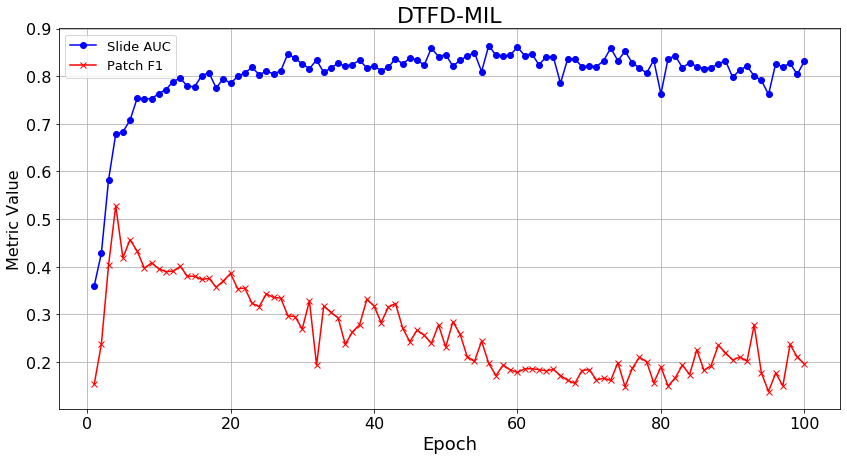
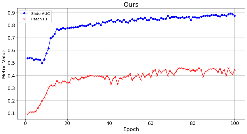
Figure 4: Comparision of slide and patch level classification performance on validation set during training

4.3 Results on Real-World Dataset

Table  1(a) shows the results of our method and other comparative methods on Camelyon16. For patch-level classification, FocusMIL and CausalMIL achieve significantly better results than the attention mechanism-based MIL. During the training process, we observed that the attention-based MIL approach achieved a high patch AUC at the beginning of training, but then gradually declined as the slide AUC increased, as shown in Figure 4. This suggests that the model learns to identify salient instances initially, but later relies on bag context information to fit to hard-to-classify slides. It is worth mentioning that DSMIL achieves better results compared to other attention-based methods. This improvement is attributed to DSMIL’s first stream using a max-pooling based instance-level classifier (Li, Li, and Eliceiri 2021); however, its second-stage attention network allows it to learn bag context information, which reduces its ability to recognize tumour concepts.

When the feature extractor is switched to CTransPatch, the patch-level classification performance of the attention-based MIL methods significantly improves but is still much worse than FocusMIL. This is because ResNet-18 is pre-trained on ImageNet and retains context patterns (Geirhos et al. 2018) in its features. In contrast, CTransPatch is pre-trained on WSI slides with self-supervised contrast learning, and its features help to reduce the dependency of attention-based models on bag context information.

For slide-level classification, FocusMIL significantly outperforms the former best-performing method, DTFD-MIL, in accuracy by $3.43\%$ with Resnet18 and $0.94\%$ with CTransPath, while slightly underperforming in AUC by $0.23\%$ and $0.08\%$, respectively.

Table 2: Performance Comparison on the TCGA Dataset.

Model	Slide AUC	Slide Acc
ABMIL	0.8900 (CI: 0.8654, 0.9146)	0.8200 (CI: 0.8036, 0.8364)
DSMIL	0.8909 (CI: 0.8849, 0.8970)	0.8295 (CI: 0.8154, 0.8436)
TransMIL	0.9501 (CI: 0.9456, 0.9547)	0.8886 (CI: 0.8778, 0.8993)
DTFD-MIL	0.9340 (CI: 0.9328, 0.9352)	0.8695 (CI: 0.8663, 0.8727)
IBMIL	0.9401 (CI: 0.9390, 0.9411)	0.8743 (CI: 0.8675, 0.8811)
CausalMIL	0.9298 (CI: 0.9256, 0.9339)	0.8791 (CI: 0.8654, 0.8927)
Ours	0.9360 (CI: 0.9309, 0.9411)	0.8819 (CI: 0.8742, 0.8896)

Table 2 presents the slide-level classification results on the TCGA-NSCLC dataset. The performance of FocusMIL is slightly below that of TransMIL but is comparable to DTFD-MIL, IBMIL, and CausalMIL. It is worth mentioning that the initial intention of proposing FocusMIL was to develop a reliable WSI classification method that performs well in tumour region localization and is unaffected by spurious correlations. These bag-based MIL models may exploit spurious correlations between bag context and labels to achieve better slide-level classification on some datasets, but the models will no longer be reliable when this correlation changes. Additionally, TransMIL does not provide a method for predicting patch labels.

Table 3: Performance on Camelyon16 Standard-MIL test dataset.

Model	Training	Testing
	Slide AUC	Slide AUC	Patch F1
ABMIL	1.000	0.007 (0.000, 0.021)	0.142 (0.117, 0.167)
DSMIL	1.000	0.377 (0.000, 0.776)	0.312 (0.165, 0.459)
TransMIL	1.000	0.001 (0.001, 0.002)	-
DTFD-MIL	1.000	0.010 (0.000, 0.034)	0.122 (0.080, 0.165)
IBMIL	1.000	0.000 (0.000, 0.001)	0.104 (0.098, 0.110)
CausalMIL	1.000	0.839 (0.823, 0.855)	0.373 (0.333, 0.412)
Ours	1.000	0.852 (0.835, 0.868)	0.402 (0.379, 0.425)

4.4 Results on Standard-MIL test

As shown in Table 3, all methods fit well in the training set. All of the tested attention-based methods have a test slide AUC less than 0.5, failing to respect the standard MIL assumption. CausalMIL and FocusMIL are little affected by the poison. Benefiting from the max-pooling based instance classifier, DSMIL performs well in patch-level classification, further demonstrating that max-pooling is crucial for learning positive concepts.

Table 4: Comparison of model size and training time per epoch of different MIL methods. The input dimension is set the same for each model to ensure fairness of comparison.

Model	Para.	Time	C16 ACC	TCGA ACC
ABMIL	657k	3.35s	0.8152	0.8200
DSMIL	856k	4.92s	0.7984	0.8295
TransMIL	2.66M	9.56s	0.8127	0.8886
DTFD-MIL	987k	6.02s	0.8032	0.8695
CausalMIL	302k	3.28s	0.8328	0.8791
Ours	167k	3.23s	0.8375	0.8819

4.5 Computational Cost Analysis

As shown in Table 4, FocusMIL has significantly fewer parameters compared to attention-based methods. Due to the use of mini-batch gradient descent with a batch size of 3, both CausalMIL and FocusMIL achieve superior training speeds. However, CausalMIL requires additional computations for reconstructing loss and the KL divergence loss of the conditional prior distribution, which results in slightly longer training times compared to FocusMIL. Although TransMIL shows better performance in the slide-level classification task on the TCGA-NLCSC dataset, its model size and training time are approximately 16 and 3 times greater than ours, respectively. Moreover, TransMIL could not provide patch-level predictions.

Table 5: Ablation study on Camelyon16 Dataset. Dropout was set at 0.4 for the second model.

Model	Mini-batch	Slide AUC	Patch F1
mi-Net		0.757 $\pm$ 0.122	0.298 $\pm$ 0.167
mi-Net+dropout		0.801 $\pm$ 0.027	0.384 $\pm$ 0.033
mi-Net+dropout	✓	0.635 $\pm$ 0.133	0.248 $\pm$ 0.118
FocusMIL(SGD)		0.814 $\pm$ 0.017	0.386 $\pm$ 0.022
FocusMIL	✓	0.860 $\pm$ 0.020	0.411 $\pm$ 0.035

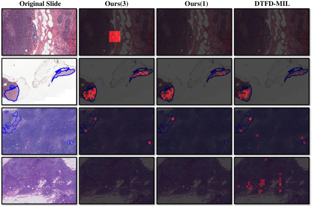
Figure 5: Visualization results of FocusMIL and DTFD-MIL on Camelyon16 dataset. Ours(3) and Ours(1) refer to the FocusMIL models trained with a batch size of 3 and 1, respectively. The fourth slide is negative. For FocusMIL, classifier confidence scores are utilized for patch intensities. For DTFD-MIL, patch probability derivation is used with a threshold of 0.5001.

4.6 Ablation Study

As shown in Table 5, the baseline model mi-Net is very unstable. In our experiments, we found that mi-Net may achieve high training slide-level AUC but extremely low patch-level AUCPR during training and fails completely during testing. This severe overfitting issue disappeared when the dropout was set above 0.4. However, this “training failure” reappeared when training mi-Net using mini-batch gradient descent, since establishing correct classification boundaries for salient and hard instances within a batch of multiple slides is more difficult. FocusMIL does not incorporate dropout; instead, forward amortized variational inference helps to avoid “training failure” and achieves a slide AUC that is 1.4% higher than mi-Net with a dropout of 0.4. Further significant improvements of 4.6% in slide AUC are obtained by training multiple bags together in a mini-batch. Since our method does not rely on bag-inherited information $\bm{Z}_{B}$ for classification, a higher slide AUC actually indicates better classification boundaries for hard instances, which is also confirmed by visualization results. For ablation study on TCGA-NSCLC dataset and experiments on the impact of batch size, please refer to the supplementary material.

4.7 Visualization

For fairness of comparison, the models for visualization are not deliberately selected, and both FocusMIL with a training batch size of 3 and DTFD-MIL models achieved a test slide AUC of approximately 0.87. As shown in Figure 5, our model accurately identifies both large and small tumour regions without any false positive predictions. FocusMIL with a training batch size of 1 misses some small tumour regions. For DTFD-MIL, it misses the tumour region in the first slide and some tumour patches in the second slide, and there are many false positive predictions. Notably, in the fourth slide, DTFD-MIL assigns high scores to many patches irrelevant to the tumour. After zooming in, the tissues in these regions are obviously blurrier, which is due to the slide preparation process. This confirms that DTFD-MIL can rely on bag-inherited information for predictions. We provide additional visualization results in the supplementary material.

5 Conclusion

This paper introduces FocusMIL, a method that respects the standard multiple instance learning assumption and incorporates variational inference to ensure the model focuses on tumour morphology. We further utilize mini-batch gradient descent to achieve better classification boundaries for identifying hard instances. Quantitative experiments demonstrate that our method significantly outperforms attention-based methods in patch-level classification and achieves competitive results at the slide-level compared to the current state-of-the-art. The visualization results demonstrate the superiority of our method in tumour region localization.

Broader Impact

The theoretical analysis presented in this paper indicates that attention-based methods cannot guarantee predictions based on the morphology of tumour cells (causal factor). Our quantitative experiments and visualizations also demonstrate that these methods fail to provide reliable tumour region predictions. To make matters worse, results from the Camelyon16 standard MIL test dataset show that attention-based methods can fail when there exists a strong spurious correlation between the bag context and the labels. Therefore, we emphasise that attention-based MIL methods should be used cautiously in WSI classification.

FocusMIL is a significantly more reliable alternative that focuses on causal factors for prediction. We recommend practitioners start with FocusMIL as a solid foundation to avoid excessive risk in deployment. Also, researchers can design more sophisticated WSI classification methods that satisfy the MIL hypothesis based on our FocusMIL.

Appendix A Additional Quantitative Experiments

A.1 Ablation Study on Hyperparameter

Ablation Study on Batch Size

Figure 6 shows the impact of different batch sizes on the model’s slide and patch level classification performance. Batch size greater than 1 can significantly improve the model’s slide-level classification performance. The improvement in patch F1-score is not pronounced. This is due to the fact that salient instances account for a rather high proportion of the overall positive instances, and the model’s ability to recognize hard instances will not be obviously reflected in an increase of the patch F1-score metric. A batch size that is too large can reduce the performance of the model, and we recommend choosing a batch size between 2 and 5.

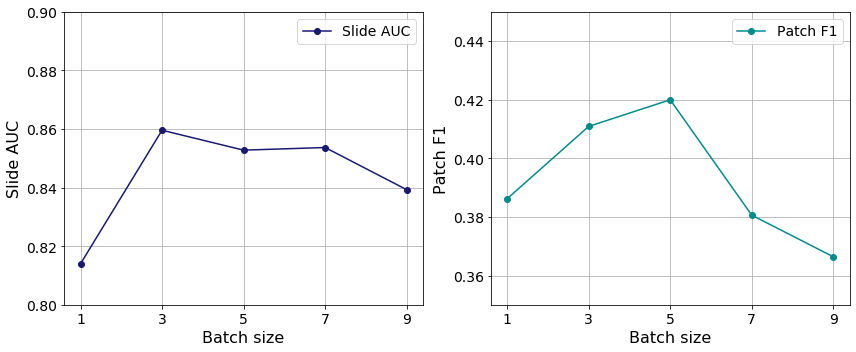
Figure 6: Results of ablation experiments on batch size.

Ablation Study on Dimentions of Latent Representation

As shown in Figure 7, our method is not sensitive to the parameter of latent dimension.

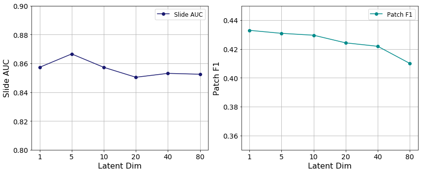
Figure 7: Results of ablation experiments on dimentions of latent representation

A.2 Ablation Study on TCGA-NSCLC Dataset

Since the positive instance ratio within the positive bags is high in this dataset, mi-Net did not encounter the “training failure” issues that occurred on the Camelyon16 dataset. With the introduction of forward amortized variational inference, FocusMIL improves 2.2% over mi-Net on the slide accuracy metric, and also improves 1.4% over mi-Net with dropout. Mini-batch gradient descent further improves FocusMIL’s performance by 1% on the slide accuracy metric. This improvement is smaller compared to the Camelyon16 dataset, possibly because the morphological differences in tumor cells are not as pronounced in the TCGA dataset as in the Camelyon16 dataset. Since the TCGA-NSCLC dataset does not have patch-level labels, this hypothesis is speculative. It is worth noting that mean-pooling outperforms max-pooling for aggregating slide-level predictions. However, we recommend that mean-pooling should be used with caution because mean-pooling does not respect the standard MIL assumption.

Table 6: Ablation study on TCGA-NSCLC dataset. Dropout was set at 0.4 for the second and third models. For the last two models, mean-pooling is used to aggregate patch-level predictions into slide-level predictions during test.

Model	Mini-batch	Slide AUC	Slide ACC
mi-Net		$0.904\pm 0.008$	$0.838\pm 0.023$
mi-Net+dropout		$0.913\pm 0.009$	$0.846\pm 0.015$
mi-Net+dropout	✓	$0.910\pm 0.009$	$0.850\pm 0.016$
FocusMIL		$0.916\pm 0.011$	$0.860\pm 0.016$
FocusMIL	✓	$0.919\pm 0.007$	$0.871\pm 0.005$
FocusMIL (mean)		$0.936\pm 0.004$	$0.882\pm 0.006$
FocusMIL (mean)	✓	$0.934\pm 0.005$	$0.879\pm 0.007$

Appendix B Additional Visualization

As shown in figure 8, DTFD-MIL generates false positive predictions for some patches of normal slides. After zooming in on these patches, we find that these patches that are given high positive probabilities are very blurry compared to the surrounding patches, likely due to bias introduced during the whole slide image production process. This confirms that attention-based methods may make predictions based on spurious correlations, leading to unreliable tumor localization. FocusMIL does not have any false-positive predictions for these normal slides

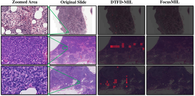
Figure 8: Visualization results of FocusMIL and DTFD-MIL on 3 normal slides. In the zoomed-in areas, some regions are relatively clear, while the rest are very blurred. DTFD-MIL may assign a high positive probability to the blurred regions.

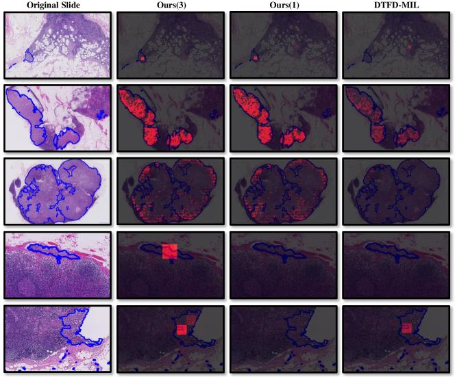
Figure 9: Additional visualization results of FocusMIL and DTFD-MIL on Camelyon16 dataset. Ours(3) and Ours(1) refer to the FocusMIL models trained with a batch size of 3 and 1, respectively. The tumour regions are delineated by the blue lines.

Figure 9 demonstrates the visualization results of FocusMIL and DTFD-MIL for five tumor slides. FocusMIL with a training batch size of 3 perfectly predicts all tumour regions. When the training batch size was changed to 1, FocusMIL misses some small tumour regions. This result confirms that training with mini-batch gradient descent does help to establish better classification boundaries for salient and hard instances. For DTFD-MIL, its predictions for both large and small tumour areas are suboptimal due to the fact that it can overfit on salient instances.

References

- Ambrogioni et al. (2019) Ambrogioni, L.; Güçlü, U.; Berezutskaya, J.; van den Borne, E.; Güçlütürk, Y.; Hinne, M.; Maris, E.; and van Gerven, M. 2019. Forward Amortized Inference for Likelihood-Free Variational Marginalization. In Chaudhuri, K.; and Sugiyama, M., eds., Proceedings of the Twenty-Second International Conference on Artificial Intelligence and Statistics, volume 89 of Proceedings of Machine Learning Research, 777–786. PMLR.
- Bejnordi et al. (2017) Bejnordi, B. E.; Veta, M.; Van Diest, P. J.; Van Ginneken, B.; Karssemeijer, N.; Litjens, G.; Van Der Laak, J. A.; Hermsen, M.; Manson, Q. F.; Balkenhol, M.; et al. 2017. Diagnostic assessment of deep learning algorithms for detection of lymph node metastases in women with breast cancer. Jama, 318(22): 2199–2210.
- Chen et al. (2021) Chen, R. J.; Lu, M. Y.; Shaban, M.; Chen, C.; Chen, T. Y.; Williamson, D. F.; and Mahmood, F. 2021. Whole Slide Images are 2D Point Clouds: Context-Aware Survival Prediction Using Patch-Based Graph Convolutional Networks. In International Conference on Medical Image Computing and Computer-Assisted Intervention, 339–349.
- Deng et al. (2009) Deng, J.; Dong, W.; Socher, R.; Li, L.-J.; Li, K.; and Fei-Fei, L. 2009. Imagenet: A large-scale hierarchical image database. In 2009 IEEE conference on computer vision and pattern recognition, 248–255. Ieee.
- Dietterich, Lathrop, and Lozano-Pérez (1997) Dietterich, T. G.; Lathrop, R. H.; and Lozano-Pérez, T. 1997. Solving the multiple instance problem with axis-parallel rectangles. Artificial intelligence, 89(1-2): 31–71.
- Foulds and Frank (2010) Foulds, J.; and Frank, E. 2010. A review of multi-instance learning assumptions. The knowledge engineering review, 25(1): 1–25.
- Geirhos et al. (2018) Geirhos, R.; Rubisch, P.; Michaelis, C.; Bethge, M.; Wichmann, F. A.; and Brendel, W. 2018. ImageNet-trained CNNs are biased towards texture; increasing shape bias improves accuracy and robustness. In International Conference on Learning Representations.
- He et al. (2016) He, K.; Zhang, X.; Ren, S.; and Sun, J. 2016. Deep residual learning for image recognition. In Proceedings of the IEEE conference on computer vision and pattern recognition, 770–778.
- Ilse, Tomczak, and Welling (2018) Ilse, M.; Tomczak, J.; and Welling, M. 2018. Attention-based deep multiple instance learning. In International conference on machine learning, 2127–2136. PMLR.
- Jögi et al. (2012) Jögi, A.; Vaapil, M.; Johansson, M.; and Påhlman, S. 2012. Cancer cell differentiation heterogeneity and aggressive behavior in solid tumors. Upsala journal of medical sciences, 117(2): 217–224.
- Keum et al. (2024) Keum, S.; Kim, S.; Lee, S.; and Lee, J. 2024. Revisiting Subsampling and Mixup for WSI Classification: A Slot-Attention-Based Approach.
- Kingma and Welling (2013) Kingma, D. P.; and Welling, M. 2013. Auto-encoding variational bayes. arXiv preprint arXiv:1312.6114.
- Li, Li, and Eliceiri (2021) Li, B.; Li, Y.; and Eliceiri, K. W. 2021. Dual-stream Multiple Instance Learning Network for Whole Slide Image Classification with Self-supervised Contrastive Learning. In 2021 IEEE/CVF Conference on Computer Vision and Pattern Recognition (CVPR), 14313–14323.
- Lin et al. (2023) Lin, T.; Yu, Z.; Hu, H.; Xu, Y.; and Chen, C.-W. 2023. Interventional bag multi-instance learning on whole-slide pathological images. In Proceedings of the IEEE/CVF Conference on Computer Vision and Pattern Recognition, 19830–19839.
- Lu et al. (2021) Lu, M. Y.; Williamson, D. F.; Chen, T. Y.; Chen, R. J.; Barbieri, M.; and Mahmood, F. 2021. Data-efficient and weakly supervised computational pathology on whole-slide images. Nature Biomedical Engineering, 5(6): 555–570.
- Qu et al. (2024) Qu, L.; Ma, Y.; Luo, X.; Guo, Q.; Wang, M.; and Song, Z. 2024. Rethinking multiple instance learning for whole slide image classification: A good instance classifier is all you need. IEEE Transactions on Circuits and Systems for Video Technology.
- Qu et al. (2022) Qu, L.; Wang, M.; Song, Z.; et al. 2022. Bi-directional weakly supervised knowledge distillation for whole slide image classification. Advances in Neural Information Processing Systems, 35: 15368–15381.
- Raff and Holt (2023) Raff, E.; and Holt, J. 2023. Reproducibility in Multiple Instance Learning: A Case For Algorithmic Unit Tests. In Thirty-seventh Conference on Neural Information Processing Systems.
- Shao et al. (2021) Shao, Z.; Bian, H.; Chen, Y.; Wang, Y.; Zhang, J.; Ji, X.; et al. 2021. TransMIL: Transformer based Correlated Multiple Instance Learning for Whole Slide Image Classification. Advances in Neural Information Processing Systems, 34: 2136–2147.
- Tang et al. (2023) Tang, W.; Huang, S.; Zhang, X.; Zhou, F.; Zhang, Y.; and Liu, B. 2023. Multiple instance learning framework with masked hard instance mining for whole slide image classification. In Proceedings of the IEEE/CVF International Conference on Computer Vision, 4078–4087.
- Tang et al. (2024) Tang, W.; Zhou, F.; Huang, S.; Zhu, X.; Zhang, Y.; and Liu, B. 2024. Feature Re-Embedding: Towards Foundation Model-Level Performance in Computational Pathology. In Proceedings of the IEEE/CVF Conference on Computer Vision and Pattern Recognition, 11343–11352.
- Vaswani et al. (2017) Vaswani, A.; Shazeer, N.; Parmar, N.; Uszkoreit, J.; Jones, L.; Gomez, A. N.; Kaiser, Ł.; and Polosukhin, I. 2017. Attention is all you need. Advances in neural information processing systems, 30.
- Wang et al. (2018) Wang, X.; Yan, Y.; Tang, P.; Bai, X.; and Liu, W. 2018. Revisiting multiple instance neural networks. Pattern Recognition, 74(C): 15–24.
- Wang et al. (2022) Wang, X.; Yang, S.; Zhang, J.; Wang, M.; Zhang, J.; Yang, W.; Huang, J.; and Han, X. 2022. Transformer-based unsupervised contrastive learning for histopathological image classification. Medical image analysis, 81: 102559.
- Yao et al. (2020) Yao, J.; Zhu, X.; Jonnagaddala, J.; Hawkins, N.; and Huang, J. 2020. Whole Slide Images based Cancer Survival Prediction using Attention Guided Deep Multiple Instance Learning Networks. Medical Image Analysis, 65: 101789.
- Zhang et al. (2022a) Zhang, H.; Meng, Y.; Zhao, Y.; Qiao, Y.; Yang, X.; Coupland, S. E.; and Zheng, Y. 2022a. DTFD-MIL: Double-tier feature distillation multiple instance learning for histopathology whole slide image classification. In Proceedings of the IEEE/CVF Conference on Computer Vision and Pattern Recognition, 18802–18812.
- Zhang et al. (2022b) Zhang, W.; Zhang, X.; Zhang, M.-L.; et al. 2022b. Multi-instance causal representation learning for instance label prediction and out-of-distribution generalization. Advances in Neural Information Processing Systems, 35: 34940–34953.
- Zhang et al. (2023) Zhang, Y.; Li, H.; Sun, Y.; Zheng, S.; Zhu, C.; and Yang, L. 2023. Attention-challenging multiple instance learning for whole slide image classification. arXiv preprint arXiv:2311.07125.
- Zhang et al. (2022c) Zhang, Y.; Sun, Y.; Li, H.; Zheng, S.; Zhu, C.; and Yang, L. 2022c. Benchmarking the robustness of deep neural networks to common corruptions in digital pathology. In International Conference on Medical Image Computing and Computer-Assisted Intervention, 242–252. Springer.
- Zhou and Zhang (2002) Zhou, Z.-H.; and Zhang, M.-L. 2002. Neural networks for multi-instance learning. In Proceedings of the International Conference on Intelligent Information Technology, Beijing, China, 455–459. Citeseer.