Laser cooling a 1-milligram torsional pendulum to 240 microkelvins

Abstract

Milligram-scale mechanical oscillators hold potential for testing fundamental physical phenomena on various fronts, including laboratory-scale effects at the interface of quantum mechanics and gravity. Nevertheless, experimental realizations supporting this potential have thus far been lacking. Here, we present a new level of control over a 1-milligram torsional pendulum, demonstrating laser feedback cooling of its torsional motion from room temperature to 240 microkelvins, establishing the coldest mechanical motion in the microgram-to-kilogram mass window – a factor of 25 beyond prior art. The developed system shows a unique torque sensing capability, reaching $1.2\times 10^{-18}$ N$\cdot$m/$\sqrt{\textrm{Hz}}$ thermal-noise-limited sensitivity – a factor of 10 below the state of the art for the milligram scale. With readily feasible improvements in the pendulum suspension, a further 100-fold reduction in both achievable temperatures and torque sensitivities is foreseen, pushing towards operation in the quantum regime at such large mass scales.

There has been growing enthusiasm surrounding the development of micro-to-milligram-scale oscillators for precision tests of physics Westphal et al. (2021); Fuchs et al. (2024); Cataño Lopez et al. (2020); Matsumoto et al. (2019); Hofer et al. (2023); Kawasaki et al. (2022); Komori et al. (2020); Raut et al. (2021); Agatsuma et al. (2014). While explorations of gram-to-ton-scale oscillators opened up the possibility of observing gravitational wave phenomena Abbott et al. (2016), and femto-to-microgram-scale oscillators the door to quantum mechanics with solid-state mechanical objects Aspelmeyer et al. (2014a), the mesoscopic nature of the micro-to-milligram scale offers new possibilities – notably, the simultaneous exploration of quantum mechanics and gravity. Oscillators in this mass scale appear in proposals Krisnanda et al. (2020); Miao et al. (2020); Miki et al. (2024) for experimental studies of gravity-mediated entanglement Bose et al. (2017); Marletto and Vedral (2017), optomechanical entanglement Vitali et al. (2007); Müller-Ebhardt et al. (2008), quantum decoherence Bose et al. (1999); Marshall et al. (2003), semi-classical gravity Gan et al. (2016), and spontaneous wave function collapse Diósi (2015). Furthermore, the milligram scale provides a unique parameter space not covered by other potential experiments for dark matter searches Carney et al. (2021), and for experiments searching for deviations from Newtonian gravity Qvarfort et al. (2022).

Although glimpses of quantum noise have already been observed even in the motion of the 10-kg-scale LIGO mirrors utilizing megawatts of circulating light Yu et al. (2020), conventional optomechanical methods favor much smaller masses for quantum mechanics to be relevant Aspelmeyer et al. (2014a). The milligram domain presents a compromise, with masses large enough for gravity to be important Westphal et al. (2021); Raut et al. (2021), yet sufficiently small to potentially make quantum effects in motion dominant Michimura and Komori (2020). Given the low oscillation frequencies (100 mHz to 100Hz), experiments in this domain are very sensitive to vibrations Komori et al. (2020); Whittle et al. (2021). At this mass scale, a good option for environmental isolation of the masses is to suspend them with thin fibers to form pendulums (see also magnetic levitation efforts Raut et al. (2021); Fuchs et al. (2024)). Our interest in torsional (instead of swing) motion arises due to its efficient decoupling from ground movements, which makes it a natural choice for precision sensing applications. We note a growing body of recent work pursuing quantum optics experiments with angular motion Pratt et al. (2023); Hao and Purdy (2024); Tebbenjohanns et al. (2023); Su et al. (2023); Komori et al. (2020); Hu et al. (2023).

For an optomechanical system, a prerequisite for observing quantum effects in motion is the domination of quantum radiation pressure noise (QRPN) over all other noise sources Michimura and Komori (2020). This regime has been reached for a number of physical systems with sub-microgram masses Aspelmeyer et al. (2014b); Delić et al. (2020); Underwood et al. (2015); Cripe et al. (2019); Rossi et al. (2018); Clark et al. (2017); Wilson et al. (2015), but no mechanical oscillator heavier than tens of micrograms has been brought into the QRPN-limited regime or to the quantum ground state of motion for that matter Whittle et al. (2021). Due to the low natural oscillation frequencies of the pendulums considered here, QRPN domination typically implies the possibility of cooling to the motional ground state Michimura and Komori (2020), given demonstrated abilities to significantly shift oscillation frequencies without introducing excess noise by optically or electronically trapping the pendulums. This can vastly increase not only the oscillation frequency, but also the apparent quality factors $Q_{app}$. This dissipation dilution effect has been demonstrated in passive systems featuring optical cavities Komori et al. (2020); Corbitt et al. (2007); Matsumoto et al. (2016), standing waves Ni et al. (2012), or engineered mechanical stresses Pratt et al. (2023); and alternatively, it has been achieved with active feedback systems Whittle et al. (2021). The frequency shifting strategy is expected to be particularly effective for suspended pendulums, since the ultimate mechanism that sets loss levels – structural damping – exhibits a peculiar behavior, where loss is reduced at frequencies above the natural resonance, allowing increased levels of dissipation dilution Komori et al. (2022).

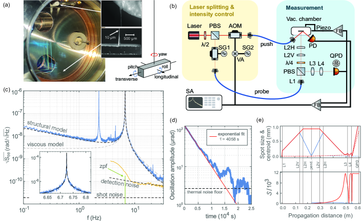
Figure 1: Experimental setup and its characterization. (a) Photo of the pendulum inside the vacuum chamber. Insets: Tapered suspension fiber ends and the pendulum mirror bar. Overlay: Pendulum mode definitions. (b) Schematics of the optical setup. PBS: polarizing beam splitter, $\lambda/2$: half-wave plate, $\lambda/4$: quarter-wave plate, AOM: acousto-optic modulator, SG: signal generator, VA: variable attenuator, SA: digitization and spectrum analysis, FB: feedback circuit, PD: photodetector, QPD: quadrant photodetector, L2H(V): horizontal (vertical) cylindrical lens with 200 mm (60 mm) focal length, L1(3, 4): spherical lens with 4.5 mm (10 mm, 4.0 mm) focal length. (c) Steady-state yaw noise spectrum (blue) compared to thermal noise models (dashed lines) with structural or viscous damping. Inset: close-up of the resonance peak, orange data: detection noise spectrum compared to theoretical laser shot-noise Pratt et al. (2023), “zpf” line: peak level of the spectrum for quantum zero-point fluctuations associated with the yaw motion for reference. The parasitic 2.27-Hz peak is due to the residual swing motion sensitivity in the yaw channel. The “detection noise” model incorporates a variable “white + 1/f” noise to fit the data above 8 Hz. (d) Ring-down measurement of the 6.72-Hz yaw oscillations. (e) Implemented probe beam profile across the lens system for horizontal (red) and vertical (blue) directions. Top; solid lines: beam spot size evolution, dashed lines: beam centroid evolution for a 100-$\mu\text{rad}$ illustrative yaw (red) or pitch (blue) rotation of the pendulum. Bottom; evolution of the tilt sensitivity parameter $\mathcal{S}$.

The level of control over a mechanical oscillator can be effectively assessed by the amount of cooling demonstrable in the system, providing a point of comparison to a wide range of physical systems. In this work, we achieve laser cooling of the torsional motion of a 1-milligram suspended mirror from room temperature to an effective temperature of $240~{}\mu\text{K}$ without the use of an optical cavity. This result significantly surpasses the lowest reported motional temperatures in the microgram-to-kilogram mass window, which were 6 mK for the gram scale Corbitt et al. (2007) and 15 mK for the milligram scale Matsumoto et al. (2016) – both realized in optical cavity systems. The motion of the pendulum is detected using an optimized optical lever, and radiation pressure forces are used for its control. The cooling is achieved by first optically trapping the torsional motion to increase its frequency from 6.72 Hz to 18.0 Hz, and then by critically damping the motion. This level of manipulation is possible only after taking under control many other oscillatory modes of the pendulum. In addition to the achieved motion control, we directly observe a torque sensitivity of $1.2\times 10^{-18}$N$\cdot$m/$\sqrt{\textrm{Hz}}$, constituting a record value for the milligram scale – a factor of 10 beyond Ref. Komori et al. (2020). This thermal-noise-limited sensitivity allows for a very clear demonstration of the peculiar properties of structural damping for nearly three decades of a frequency range in our setup.

Setup
The pendulum used in this study is shown in Fig. 1(a) inside its vacuum housing maintained at 5$\crossproduct$10^-9-mbar by an ion pump. The pendulum consists of a $2\times 0.5\times 0.5$ mm³ silver-coated fused silica mirror bar, and a 10-$\mu\text{m}$ diameter fused silica suspension fiber of 5-cm length. It exhibits a torsional (yaw) resonance at $f_{0}\equiv\omega_{0}/2\pi=6.72$ Hz in addition to longitudinal and transverse swing modes at 2.27 Hz, a roll mode at 44.48 Hz, and a pitch mode at 125.95 Hz (Fig. 1(a), overlay). The pendulum bar piece was cut from a larger optical mirror, and the suspension fiber was manufactured in-house from a standard 125-µm-diameter optical fiber (S630-HP) by wet etching. The etching process was designed to leave 500 µm long tapers at both ends (Fig. 1(a), inset) to allow adhiesive-aided attachment without introducing mechanical losses. In this way, the torsional energy is mainly stored in the high-compliance thin section of the fiber, preventing dissipation at the low-compliance 125-µm diameter adhesive-bonded (Norland 61) surfaces. This design achieves a quality factor of $Q_{0}=\tau\omega_{0}/2=8.6\times 10^{4}$ for the yaw mode, as measured by a ring-down of its oscillation amplitude with a time constant of $\tau=4058$ s (Fig. 1(d)). The motion thermally equilibrates around $(k_{B}T/(I\omega_{0}^{2}))^{1/2}=2.5~{}\mu\text{rad}$ fluctuations dictated by the equipartition theorem – here, moment of inertia $I=3.7\times 10^{-13}~{}\text{kg}\cdot\text{m}^{2}$, temperature $T=300~{}\text{K}$, Boltzmann’s constant $k_{B}$. The measured $Q_{0}$ and the corresponding mechanical energy dissipation rate of $\gamma_{0}=\omega_{0}/Q_{0}=2\pi\times 79~{}\mu\text{Hz}$ indicate excellent performance even compared to monolithic pendulums manufactured with laser-welded suspensions Cataño Lopez et al. (2020) – with room only for a factor of 2-3 improvement given standard material loss limitations for the utilized fiber’s surface-to-volume ratio Gretarsson and Harry (1999).

The near-ideal thermally-limited noise spectrum (Fig. 1(c)) reveals that dissipation in the yaw motion arises purely from structural damping, with no observable viscous contribution from background gas. This spectrum arises from a thermal (th) torque ($\tau$) noise of power spectral density (PSD) $S_{\tau\tau}^{th}=4k_{B}TI\gamma(\omega)$ with frequency-dependent structural dissipation rate $\gamma(\omega)=\gamma_{0}\frac{\omega_{0}}{\omega}$ Michimura and Komori (2020). The torque noise manifests itself as an angular ($\theta$) PSD $S_{\theta\theta}^{th}=|\chi|^{2}S_{\tau\tau}^{th}$ through the mechanical susceptibility $\chi(\omega)=(\omega_{0}^{2}-w^{2}+i\omega\gamma(\omega))^{-1}/I$, showing excellent agreement with the measurements. The agreement in the peak region (Fig. 1(c), inset) indicates a resonance frequency instability below $100~{}\mu\text{Hz}$.

The characterization of the motion is enabled by an optical lever capable of resolving the motion at the level of quantum zero-point fluctuations (zpf) $S_{\theta\theta}^{zpf}=S_{\theta\theta}^{th}/(2n_{th})$ that would be associated with the yaw oscillations (Fig. 1(c)). Here, $n_{th}=9.3\times 10^{11}$ is the mean number of thermal excitation quanta at 300 K. The optical lever signal calibration was done by replacing the pendulum with a rigid rotatable mirror. Based on this calibration, the measured yaw angle noise agrees with the expected thermal noise levels to within 10%. The detection noise spectrum shown in Fig. 1(c) is the base noise of the optical lever obtained in this rigid mirror configuration.

The optical setup around the pendulum is shown in Figure 1(b). The output of a 780-nm DFB laser is split into two paths: one to probe the pendulum’s motion (10 $\mu$W) and the other to manipulate it through radiation pressure (0-4 mW). Accousto-optic modulators (AOM) enable intensity control on each path. The Gaussian probe beam is incident at the center of the pendulum, and circulates back to a quadrant photodiode (QPD), which reads the horizontal and vertical positions of the beam to yield the pendulum motion.

An arrangement of cylindrical and spherical lenses maximizes the sensitivity to yaw motion (horizontal beam tilt), while minimizing the sensitivity to any type of mechanical mode that leads to a pitching motion component (vertical beam tilt). The beam shaping principle is based on two considerations: 1) independently of beam divergence, the fundamental tilt sensitivity is linearly proportional to the beam spot size $\text{w}_{p}$ at the pendulum, and 2) the tilt sensitivity parameter $\mathcal{S}=\sqrt{\frac{8}{\pi}}\frac{d}{d\theta}\frac{\delta(\theta)}{\text{w}}~{}~{}(\text{rad}^{-1})$ that we utilize can be maximized to $\mathcal{S}_{\text{max}}=\tfrac{\sqrt{32\pi}}{\lambda}\text{w}_{p}$ for any desired beam size at the detection point, extracting the tilt information optimally (see Methods). In the definition of the sensitivity parameter, w and $\delta(\theta)$ are the spot size and the tilt-induced beam displacement at the detection point; and $\lambda$ is the wavelength. With these definitions, the quantity $1/(\mathcal{S}~{}\theta)^{2}$ has the interpretation of the total number of photons required for the QPD to resolve a pendulum tilt $\theta$. The implemented probe beam profile and the sensitivity $\mathcal{S}$ as a function of detection distance are illustrated in Fig. 1(e). $\mathcal{S}$ is maximized in the horizontal channel and minimized in the vertical one, both for a large spot size at the detection point, avoiding photodiode gaps.

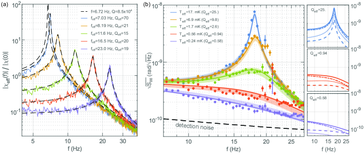
Figure 2: Feedback control of the motion. (a) Experimental effective susceptibilities as the resonance frequency of the pendulum is shifted under feedback control. Normalization is to the DC value of the feedback-free susceptibility. (b) Noise spectral densities for different feedback damping strengths for a pendulum shifted to 18 Hz. Data points: mean spectral density within each 2.4-Hz frequency bin, error bars: $\pm 1$ standard deviation within each bin, solid lines: theoretical noise models with excess vibration noise as a fit parameter, error bands: uncertainty in model fits due to varying lab vibration noise levels, detection noise: same as Fig. 1. Side panels show the noise breakdown for the resulting theory models for chosen damping strengths. Solid lines: total noise, dash-dotted lines: theoretical thermal noise given the effective susceptibilities, dashed lines: theoretical imprinted measurement noise, dotted lines: extracted white-torque-noise equivalent vibration noise.

The QPD output is fed into a home-built analog feedback circuit to control the push beam power incident on the corner of the pendulum to implement effective equations of motion for the yaw mode (Fig. 1(b)). Although the detection is optimized for the yaw motion, smaller signals from all other modes of the pendulum are also available on the QPD output. We use these to dampen the other modes via feedback by pushing on the vacuum chamber with piezo-actuators (see Methods).

Results
The feedback-based radiation forces are designed to implement the effective susceptibility function

$$\chi_{\text{eff}}(\omega)=(\omega_{\text{eff}}^{2}-w^{2}+i\omega\gamma_{\text{eff}})^{-1}/I$$ (1)

of a torsional harmonic oscillator with tunable frequency and damping. The analog feedback circuit implementing the effective susceptibility contains two key parameters: gain of the feedback loop $g$ and the lead-filter corner frequency $\omega_{\text{lead}}$. Physically, while the gain controls the strength of the applied restoring torque, the lead filter introduces the time derivative of the measured yaw angle, implementing velocity damping (see Methods). The two parameters dictate the effective resonance frequency $\omega_{\text{eff}}=\omega_{0}\sqrt{1+g}$ and the effective damping rate $\gamma_{\text{eff}}=\frac{\omega_{0}^{2}g}{\omega_{\text{lead}}}+\gamma(\omega)$. Here, the intrinsic damping $\gamma(\omega)$ is negligible relative to the feedback damping term, rendering the effective damping independent of frequency (purely viscous) with an effective quality factor of $Q_{\text{eff}}=\frac{\omega_{\text{eff}}}{\gamma_{\text{eff}}}$.

Fig. 2(a) illustrates our ability to shift the torsional oscillation frequency through feedback-based optical forces, realizing an optical torsion spring. To experimentally characterize the effective susceptibilities, we optically apply a white-noise torque drive to the pendulum that is about 100 times the thermal torque noise. This creates a large motion, enabling an easy measurement of the angular noise spectrum to calculate $|\chi_{\text{eff}}|=(S_{\theta\theta}/S_{\tau\tau})^{1/2}$. During these measurements, we additionally induce a level of feedback-damping to stay below the maximal restoring torque that can be supplied by the finite power of the push beam. For each configuration, the effective frequencies and quality factors are extracted by fitting Eq. 1 to the data, obtaining excellent agreement with the intended effective susceptibilities.

Unlike the restoring torsion provided by the suspension fiber, which brings in thermal torque noise, the optically induced torques can practically be noise-free Komori et al. (2022). An oscillator whose frequency is increased by an optical spring acquires a new set of apparent parameters that dictate its properties. Defining the apparent quantities for the case of ‘no induced feedback damping’, the susceptibility describing the oscillator becomes $\chi_{\text{app}}(\omega)=(\omega_{\text{eff}}^{2}-w^{2}+i\omega\gamma(\omega))^{-1}/I$, where $\gamma(\omega)$ is the original structural damping function. The resonant damping rate decreases to $\gamma_{\text{app}}=\gamma(\omega_{\text{eff}})=\gamma_{0}\frac{\omega_{0}}{\omega_{\text{eff}}}$, and the resonant quality factor increases to

$$Q_{\text{app}}=\frac{\omega_{\text{eff}}}{\gamma_{\text{app}}}=Q_{0}\left(\frac{\omega_{\text{eff}}}{\omega_{0}}\right)^{2}.$$ (2)

The larger the apparent quality factor, the more one can cool the oscillator. To understand this, note that feedback cooling sets the value of $\gamma_{\text{eff}}$ in Eq. 1, reducing the resonance peak height without adding noise. The largest meaningful value of $\gamma_{\text{eff}}$ is achieved at critical damping $Q_{\text{eff}}=1/2$, after which point there is no oscillator. Therefore one needs to start with a high quality factor to be able to achieve large cooling factors.

To explore the limits of our ability to cool the yaw motion, we shift the yaw-mode resonance to 18 Hz, to the center of the excess-noise-free frequency band from 8 to 28 Hz. Below 8 Hz, spurious detection noise kicks in; above 28 Hz, excess noise of the 44-Hz roll motion leaks into the yaw-angle measurement. For the 18-Hz oscillator, the apparent quality factor is $Q_{app}=6.1\times 10^{5}$. After shifting the frequency, we implement five different feedback circuit configurations with effective damping rates corresponding to quality factors ranging from $Q_{\text{eff}}=25$ to $Q_{\text{eff}}=0.58$. We characterize the resulting effective susceptibilities using the same procedure described in the context of Fig. 2(a). Then, for each feedback configuration, we let the system operate without any external driving torque. Fig. 2(b) shows the yaw motion noise spectra obtained, showing the progressively colder oscillator sates.

The resulting motion is governed by conversion of three torque noise contributions to angular motion: structural thermal noise, detection noise that is imprinted on the motion through the feedback loop, and vibrations that affect the yaw motion (see Methods for model details). Given the theoretical thermal noise, the characterized susceptibilities, and the detection noise, the only unknown is the vibrations in the system, which are known to vary over time. We take the vibration spectra to be approximately white noise (in torque) within the frequency band of interest and set its amplitude to be the fit parameter for the overall model. The resulting model curves are shown together with the spectral noise data in Fig. 2(b). The noise breakdown is illustrated in the right panel Fig. 2(b) as well for exemplary cases: the system is always driven dominantly by thermal noise, and the measurement noise imprinted by the system and the vibration noise are always subdominant.

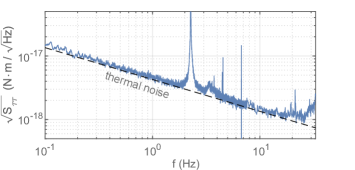
Figure 3: Free running torque-referred angular noise $S_{\tau\tau}\equiv S_{\theta\theta}/|\chi|^{2}$, characterizing the torque sensitivity. The loss of sensitivity around 2.2 Hz is due to leakage of the pendulum swing mode signals into the yaw channel.

The extent of the fluctuations in the yaw angle $\theta$ around zero serves as an indicator of the average energy in the torsional mode, allowing the assignment of an effective temperature $T_{\text{eff}}=I\omega_{\text{eff}}^{2}\expectationvalue{\theta^{2}}/k_{B}$ to this motion. In this context, the yaw angle fluctuations are determined by the integral of the angular PSD: $\expectationvalue{\theta^{2}}=\int_{0}^{\infty}S_{\theta\theta}(f)df$. The value of this integral is dominated by the contributions within the vicinity of the resonance peak. In fact, under the action of thermal noise alone, taking the PSD for the case of a purely frequency-shifted pendulum $S_{\theta\theta}^{\text{app}}=|\chi_{\text{app}}|^{2}S_{\tau\tau}^{th}$, one recovers to a good approximation the equipartition theorem $I\omega_{\text{eff}}^{2}\expectationvalue{\theta^{2}}_{\text{app}}\!\!=k_{B}T$ Komori et al. (2022); Whittle et al. (2021) – already reaching to a 94% accuracy even within a small integration band of $10\frac{\gamma_{\text{app}}}{2\pi}\equiv 0.29~{}\text{mHz}$. Experimentally, the achieved effective temperatures can be determined by referencing the observed angular fluctuations within the accessible observation band to those of the ideal frequency-shifted oscillator:

$$\frac{T_{\text{eff}}}{T}=\frac{\int_{f_{1}}^{f_{2}}S_{\theta\theta}(f)~{}df}{\int_{f_{1}}^{f_{2}}S_{\theta\theta}^{\text{app}}\!(f)~{}df}.$$ (3)

In our case, $f_{1}=8~{}\text{Hz}$ and $f_{2}=28~{}\text{Hz}$. For each damping configuration in Fig. 2(b), the temperatures extracted using Eq. 3 are indicated, reaching down to a minimum of to 240 $\mu\text{K}$ near critical damping. This temperature corresponds to a mean phonon occupation number of $n=2.8\times 10^{5}$.

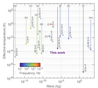
Figure 4: Comparison to achieved mechanical mode cooling in other physical systems. Arrows run from starting temperatures to final reached temperatures, with the remaining mode excitation quanta additionally indicated. Tip-only arrows indicate experiments based solely on refrigeration. Colors encode oscillation mode frequencies, illustrating ground-state cooling requires lower temperatures for lower frequency oscillators. Experiments: (a) nanobead Delić et al. (2020), (b) nanobeam Wilson et al. (2015), (c) membrane Schmid et al. (2022), (d) membrane Rossi et al. (2018), (e) torsional nanofiber Tebbenjohanns et al. (2023), (f) cantilever Zoepfl et al. (2023), (g) membrane Underwood et al. (2015), (h) superconducting microbead Hofer et al. (2023), (i) acoustic resonator Bild et al. (2023), (j) pendulum Matsumoto et al. (2016), (k) pendulum Corbitt et al. (2007), (l) LIGO pendulums Whittle et al. (2021), (m) bar resonator Vinante et al. (2008).

In addition to the demonstrated optomechanical control capabilities, the developed pendulum system is very competitive as a sensor. The torque sensitivity is primarily limited by structural thermal noise, and reaches a minimal observed value of $1.2\times 10^{-18}$ around 20 Hz. This corresponds to a broadband angular acceleration sensitivity of $3.3\times 10^{-6}~{}\text{rad}\cdot\text{s}^{-2}/\sqrt{\text{Hz}}$, or, when referred to the tip of the pendulum, to a broadband linear acceleration sensitivity of $3.3\times 10^{-10}\text{g}/\sqrt{\text{Hz}}$. This value is on par with state-of-the-art resonant acceleration sensitivities achievable with magnetically levitated particles at the 1-milligram level in cryogenic systems Fuchs et al. (2024).

Outlook
The presented work sets a benchmark of performance by demonstrating the lowest achieved effective temperatures for a mechanical mode of an object in the mass range from 100 ng to 1 kg (see Fig. 4), and the lowest reported torque noise in the milligram scale Komori et al. (2020). The level of control achieved highlights feasibility of operating milligram-scale oscillators in the quantum regime in the near future, pointing to an avenue for exploration of the interface of quantum mechanics and gravity at a mass scale where domination of gravitational interactions can be achieved relatively easily Westphal et al. (2021). To understand the capabilities achievable with the demonstrated optical torsional spring, we note that for a 1-$\mu\text{m}$-diameter suspension fiber (e.g., Cataño Lopez et al. (2020)), a 65 mHz torsional oscillator will be realized in the current configuration. Frequency shifting to 18 Hz, for example, will result in an apparent quality factor in the $10^{9}$ scale. Taking into account all sources of noise that exist in the current setup, a further 100-fold improvement in both achievable temperatures and torque sensitivities can be obtained. Cooling beyond that level, towards the quantum ground state, would make the use of optical cavities engineered for torsional motion Agafonova et al. (2024) desirable. Even without additional improvements, readily achieved torque noises imply technologically relevant acceleration sensitivities for testing models of modified Newtonian dynamics (MOND) using additional small gravitational source masses Timberlake et al. (2021).

 

Methods

.1 Optimal tilt sensing with a split photodiode

Here, we derive the optimal sensitivity achievable for tilt sensing using a split photodiode, and introduce the tilt sensitivity parameter utilized in the main text.

After reflection of a Gaussian beam incident on a pendulum tilted by an angle $\theta$, the beam will acquire a $2\theta$ tilt with respect to an untilted reference axis. A beam tilt by angle $2\theta$ is equivalent to introducing a position-dependent phase shift $2\theta k_{0}x$ on the beam, where $x$ is the coordinate perpendicular to the propagation axis and $k_{0}=2\pi/\lambda$ is the wave number in terms of the wavelength $\lambda$. For small angles, the phase factor can be expressed as $e^{i2\theta k_{0}x}\approx 1+i2\theta k_{0}x$, and the reflected beam profile can be described as a sum of zeroth-order and first-order Hermit-Gauss modes, as we will illustrate. In the following, we will make use of the normalized Hermite-Gauss mode functions

$$\begin{split}&\phi_{0}(x,z)=\tfrac{2^{1/4}}{(\pi\text{w}^{2}(z))^{1/4}}e^{-x^{2}/\text{w}^{2}(z)}e^{-ik_{0}x^{2}/2R(z)}e^{i\varphi(z)}\\ &\phi_{1}(x,z)=\phi_{0}(x,z)\tfrac{2x}{\text{w}(z)}e^{i\varphi(z)}.\end{split}$$ (S1)

Here, $z$ is the propagation distance along the reference axis, and $\text{w}(z)$, $R(z)$ and $\varphi(z)$ are the propagation-distance-dependent spot size, wavefront curvature, and Gouy phase, respectively. The Gouy phase covers a range of $\pi$ radians as $z$ goes from $-\infty$ to $\infty$.

We will take the pendulum to be located at $z_{p}$. Right after the pendulum, the incident beam represented by the wave $\psi(x,z_{p})=\phi_{0}(x,z_{p})$ at the location of the pendulum will evolve into

$$\begin{split}\psi^{\prime}(x,z_{p})&=\phi_{0}(x,z_{p})e^{ik_{0}2\theta x}\\ &\approx\phi_{0}(x,z_{p})+ie^{-i\varphi(z_{p})}\theta k_{0}\text{w}(z_{p})\phi_{1}(x,z_{p})\end{split}$$ (S2)

indicating that the tilt scatters a small amplitude into the first-order Hermit-Gauss mode which is proportional to the spot size $\text{w}(z_{p})$ at the location of the pendulum. To quantify the fundamental sensitivity to a tilt, first note that Eq. S2 is compatible with the physical propagating beam given by the wave

$$\begin{split}\Psi(x,z)&=\phi_{0}(x,z)+ie^{-i\varphi(z_{p})}\theta k_{0}\text{w}(z_{p})\phi_{1}(x,z)\\ &=\phi_{0}(x,z)\left(1+ie^{i(\varphi(z)-\varphi(z_{p}))}x\tfrac{2\theta k_{0}\text{w}(z_{p})}{\text{w}(z)}\right),\end{split}$$ (S3)

since $\Psi(x,z_{p})=\psi^{\prime}(x,z_{p})$. A split detector measures the shift in the position of a beam by differencing the integrated intensities (proportional to $|\Psi(x,z)|^{2}$) in the two halves of the space. A metrologically relevant sensitivity parameter $\mathcal{S}$ is the change of the split detector signal as a function of tilt angle:

$$\begin{split}\mathcal{S}(z)&=\frac{d}{d\theta}\left|\smallint_{-\infty}^{0}|\Psi(x,z)|^{2}dx-\smallint_{0}^{\infty}|\Psi(x,z)|^{2}dx\right|\\ &=\tfrac{\sqrt{32\pi}}{\lambda}\text{w}(z_{p})|Re[ie^{i(\varphi(z)-\varphi(z_{p}))}]|\end{split}$$ (S4)

Here, terms proportional to $\theta^{2}$ have been omitted in evaluating the integral as per the small-angle approximation. With these definitions, $1/(\mathcal{S}~{}\theta)^{2}$ has the interpretation of the total number of photons required to resolve $\theta$. Note also that $\mathcal{S}$ is related to the mean displacement-to-spot size ratio as $\mathcal{S}(z)=\sqrt{\frac{8}{\pi}}\frac{d}{d\theta}\frac{\expectationvalue{x}_{z}}{\text{w}(z)}$, where $\expectationvalue{x}_{z}$ is the $z$-dependent mean displacement.

Given the range of the Gouy phase function $\varphi(z)$, mathematically, there always exists a location $z_{\text{opt}}$ where $|ie^{i(\varphi(z)-\varphi(z_{p}))}|=1$ that maximizes $\mathcal{S}(z)$ to a value independent of the beam size at $z_{\text{opt}}$:

$$\mathcal{S}_{\text{max}}\equiv\mathcal{S}(z_{\text{opt}})=\tfrac{\sqrt{32\pi}}{\lambda}\text{w}(z_{p})$$ (S5)

This is the fundamental upper limit to our tilt sensitivity parameter. In the main text, $\text{w}(z)$ and $\text{w}(z_{p})$ are replaced with w and $\text{w}_{p}$, respectively, and $\expectationvalue{x}_{z}$ is replaced with $\delta(\theta)$ for notational simplicity.

The maximization performed does not readily provide the spot size $\text{w}(z_{\text{opt}})$ where $\mathcal{S}$ is maximized. It could happen that the beam is very small at this point and falls into the gap of the split detector. Nevertheless, this can be remedied by additional beam shaping following the tilt, since a set of lenses can be utilized to independently adjust the Gouy phase shift and the beam size as illustrated in Fig. 1(e) of the main text.

.2 Push-beam power control

The push beam power reflecting from the pendulum is incident on a photodiode, and the measured power is stabilized by a 300-kHz-bandwidth analog feedback circuit. The electronically variable set-point of the stabilization determines the push power the pendulum sees. The set-point takes in a sum of three input signals: 1) a precision DC voltage for setting the default operating power, 2) a signal for arbitrary power modulation, and 3) a signal coming from the quadrant photodiode for engineering feedback-based equations of motion. The modulation input of this circuitry was utilized in obtaining the susceptibility curves in Fig. 2(a), where a white noise signal was input to generate a driving torque. In absence of the second and third inputs, the push beam operates at a midpoint power of 2 mW with near-shot-noise-limited intensity fluctuations at all relevant frequencies.

.3 Yaw-motion feedback control and its noise

Here, we explain the feedback circuit that controls the yaw motion, and derive the effective susceptibility as well as the feedback noise in the system.

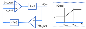
Figure S1: Schematic of the feedback loop for yaw motion control.

The feedback loop is illustrated in Fig. S1. Expressed in the frequency domain, the controlled output of the system is the pendulum angle $\theta(\omega)$. This output is detected with an added angle equivalent imprecision noise $\delta\theta_{\text{imp}}(\omega)$, and fed into a loop filter with a transfer function $G(\omega)$ determining how this signal is converted to an active feedback torque $\tau_{\text{act}}(\omega)$ through the push beam. Additional passive torque noises $\delta\tau_{\text{pas}}(\omega)$ also act on the system. The applied torques turn into a yaw angle through the natural mechanical susceptibility (torque-to-angle transfer function) $\chi(\omega)=(\omega_{0}^{2}-w^{2}+i\omega\gamma(\omega))^{-1}/I$, completing the loop. The passive torques consist of the thermal torque noise, the radiation pressure noise of the probe and push beams, and torques induced by vibration noise around the setup. In the current work, intensity fluctuations are near shot-noise limited, and the resulting total radiation pressure noise is at least three orders of magnitude smaller than thermal noise.

Self-consistency in the loop yields $\theta=\chi(\delta\tau_{\text{pas}}-\tau_{\text{act}})$ with $\tau_{\text{act}}=G(\theta+\delta\theta_{\text{imp}})$. Solving for $\theta$ gives

$$\theta(\omega)=\chi_{\text{eff}}(\omega)\delta\tau_{\text{pas}}(\omega)-\chi_{\text{imp}}(\omega)\delta\theta_{\text{imp}}(\omega),$$ (S6)

where the effective susceptibility is $\chi_{\text{eff}}(\omega)=\frac{\chi(\omega)}{1+G(\omega)\chi(\omega)}$, and the imprecision noise transfer function is $\chi_{\text{imp}}(\omega)=G(\omega)\chi_{\text{eff}}(\omega)$. The dimensionless loop gain $G(\omega)\chi(\omega)$ needs to satisfy the usual stability criteria ($<180^{\circ}$ phase shift at unity loop gain) for the loop to be stable.

The loop transfer function is chosen as that of a variable-gain lead-lag compensation filter (Fig. S1)

$$G(\omega)=\frac{g}{\chi(0)}\frac{1+i\omega/\omega_{\text{lead}}}{1+i\omega/\omega_{\text{lag}}}\approx\frac{g}{\chi(0)}(1+i\frac{\omega}{\omega_{\text{lead}}}).$$ (S7)

Here, $\omega_{\text{lead}}$ and $\omega_{\text{lag}}$ are the start and stop frequencies of the linear gain increase, and the filter gain is chosen such that the DC loop gain $G(0)\chi(0)=g$. The approximation in Eq. S7 is valid for $\omega_{\text{lead}}\ll\omega_{\text{lag}}$. In our experiment, $\omega_{\text{lag}}=2\pi\times 1.5~{}\text{kHz}$ and $\omega_{\text{lead}}=\omega_{\text{eff}}Q_{\text{eff}}(1-\frac{\omega_{0}^{2}}{\omega_{\text{eff}}^{2}})$ has a minimum value of $2\pi\times 7.7~{}\text{Hz}$ for the case of $\omega_{\text{eff}}=2\pi\times 18~{}\text{Hz}$ with critical damping $Q_{\text{eff}}=1/2$, satisfying the approximation well. The unity gain point of the feedback loop needs to come before $\omega_{\text{lag}}$ for loop stability, but the lag part of the filter is needed to make $G(\omega)$ physical since no filter can have an endless gain increase with frequency. Utilizing the parameters in S7, the effective susceptibility $\chi_{\text{eff}}(\omega)$ is given by

$$\begin{split}\chi_{\text{eff}}^{-1}(\omega)&=\chi^{-1}(\omega)+G(\omega)\\ &=I(\omega_{\text{eff}}^{2}-\omega^{2}+i\omega\gamma_{\text{eff}})\end{split}$$ (S8)

where $\omega_{\text{eff}}=\omega_{0}\sqrt{1+g}$ and $\gamma_{\text{eff}}=\frac{\omega_{0}^{2}g}{\omega_{\text{lead}}}+\gamma(\omega)$. Taking into account that $\gamma_{\text{eff}}\gg\gamma(\omega)$ and $\chi(0)=(I\omega_{0}^{2})^{-1}$, Eq. S7 can be rewritten as $G(\omega)=I(\omega_{\text{eff}}^{2})-\omega_{0}^{2}+i\omega\gamma_{\text{eff}}$, resulting into an explicit expression for the imprecision transfer function

$$\chi_{\text{imp}}=\frac{(\omega_{\text{eff}}^{2})-\omega_{0}^{2}+i\omega\gamma_{\text{eff}}}{(\omega_{\text{eff}}^{2})-\omega^{2}+i\omega\gamma_{\text{eff}}}$$ (S9)

Note that all expressions that contain $\gamma_{\text{eff}}$ can also be written in terms of $Q_{\text{eff}}=\frac{\omega_{\text{eff}}}{\gamma_{\text{eff}}}$, which is the primary quantity utilized for the experimental analysis in the main text.

Since all torque and measurement imprecision noises are mutually uncorrelated, the oscillator angular PSD can simply be expressed as

$$S_{\theta\theta}(\omega)=|\chi_{\text{eff}}(\omega)|^{2}S_{\tau\tau}^{\text{pas}}(\omega)+|\chi_{\text{imp}}(\omega)|^{2}S_{\theta\theta}^{\text{imp}}(\omega),$$ (S10)

where the total passive torque PSD $S_{\tau\tau}^{\text{pas}}$ is dominated by the suspension thermal noise with a small contribution from vibrations: $S_{\tau\tau}^{\text{pas}}(\omega)\approx S_{\tau\tau}^{\text{th}}(\omega)+S_{\tau\tau}^{\text{vib}}(\omega)$.

In comparison to a simple change in susceptibility, Eq. S10 shows that the feedback control additionally imprints some detection noise on the oscillation angle PSD. This becomes relatively more important only when the feedback loop tries to control the oscillation amplitude at the measurement noise limit. Eq. S10 forms the basis of the spectral motion analysis under active control in the main text.

.4 Taking under control other pendulum modes

Robust manipulation of the yaw motion requires first taking many other modes of the pendulum under control. In our case, the primary reason for this surfaced when we needed to float the optical table hosting the experiment to reduce ground vibration noise above 5 Hz, such that thermal-noise-limited operation could be achieved. However, floating the table rendered the system unworkable due to the large swing-mode motions it induced. Another limitation was the yaw-motion feedback leading to instabilities in the higher-frequency violin modes of the pendulum.

To circumvent these problems, we mounted the vacuum chamber on the optical table from a single side, forming a cantilever-like structure with natural resonance around 65 Hz. We then actuated (pushed on) the chamber from two orthogonal directions with piezo transducers, gaining the capability of jiggling the pendulum suspension point in space. This led to a configuration where all modes other than the yaw mode were strongly affected by the piezos. The yaw motion was near-purely actuated by the push beam – due to the natural decoupling of torsional motion from suspension point motion. Note that the optical lever system and the QPD were mounted on the rigid optical table, measuring the true motion of the pendulum relative to the massive optical table.

Various levels of information were available on the QPD output for each of the pendulum modes, e.g., longitudinal and horizontal swings at 2.27 Hz, roll at 44.48 Hz, pitch at 125.95 Hz, $1^{st}$ longitudinal and transverse violins at 74.40 Hz and 82.28 Hz, and $2^{nd}$ longitudinal and transverse violins at 169.59 Hz and 178.80 Hz, etc. Note that for an ideal pendulum, no information is expected on the optical lever about the modes that give rise to motion in the transverse direction. However, a 2-degree tilt (from vertical) of the pendulum surface that resulted from a non-ideal gluing of the suspension fiber resulted in all transverse modes imprinting some information on the optical lever.

Each spectral line in the QPD signal was appropriately phase-shifted and amplified with analog electronics and fed back to the relevant piezo transducer to sufficiently dampen the corresponding mechanical mode. Additional details about this far-from-optimal feedback loop are beyond the scope of this article; however, the discussed challenges are not a show stopper for scaling the current setup to more sensitive versions. They just indicate that the vibration isolation architecture needs to be planned in advance to alleviate limitations due to ambient vibrations.

Author contributions

O.H. conceived the experiment and supervised the project. M.M. manufactured the pendulum. S.A. and P.R. built the experimental setup. S.A. and O.H. performed the reported experiments, analyzed the data, and wrote the article.