Grade of membership analysis for multi-layer categorical data

Abstract

Consider a group of individuals (subjects) participating in the same psychological tests with numerous questions (items) at different times. The observed responses can be recorded in multiple response matrices over time, named multi-layer categorical data. Assuming that each subject has a common mixed membership shared across all layers, enabling it to be affiliated with multiple latent classes with varying weights, the objective of the grade of membership (GoM) analysis is to estimate these mixed memberships from the data. When the test is conducted only once, the data becomes traditional single-layer categorical data. The GoM model is a popular choice for describing single-layer categorical data with a latent mixed membership structure. However, GoM cannot handle multi-layer categorical data. In this work, we propose a new model, multi-layer GoM, which extends GoM to multi-layer categorical data. To estimate the common mixed memberships, we propose a new approach, GoM-DSoG, based on a debiased sum of Gram matrices. We establish GoM-DSoG’s per-subject convergence rate under the multi-layer GoM model. Our theoretical results suggest that fewer no-responses, more subjects, more items, and more layers are beneficial for GoM analysis. We also propose an approach to select the number of latent classes. Extensive experimental studies verify the theoretical findings and show GoM-DSoG’s superiority over its competitors, as well as the accuracy of our method in determining the number of latent classes.

1 Introduction

Categorical data is extensively collected in psychological tests, educational assessments, and political surveys [28, 1, 5, 27]. This type of data typically comprises responses from subjects to a set of items and is often represented by an $N\times J$ observed response matrix $R$, where $N$ denotes the number of subjects (individuals) participating in the test and $J$ represents the number of items (questions). In this matrix, $R(i,j)$ signifies the response of subject $i$ to item $j$. When each item has only two choices (e.g., yes/no choices or right/wrong answers), the data is referred to as categorical data with binary responses. In this case, $R\in\{0,1\}^{N\times J}$, where $0$ and $1$ are used to indicate the binary choices. When each item has $M$ ($M\geq 3$) choices, the data is known as categorical data with polytomous responses. For such data, $R\in\{0,1,\ldots,M\}^{N\times J}$, where $0$ typically represents no response (missing response). It is evident that polytomous responses are more general than binary responses, and thus, this paper focuses on polytomous responses. A key characteristic of traditional categorical data is that it is often collected only once for each subject, resulting in a single-layer categorical dataset. For such data, learning the latent classes (subgroups) of subjects is often of great interest, as subjects with similar subgroup information typically exhibit similar response patterns. Specifically, the task of learning subjects’ latent classes is known as latent class analysis (LCA) [12, 21], where the latent classes can be different personalities, abilities, and political ideologies in psychological tests, educational assessments, and political surveys [4], respectively. Therefore, equipped with LCA, categorical data plays a key role in understanding human behaviors, preferences, and attitudes.

However, despite its prevalence, the single-layer structure of traditional categorical data inherently limits the depth of analysis that can be performed, as it captures only a snapshot of the subjects’ responses at a single point in time. In many practical scenarios, the same group of subjects may be assessed multiple times over different time points using the same set of items. This repeated assessment generates multi-layer categorical data, with each layer representing a different time point. For such data, all layers share common subjects and items, creating a longitudinal dataset rich in information. The additional temporal dimension offered by multi-layer categorical data provides a more comprehensive view of subjects’ responses, potentially revealing patterns and trends that are not discernible in single-layer categorical data.

For single-layer categorical data, a popular statistical model for describing its latent class structure is the latent class model (LCM) [9], which operates under the assumption that each subject is assigned to a single latent class. However, the non-overlapping classes property of LCM can be restrictive, potentially failing to fully capture the complexity and diversity of subjects’ response patterns. The grade of membership (GoM) model [31] overcomes LCM’s limitation and allows each subject to belong to at least one latent class, providing a more powerful modeling capacity than LCM. Existing approaches for learning subjects’ latent mixed memberships in single-layer categorical data modeled by the GoM encompass Bayesian inference utilizing MCMC [6, 10, 11], joint maximum likelihood algorithms [26], and spectral methods [4, 23].

However, all the above methods are inherently limited to single-layer categorical data and cannot be directly applied to learning the common latent classes of subjects in multi-layer categorical data. The additional temporal dimension in multi-layer categorical data introduces new challenges and opportunities for latent class analysis. Recently, to describe the latent class structures in multi-layer categorical data, [24] proposed a multi-layer LCM which assumes that each subject belongs to only one latent subgroup. [24] also provides several spectral methods with theoretical guarantees to discover the latent classes of subjects. However, one main limitation of the multi-layer LCM is that it cannot model multi-layer categorical data with a latent mixed membership structure, where each subject can belong to different subgroups with varying weights.

To address the limitations of the aforementioned models and methods for multi-layer categorical data with a latent mixed membership structure, this work introduces the multi-layer grade of membership (multi-layer GoM) model, which extends the traditional GoM model to multi-layer categorical data. This extension enables us to capture the temporal dynamics of subject responses provided by multiple layers and allows subjects to belong to more than one latent class simultaneously. For the estimation of the common mixed memberships, we develop a novel approach, GoM-DSoG, based on a debiased sum of Gram matrices. This approach effectively handles the challenges posed by multi-layer data. We also establish the per-subject convergence rate of GoM-DSoG under the proposed model. Our theoretical and experimental results highlight the benefits of considering more layers than a single layer in the task of grade of membership analysis for categorical data. In particular, if there are too many non-responses in the categorical data with polytomous responses or too many zeros in the categorical data with binary responses, more tests should be considered, and our GoM-DSoG is an efficient tool to estimate subjects’ common mixed memberships for such multi-layer categorical data. Additionally, an approach for selecting the number of latent classes $K$ in multi-layer categorical data generated from the proposed model is developed. By conducting substantial experimental studies, we empirically verify the theoretical results and show the superiority of the proposed GoM-DSoG method over its competitors and the high accuracy of our method in choosing $K$.

Notation: $I_{m\times m}$ and $[m]$ represent the $m\times m$ identity matrix and set $\{1,2,\ldots,m\}$, respectively. For any matrix $H$, $H^{\prime}$ denotes its transpose, $H(s,:)$ denotes its submatrix for rows in the set $s$, $\|H\|_{1}$ is its the $l_{1}$ norm, $\|H\|_{F}$ represents its Frobenius norm, $\|H\|$ means its spectral norm, $\|H\|_{\infty}$ represents its maximum absolute row sum, $\|H\|_{2\rightarrow\infty}$ denotes its maximum row-wise $l_{2}$ norm, $\lambda_{k}(H)$ denotes its $k$-th largest eigenvalue in magnitude, and $\mathrm{rank}(H)$ denotes its rank. $e_{i}$ is a vector satisfying $e_{i}(i)=1$ and $e_{i}(j)=0$ for $j\neq i$. $\mathbb{E}(\cdot)$ denotes expectation and $\mathbb{P}(\cdot)$ represents probability.

We organize the remainder of this paper as follows. We introduce our model in Section 2. Our method for fitting proposed model and its theoretical guarantees are presented in Section 3. Section 4 proposes an approach for determining $K$. Section 5 conducts experimental studies. Section 6 concludes the paper.

2 Multi-layer grade of membership model

Suppose that all subjects belong to $K$ common latent classes, denoted as:

$$\mathcal{C}_{1},\mathcal{C}_{2},\ldots,\mathcal{C}_{K}.$$ (1)

We assume that $K$ is known in this paper and we will also propose an approach for selecting $K$ in Section 4. The memberships of subjects belonging to different latent classes can be characterized by a common membership matrix $\Pi\in[0,1]^{N\times K}$ shared across all layers, where:

$$\Pi(i,k)\text{ is the ``weight'' for the partial membership of subject }i\text{~{}on~{}}\mathcal{C}_{k},\quad i\in[N],k\in[K].$$ (2)

By $\Pi$’s definition, for $i\in[N]$, we have $\sum_{k\in[K]}\Pi(i,k)=1$. Call subject $i$ pure if one entry of $\Pi(i,:)$ equals 1, and mixed otherwise. In this paper, we assume that:

$$\text{There is at least one pure subject in each latent class}.$$ (3)

Combining Equations (2) and (3) implies that $\Pi$ is full rank, and its rank is $K$ since we assume $K\ll\mathrm{min}(N,J)$ in this paper. Let $p_{k}$ denote the index of any pure subject in the $k$-th latent class $\mathcal{C}_{k}$ for $k\in[K]$. Define the pure subject index set $\mathcal{I}$ as $\mathcal{I}=\{p_{1},p_{2},\ldots,p_{K}\}$. Without loss of generality, similar to the analysis in [17], reorder all subjects such that $\Pi(\mathcal{I},:)=I_{K\times K}$.

For each layer $l\in[L]$, let $\Theta_{l}\in[0,M]^{J\times K}$ denote the item parameter matrix of the $l$-th layer categorical data. Our model, a multi-layer extension of the classical GoM model, is formally defined as follows.

Definition 1.

(Multi-layer grade of membership model) Let $R_{l}\in\{0,1,\ldots,M\}^{N\times J}$ represent the observed response matrix of the $l$-th layer categorical data for $l\in[L]$. Our multi-layer grade of membership (multi-layer GoM) model for generating the $L$ observed response matrices $\{R_{l}\}_{l=1}^{L}$ is defined as:

$$\mathscr{R}_{l}:=\Pi\Theta^{\prime}_{l},\quad\text{where }R_{l}(i,j)\sim\text{Binomial}(M,\frac{\mathscr{R}_{l}(i,j)}{M}),\quad i\in[N],j\in[J],l\in[L].$$ (4)

For convenience, call $\mathscr{R}_{l}$ the $l$-th population response matrix since $\mathbb{E}(R_{l})=\mathscr{R}_{l}$ for $l\in[L]$ under the Binomial distribution. When all subjects are pure, our model degenerates the multi-layer LCM introduced in [24]. When the number of layers $L$ equals 1, the multi-layer GoM defined by Equation (4) simplifies to the GoM model for single-layer categorical data considered in [23]. Furthermore, when both $L=1$ and $M=1$, the proposed model reduces to the GoM model studied in [4].

Equation (4) necessitates that the elements of $\Theta_{l}$ range within $[0,M]$ for $l\in[L]$ because $\frac{\mathscr{R}_{l}(i,j)}{M}$ represents a probability within $[0,1]$, and $\Pi$ satisfies Equation (2). By the definition of multi-layer GoM, at the $l$-th layer, the probability that subject $i$ selects the $m$-th choice in item $j$ equals

$$\mathbb{P}(R_{l}(i,j)=m)=\frac{M!}{m!(M-m)!}(\frac{\mathscr{R}_{l}(i,j)}{M})^{m}(1-\frac{\mathscr{R}_{l}(i,j)}{M})^{M-m},\qquad m=0,1,\ldots,M.$$ (5)

Using Equation (4), our multi-layer GoM can generate $\{R_{l}\}^{L}_{l=1}$ with a latent true membership matrix $\Pi$ and item parameter matrices $\{\Theta_{l}\}^{L}_{l=1}$. This paper aims to recover $\Pi$ and $\{\Theta_{l}\}^{L}_{l=1}$ given the $L$ observed response matrices $\{R_{l}\}^{L}_{l=1}$.

2.1 Sparsity scaling

In real-world multi-layer categorical data with polytomous responses, some no-responses (0s) may exist. Specifically, for multi-layer categorical data with binary responses when $M=1$, we have $R_{l}\in\{0,1\}^{N\times J}$ for $l\in[L]$, which may result in numerous zeros in the data, although zero does not signify a no-response for binary responses. A large number of no-responses (0s) in the dataset poses a significant challenge for the task of grade of membership analysis. Therefore, it is crucial to control the number of zeros in the multi-layer categorical data. Define $\rho=\mathrm{max}_{l\in[L]}\mathrm{max}_{j\in[J],k\in[K]}\Theta_{l}(j,k)$ and $B_{l}=\frac{\Theta_{l}}{\rho}$ for $l\in[L]$. Given that $\Theta_{l}\in[0,M]^{J\times K}$, it follows that $\rho\in(0,M]$, the maximum element of $B_{l}$ is no larger than 1, and $\mathscr{R}_{l}(i,j)\leq\rho$ for $i\in[N],j\in[J],l\in[L]$. According to Equation (5), we have:

$$\mathbb{P}(R_{l}(i,j)=0)=(1-\frac{\mathscr{R}_{l}(i,j)}{M})^{M}=(1-\frac{\rho\Pi(i,:)B^{\prime}_{l}(j,:)}{M})^{M},$$

which indicates that increasing $\rho$ decreases the probability of generating no-responses across all layers. Consequently, $\rho$ serves as a controlling factor for the overall sparsity of the data, thus justifying its designation as the sparsity parameter. To thoroughly examine the performance of the proposed method under varying levels of data’s sparsity, we will permit $\rho$ to approach zero and incorporate it into the error bound for further analysis.

3 Debiased spectral method and its theoretical guarantees

We propose an efficient method for $\Pi$ and $\{\Theta_{l}\}^{L}_{l=1}$ in this section. Subsequently, we establish its theoretical guarantees under the multi-layer GoM model.

3.1 Debiased spectral method

Suppose that the population response matrices $\{\mathscr{R}_{l}\}^{L}_{l=1}$ are observed, and our objective is to accurately recover $\Pi$ and $\{\Theta_{l}\}^{L}_{l=1}$ from $\{\mathscr{R}_{l}\}^{L}_{l=1}$. Define $\mathcal{S}=\sum_{l=1}^{L}\mathscr{R}_{l}\mathscr{R}^{\prime}_{l}$, where $\mathcal{S}$ is a symmetric matrix and it represents an aggregation of $L$ Gram matrices $\{\mathscr{R}_{l}\mathscr{R}^{\prime}_{l}\}^{L}_{l=1}$. The following proposition guarantees the identifiability of our multi-layer GoM model.

Proposition 1.

(Identifiability). Assume that $\mathrm{rank}(\sum_{l=1}^{L}\Theta^{\prime}_{l}\Theta_{l})=K$. Then, our multi-layer GoM model is identifiable: For any $(\Pi,\{\Theta_{l}\}^{L}_{l=1})$ and $(\tilde{\Pi},\{\tilde{\Theta}_{l}\}^{L}_{l=1})$, if $\Pi\Theta^{\prime}_{l}=\tilde{\Pi}\tilde{\Theta}^{\prime}_{l}$ for $l\in[L]$, we have $\tilde{\Pi}=\Pi\mathcal{P}$ and $\tilde{\Theta}_{l}=\Theta_{l}\mathcal{P}$ for $l\in[L]$, where $\mathcal{P}$ is a permutation matrix.

The identifiability proposed in Proposition 1 guarantees that our multi-layer GoM is well-defined since the model parameters $(\Pi,\{\Theta_{l}\}^{L}_{l=1})$ can be uniquely recovered up to a permutation. The intuition of the proposed method comes from the following lemma.

Lemma 1.

When $\mathrm{rank}(\sum_{l=1}^{L}\Theta^{\prime}_{l}\Theta_{l})=K$, let $\mathcal{S}=U\Lambda U^{\prime}$ denote the leading $K$ eigendecomposition of $\mathcal{S}$, where $U^{\prime}U=I_{K\times K}$. Then, we have:

• $U=\Pi U(\mathcal{I},:)$,

• $\Theta_{l}=\mathscr{R}^{\prime}_{l}\Pi(\Pi^{\prime}\Pi)^{-1}$ for $l\in[L]$.

Given that the summation of each row of $\Pi$ equals 1 and $\Pi$ satisfies Equation (3), the form $U=\Pi U(\mathcal{I},:)$ is known as the Ideal Simplex (IS), where $U(\mathcal{I},:)$’s $K$ rows are the $K$ vertexes in the simplex structure. A similar Ideal Simplex is also discovered in the field of mixed membership community detection in network science [17, 13, 25], grade of membership analysis for single-layer categorical data [4, 23], and topic modeling [15, 14].

Since $U(\mathcal{I},:)$ is non-singular, we have $\Pi=UU^{-1}(\mathcal{I},:)$ by $U=\Pi U(\mathcal{I},:)$. This implies that $\Pi$ can be exactly recovered if we can obtain $U(\mathcal{I},:)$ from the $N\times K$ eigenvector matrix $U$. Similar to previous works related to the IS structure, the successive projection algorithm (SPA) [2, 7, 8] can be employed to precisely identify the $K$ vertices $U(\mathcal{I},:)$ within $U$, leveraging the simplex structure $U=\Pi U(\mathcal{I},:)$. SPA is a widely used technique for vertex hunting. Once we obtain $\Pi$, we can recover $\{\Theta_{l}\}^{L}_{l=1}$ using the second result of Lemma 1. To adapt this idea to the real case, we set $H=\mathrm{max}(0,UU^{-1}(\mathcal{I},:))\equiv\Pi$, ensuring that $\Pi(i,:)=\frac{H(i,:)}{\|H(i,:)\|_{1}}$ and $\Theta_{l}=\mathscr{R}^{\prime}_{l}\Pi(\Pi^{\prime}\Pi)^{-1}$ for $i\in[N],l\in[L]$.

For real data, the $L$ response matrices $\{R_{l}\}^{L}_{l=1}$ are observed, while their expectations $\{\mathscr{R}_{l}\}^{L}_{l=1}$ are not available. For each $l\in[L]$, let $D$ be an $N\times N$ diagonal matrix with $D_{l}(i,i)=\sum_{j\in[J]}R_{l}^{2}(i,j)$ for $i\in[N]$. Define $S=\sum_{l\in[L]}(R_{l}R_{l}^{\prime}-D_{l})$, where $S$ is known as the debiased sum of Gram matrices [29]. Let $\hat{U}\hat{\Lambda}\hat{U}^{\prime}$ be the leading $K$ eigendecomposition of $S$, where $\hat{U}^{\prime}\hat{U}=I_{K\times K}$. It is known that the $N\times N$ symmetric matrix $S$ is a debiased estimator of $\mathcal{S}$, while $\sum_{l\in[L]}R_{l}R_{l}^{\prime}$ is a biased estimator, following similar analysis as in [16, 29]. Therefore, let $\hat{\mathcal{I}}$ represent the estimated pure subjects’ index set found by employing SPA to $\hat{U}$ with $K$ vertices. Define $\hat{H}=\max(0,\hat{U}\hat{U}^{-1}(\hat{\mathcal{I}},:))$, let $\hat{\Pi}$ be an $N\times K$ matrix such that $\hat{\Pi}(i,:)=\frac{\hat{H}(i,:)}{\|\hat{H}(i,:)\|_{1}}$ for $i\in[N]$, and define $\hat{\Theta}_{l}=R_{l}^{\prime}\hat{\Pi}(\hat{\Pi}^{\prime}\hat{\Pi})^{-1}$ for $l\in[L]$. We see that $\hat{\Pi}$ and $\{\hat{\Theta}_{l}\}^{L}_{l=1}$ are good estimations of $\Pi$ and $\{\Theta_{l}\}^{L}_{l=1}$, respectively. The above analysis is summarized in Algorithm 1.

Algorithm 1 Grade of Membership analysis via the Debiased Sum of Gram matrices (GoM-DSoG)

1:The $L$ observed response matrices $R_{1},R_{2},\ldots,R_{L}$ and the number of latent classes $K$, where $R_{l}\in\{0,1,2,\ldots,M\}^{N\times J}$ for $l\in[L]$.

2:Estimated membership matrix $\hat{\Pi}$ and estimated item parameter matrices $\{\hat{\Theta}_{l}\}^{L}_{l=1}$.

3:Calculate $S=\sum_{l\in[L]}(R_{l}R_{l}^{\prime}-D_{l})$, where $D_{l}$ is a diagonal matrix with $D_{l}(i,i)=\sum_{j\in[J]}R_{l}^{2}(i,j)$ for $i\in[N],l\in[L]$.

4:Compute $\hat{U}\hat{\Lambda}\hat{U}^{\prime}$, the leading $K$ eigendecomposition of $S$.

5:Apply SPA to $\hat{U}$ assuming that there are $K$ vertices to get the estimated pure subjects’ index set $\hat{\mathcal{I}}$.

6:Set $\hat{H}=\mathrm{max}(0,\hat{U}\hat{U}^{-1}(\hat{\mathcal{I}},:))$.

7:For $i\in[N]$, set $\hat{\Pi}(i,:)=\frac{\hat{H}(i,:)}{\|\hat{H}(i,:)\|_{1}}$.

8:For $l\in[L]$, set $\hat{\Theta}_{l}=R_{l}^{\prime}\hat{\Pi}(\hat{\Pi}^{\prime}\hat{\Pi})^{-1}$.

3.2 Consistency results

This subsection presents the theoretical findings exploring the advantages of multi-layer categorical data over single-layer categorical data for grade of membership analysis. We investigate the asymptotic consistency of GoM-DSoG under the proposed multi-layer GoM model across different sparsity levels. Specifically, we assume that $N$, $J$, and $L$ can approach infinity in the asymptotic setting, with no assumed relationship among their growth rates. Before presenting the main result, we outline some assumptions.

We consider the asymptotic regime in which $N$, $J$, and $L$ approach infinity.

Assumption 1.

$\rho^{2}NJL\gg\mathrm{log}(N+J+L)$.

Since $N$, $J$, and $L$ can grow to infinity in our analysis, Assumption 1 is mild, as it implies that $\rho$ should be significantly larger than $\sqrt{\frac{\log(N+J+L)}{NJL}}$ (therefore, $\rho$ can be sufficiently small for large values of $N$, $J$, and $L$). This assumption imposes a lower bound on $\rho$, indicating that there cannot be too many no-responses in the multi-layer categorical data. It is worth noting that when $J=O(N)$, our Assumption 1 is in agreement with the sparsity requirement stated in Theorem 1 of [16]. This alignment is expected since both our GoM-DSoG and the Bias-adjusted SoS algorithm provided in [16] are debiased spectral clustering methods.

Assumption 2.

$|\lambda_{K}(\sum_{l\in[L]}B^{\prime}_{l}B_{l})|\geq c_{1}JL$ for some positive constant $c_{1}$.

This assumption requires a linear growth of $|\lambda_{K}(\sum_{l\in[L]}B^{\prime}_{l}B_{l})|$ concerning the number of layers $L$ and it serves a similar purpose in our theoretical analysis as the second point of Assumption 1 in [16], Assumption 2 in [29], and the last point of Condition 2 in [4].

Condition 1.

$K=O(1)$ and $\lambda_{K}(\Pi^{\prime}\Pi)=O(\frac{N}{K})$.

This condition serves a similar purpose to the first point of Assumption 1 in [16], Condition 2 in [4], Assumption 1 in [29], and so on. It is necessary to simplify our theoretical analysis.

Theorem 1 presents our main result for the task of grade membership analysis. It provides the per-node error rate of the proposed algorithm. To obtain Theorem 1, we first bound $\|S-\mathcal{S}\|_{\infty}$ using the Bernstein inequality provided in [30]. Subsequently, we utilize this bound to establish a bound for the row-wise eigenvector error $\|\hat{U}\hat{U}^{\prime}-UU^{\prime}\|_{2\rightarrow\infty}$ based on Theorem 4.2 of [3].

Theorem 1.

Consider a multi-layer GoM parameterized by $\{\Pi,\{\Theta_{l}\}^{L}_{l=1}\}$. Under the assumptions of 1, 2, and the condition 1, with high probability, we have

$$\max_{i\in[N]}\|e^{\prime}_{i}(\hat{\Pi}-\Pi\mathcal{P})\|_{1}=O(\sqrt{\frac{\log(N+J+L)}{\rho^{2}NJL}})+O(\frac{1}{N}).$$

The result presented in Theorem 1 indicates that enhancing the values of $\rho$, $N$, and $J$ enhances the performance of GoM-DSoG in estimating $\Pi$, which aligns with our intuition. Moreover, it indicates that as $L$ increases, GoM-DSoG demonstrates improved performance for the task of GoM analysis. This observation underscores the benefits of considering multi-layer categorical data over single-layer categorical data, as the former contains more responses and, consequently, more information.

For the task of estimating the item parameter matrices $\{\Theta_{l}\}^{L}_{l=1}$, the following lemma provides a bound on $\frac{\|\sum_{l\in[L]}(\hat{\Theta}_{l}-\Theta_{l}\mathcal{P})\|_{F}}{\|\sum_{l\in[L]}\Theta_{l}\|_{F}}$.

Lemma 2.

Consider a multi-layer GoM parameterized by $\{\Pi,\{\Theta_{l}\}^{L}_{l=1}\}$. Under the conditions that $\rho L\mathrm{max}(N,J)\gg\mathrm{log}(N+J+L)$ and $|\lambda_{1}(\sum_{l\in[L]}B_{l})|\geq c_{2}\sqrt{J}L$ for some constant $c_{2}>0$, with high probability, we have

$$\frac{\|\sum_{l\in[L]}(\hat{\Theta}_{l}-\Theta_{l}\mathcal{P})\|_{F}}{\|\sum_{l\in[L]}\Theta_{l}\|_{F}}=O(\sqrt{\frac{\mathrm{max}(N,J)\mathrm{log}(N+J+L)}{\rho NJL}}).$$

Note that the conditions specified in Lemma 2 differ from those of Theorem 1. This difference arises because bounding $\|\sum_{l\in[L]}(R_{l}-\mathscr{R}_{l})\|$ is necessary to obtain the result presented in Lemma 2. Despite the distinct conditions, the result in Lemma 2 also indicates that enhancing the values of $\rho,N,J$, and $L$ leads to improved performance of the GoM-DSoG method.

4 Estimation of $K$

Selecting the appropriate number of latent classes $K$ in multi-layer categorical data with a latent mixed membership structure poses a significant challenge. While Algorithm 1 assumes $K$ is known, this is often not feasible in practical applications. Given $L$ observed responses $\{R_{l}\}^{L}_{l=1}$, our GoM-DSoG algorithm can always produce an estimated mixed membership matrix $\hat{\Pi}_{k}\in[0,1]^{N\times k}$ for any number of latent classes $k$. When faced with multiple potential choices for $K$, such that the true $K$ may be one of $\{1,2,\ldots,K_{c}\}$, we can run our GoM-DSoG algorithm on the data with $k$ latent classes for all $k\in[K_{c}]$, resulting in $K_{c}$ estimated mixed membership matrices $\{\hat{\Pi}_{k}\}^{K_{c}}_{k=1}$. Naturally, this leads to the question of which estimated membership matrix indicates the best quality of mixed membership partition.

To address this question, we propose a metric called averaged fuzzy modularity, inspired by the fuzzy modularity introduced in [23] for single-layer categorical data with a latent mixed membership structure. The averaged fuzzy modularity based on the estimated mixed membership matrix $\hat{\Pi}_{k}$ when we assume there are $k$ latent classes is defined as follows:

$$Q(\hat{\Pi}_{k})=\frac{1}{L}\sum_{l\in[L]}\sum_{i\in[N]}\sum_{j\in[N]}\frac{1}{\eta_{l}}(G_{l}(i,j)-\frac{g_{l}(i,i)g_{l}(j,j)}{\eta_{l}})\hat{\Pi}_{k}(i,:)\hat{\Pi}^{\prime}_{k}(j,:),$$ (6)

where $G_{l}=R_{l}R^{\prime}_{l}$, $g_{l}$ is an $N\times N$ diagonal matrix with $g_{l}(i,i)=\sum_{j\in[N]}G_{l}(i,j)$, and $\eta_{l}=\sum_{j\in[N]}g_{l}(j,j)$ for $i\in[N],l\in[L]$. This metric has several notable properties:

• When there are no mixed subjects, our modularity reduces to the averaged modularity of [22, 24].

• When $L=1$, it reduces to the fuzzy modularity of [18, 23].

• When $L=1$ and there are no mixed subjects, it becomes the popular Newman-Girvan modularity [20].

A larger value of $Q$ indicates better quality of mixed membership partition [19, 18, 22]. Therefore, similar to [18], we infer the optimal $K$ by choosing the one that maximizes $Q$ defined in Equation (6).

5 Experimental studies

This part investigates the performance of the proposed GoM-DSoG method for the task of the grade of membership analysis and its accuracy in the estimation of $K$. To this end, we conduct five experiments to study the effects of various factors, including the number of subjects $N$, the number of layers $L$, the sparsity parameter $\rho$, the number of pure subjects in each latent class, and the number of latent classes $K$. In all experiments, the GoM-DSoG method is compared with the following two different algorithms:

• GoM-Sum: Set $R_{\mathrm{sum}}=\sum_{l\in[L]}R_{l}$. Let $\hat{U}_{R_{\mathrm{sum}}}\hat{\Sigma}_{R_{\mathrm{sum}}}\hat{V}^{\prime}_{R_{\mathrm{sum}}}$ represent $R_{\mathrm{sum}}$’s leading $K$ singular value decomposition, where $\hat{U}^{\prime}_{R_{\mathrm{sum}}}\hat{U}_{R_{\mathrm{sum}}}=I_{K\times K}$. This approach estimates the parameters $\Pi$ and $\{\Theta_{l}\}^{N}_{l=1}$ by substituting $R_{\mathrm{sum}}$ for $S$ and $\hat{U}_{R_{\mathrm{sum}}}$ for $\hat{U}$ in Algorithm 1.

• GoM-SoG: Set $\tilde{S}=\sum_{l\in[L]}R_{l}R^{\prime}_{l}$. This method estimates $\Pi$ and $\{\Theta_{l}\}^{N}_{l=1}$ by replacing $S$ with $\tilde{S}$ in Algorithm 1.

Remark 1.

Define $\mathscr{R}_{\mathrm{sum}}=\sum_{l\in[L]}\mathscr{R}_{l}$. When the rank of the $J\times K$ aggregation matrix $\sum_{l\in[L]}B_{l}$ is $K$, let $U_{\mathscr{R}_{\mathrm{sum}}}\Sigma_{\mathscr{R}_{\mathrm{sum}}}V^{\prime}_{\mathscr{R}_{\mathrm{sum}}}$ denote the leading $K$ singular value decomposition of $\mathscr{R}_{\mathrm{sum}}$ such that $U^{\prime}_{\mathscr{R}_{\mathrm{sum}}}U_{\mathscr{R}_{\mathrm{sum}}}=I_{K\times K}$. The intuition behind GoM-Sum stems from the observation that $U_{\mathscr{R}_{\mathrm{sum}}}=\Pi U_{\mathscr{R}_{\mathrm{sum}}}(\mathcal{I},:)$ also exhibits a simplex structure. The intuition behind GoM-SoG is analogous to that of GoM-DSoG, as $\tilde{S}$ serves as a biased estimator of $\mathcal{S}$ [16, 29, 24]. By following a similar analysis as in [24], we can obtain theoretical guarantees for GoM-Sum and GoM-SoG. Furthermore, we can prove that our proposed GoM-DSoG consistently outperforms both GoM-Sum and GoM-SoG. For brevity, we omit the detailed theoretical analysis of GoM-Sum and GoM-SoG in this paper.

To assess the performance of all approaches in estimating $\Pi$, the Relative $l_{1}$ error defined as $\mathrm{min}_{\mathcal{P}\in\mathcal{X}}\frac{\|\hat{\Pi}-\Pi\mathcal{P}\|_{1}}{N}$ is used, where $\mathcal{X}$ collects all $K\times K$ permutation matrices. To measure their performances in estimating $\{\Theta_{l}\}^{L}_{l=1}$, we use the Relative $l_{2}$ error, defined as $\mathrm{min}_{\mathcal{P}\in\mathcal{X}}\frac{\|\sum_{l\in[L]}(\hat{\Theta}_{l}-\Theta_{l}\mathcal{P})\|_{F}}{\|\sum_{l\in[L]}\Theta_{l}\|_{F}}$. To evaluate the accuracy of all methods in estimating $K$, the Accuracy rate calculated by the proportion of times an approach accurately chooses the true $K$ by maximizing $Q$ is employed. The Relative $l_{1}$ error and Relative $l_{2}$ error metrics are such that smaller values are better, while the Accuracy rate metric is such that larger values are better.

For all experiments, we set $J=\frac{N}{5}$ and $M=5$, so that $R_{l}\in\{0,1,2,3,4,5\}^{N\times\frac{N}{5}}$ for all $l\in[L]$. Let each latent class have $N_{0}$ pure subjects. For a mixed subject $i$, set $\Pi(i,k)=\frac{\mathrm{rand}(1)}{K-1}$ for $k\in[K-1]$ and $\Pi(i,K)=1-\sum_{k\in[K-1]}\Pi(i,k)$ when $K\geq 2$, where $\mathrm{rand}(1)$ denotes a random value from $(0,1)$. For $j\in[J],k\in[K],l\in[L]$, set $B_{l}(j,k)=\mathrm{rand}(1)$. For all experiments, $N,K,\rho,N_{0}$, and $L$ are set independently. For each parameter setting, we report the averaged metric over the 50 repetitions. For all approaches, $K$ is given for estimating $\Pi$ and $\{\Theta_{l}\}^{L}_{l=1}$ while $K$ is not given and is estimated by maximizing the averaged fuzzy modularity value $Q$ for the task of determining $K$. Meanwhile, for each experiment, there are two cases: the sparse case and the dense case. In the sparse case, we let the sparsity parameter $\rho$ be small, while in the dense case, $\rho$ is large. The sparse case is characterized by numerous zeros in the generated data, which aligns multi-layer categorical data with binary responses or the scenario where many participants do not respond to all items in each test. Conversely, the dense case features only a few non-responses, corresponding to real-world situations where only a minority of participants have non-responses in multi-layer categorical data with polytomous responses.

Experiment 1: Effect of changing $N$. Set $L=5$, $N_{0}=N/5$, and $K=3$. Let $N$ vary in $\{100,200,\ldots,1000\}$. For the sparse case, set $\rho=0.2$. For the dense case, set $\rho=5$. Results are presented in Figure 1, indicating that (a) all methods enjoy better performance as the number of subjects $N$ grows; (b) our GoM-DSoG slightly outperforms GoM-SoG, and both methods significantly outperform GoM-Sum, especially in the sparse case; (c) all methods perform better in the dense case compared to the sparse case for estimating $\Pi$, $\{\Theta_{l}\}^{L}_{l=1}$, and $K$. Notably, all methods demonstrate satisfactory performance in the dense case, which is consistently observed in other experiments (thus, similar analyses are omitted for subsequent experiments).

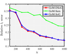
(a) $\rho=0.2$

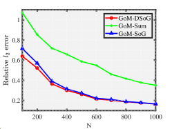
(b) $\rho=0.2$

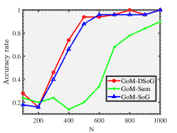
(c) $\rho=0.2$

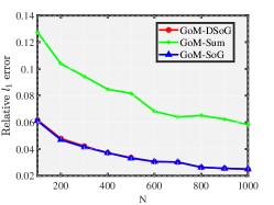
(d) $\rho=5$

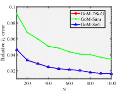
(e) $\rho=5$

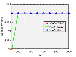
(f) $\rho=5$

Figure 1: Experiment 1.

Experiment 2: Effect of changing $L$. Set $N=500$, $N_{0}=100$, and $K=3$. Let $L$ vary in $\{1,2,\ldots,10\}$. For the sparse case, set $\rho=0.2$. For the dense case, set $\rho=5$. Results are reported in Figure 2. Observations include that GoM-DSoG and GoM-SoG perform similarly, both methods behave better as $L$ increases, and they consistently outperform GoM-Sum. The results of this experiment support the advantages of considering multiple tests at different times. Specifically, if a significant proportion of no-responses is present in the data, conducting additional tests at various times, i.e., increasing $L$, can be beneficial. This process results in multi-layer categorical data. However, for such data, simply summing all response matrices (i.e., using the GoM-Sum method) for the grade of membership analysis and estimating $K$ is inefficient. Instead, our proposed GoM-DSoG method is more effective.

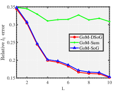
(a) $\rho=0.2$

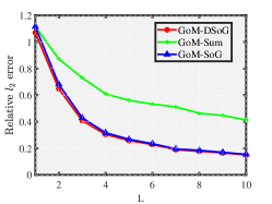
(b) $\rho=0.2$

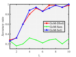
(c) $\rho=0.2$

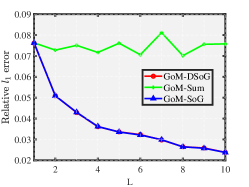
(d) $\rho=5$

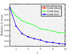
(e) $\rho=5$

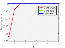
(f) $\rho=5$

Figure 2: Experiment 2.

Experiment 3: Effect of changing $\rho$. Set $N=500$, $L=5$, $N_{0}=100$, and $K=3$. For the sparse case, let $\rho$ vary in $\{0.05,0.1,\ldots,0.5\}$. For the dense case, let $\rho$ vary in $\{0.5,1,\ldots,5\}$. Results are displayed in Figure 3. Observations indicate that all methods perform better as the sparsity parameter $\rho$ increases, our GoM-DSoG slightly outperforms GoM-SoG, and both significantly outperform GoM-Sum.

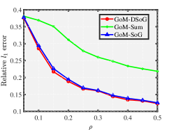
(a) $\rho\in\{0.05,0.1,\ldots,0.5\}$

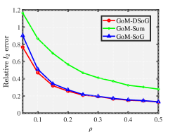
(b) $\rho\in\{0.05,0.1,\ldots,0.5\}$

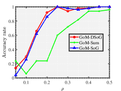
(c) $\rho\in\{0.05,0.1,\ldots,0.5\}$

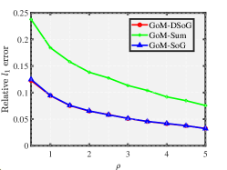
(d) $\rho\in\{0.5,1,\ldots,5\}$

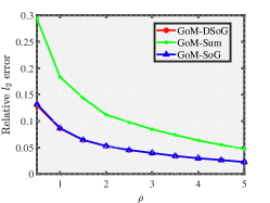
(e) $\rho\in\{0.5,1,\ldots,5\}$

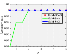
(f) $\rho\in\{0.5,1,\ldots,5\}$

Figure 3: Experiment 3.

Experiment 4: Effect of changing $N_{0}$. Set $N=600$, $L=10$, and $K=3$. Let $N_{0}$ vary in $\{20,40,\ldots,200\}$. For the sparse case, set $\rho=0.2$. For the dense case, set $\rho=5$. Performances of the three methods are reported in Figure 4. Results suggest that all methods exhibit improved performance in estimating the item parameter matrices and $K$ when $N_{0}$ grows, with GoM-DSoG performing slightly better than GoM-SoG and both significantly outperforming GoM-Sum.

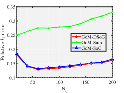
(a) $\rho=0.2$

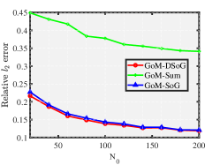
(b) $\rho=0.2$

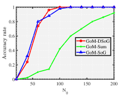
(c) $\rho=0.2$

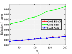
(d) $\rho=5$

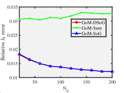
(e) $\rho=5$

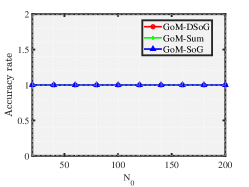
(f) $\rho=5$

Figure 4: Experiment 4.

Experiment 5: Effect of changing $K$. Set $N=100K,N_{0}=N/K,L=5$. Let $K$ vary in $\{1,2,\ldots,8\}$. For the sparse case, set $\rho=0.5$. For the dense case, set $\rho=5$. Results are summarized in Figure 5. Observations include that (a) GoM-DSoG and GoM-SoG significantly outperform GoM-Sum in the dense case; (b) all methods fail to estimate $K$ when the true $K$ is 1. However, this is not a critical issue since we typically assume that there are at least 2 latent classes for the task of grade of membership analysis.

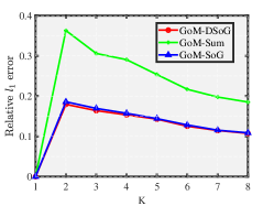
(a) $\rho=0.5$

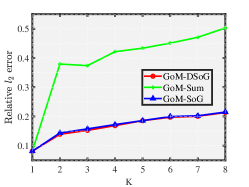
(b) $\rho=0.5$

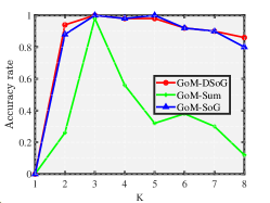
(c) $\rho=0.5$

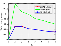
(d) $\rho=5$

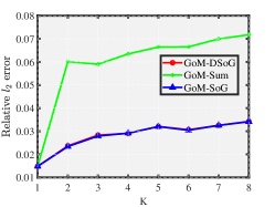
(e) $\rho=5$

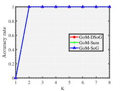
(f) $\rho=5$

Figure 5: Experiment 5.

6 Conclusion

In this paper, we propose a novel model, the multi-layer GoM model, which extends the traditional GoM model to effectively describe multi-layer categorical data with a latent mixed membership structure. Our multi-layer GoM assumes that the response matrix for each layer is generated by the classical GoM model, sharing common mixed memberships but with varying item parameter matrices. To facilitate GoM analysis in multi-layer categorical data, we develop a new approach, GoM-DSoG, inspired by the recently popular technique of debiased spectral clustering in network analysis. We establish the estimation consistency of our method and find that, compared to single-layer analysis, multi-layer analysis exhibits greater power for the task of grade of membership analysis. Furthermore, we propose an efficient approach for estimating the number of latent classes of multi-layer categorical data with latent mixed membership structures. Our extensive experimental studies demonstrate the effectiveness of our methods in estimating subjects’ mixed memberships, the number of latent classes, and other model parameters. To our knowledge, we are the first to explore the grade of membership analysis in multi-layer categorical data. Our contributions advance the field of categorical data analysis and have practical implications, particularly in psychological testing and other applications involving multi-layer categorical data.

Appendix A Proofs

A.1 Proof of Proposition 1

Proof.

Since $\mathcal{S}=\sum_{l=1}^{L}\Pi\Theta^{\prime}_{l}\Theta_{l}\Pi^{\prime}=\Pi(\sum_{l=1}^{L}\Theta^{\prime}_{l}\Theta_{l})\Pi^{\prime}$, and given that $\mathrm{rank}(\sum_{l=1}^{L}\Theta^{\prime}_{l}\Theta_{l})=K$ and $\Pi$ satisfies the condition stated in Equation (3), by the first result in Theorem 2.1 [17], $\Pi$ is identifiable up to a permutation, i.e., $\tilde{\Pi}=\Pi\mathcal{P}$. Furthermore, based on the second bullet of Lemma 1 and the fact that $\tilde{\Pi}=\Pi\mathcal{P}$, we have:

$$\Theta_{l} =\mathscr{R}^{\prime}_{l}\Pi(\Pi^{\prime}\Pi)^{-1},$$

$$\tilde{\Theta}_{l} =\mathscr{R}^{\prime}_{l}\tilde{\Pi}(\tilde{\Pi}^{\prime}\tilde{\Pi})^{-1}=\mathscr{R}^{\prime}_{l}\Pi\mathcal{P}(\mathcal{P}^{\prime}\Pi^{\prime}\Pi\mathcal{P})^{-1}=\mathscr{R}^{\prime}_{l}\Pi\mathcal{P}\mathcal{P}^{-1}(\Pi^{\prime}\Pi)^{-1}(\mathcal{P}^{\prime})^{-1}=\Theta_{l}\mathcal{P}.$$

Thus, for all $l\in[L]$, $\Theta_{l}$ is also identifiable up to the same permutation as $\Pi$. ∎

A.2 Proof of Lemma 1

Proof.

$\mathcal{S}=\sum_{l=1}^{L}\Pi\Theta^{\prime}_{l}\Theta_{l}\Pi^{\prime}=\Pi(\sum_{l=1}^{L}\Theta^{\prime}_{l}\Theta_{l})\Pi^{\prime}=U\Lambda U^{\prime}$ gives $U=\Pi(\sum_{l=1}^{L}\Theta^{\prime}_{l}\Theta_{l})\Pi^{\prime}U\Lambda^{-1}$. Let $X=(\sum_{l=1}^{L}\Theta^{\prime}_{l}\Theta_{l})\Pi^{\prime}U\Lambda^{-1}$. Then, $U=\Pi X$ gives $U(\mathcal{I},:)=(\Pi X)(\mathcal{I},:)=\Pi(\mathcal{I},:)X=X$, which leads to $U=\Pi U(\mathcal{I},:)$. Additionally, since $\mathscr{R}_{l}=\Pi\Theta^{\prime}_{l}$, we have $\Theta_{l}=\mathscr{R}^{\prime}_{l}\Pi(\Pi^{\prime}\Pi)^{-1}$ for $l\in[L]$. ∎

A.3 Proof of Theorem 1

Proof.

First, we prove the following lemma.

Lemma 3.

If Assumption 1 is satisfied, with probability $1-o(\frac{1}{(N+J+L)^{3}})$,

$$\|S-\mathcal{S}\|_{\infty}=O(\sqrt{\rho^{2}NJL\mathrm{log}(N+J+L)})+\rho^{2}JL.$$

Proof.

Under the proposed model, we get

$$\|S-\mathcal{S}\|_{\infty} =\mathrm{max}_{i\in[N]}\sum_{h\in[N]}|S(i,h)-\mathcal{S}(i,h)|=\mathrm{max}_{i\in[N]}\sum_{h\in[N]}|(\sum_{l\in[L]}R_{l}R^{\prime}_{l}-D_{l})(i,h)-(\sum_{l\in[L]}\mathscr{R}_{l}\mathscr{R}^{\prime}_{l})(i,h)|$$

$$=\mathrm{max}_{i\in[N]}\sum_{h\in[N]}|\sum_{l\in[L]}\sum_{j\in[J]}R_{l}(i,j)R_{l}(h,j)-\sum_{l\in[L]}\sum_{j\in[J]}\mathscr{R}_{l}(i,j)\mathscr{R}_{l}(h,j)-\sum_{l\in[L]}D_{l}(i,h)|$$

$$=\mathrm{max}_{i\in[N]}\sum_{h\neq i,h\in[N]}|\sum_{l\in[L]}\sum_{j\in[J]}R_{l}(i,j)R_{l}(h,j)-\sum_{l\in[L]}\sum_{j\in[J]}\mathscr{R}_{l}(i,j)\mathscr{R}_{l}(h,j)|$$

$$+\mathrm{max}_{i\in[N]}|\sum_{l\in[L]}\sum_{j\in[J]}R^{2}_{l}(i,j)-\sum_{l\in[L]}\sum_{j\in[J]}\mathscr{R}^{2}_{l}(i,j)-\sum_{l\in[L]}D_{l}(i,i)|$$

$$=\mathrm{max}_{i\in[N]}\sum_{h\neq i,h\in[N]}|\sum_{l\in[L]}\sum_{j\in[J]}(R_{l}(i,j)R_{l}(h,j)-\mathscr{R}_{l}(i,j)\mathscr{R}_{l}(h,j))|+\mathrm{max}_{i\in[N]}\sum_{l\in[L]}\sum_{j\in[J]}\mathscr{R}^{2}_{l}(i,j)$$

$$\leq\mathrm{max}_{i\in[N]}\sum_{h\neq i,h\in[N]}|\sum_{l\in[L]}\sum_{j\in[J]}(R_{l}(i,j)R_{l}(h,j)-\mathscr{R}_{l}(i,j)\mathscr{R}_{l}(h,j))|+\sum_{l\in[L]}\sum_{j\in[J]}\rho^{2}$$

$$=\mathrm{max}_{i\in[N]}\sum_{h\neq i,h\in[N]}|\sum_{l\in[L]}\sum_{j\in[J]}(R_{l}(i,j)R_{l}(h,j)-\mathscr{R}_{l}(i,j)\mathscr{R}_{l}(h,j))|+\rho^{2}JL$$

Define $v$ as any $(N-1)$-by-$1$ vector. For $i\in[N]$ and $h\neq i,h\in[N]$, let $z_{(ih)}=\sum_{l\in[L]}\sum_{j\in[J]}(R_{l}(i,j)R_{l}(h,j)-\mathscr{R}_{l}(i,j)\mathscr{R}_{l}(h,j))$. Then, for $i\in[N]$, define $F_{(i)}=\sum_{h\neq i,h\in[N]}z_{(ih)}v(h)$. Let $\tau=\mathrm{max}_{i\in[N],h\neq i,h\in[N]}|z_{(ih)}|$. Given that $\mathbb{E}(z_{(ih)})=0$, to simplify our analysis, we assume $\tau$ is no larger than a constant $C$. For $i\in[N]$ and $h\neq i,h\in[N]$, the following conclusions hold:

• $\mathbb{E}(z_{(ih)}v(h))=0$ because $h\neq i$.

• $|z_{(ih)}v(h)|\leq C\|v\|_{\infty}$.

• Set $\sigma^{2}=\sum_{h\neq i,h\in[N]}\mathbb{E}(z^{2}_{(ih)}v^{2}(h))$. Under our multi-layer GoM model, we have

  $$\sum_{h\neq i,h\in[H]}\mathbb{E}[z^{2}_{(ih)}v^{2}(h)] =\sum_{h\neq i,h\in[N]}v^{2}(h)\mathbb{E}[z^{2}_{(ih)}]=\sum_{h\neq i,h\in[N]}v^{2}(h)\sum_{l\in[L]}\sum_{j\in[J]}\mathbb{E}((R_{l}(i,j)R_{l}(h,j)-\mathscr{R}_{l}(i,j)\mathscr{R}_{l}(h,j))^{2})$$

  $$=\sum_{h\neq i,h\in[N]}v^{2}(h)\sum_{l\in[L]}\sum_{j\in[J]}(\mathbb{E}(R^{2}_{l}(i,j))\mathbb{E}(R^{2}_{l}(h,j))-\mathscr{R}^{2}_{l}(i,j)\mathscr{R}^{2}_{l}(h,j))$$

  $$=\sum_{h\neq i,h\in[N]}v^{2}(h)\sum_{l\in[L]}\sum_{j\in[J]}((\mathrm{Var}(R_{l}(i,j))+\mathscr{R}^{2}_{l}(i,j))(\mathrm{Var}(R_{l}(h,j))+\mathscr{R}^{2}_{l}(h,j))-\mathscr{R}^{2}_{l}(i,j)\mathscr{R}^{2}_{l}(h,j))$$

  $$=\sum_{h\neq i,h\in[N]}v^{2}(h)\sum_{l\in[L]}\sum_{j\in[J]}(\mathrm{Var}(R_{l}(i,j))\mathrm{Var}(R_{l}(h,j))+\mathscr{R}^{2}_{l}(i,j)\mathrm{Var}(R_{l}(h,j))+\mathscr{R}^{2}_{l}(h,j)\mathrm{Var}(R_{l}(i,j)))$$

  $$\leq\sum_{h\neq i,h\in[N]}v^{2}(h)\sum_{l\in[L]}\sum_{j\in[J]}(\mathrm{Var}(R_{l}(i,j))\mathrm{Var}(R_{l}(h,j))+\rho^{2}\mathrm{Var}(R_{l}(h,j))+\rho^{2}\mathrm{Var}(R_{l}(i,j)))$$

  $$=\sum_{h\neq i,h\in[N]}v^{2}(h)\sum_{l\in[L]}\sum_{j\in[J]}(M\frac{\mathscr{R}_{l}(i,j)}{M}(1-\frac{\mathscr{R}_{l}(i,j)}{M})M\frac{\mathscr{R}_{l}(h,j)}{M}(1-\frac{\mathscr{R}_{l}(h,j)}{M})+\rho^{2}M\frac{\mathscr{R}_{l}(h,j)}{M}(1-\frac{\mathscr{R}_{l}(h,j)}{M})$$

  $$+\rho^{2}M\frac{\mathscr{R}_{l}(i,j)}{M}(1-\frac{\mathscr{R}_{l}(i,j)}{M}))\leq\sum_{h\neq i,h\in[N]}v^{2}(h)\sum_{l\in[L]}\sum_{j\in[J]}(\rho^{2}+2\rho^{3})=(\rho^{2}+2\rho^{3})JL\|v\|^{2}_{F}.$$

According to the Bernstein inequality in Theorem 1.4 [30], for any $t>0$, we obtain

$$\mathbb{P}(|F_{(i)}|\geq t)\leq\mathrm{exp}(\frac{-t^{2}/2}{(\rho^{2}+2\rho^{3})\|v\|^{2}_{F}JL+\frac{C\|v\|_{\infty}t}{3}}).$$

Set $t$ as $\sqrt{(\rho^{2}+2\rho^{3}\|v\|^{2}_{F}JL\mathrm{log}(N+J+L)}\times\frac{\sqrt{\alpha+1}+\sqrt{\alpha+19}}{3}\sqrt{\alpha+1}$ for any $\alpha\geq 0$. Assuming that $(\rho^{2}+2\rho^{2})\|v\|^{2}_{F}JL\geq C^{2}\|v\|^{2}_{\infty}\mathrm{log}(N+J+L)$ is satisfied, we get:

$$\mathbb{P}(|F_{(i)}|\geq t)\leq\mathrm{exp}(-(\alpha+1)\mathrm{log}(N+J+L)\frac{1}{\frac{18}{(\sqrt{\alpha+1}+\sqrt{\alpha+19})^{2}}+\frac{2\sqrt{\alpha+1}}{\sqrt{\alpha+1}+\sqrt{\alpha+19}}\sqrt{\frac{C^{2}\|V\|^{2}_{\infty}\mathrm{log}(N+J+L)}{(\rho^{2}+2\rho^{3})\|v\|^{2}_{F}JL}}})\leq\frac{1}{(N+J+L)^{\alpha+1}}.$$

Setting $v\in\{-1,1\}^{(N-1)\times 1}$ and $\alpha=3$ gives: when $(\rho^{2}+2\rho^{3})(N-1)JL\gg\mathrm{log}(N+J+L)$, which is equivalent to $\rho^{2}NJL\gg\mathrm{log}(N+J+L)$ since we allow $\rho$ to approach zero and $N-1\approx N$ for large $N$, with probability $1-o(\frac{1}{(N+J+L)^{3}})$,

$$\mathrm{max}_{i\in[N]}|F_{(i)}|=O(\sqrt{\rho^{2}NJL\mathrm{log}(N+J+L)}).$$

Hence, we have $\|S-\mathcal{S}\|_{\infty}=O(\sqrt{\rho^{2}NJL\mathrm{log}(N+J+L)})+\rho^{2}JL$. ∎

Theorem 4.2 [3] says that when $|\lambda_{K}(\mathcal{S})|\geq 4\|S-\mathcal{S}\|_{\infty}$ is satisfied,

$$\|\hat{U}-U\mathcal{O}\|_{2\rightarrow\infty}\leq 14\frac{\|S-\mathcal{S}\|_{\infty}\|U\|_{2\rightarrow\infty}}{|\lambda_{K}(\mathcal{S})|},$$

where $\mathcal{O}$ is an orthogonal matrix. Setting $\varpi:=\|\hat{U}\hat{U}^{\prime}-UU^{\prime}\|_{2\rightarrow\infty}$ gives

$$\varpi\leq 2\|\hat{U}-U\mathcal{O}\|_{2\rightarrow\infty}\leq 14\frac{\|S-\mathcal{S}\|_{\infty}\|U\|_{2\rightarrow\infty}}{|\lambda_{K}(\mathcal{S})|}.$$

Combining Condition 1 with Lemma 3.1 [17] gives $\|U\|_{2\rightarrow\infty}=O(\sqrt{\frac{1}{N}})$. Thus,

$$\varpi=O(\frac{\|S-\mathcal{S}\|_{\infty}}{|\lambda_{K}(\mathcal{S})|\sqrt{N}}).$$

For $|\lambda_{K}(\mathcal{S})|$, we have $|\lambda_{K}(\mathcal{S})|\geq\rho^{2}\lambda_{K}(\Pi^{\prime}\Pi)|\lambda_{K}(\sum_{l\in[L]}B^{\prime}_{l}B_{l})|$, which gives

$$\varpi=O(\frac{\|S-\mathcal{S}\|_{\infty}}{\rho^{2}\sqrt{N}\lambda_{K}(\Pi^{\prime}\Pi)|\lambda_{K}(\sum_{l\in[L]}B^{\prime}_{l}B_{l})|}).$$

By comparing the steps of our GoM-DSoG algorithm with that of the Algorithm 1 [17] in the task of estimating the mixed membership matrix $\Pi$, we find that all of their steps are the same except that the eigenvector matrix $\hat{U}$ is obtained from $S$ in GoM-DSoG while it is from the adjacency matrix in Algorithm 1 in [17], where we do not consider the prune step in [17]. Therefore, by Equation (3) of 3.2 [17], Condition 1, Assumption 2, and Lemma 3, we get

$$\mathrm{max}_{i\in[N]}\|e^{\prime}_{i}(\hat{\Pi}-\Pi\mathcal{P})\|_{1}=O(\varpi\kappa(\Pi^{\prime}\Pi)\sqrt{\lambda_{1}(\Pi^{\prime}\Pi)})=O(\frac{\|S-\tilde{S}\|_{\infty}}{\rho^{2}NJL})=O(\sqrt{\frac{\mathrm{log}(N+J+L)}{\rho^{2}NJL}})+O(\frac{1}{N}),$$

where $\kappa(\cdot)$ denotes the condition number. ∎

A.4 Proof of Lemma 2

Proof.

Let $\Pi(\Pi^{\prime}\Pi)^{-1}=G$ and $\hat{\Pi}(\hat{\Pi}^{\prime}\hat{\Pi})^{-1}=\hat{G}$. By Condition 1, we get

$$\|\sum_{l\in[L]}(\hat{\Theta}_{l}-\Theta_{l}\mathcal{P})\| =\|(\sum_{l\in[L]}R_{l})^{\prime}\hat{G}-(\sum_{l\in[L]}\mathscr{R}_{l})^{\prime}G\mathcal{P}\|\leq\|(\sum_{l\in[L]}(R_{l}-\mathscr{R}_{l}))^{\prime}\hat{G}\|+\|(\sum_{l\in[L]}\mathscr{R}_{l})^{\prime}(\hat{G}-G\mathcal{P})\|$$

$$\leq\|\sum_{l\in[L]}(R_{l}-\mathscr{R}_{l})\|\|\hat{G}\|+\rho\|\Pi\|\|\sum_{l\in[L]}B_{l}\|\|\hat{G}-G\mathcal{P}\|=O(\frac{\|\sum_{l\in[L]}(R_{l}-\mathscr{R}_{l})\|}{\sqrt{N}})+\rho|\lambda_{1}(\sum_{l\in[L]}B_{l})|.$$

According to the first statement of Lemma 2 [24], assume that $\rho L\mathrm{max}(N,J)\gg\mathrm{log}(N+J+L)$, with probability $1-o(\frac{1}{(N+J+L)^{3}})$, we have $\|\sum_{l\in[L]}(R_{l}-\mathscr{R}_{l})\|=O(\sqrt{\rho L\mathrm{max}(N,J)\mathrm{log}(N+J+L)})$. When $|\lambda_{1}(\sum_{l\in[L]}B_{l})|\geq c_{2}\sqrt{J}L$, we have

$$\frac{\|\sum_{l\in[L]}(\hat{\Theta}_{l}-\Theta_{l}\mathcal{P})\|_{F}}{\|\sum_{l\in[L]}\Theta_{l}\|_{F}} \leq\frac{\sqrt{K}\|\sum_{l\in[L]}(\hat{\Theta}_{l}-\Theta_{l}\mathcal{P})\|}{\rho|\lambda_{1}(\sum_{l\in[L]}B_{l})|}=O(\frac{\|\sum_{l\in[L]}(R_{l}-\mathscr{R}_{l})\|}{\rho L\sqrt{NJ}})=O(\sqrt{\frac{\mathrm{max}(N,J)\mathrm{log}(N+J+L)}{\rho NJL}}).$$

∎

References

• Agresti [2012] Agresti, A. (2012). Categorical data analysis volume 792. John Wiley & Sons.
• Araújo et al. [2001] Araújo, M. C. U., Saldanha, T. C. B., Galvao, R. K. H., Yoneyama, T., Chame, H. C., & Visani, V. (2001). The successive projections algorithm for variable selection in spectroscopic multicomponent analysis. Chemometrics and Intelligent Laboratory Systems, 57, 65–73.
• Cape et al. [2019] Cape, J., Tang, M., & Priebe, C. E. (2019). The two-to-infinity norm and singular subspace geometry with applications to high-dimensional statistics. Annals of Statistics, 47, 2405–2439.
• Chen & Gu [2024] Chen, L., & Gu, Y. (2024). A spectral method for identifiable grade of membership analysis with binary responses. Psychometrika, (pp. 1–32).
• Chen et al. [2019] Chen, Y., Li, X., & Zhang, S. (2019). Joint maximum likelihood estimation for high-dimensional exploratory item factor analysis. Psychometrika, 84, 124–146.
• Erosheva et al. [2007] Erosheva, E. A., Fienberg, S. E., & Joutard, C. (2007). Describing disability through individual-level mixture models for multivariate binary data. Annals of Applied Statistics, 1, 346.
• Gillis & Vavasis [2013] Gillis, N., & Vavasis, S. A. (2013). Fast and robust recursive algorithmsfor separable nonnegative matrix factorization. IEEE Transactions on Pattern Analysis and Machine Intelligence, 36, 698–714.
• Gillis & Vavasis [2015] Gillis, N., & Vavasis, S. A. (2015). Semidefinite programming based preconditioning for more robust near-separable nonnegative matrix factorization. SIAM Journal on Optimization, 25, 677–698.
• Goodman [1974] Goodman, L. A. (1974). Exploratory latent structure analysis using both identifiable and unidentifiable models. Biometrika, 61, 215–231.
• Gormley & Murphy [2009] Gormley, I. C., & Murphy, T. B. (2009). A grade of membership model for rank data. Bayesian Analysis, 4, 265 – 295.
• Gu et al. [2023] Gu, Y., Erosheva, E. A., Xu, G., & Dunson, D. B. (2023). Dimension-grouped mixed membership models for multivariate categorical data. Journal of Machine Learning Research, 24, 1–49.
• Hagenaars & McCutcheon [2002] Hagenaars, J. A., & McCutcheon, A. L. (2002). Applied latent class analysis. Cambridge University Press.
• Jin et al. [2024] Jin, J., Ke, Z. T., & Luo, S. (2024). Mixed membership estimation for social networks. Journal of Econometrics, 239, 105369.
• Ke & Wang [2024] Ke, Z. T., & Wang, M. (2024). Using svd for topic modeling. Journal of the American Statistical Association, 119, 434–449.
• Klopp et al. [2023] Klopp, O., Panov, M., Sigalla, S., & Tsybakov, A. B. (2023). Assigning topics to documents by successive projections. Annals of Statistics, 51, 1989–2014.
• Lei & Lin [2023] Lei, J., & Lin, K. Z. (2023). Bias-adjusted spectral clustering in multi-layer stochastic block models. Journal of the American Statistical Association, 118, 2433–2445.
• Mao et al. [2021] Mao, X., Sarkar, P., & Chakrabarti, D. (2021). Estimating mixed memberships with sharp eigenvector deviations. Journal of the American Statistical Association, 116, 1928–1940.
• Nepusz et al. [2008] Nepusz, T., Petróczi, A., Négyessy, L., & Bazsó, F. (2008). Fuzzy communities and the concept of bridgeness in complex networks. Physical Review E, 77, 016107.
• Newman [2006] Newman, M. E. (2006). Modularity and community structure in networks. Proceedings of the National Academy of Sciences, 103, 8577–8582.
• Newman & Girvan [2004] Newman, M. E., & Girvan, M. (2004). Finding and evaluating community structure in networks. Physical Review E, 69, 026113.
• Nylund-Gibson & Choi [2018] Nylund-Gibson, K., & Choi, A. Y. (2018). Ten frequently asked questions about latent class analysis. Translational Issues in Psychological Science, 4, 440.
• Paul & Chen [2021] Paul, S., & Chen, Y. (2021). Null models and community detection in multi-layer networks. Sankhya A, (pp. 1–55).
• Qing [2024a] Qing, H. (2024a). Finding mixed memberships in categorical data. Information Sciences, (p. 120785).
• Qing [2024b] Qing, H. (2024b). Latent class analysis for multi-layer categorical data. arXiv preprint arXiv:2408.05535, .
• Qing & Wang [2024] Qing, H., & Wang, J. (2024). Bipartite mixed membership distribution-free model. a novel model for community detection in overlapping bipartite weighted networks. Expert Systems with Applications, 235, 121088.
• Robitzsch [2023] Robitzsch, A. (2023). sirt: Supplementary Item Response Theory Models. R package version 3.13-228.
• Shang et al. [2021] Shang, Z., Erosheva, E. A., & Xu, G. (2021). Partial-mastery cognitive diagnosis models. Annals of Applied Statistics, 15, 1529–1555.
• Sloane & Morgan [1996] Sloane, D., & Morgan, S. P. (1996). An introduction to categorical data analysis. Annual Review of Sociology, 22, 351–375.
• Su et al. [2024] Su, W., Guo, X., Chang, X., & Yang, Y. (2024). Spectral co-clustering in multi-layer directed networks. Computational Statistics $\&$ Data Analysis, (p. 107987).
• Tropp [2012] Tropp, J. A. (2012). User-friendly tail bounds for sums of random matrices. Foundations of Computational Mathematics, 12, 389–434.
• Woodbury et al. [1978] Woodbury, M. A., Clive, J., & Garson Jr, A. (1978). Mathematical typology: a grade of membership technique for obtaining disease definition. Computers and Biomedical Research, 11, 277–298.