$\mathbb{BEHR}$NOULLI: A Binary EHR Data Oriented Medication Recommendation System

Abstract

The medical community believes binary medical event outcomes in EHR data contain sufficient information for making a sensible recommendation. However, there are two challenges to effectively utilizing such data: (1) modeling the relationship between massive 0,1 event outcomes is difficult, even with expert knowledge; (2) in practice, learning can be stalled by the binary values since the equally important 0 entries propagate no learning signals. Currently, there is a large gap between the assumed sufficient information and the reality that no promising results have been shown by utilizing solely the binary data: visiting or secondary information is often necessary to reach acceptable performance. In this paper, we attempt to build the first successful binary EHR data-oriented drug recommendation system by tackling the two difficulties, making sensible drug recommendations solely using the binary EHR medical records. To this end, we take a statistical perspective to view the EHR data as a sample from its cohorts and transform them into continuous Bernoulli probabilities. The transformed entries not only model a deterministic binary event with a distribution but also allow reflecting event-event relationship by conditional probability. A graph neural network is learned on top of the transformation. It captures event-event correlations while emphasizing event-to-patient features. Extensive results demonstrate that the proposed method achieves state-of-the-art performance on large-scale databases, outperforming baseline methods that use secondary information by a large margin. The source code is available at https://github.com/chenzRG/BEHRMecom

1 Introduction

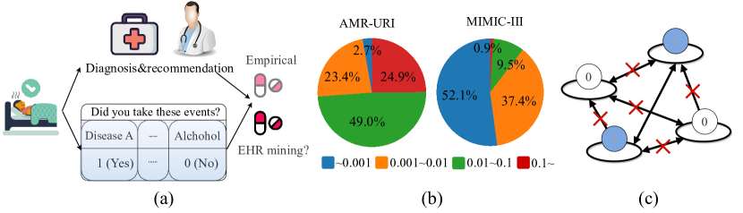
Figure 1: Ingredients of medication recommendation systems. Such systems automate diagnosis by digitalizing medical event outcomes (a). However, a pending challenge is that digital medical data often contains a significant amount of zero-like entries (b). For example, the proportion of non-zero values exceeding 10% is lower than 0.9% in MIMIC-III. In practice, those zero-like values pose a challenge to learning since they do not propagate learning signals (c).

Medication errors are one of the most serious medical errors that could threaten patients’ lives. Studies indicate that over 42% of these errors stem from physicians or doctors with insufficient experience or knowledge concerning specific drugs and diseases [28]. This challenge becomes even more pronounced with more new drugs and treatment guidelines. On the other hand, many patients are concurrently diagnosed with multiple diseases, complicating the decision-making process for doctors when determining more appropriate remedies for patients [33]. To this end, an automated medication recommendation system that can assist doctors in decision-making will be valuable to the medical community.

In the past decades, a vast amount of clinical data representing patient health status (e.g., medical reports, radiology images, and allergies) has been collected. This has remarkably increased digital information, known as electronic health records (EHR), available for patient-oriented decision-making. In this context, mining EHR data for medication recommendation has attracted growing research interests [33]. This paper investigates an EHR-based medication recommendation that leverages deep learning methods to pinpoint potential medication candidates for different ailments and patients, as illustrated in Fig. 1(a).

Successful methods typically rely on modeling outcomes of various medical events and diagnoses by observing longitudinal patient histories, i.e., tracking state variations across hospital visits [3, 38, 36, 33]. They often employ sequential neural networks, such as RNNs or Transformers. They construct a feature space centered around visits, wherein each visit is characterized by the current state of various medical events. Their objective is to discern long-range temporal dependencies that reflect the historical progression of diseases. These methods, however, suffer from a number of drawbacks. From a data viewpoint, different EHR databases adopt distinct visit recording methodologies [24]. For example, the AMR-URI database [14] employs a regular visit record, while visits in the MIMIC database [10] are patient-specific. Even within the same database, the time intervals between visits can differ greatly between patients. From a model perspective, a common obstacle is the "cold-start" issue, where medication recommendation systems struggle due to insufficient patient-specific historical data [37]. In practice, this issue becomes particularly pronounced when the system encounters newly onboarded patients, with scarce or even absent historical data (i.e., visits) about their medical backgrounds. While many researchers treat irregular time intervals as input variables [18, 15, 34] or apply the carry-forward imputation method [13], these approaches may introduce biases to temporal dependencies.

Some studies focus solely on a patient’s current diagnoses and medical event records, modeling event-event correlations for recommendation purposes without considering historical visits [38, 25]. However, a performance gap remains when compared to visit-based methods. A typical medical event has a binary value indicating its outcome: 1 for occurrence and 0 for non-occurrence, which leads to a sparsity issue in EHR data. The sparsity characterized by a high proportion of zero entries, can significantly impact the performance of recommendations (seen in Fig. 1(b)). From a modeling perspective, zero values provide no tangible information for deep learning models, preventing the activation of weight propagation. This often leads to a vanishing gradient problem and yields collapsed representations for medication recommendations (as shown in Fig. 1(c)). Previous studies employ secondary information, e.g., Drug-Drug Interaction Knowledge Graph (DDI-KG), to complement information to medical event features [33]. Yet, sparsity remains a persistent issue.

Therefore, this paper presents $\mathbb{BEHR}$NOULLI , a binary EHR data-oriented drug recommendation system. Our method is built upon a graph neural network (GNN) and solely utilizes the $\mathbb{EHR}$ binary medical events for recommendation. To tackle the binary data/sparsity, we take a statistical perspective that allows us to transform the 0, 1 values into continuous probabilistic representations, and estimate them from patient cohorts. Our statistical strategy has demonstrated substantial efficacy in modeling graphical structures and correlations within binary EHR data. Architecturally, diverse events are incorporated as node attributes within the GNN. When two events co-occur, we model their relationship as conditional Bernoulli probabilities to initialize the edge between them. This allows GNN to learn the correlations between events across different patients for medication recommendations. Our results demonstrate that our method outperforms several benchmarks, including the latest state-of-the-art (SOTA) visit-based methods. Specifically, our method shows an improvement on the MIMIC III dataset of approximately 4.8%, 6.7%, 6.3%, and 4% in terms of Jaccard, F1-score, PRAUC, and AUROC, respectively. $\mathbb{BEHR}$NOULLI is a simple and effective model that complements existing research in which the EHR data is often exploited in conjunction with secondary data but without transformations.

2 Related Works

- EHR-based Medication Recommendation. Historical Visit-based Methods: Many studies utilize deep learning to extract features from state variations across hospital visits in EHR data [5, 31, 30, 2, 25]. For example, DoctorAI [5] employs RNN to learn the dependencies of patients’ historical information and the doctor’s medication recommendations record for recommendation. MICRON [35] focuses on historical medication changes and medication combinations of the last visit. Some works introduce additional information to assist drug prediction, e.g., Drug-Drug Interaction (DDI) [36, 33].

Current Medical Event-based Methods: On the other hand, some works aim to analyze the patient’s current health status: recommendations are made based on the EHR records from each patient visit [38, 9, 23]. LEAP [38] encodes patient information in a one-hot encoding manner and then learns the relationship between patient features and drugs. SMR [9] incorporates additional information. It combines EHR data with an external medical knowledge graph to leverage external medical expertise in aiding the model decision-making process. MT-GIN [23] models event-event correlations in EHR data using a graph-based approach, with a focus on events that co-occur. This approach overlooks the information that 0 values in EHR binary data can potentially provide.

- Graph Modeling for Medication Recommendation. Recent research considers that event-event correlations can be well-captured by graph structures [5, 4, 25, 32, 22, 9, 27, 33, 23]. For instance, Gamenet [22] and Cognet [33] employ GNNs to discern correlations between different data types. They integrate DDI data into GNNs to understand the relationship graph between drugs, facilitating representation learning for medical events. GATE [25] proposes a GNN medication recommendation using events collected during a single visit. Further, COGNet [33] simultaneously models the EHR graph and the DDI graph, subsequently integrating them into a generative model. However, the above methods are designed on top of the binary value of medical events.

- Binary Data Representation. Mining binary data has been a longstanding challenge [7, 29]. One of the reasons is, that 0s and 1s can have entirely different meanings in various contexts or projects, making it difficult to interpret them uniformly [29]. Moreover, 0 values often provide nothing to the learning process, especially in deep learning models. In the EHR context, medGAN and POPCORN explicitly transform binary events in the EHR dataset into continuous probability values [6, 2]. However, these efforts primarily focus on modeling historical information or learning an overall distribution of the medical event outcomes. An effective medication recommendation method that directly represents binary events in EHR data remains challenging.

3 Problem Formulation

3.1 Recommendation System Based on EHR

EHR data consists of various medical events, such as multiple symptoms, recorded chronically from patients. Each data sample contains binary outcomes of these events. Let $\boldsymbol{x}\in\{0,1\}^{M}$ denote a patient EHR sample, where $M$ represents the total number of medical events, $1$ stands for the occurrence of the corresponding event, and $0$ for the absence. The EHR data is a matrix $\mathbf{X}\in\{0,1\}^{N\times M}$ composed by stacking $N$ patient vectors $\{\boldsymbol{x}\}_{1:N}$.

It is especially difficult to build effective recommendation systems using solely the EHR data, mainly due to the following reasons: (1) binary data poses a challenge to effective machine learning: while both 0 and 1 play an equally important role in identifying a proper recommendation, in practice 0 entries generally do not propagate learning signals; (2) medical events differ across platforms and as a result, two binary EHR matrices may share the same shape but completely different underlying meanings. Moreover, extracting such meanings and properly representing them, be it a series of same events recorded chronically, or different events that are highly correlated, is nontrivial.

Therefore, our goal is to effectively mine the complete information hidden in binary EHR data, based on which an effective, general-purpose recommendation system can be built. Formally, $\mathbb{BEHR}$NOULLI can be described by $F(\cdot):\{0,1\}^{M}\rightarrow\{0,1\}^{C}$, which accepts an EHR sample as input, and outputs $C$ binary indicators indicating whether or not recommend drug $i\in\{1,\dots,C\}$.

3.2 EHR as a Sample from the Population

To tackle the binary data, we take a statistical perspective in this paper. Several studies show many prevalent diseases and common medical conditions are often associated with commonalities among populations, such as shared living environments or behavioral habits [1]. In terms of epidemiology, temporal specificity and spatial specificity inevitably lead to a closer medical-relatedness among patients within the same sub-cohort compared to patients belonging to other sub-cohorts [26, 1, 19]. Inspired by this observation, we make two assumptions:

Assumption 1

the outcome of a medical event $E_{i}$ of the entire population is subject to a Bernoulli distribution.

Assumption 2

an EHR dataset is an i.i.d. sample from the population.

As such, an intuitive solution to the signal-stopping 0 entries is to represent them with the Bernoulli mean of the corresponding medical event $1-P(E_{i}=1)$. This Bernoulli mean can be empirically estimated from the EHR dataset which is assumed to be subject to the identical distribution as the population.

By mapping the 0-1 events to Bernoulli statistics, the equally important Yes/No outcomes have continuous representations. This can be important since the problem of data sparsity has been one of the most prominent obstacles to effectively mining the EHR data, as zero entries in practice do not propagate any learning signal. For instance, in deep learning models, a value of 0 cannot effectively activate the connection weights within a projection layer. Similarly, in graph-based models, zero values have no contribution to node attributes and message passing between nodes. As Bernoulli’s mean can take on any value between 0 and 1, this transformation also allows for more effective representations of the patient-event/event-event relationship. Quantifying such a relationship helps reflect the intrinsic connection between medical events, and contributes more to accurate medication recommendation than binary signals [16].

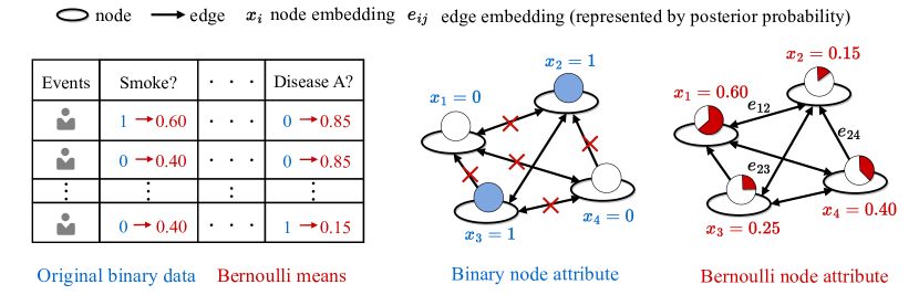
Figure 2: (Left) We transform the $\{0,1\}$ entries into Bernoulli means empirically estimated from the EHR samples, with the assumptions detailed in Section 4.1. (Middle) Graph learning directly on $\{0,1\}$ data can stall learning since zero entries prevent learning signals from propagating. (Right) Our proposed method learns from the Bernoulli transformed entries. Here, edges $e_{ij}$ are constructed from Bernoulli means, and nodes $x_{i}$ are constructed from conditional Bernoulli probabilities, see Algorithm 1.

4 Methodology

4.1 Patient-Event Graph Construction

We propose to learn by graph neural networks (GNNs) the inherent relationship between medical events within each patient sample as well as between an event and the patient population. A system overview has been shown in Fig. 2. Specifically, for each patient a graph $\mathcal{G}_{n}=(\mathcal{V}_{n},\mathcal{E}_{n})$ is constructed, where $\mathcal{V}_{n}$ denote the set of vertices, corresponding to the patient-event relationship; $\mathcal{E}_{n}$ the set of edges representing the event-event relationship. If we naïvely initialized the $\mathcal{V}_{n},\mathcal{E}_{n}$ by the elements of $\mathbf{X}$, the zero entries may cause significant loss of information of the non-occurrence of events since zero values typically stall the propagation of learning signals. Therefore, we propose to initialize them in the following approach.

Patient-to-patient correlation embedding. By assumption (i) in Section 3.2, the occurrence of an event is subject to a Bernoulli distribution $P(E_{j}=k)=\rho^{k}(1-\rho)^{k}$, where $k\in\{0,1\}$, and $\rho$ denotes the mean of the distribution. By assumption (ii), the event in the EHR data sample is subject to the same distribution $P(\mathbf{X}_{\cdot j}=k)=\rho^{k}(1-\rho)^{k}$, where we denote the $\mathbf{X}_{\cdot j}$ denote the event $E_{j}$ for all patient samples. Therefore, we propose to initialize the vertices by the Bernoulli mean $\rho$. While this quantity is not known, we can replace it with a sample estimate:

$$\tilde{\rho}:=\tilde{P}(X_{\cdot j}=1)=\frac{\sum_{i=1}^{N}\mathbf{X}_{ij}}{N},\,\,\tilde{P}(X_{\cdot j}=0)=1-\tilde{\rho}.$$

Event-to-event correlation embedding. Following this idea, we propose to initialize the edges representing the event-to-event relationship by conditional Bernoulli probability. Intuitively, an edge from event $j$ to event $i$ encodes some information conditional on the observation of $i$ [4, 17]. From this consideration, we initialize the edge $e_{ij}$ from event $E_{j}$ to event $E_{i}$ with:

$$e_{ij}:=P(E_{i}=1|E_{j}=1)=\frac{{P}(E_{i}=1\text{ and }E_{j}=1)}{{P}(E_{j}=1)}.$$

Again, while the exact distribution is not known, we can replace it with sample estimate: the conditional probability is instead estimated by

$$\frac{P(\mathbf{X}_{\cdot i}=1\text{ and }\mathbf{X}_{\cdot j}=1)}{P(\mathbf{X}_{\cdot j}=1)}=\frac{\#\{\text{patients with positive event }i\text{ and }j\}}{\#\{\text{patients with positive event }j\}}.$$

It is worth noting that the proposed initialization can be seen as a transformation from binary data to continuous values. In the experiments, we shall also compare against other transformation methods.

Algorithm 1 Pseudocode of patient-event graph construction.

⬇

def generate_patient_graph(EHR_Matrix):

# EHR_Matrix: Rows represent patients and columns represent medical events

# Calculate proportions of each event based on all patients

event_proportions = mean(EHR_Matrix, axis=0)

# Calculate posterior probabilities between each pair of events, for the pair of event i and event j:

posterior probability(event i, event j) = $\frac{{\text{Proportion}}(\text{event i}=1\text{ and }\text{event j}=1)}{{\text{Proportion}}(\text{event j}=1)}$ = $\frac{\text{number of}(\text{event i}==1\;\text{and}\;\text{event j}==1)}{\text{number of all patients}}/\frac{\text{number of}(\text{event j}==1)}{\text{number of all patients}}$

For each patient, generate a graph:

# Determine node embeddings based on the patient’s medical event data

node_embeddings = event_proportion if input value == 1

node_embeddings = 1-event_proportion if input value == 0

# Determine edge weights based on the posterior probabilities between each pair of events

edge_weights of (edge between node i and node j) =

posterior probability of (event i and event j)

4.2 Patient-to-Event Graph Learning

In Section 4.1, we mapped each patient sample $\mathbf{X}_{i\cdot}$ to a graph $\mathcal{G}_{i}=(\mathcal{V}_{i},\mathcal{E}_{i})$, with empirical Bernoulli mean initialization. This transformation converts the original drug recommendation binary classification problem into a graph classification problem. Specifically, we first map the EHR data into a set of vertices and edges $\{0,1\}^{M}\stackrel{{\scriptstyle\text{B.I.}}}{{\rightarrow}}\mathcal{V}_{i},\mathcal{E}_{i}\in[0,1]^{M}$, where B.I. denote Bernoulli Initialization. A graph learning function is then applied to output final drug recommendations $F(\cdot):\mathcal{V}_{i},\mathcal{E}_{i}\rightarrow\{0,1\}^{C}$. We employ EGraphSage [12] as our $F$. We obtain the node and edge embeddings $h_{\nu},h_{e}$ by passing them through a simple MLP. Note that the first layer of the MLP has an interpretation of nonlinearly transforming the Bernoulli statistics residing on the nodes and edges we initialized. The graph learning process aims to discern correlations between events through message aggregation and adjust the event (node) attribute for each patient by updating the node features.

Now for each edge $e_{ij}$ from node $i$ to node $j$, compute the message $m_{j}$ using:

$$m_{j}=\text{relu}\left(\mathbf{W}_{m}\times\left(h_{\nu_{j}}\oplus h_{e_{ij}}\right)\right)$$

Here, $\oplus$ represents concatenation, $\mathbf{W}_{m}$ is a learnable weight matrix for message passing, and relu is a non-linear activation function.

Message aggregation: After obtaining the message, we aggregate messages $m_{j}$ across edges for each node:

$$\text{AGGREGATE}_{i}=\frac{1}{|\mathcal{N}(i)|}\sum_{j\in\mathcal{N}(i)}m_{j}$$

Where $\mathcal{N}(i)$ represents the set of neighbors of the node $i$.

Update node features: We update and normalize the node feature $h_{\nu_{i}}$ for each node $\nu_{i}$ using:

$$h_{\nu_{i}}=\text{activation}\left(\mathbf{W}_{u}\times\left(h_{\nu_{i}}\oplus\text{AGGREGATE}_{i}\right)\right),\,\,h_{\nu_{i}}^{\prime}=\frac{h_{\nu_{i}}^{\prime}}{\|h_{\nu_{i}}^{\prime}\|_{2}}$$

Where $h_{\nu_{i}}^{\prime}$ is the updated feature of node $i$, and $\mathbf{W}_{u}$ is learnable weight matrix for updating, $\|.\|_{2}$ denotes the L2 norm.

4.3 Medication Recommendation

After $K$ iterations, the last layer’s updated node feature $(h^{\prime}_{\nu},\forall{\nu\in\mathcal{V}})$ serves as the output of our graph embedding learning part. After obtaining the node embeddings $h^{\prime}_{\nu}$ for each graph, we concatenate these embeddings to form a single feature vector for each graph. This is represented as: $\mathbf{z}_{\mathcal{G}_{i}}=\oplus_{(\nu\in\mathcal{V})}h^{\prime}_{\nu},$ Where $\mathbf{z}_{\mathcal{G}_{i}}$ is the concatenated feature vector for graph $\mathcal{G}_{i}$ and $\oplus$ denotes the concatenation operation over all nodes (i.e., medical events).

The concatenated feature vectors $\mathbf{z}_{\mathcal{G}_{i}}$ for each graph are then passed through a linear projection for classification. The linear layer has $Y$ independent output dimensions, each corresponding to a binary classification task. Formally, for each output dimension $y$, the operation is:

$$\mathbf{o}_{y}=\text{sigmoid}\left(\text{Linear}\left(\mathbf{z}_{\mathcal{G}_{i}}\right)\right)$$

$$\mathbf{r}_{y}=\begin{cases}1&\text{if }\mathbf{o}_{y}>0.5\\ 0&\text{otherwise}\end{cases}$$

Upon processing each graph’s feature vector $\mathbf{z}_{\mathcal{G}_{i}}$, the system yields $Y$ independent outputs. Each of these outputs specifically corresponds to the recommendation decision for a drug. The decision is binary: either the medication is recommended (represented by a value of 1) or not (represented by 0).

5 Experiments

5.1 Databases

We evaluated the performance of $\mathbb{BEHR}$NOULLI on two large-scale datasets: the Medical Information Mart for Intensive Care (MIMIC-III) dataset and the Antimicrobial Resistance in Urinary Tract Infections (AMR-UTI). Both databases have been extensively utilized for benchmarking and are available on PhysioNet.

- MIMIC-III represents a vast repository of de-identified health data from intensive care unit (ICU) patients at the Beth Israel Deaconess Medical Center in Boston, Massachusetts [10]. It contains a total of 46520 patients from 2001 to 2012. In this database, the patient data we used was sourced from three sub-datasets, ’ADMISSIONS’, ’DIAGNOSES_ICD’, and ’PROCEDURES_ICD’.

Table 1: Datasets description

Dataset	MIMIC	AMR-URI
#Medical event	3388	692
#Drug candidate	131	4
Sparsity of features	0.9946	0.9309
Sparsity of label	0.8534	0.5423

- AMR-UTI dataset contains EHR information collected from 51878 patients from 2007 to 2016, with urinary tract infections (UTI) treated at Massachusetts General Hospital and Brigham & Women’s Hospital in Boston, MA, USA [14]. Each patient in this dataset provided a series of binary indicators for whether the patient was undergoing a specific medical event. There are four common antibiotics (medication labels): nitrofurantoin (NIT), TMP-SMX (SXT), ciprofloxacin (CIP) or levofloxacin (LVX).

Table 1 shows some statistics on two databases. The sparsity of a matrix can be calculated using the formula: $Sparsity=1-\frac{\text{Number of Non-Zero Elements}}{\text{Total Number of Elements}}$. The high degree of sparsity observed in the feature dimensions for both the MIMIC-III and AMR-URI datasets may constitute a significant impediment to the efficacy of the machine learning models.

Data preprocessing. For MIMIC-III, we referred to the data processing released by [36, 33] for fairness. Only the patients with at least 2 visits are incorporated. The medications were selected and retained based on their frequency of occurrence (the top 300). For AMR-URI, we first excluded the basic demographic information including age and ethnicity. The observations that do not have any health event or drug recommendation were removed. For each observation, a feature was constructed from its EHR as a binary indicator for whether the patient is undergoing a particular medical event within a specified time window. After the above preprocessing, we divided both datasets into training, validation and testing by the ratio of 3/5, 1/5, and 1/5. More detailed description of data processing can be found in Appendix 0.B.

5.2 Baselines

We selected three categories of methods as the baseline: statistics-based, RNN-based, and GNN-based models.

- Statistics work. we select the standard Logistic Regression (LR) and Ensemble Classifier Chain (ECC)  [20] as the baseline.

- RNN-based works. RETAIN  [3] incorporates two-level attention with gating mechanisms to detect significant clinical variables. LEAP  [38] is an LSTM-based generation model, leveraging a reinforcement learning module to prevent generating unfavorable drug combinations. DMNC  [11] proposes a new memory-augmented neural network model to improve the patient encoder.

- GNN-based works., GAMENet  [22] integrates the knowledge graph of Drug-Drug Interaction (DDI) by a graph convolutional networks. Further, SafeDrug  [36] combines the drug molecular graph with the DDI graph to predict the safe medication combination. COGNet  [33] retrieves patients’ historical diagnoses and medication recommendations and mines their relationship with current diagnoses via a Conditional Generation Net. In addition to modeling the graph of DDI, MI-GIN [23] directly modeled the EHR data itself in a graph approach. A graph Isomorphism neural network based on multi-task learning is used for medication recommendation.

Moreover, we used the Jaccard Similarity Score (Jaccard), Average F1 (F1), AUROC (Area Under the ROC Curve), Precision-Recall AUC (Area Under the Precision-Recall Curve), and average predicted number of drugs (#Drug) as our evaluation metrics. Each evaluation result was an average of all patients. We further utilized Precision and Recall to evalute the medication recommendation. The parameter settings can be found in Appendix 0.C.

5.3 Ablation Study

We conducted several ablations for evaluating different modeling methods of node/edge attributes. The main contributions of $\mathbb{BEHR}$NOULLI lie in the transformation of binary medical events into continuous values (Bernoulli means). We selected two classic methods for encoding categorical features into continuous values: Log Likelihood Ratio (LLR) and Target Encoding (TE) [21]. The detailed descriptions of these two methods can be found in Appendix 0.D. We further compared against random initialization of nodes and edges for ablation evaluation, and assessed $\mathbb{BEHR}$NOULLI without node or edge construction. The details of ablation study are as follows:

• $\mathbb{BEHR}$NOULLI : BM (Bernoulli means)$w/$ Post (posterior): Our proposal.

• BM $w/o$ Post: we maintained the node embedding but replace the posterior edge embedding with the simple co-occurrence between medical events.

• LLR $w/$ Post: we replaced the Bernoulli means node embedding with LLR.

• LLR $w/o$ Post: we used LLR as the simple co-occurrence embedding.

• TE $w$ Post: we replaced the Bernoulli means node embedding with TE.

• TE $w/o$ Post: we used TE as the simple co-occurrence embedding.

• BM $w/$ RE: we replaced the posterior edge embedding with random edge (RE) initialization.

• RN $w/$ Post: we replaced the Bernoulli means node embedding with random node (RN) initialization.

• RN $w/$ RE: Both Bernoulli means and posterior embedding were replaced with random initialization.

Moreover, we conducted model ablation to evaluate the event-event graphical correlation modeling compared to different model strategy of simple linear projection (MLP), LSTM and Transformer. All of the implementation details of the baseline comparison and ablation study can be found in Appendix 0.E.

Table 2: Performance Comparison on MIMIC-III and AMR-UTI. Best results are highlighted in bold fonts, second-best results are underscored. The results (-) denote models that do not converge, regardless of any model fine-tuning effort.

Dataset	MIMIC							AMR-UTI
Baseline	Methods	Jaccard	F1	PRAUC	AUROC	#Drug		Jaccard	F1	PRAUC	AUROC	#Drug
LR	Stat	0.4865	0.6434	0.7509	0.9180	16.1773		0.3803	0.5018	0.4624	0.5057	1.4869
ECC	Stat	0.4996	0.6569	0.6844	0.9098	18.0722		0.6080	0.6665	0.6914	0.7273	1.7040
RETAIN	RNN	0.4877	0.6481	0.7556	0.9234	20.4051		-	-	-	-	-
LEAP	RNN	0.4521	0.6138	0.6549	0.8927	18.7138		-	-	-	-	-
DMNC	RNN	0.4864	0.6529	0.7580	0.9157	20.0000		-	-	-	-	-
SafeDrug	RNN	0.5213	0.6768	0.7647	0.9219	19.9178		-	-	-	-	-
GAMENet	Graph	0.5067	0.6626	0.7631	0.9237	27.2145		0.6024	0.6433	0.6913	0.7174	1.7106
COGNet	Graph	0.5336	0.6869	0.7739	0.9218	28.0903		0.5287	0.6359	0.5717	0.6281	1.6331
MT-GIN	Graph	0.5401	0.7781	0.7812	0.9115	16.1233		0.5137	0.6124	0.6779	0.6428	1.4991
Proposal	Graph	0.5887	0.8459	0.8442	0.9632	15.7129		0.6116	0.6753	0.7071	0.7401	1.5973

6 Results

6.1 Comparison Against Baselines

Main Results. Table 2 shows the main results for medication recommendation on two databases. Overall, our proposed $\mathbb{BEHR}$NOULLI outperforms all baselines on all metrics (Jaccard, F1, PRAUC, and AUROC). Given that most results were directly collected from the original study [33], $\mathbb{BEHR}$NOULLI demonstrates superior performance for the MIMIC-III dataset. It outperforms other approaches, even those that incorporate additional data types, secondary information, and visit modeling for medication recommendations. Some statistical models, such as LR and ECC, outperform early RNN-based baselines LEAP, DMNC, and RETAIN, demonstrating ECC achieves the best results in Jaccard and F1. The difficulties of RNN-based models lie in handling missing historical data, inconsistent data formats in historical records, and the inability to handle situations where no historical data is available. Similar results have been shown in AMR-UTI; given that six visit datasets could serve as the RNN’s timesteps, it often vanishes gradients within various model fine-tunings. Graph-based methods tend to converge well and result in better performances compared to RNN baselines. This shows the effectiveness of modeling event-event correlations and structure information. While $\mathbb{BEHR}$NOULLI is solely based on binary medical events, further integrating this binary data modeling with external EHR information, like DDI, could enhance recommendation performance.

Visit-Included Results. The results presented in Table 2 exclude information derived from patient visits. To provide a more comprehensive assessment incorporating visit data, we present an average recommendation performance across all patient visits in Table 3. Specifically, some of the baseline methods rely on sequential learning. In these approaches, during each visit, every medication is allocated a recommendation probability upon its generation.

Table 3: Comparison when visiting information is included on MIMIC-III. Though $\mathbb{BEHR}$NOULLI is not explicitly designed to incorporate secondary information, it outperforms existing visiting-aware methods when evaluated on the same benchmarks. Bold: best; underscored: second-best.

Model	Jaccard	F1	PRAUC	AUROC	#Drug
LR	0.4844	0.6483	0.7492	0.9029	16.1221
ECC	0.5003	0.6590	0.6802	0.9214	18.4127
RETAIN	0.4876	0.6484	0.7594	0.9225	19.8297
LEAP	0.4487	0.6119	0.6480	0.8927	19.1095
DMNC	0.4834	0.6492	0.7569	0.9237	20.1087
GAMENet	0.5084	0.6648	0.7670	0.9235	26.1983
SafeDrug	0.5276	0.6692	0.7649	0.9218	19.8847
COGNet	0.5127	0.6850	0.7739	0.9266	27.3277
MT-GIN	0.5273	0.7527	0.7499	0.9188	15.1233
Proposed	0.5902	0.8465	0.8448	0.9635	15.6944

We first average their performance over multiple visits for each patient and then further average these results across all patients. In this context, $\mathbb{BEHR}$NOULLI shows an effective and robust performance and outperforms all baselines.

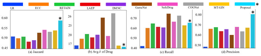
Figure 3: Comparison between the proposed method and baselines using four widely adopted metrics (Jaccard, Avg of Drug, Recall, Precision). The proposed method outperforms all baselines on all evaluation benchmarks.

Medication Recommendation Analysis. Fig. 3 provides an extensive comparison of Precision and Recall metrics for medication recommendation across all baselines and $\mathbb{BEHR}$NOULLI. It’s essential to evaluate drug recommendation systems from multiple dimensions. Hence, we utilize several evaluation metrics to ensure a comprehensive comparison of our approach against existing methods. One prevalent issue is the False Positive (FP) problem, where the recommendation system suggests an unsuitable or unnecessary drug to a patient. This results in a relatively high recall but a low precision due to incorrect recommendations. On the other hand, the False Negative (FN) issue happens when the recommendation system fails to suggest a drug that would have been beneficial for the patient. This results in low recall because it fails to capture a relevant recommendation. However, precision can still be high for recommendations. In Fig. 3, the ground truth of the average number of recommendations is 19.2268 in the MIMIC-III dataset $\mathbb{BEHR}$NOULLI has shown a similar performance with 15.7129 average recommendations. This indicates $\mathbb{BEHR}$NOULLI tends to recommend a precise (high Jaccard and Precision scores) but fewer number of drugs out of 131 while still achieving competitive recall rates.

Table 4: Ablation study on node and edge embeddings. We compare various embedding methods for node/edge attributes to validate the contributions of the proposed embedding approach. Bold: best; underscored: second-best.

Dataset	MIMIC						AMR-UTI
Metrics	Jaccard	F1	PRAUC	AUROC	#Drug		Jaccard	F1	PRAUC	AUROC	#Drug
BM $w/o$ Post	0.5482	0.8275	0.151	0.9542	15.1754		0.6109	0.6750	0.7066	0.7378	1.5966
LLR $w/$ Post	0.5398	0.8234	0.8104	0.9527	14.8922		0.6091	0.6748	0.7052	0.7322	1.5990
LLR $w/o$ Post	0.4367	0.7717	0.7265	0.242	12.7554		0.6089	0.6732	0.7048	0.7318	1.5964
TE $w/$ Post	0.3904	0.7475	0.6947	0.9116	11.7528		0.0186	0.3580	0.4961	0.5387	0.0172
TE $w/o$ Post	0.3904	0.7475	0.6947	0.9116	11.7528		0.0001	0.3507	0.4595	0.5000	0.0001
BM $w/$ RE	0.5692	0.8261	0.8230	0.9428	15.8093		0.6019	0.6579	0.6881	0.7218	1.6220
RN $w/$ Post	0.2941	0.6674	0.4902	0.8174	24.8895		0.5974	0.3554	0.4685	0.4776	2.9293
RN $w/$ RE	0.2932	0.6640	0.4899	0.8075	24.8788		0.5963	0.3530	0.4601	0.4744	2.9275
MLP backbone	0.3926	0.7484	0.6871	0.8948	12.0562		0.5667	0.6685	0.6945	0.7137	1.4853
LSTM backbone	0.3868	0.7454	0.6940	0.9102	11.4403		0.5352	0.6491	0.6810	0.7217	1.3640
Transformer backbone	0.3907	0.7475	0.6867	0.8996	11.9148		0.5100	0.3512	0.4662	0.5088	1.3470
Ours (BM $w/$ Post)	0.5887	0.8459	0.8442	0.9632	15.7129		0.6116	0.6753	0.7071	0.7401	1.5973

6.2 Ablation Study

For ablations on node and edge embeddings, Table 4 shows that among various embedding strategies on both datasets, combining our Bernoulli mean node embedding with posterior probability edge embedding achieves the best results. If we compare the contributions of node (Bernoulli mean) and edge (posterior probability) embeddings to the graph-based drug recommendation results, we find that node embedding has a relatively more substantial impact. The random node destroys the recommendation performance even when considering posterior probabilities, resulting in a significantly low Jaccard score of 0.29. However, using the Bernoulli mean for edge embedding initialization yields a much better performance, with a Jaccard score of 0.5692. This could be because node embedding directly represents the original EHR data, while edges are inferred based on the original data to model the relationship between different events. On the other hand, the purpose of using GNN is to capture event-event correlations. Therefore, edge embeddings merely aid in GNN computations. The results show that even without initializing edge embeddings with posterior probabilities, GNN can still capture event-event correlations, though with a performance decrease. For model ablation, GNN outperforms all baselines (i.e., MLP, LSTM, and Transformer) on two datasets.

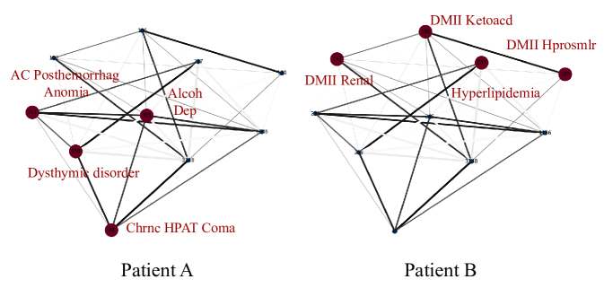
Figure 4: Visualization of features learned by $\mathbb{BEHR}$NOULLI . Each node denotes an event and edges represent event-event correlations. A thicker edge shows a stronger event-event association, and nodes with higher values are highlighted.

6.3 Visualization of Recommendations

Fig. 4 shows representations learned by GNN for two different patients, on a subset of EHR medical events. GNN produces distinct feature values for different nodes, for visualization and better understanding, we processed the node feature values using the TOP-K approach, highlighting the top K nodes with the highest feature values. It can be observed that GNN has learned completely different representations for different patients and has emphasized different features on various nodes. For instance, the "Hyperlipidemia" node, which is highlighted in Patient B’s data, receives a lower weight in Patient A’s data. This indicates that this event is more critical in Patient B’s data compared to Patient A. Moreover, GNN has learned certain connections between important features for each patient. This result highlights how the same event can exhibit entirely different levels of importance across different patients’ data. For example, in Patient B’s data, three identical series (MDII) of medical events are simultaneously highlighted. Through this simple analysis, we confirmed that GNN learned different representations for different patients, providing valuable information for downstream tasks. More results can be found in Appendix 0.F.

7 Conclusion

In this paper we proposed the first binary EHR data oriented drug recommendation system, by transforming the problematic 0,1 binary event outcomes to continuous Bernoulli means. We took a statistical perspective by viewing the EHR data as a sample from the greater population. In this manner, we modeled the nodes and edges of GNN using the Bernoulli distribution. Extensive results showed that our method attained the SOTA and outperformed all baselines by a large margin; and some of the baselines learned from significantly more information resources such as the visiting data and drug-drug interactions, while ours learned solely from the binary data. Ablation studies verified the importance of the Bernoulli transformation of EHR binary data. By replacing only edges (conditional probability) and keeping nodes (Bernoulli mean) fixed, we observed largely reduced improvement compared to the proposed method. On the other hand, assigning Bernoulli means to the nodes resulted in significantly better performance even with random edge values. These findings confirm that $\mathbb{BEHR}$NOULLI is a simple and effective model, highlighting its potential for integration into more sophisticated systems.

Appendix 0.A Source Code

The code link is: https://github.com/chenzRG/BEHRMecom

Appendix 0.B Preprocessing

0.B.1 Data Profile

Data Sources: The data is sourced from the MIMIC dataset, a publicly available dataset developed by the MIT Lab for Computational Physiology, comprising de-identified health data from over 40,000 critical care patients. The primary datasets in focus for preprocessing include:

• Medications (‘PRESCRIPTIONS.csv‘): Contains records of medications prescribed to patients during their ICU stays.

• Diagnoses (‘DIAGNOSES ICD.csv‘): Lists diagnosis codes associated with each hospital admission.

• Procedures (‘PROCEDURES ICD.csv‘): Catalog procedures that patients underwent during their hospital visits.

Data Structure: The data is structured in tabular format. Each table contains unique identifiers for patients (‘SUBJECT ID‘), their specific hospital admissions (‘HADM ID‘), and other clinical details pertinent to the dataset in question.

0.B.2 Medication Data Preprocessing

Data Loading and Initial Processing:

• Load the Data: The medication data from ‘PRESCRIPTIONS.csv‘ is loaded into a data frame.

• Filter Columns: Only essential columns, namely ‘pid‘, ‘adm id‘, ‘date‘, and ‘NDC‘, are retained.

• Data Cleaning: Entries with ’NDC’ equal to ’0’ are dropped, and any missing values are filled using the forward-fill method.

• Data Transformation: The ‘STARTDATE‘ field is converted to a DateTime format for easier manipulation and analysis.

• Sorting and Deduplication: The dataset is sorted by multiple columns, including ‘SUBJECT ID‘, ‘HADM ID‘, and ‘STARTDATE‘, and any duplicate entries are removed.

Medication Code Mapping:

• Mapping NDC to RXCUI: The ‘NDC‘ codes are mapped to the ‘RXCUI‘ identifiers using a separate mapping file.

• Mapping RXCUI to ATC4: The ‘RXCUI‘ identifiers are further mapped to the ‘ATC4‘ codes using another mapping file. The ATC classification system is crucial for grouping drugs into different classes based on their therapeutic use.

0.B.3 Diagnosis Data Preprocessing

The diagnosis data from ‘DIAGNOSES ICD.csv‘ is processed using the ‘diag process‘ function, which involves:

• Load the Data: Diagnosis data is loaded into a data frame.

• Filter Relevant Columns: Only essential columns, which might include diagnosis codes and patient identifiers, are retained.

• Handle Missing or Erroneous Entries: Any missing values or errors in the dataset are addressed, ensuring data integrity.

• Sorting and Deduplication: The dataset is sorted based on relevant columns, and duplicate entries are removed to ensure each record is unique.

0.B.4 Procedure Data Preprocessing

Similar to the diagnosis data, the procedure data from ‘PROCEDURES ICD.csv‘:

• Load the Data: Procedure data is loaded into a DataFrame.

• Filter and Clean: Only relevant columns are retained, and any erroneous or missing entries are addressed.

• Sorting and Deduplication: The data is organized by relevant columns, and any duplicate records are removed.

0.B.5 Data Integration

Combining Process: The datasets, once cleaned and preprocessed, need to be integrated for comprehensive analysis:

• Data Merging: The medication, diagnosis, and procedure data are merged based on common identifiers like ‘SUBJECT ID‘ and ‘HADM ID‘.

• Final Cleaning: Any discrepancies resulting from the merge, such as missing values or duplicates, are addressed.

Appendix 0.C Model Parameters

GNN Model (EGraphSage) The Graph Neural Network model is implemented using the EGraphSage class. The configuration parameters for the model are in the Table 5

Table 5: Datasets description

Dataset	GNN	MLP
Input Dimension	1	#nodes
Hidden Layer Dimension	128	64
Output Dimension	1	1
Edge Channels	1	NaN
Activation Function	ReLU	ReLU
Aggregation Method	Mean	NaN

Appendix 0.D Metrics

Target encoding is a popular technique in machine learning for encoding categorical features, where each category is replaced with its corresponding mean target value. This can be mathematically expressed as:

$$\text{Target Encoding}(c)=\frac{\sum_{i=1}^{N}y_{i}\cdot\delta(c,c_{i})}{\sum_{i=1}^{N}\delta(c,c_{i})}$$

where $c$ represents the category to be encoded, $y_{i}$ is the target value for the $i$-th sample, $c_{i}$ is the category of the $i$-th sample, and $\delta(c,c_{i})$ is the Kronecker delta function that equals 1 when $c$ equals $c_{i}$ and 0 otherwise.

Log Likelihood Ratio (LLR): The likelihood ratio is defined as the ratio of two key values: The maximum value of the likelihood function is calculated within the subspace defined by the hypothesis. And the maximum value of the likelihood function, calculated across the entire parameter space [8].

To compute the score, let $k_{11}$ be the number of times the events occurred together, let $k_{12}$ and $k_{21}$ be the number of times each has occurred without the other, and $k_{22}$ be the number of times something has been observed that was neither of these events. The LLR score is given as the following:

$$LLR=2\sum(k)\left(H(k)-H(\text{rowSums}(k))-H(\text{colSums}(k))\right)$$

where $H$ is Shannon’s entropy, computed as the sum of:

$$H=\frac{k_{ij}}{\sum(k)}\log\left(\frac{k_{ij}}{\sum(k)}\right).$$

In our case, when calculating the similarity measure between a medical event and the recommendation of a specific drug, we calculated the LLR value by the counts that co-occurred between them. The average LLR for each medical event with all recommended drugs was calculated as the properties of the medical event node [8].

Appendix 0.E Implementation Details

The models mentioned were implemented by PyTorch 2.0.1 based on Python 3.8.8, All experiments are conducted on an Intel Core i9-10980XE machine with 125G RAM and an NVIDIA GeForce RTX 3090. For the experiments on both datasets, we chose the optimal hyperparameters based on the validation set. Models were trained on Adam optimizer with learning rate $1\times 10^{-4}$ for 200 epochs. The random seed was fixed as 0 for PyTorch to ensure the reproducibility of the models.

For a fair comparison, we employed bootstrapping sampling instead of cross-validation in the testing phase. Specifically, in each evaluation round, we randomly sampled $80\%$ of the data from the test set. We repeated this process 10 times to obtain the final results. These results from 10 rounds were then used to calculate both the mean and standard deviation. The means are reported in Table 2. The standard deviations are all under 0.05.

Appendix 0.F More Results

Figure 5 shows another visualization of features learned by GNN from patients’ EHR data. This time we peak another set of medical events on other two different patients.

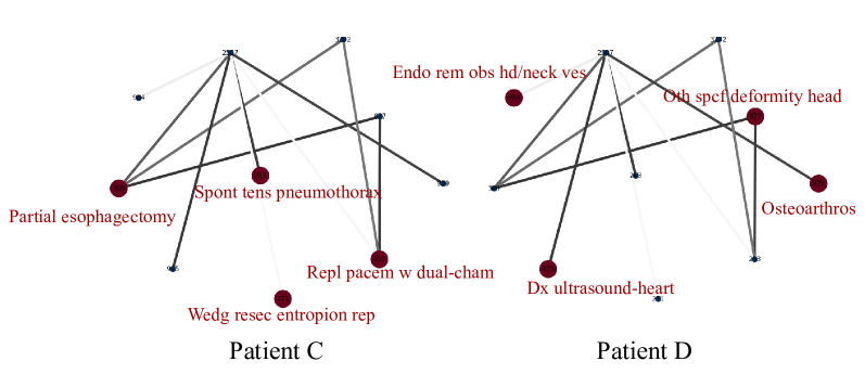
Figure 5: Another visualization of features learned by GNN from patients’ EHR data. Each node represents a different event, and edges represent relationships between events. Thicker edges indicate a stronger association between two events. Nodes with higher feature values have been highlighted.

References

- [1] Bache, R., et al.: An adaptable architecture for patient cohort identification from diverse data sources. JAMIA pp. 327–333 (2013)
- [2] Bhave, S., Perotte, A.: Point processes for competing observations with recurrent networks (popcorn): A generative model of ehr data. In: ML4H. pp. 770–789 (2021)
- [3] Choi, E., et al.: RETAIN: an interpretable predictive model for healthcare using reverse time attention mechanism. In: NIPS. pp. 3504–3512 (2016)
- [4] Choi, E., et al.: Learning the graphical structure of electronic health records with graph convolutional transformer. In: AAAI. pp. 606–613 (2020)
- [5] Choi, E., et al.: Doctor ai: Predicting clinical events via recurrent neural networks. In: ML4H. pp. 301–318 (2016)
- [6] Choi, E., et al.: Generating multi-label discrete patient records using generative adversarial networks. In: ML4H. pp. 286–305 (2017)
- [7] D, C., Stepniewska, K.: Some practical issues in binary data analysis. Statistics in medicine pp. 17–18 (1999)
- [8] Dunning, T.: Accurate methods for the statistics of surprise and coincidence. Computational linguistics pp. 61–74 (1994)
- [9] Gong, F., et al.: SMR: medical knowledge graph embedding for safe medicine recommendation. Big Data Res (2021)
- [10] Johnson, A.E.W., et al.: Mimic-iii, a freely accessible critical care database. Scientific Data (2016)
- [11] Le, H., et al.: Dual memory neural computer for asynchronous two-view sequential learning. In: KDD. pp. 1637–1645 (2018)
- [12] Lo, W.W., et al.: E-graphsage: A graph neural network based intrusion detection system for iot. In: NOMS. pp. 1–9 (2022)
- [13] Luo, Y.: Evaluating the state of the art in missing data imputation for clinical data. Briefings in Bioinformatics (2022)
- [14] Michael, O., et al.: Amr-uti: Antimicrobial resistance in urinary tract infections (version 1.0.0). PhysioNet (2020)
- [15] Miotto, R., Li, L., Kidd, B.A., Dudley, J.T.: Deep patient: an unsupervised representation to predict the future of patients from the electronic health records. Scientific reports pp. 1–10 (2016)
- [16] M.M., Y., et al.: Pharmacological options for smoking cessation in heavy-drinking smokers. CNS Drugs p. 833–845 (2015)
- [17] Murphy, K.P.: Probabilistic machine learning: Advanced topics. MIT press (2023)
- [18] Nguyen, P., et al.: Deepr: a convolutional net for medical records. IEEE JBHI pp. 22–30 (2016)
- [19] Poulakis, K., et al.: Multi-cohort and longitudinal bayesian clustering study of stage and subtype in alzheimer’s disease. Nature com (2022)
- [20] Read, J., et al.: Classifier chains for multi-label classification. In: ECML-PKDD. pp. 254–269 (2009)
- [21] Rodríguez, P., et al.: Beyond one-hot encoding: Lower dimensional target embedding. Image and Vision Computing pp. 21–31 (2018)
- [22] Shang, J., et al.: Gamenet: Graph augmented memory networks for recommending medication combination. In: AAAI. pp. 1126–1133 (2019)
- [23] Shu, H., et al.: Drugs resistance analysis from scarce health records via multi-task graph representation. In: ADMA. p. 103–117 (2023)
- [24] Singh, A., et al.: Incorporating temporal ehr data in predictive models for risk stratification of renal function deterioration. JBI pp. 220–228 (2015)
- [25] Su, C., Gao, S., Li, S.: Gate: graph-attention augmented temporal neural network for medication recommendation. IEEE Access pp. 125447–125458 (2020)
- [26] Sun, J., et al.: Supervised patient similarity measure of heterogeneous patient records. Acm SIGKDD Explorations Newsletter pp. 16–24 (2012)
- [27] Tan, Y., et al.: 4sdrug: Symptom-based set-to-set small and safe drug recommendation. In: KDD. pp. 3970–3980 (2022)
- [28] Tran, T.N.T., et al.: Recommender systems in the healthcare domain: state-of-the-art and research issues. Journal of Intelligent Information Systems pp. 1–31 (2021)
- [29] Verstrepen, K., et al.: Collaborative filtering for binary, positiveonly data. SIGKDD Explor. Newsl. p. 1–21 (2017)
- [30] W, S., et al.: Order-free medicine combination prediction with graph convolutional reinforcement learning. In: CIKM. pp. 1623–1632 (2019)
- [31] Wang, L., et al.: Supervised reinforcement learning with recurrent neural network for dynamic treatment recommendation. In: KDD. pp. 2447–2456 (2018)
- [32] Wharrie, S., Yang, Z., Ganna, A., Kaski, S.: Characterizing personalized effects of family information on disease risk using graph representation learning (2023)
- [33] Wu, R., Qiu, Z., Jiang, J., Qi, G., , Wu, X.: Conditional generation net for medication recommendation. In: WWW. p. 935–945 (2022)
- [34] Xiang, Y., et al.: Time-sensitive clinical concept embeddings learned from large electronic health records. BMC MIDM pp. 139–148 (2019)
- [35] Yang, C., et al.: Change matters: Medication change prediction with recurrent residual networks. In: IJCAI. pp. 3728–3734 (2021)
- [36] Yang, C., et al.: Safedrug: Dual molecular graph encoders for safe drug recommendations. In: IJCAI (2021)
- [37] Ye, Q., et al.: A unified drug–target interaction prediction framework based on knowledge graph and recommendation system. Nature communications pp. 67–75 (2021)
- [38] Zhang, Y., et al.: LEAP: learning to prescribe effective and safe treatment combinations for multimorbidity. In: KDD. pp. 1315–1324 (2017)