Uncovering multi-order Popularity and Similarity Mechanisms in Link Prediction by graphlet predictors

Abstract

Link prediction has become a critical problem in network science and has thus attracted increasing research interest. Popularity and similarity are two primary mechanisms in the formation of real networks. However, the roles of popularity and similarity mechanisms in link prediction across various domain networks remain poorly understood. Accordingly, this study used orbit degrees of graphlets to construct multi-order popularity- and similarity-based network link predictors, demonstrating that traditional popularity- and similarity-based indices can be efficiently represented in terms of orbit degrees. Moreover, we designed a supervised learning model that fuses multiple orbit-degree-based features and validated its link prediction performance. We also evaluated the mean absolute Shapley additive explanations of each feature within this model across 550 real-world networks from six domains. We observed that the homophily mechanism, which is a similarity-based feature, dominated social networks, with its win rate being 91%. Moreover, a different similarity-based feature was prominent in economic, technological, and information networks. Finally, no single feature dominated the biological and transportation networks. The proposed approach improves the accuracy and interpretability of link prediction, thus facilitating the analysis of complex networks.

Introduction

Networks constitute a powerful tool for analyzing complex systems, such as social, biological, and technological systems; network nodes and links represent system elements and system element interactions, respectively albert2002statistical ; newman2003structure . Link prediction is a fundamental network-related problem and involves determining the likelihood of a link between a pair of nodes by leveraging partial network structure information lu2011link ; zhou2021progresses . The predicted links comprise links that exist but have yet to be discovered (missing links) and links that do not currently exist but may appear in the future (future links) lu2011link ; zhou2021progresses . Link prediction not only facilitates the evaluation and comparison of network evolution models but also contributes to a deeper understanding of the organisational principles governing complex networks wang2012evaluating ; zhang2015measuring ; valles2018consistencies ; ghasemian2019evaluating . Consequently, link prediction has applications in various domains, such as the generation of friend recommendations on social networks aiello2012friendship , the generation of product recommendations on e-commerce websites lu2012recommender , and biological experiments (to reduce costs) clauset2008hierarchical ; kovacs2019network .

In network science, link prediction heuristics are used to extract information from a network structure to quantify the probability of the existence of links between nodes lu2011link ; ren2018structure ; kumar2020link ; ran2024maximum . For example, the preferential attachment (PA) index, which is based on node popularity, indicates that nodes with higher degrees have a greater probability of forming links with other nodes barabasi1999emergence . The common neighbors (CN) index, which is based on the homophily principle, suggests that two nodes with a higher number of CN have a higher likelihood of forming a link liben2007link . In the prediction of missing or future links in a network, the PA and CA indices represent popularity and similarity mechanisms, respectively. The growth of scale-free network models is primarily based on a popularity mechanism barabasi1999emergence . Popularity and similarity mechanisms are crucial in the generation of many real network links. In real technological, social, and biological networks, link evolution results from an optimised balance between similarity and popularity mechanismspapadopoulos2012popularity .

Methods based on the PA and CN indices primarily entail utilizing low-order (first-order neighbors) information for link prediction; thus, methods based on the PA and CN indices represent low-order popularity- and similarity-based mechanisms, respectively. Scholars have proposed numerous innovative high-order popularity- and similarity-based methods zhou2009predicting ; lu2009similarity , including motif-based approaches milo2002network ; zhang2013potential ; xia2019survey ; liu2019link ; liu2019link2 ; wang2020model ; li2021research ; xia2021chief . Advanced embedding-based perozzi2014deepwalk ; grover2016node2vec ; cao2019network ; mara2020benchmarking and deep learning wang2020link ; zhang2018link ; krenn2023forecasting ; muscoloni2023stealing ; menand2024link ; ghasemian2020stacking methods can be used to solve link prediction tasks efficiently; however, neither of these methods can reveal which networks are primarily driven by popularity or similarity mechanisms and the order of these mechanisms.

In the present study, we developed a novel graphlet-based link prediction framework. We used the orbit degrees of graphlets to quantify the multi-order popularity and similarity features of nodes and then integrated these features into a machine learning model for link prediction. By ranking features by their importance, we determined the roles of popularity and similarity mechanisms in different networks. We determined that many well-known popularity-based (PA-based) and similarity-based (CN-based) methods can be effectively represented using orbit degrees. We then developed a supervised learning model that combines multiple orbit degrees. Extensive experiments on 550 real-world networks from six domains indicated that the proposed approach considerably outperformed other models. Finally, we conducted feature analysis on 550 networks and observed that most networks are primarily driven by similarity mechanisms. Social networks are mainly dominated by the homophily mechanism, which corresponds to orbit degree M2$(\vbox{\hbox{\includegraphics[width=12.05553pt,height=12.05553pt]{./motif/M2.pdf}}})$. By contrast, orbit degree M3 $(\vbox{\hbox{\includegraphics[width=12.05553pt,height=12.05553pt]{./motif/M3.pdf}}})$ plays a leading role in link prediction within the technological, economic, and information domains.

Results

Graphlet-based approach. Graphlets, which are small, connected, nonisomorphic subgraphs within a larger network, constitute a critical tool for delineating and quantifying the local structural attributes of networks prvzulj2004modeling . Graphlet utilisation facilitates detailed analyses of the topological configurations surrounding individual nodes and edges prvzulj2004modeling ; prvzulj2007biological . In general, nodes in a graphlet can belong to different automorphism orbits (see nodes with different gray levels in Fig. 1a); thus, when a node belongs to a graphlet, the node’s specific orbit must be determined. The aforementioned information is also applicable to edges in a graphlet (see the edges with different colours in Fig. 1c).

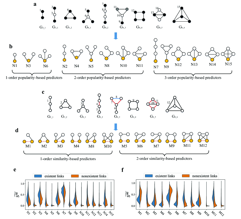
Figure 1: Graphlet orbits, orbit-degree-based link predictors, and orbit degree distribution. a Fifteen node orbits characterised by graphlets with 2–4 nodes. In each graphlet, nodes with different colours belong to different node orbits. b Fifteen popularity-based predictors, with the yellow node in each node orbit representing the endpoint of the target link for prediction. c Twelve edge orbits characterised by graphlets comprising 3–4 nodes. In each graphlet, edges with different colours belong to different edge orbits. d Twelve similarity-based predictors, with the dotted red line in each edge orbit representing the target link for prediction. e and f Distributions of normalized popularities $\widetilde{S^{Ni}_{xy}}=\frac{S^{Ni}_{\max}-S^{Ni}_{xy}}{S^{Ni}_{\max}-S^{Ni}_{\min}}$ and normalized similarities $\widetilde{S^{Mj}_{xy}}=\frac{S^{Mj}_{\max}-S^{Mj}_{xy}}{S^{Mj}_{\max}-S^{Mj}_{\min}}$ for existent and nonexistent links in a contact network of high school students, where $S^{Ni}_{\max}$ and $S^{Mj}_{\max}$ are maximum values over considered links for Eq. 7 and Eq. 8, respectively. For most orbit degrees, the distributions for existent and nonexistent links are visually distinct.

An isomorphism $f(\cdot)$ from graph $X$ to graph $Y$ is a bijection from the nodes of $X$ to the nodes of $Y$, such that if $(x,y)$ is an edge of $X$, then $(f(x),f(y))$ is an edge of $Y$. An automorphism $g(\cdot)$ is a special case of isomorphism in which a graph is mapped to itself. The set of all automorphisms of a graph $X$ forms the automorphism group of $X$, which is denoted by $Aut(X)$. For an arbitrary node $x$ in graph $X$, the automorphism orbit of $x$ in the automorphism group is expressed as follows:

$$Norb(x)=\{x^{\prime}\in V(X)|x^{\prime}=g(x)\},$$ (1)

where $V(X)$ is the set of nodes of graph $X$ and $g\in Aut(X)$. Similarly, the automorphism orbit of an edge $(x,y)$ in graph $X$ is expressed as follows:

$$Eorb((x,y))=\{(x^{\prime},y^{\prime})\in E(X)|x^{\prime}=g(x),y^{\prime}=g(y)\},$$ (2)

where $E(X)$ is the set of edges in graph $X$. In Fig. 1, the same gray level and colour are used to indicate nodes and edges in the same orbit. Graphlets comprising two to four nodes collectively encapsulate 15 distinctive node orbits (Fig. 1a) and 12 distinctive edge orbits (Fig. 1c). We only focused on graphlets comprising fewer than five nodes for two reasons. First, the calculation of orbit degrees associated with small graphlets has low computational complexity. Second, higher-order graphlets are typically composed of lower-order graphlets; the abundance of higher-order graphlets in a graph depends on the prevalence of the constitutive lower-order graphlets vazquez2004topological . A previous empirical study indicated that the structural configurations of graphlets with five or more nodes do not significantly influence the accuracy of link prediction chiang2011exploiting .

Studies employing subgraph models for link prediction have predominantly focused on motifs milo2002network ; zhang2013potential ; xia2019survey ; liu2019link ; liu2019link2 ; wang2020model ; li2021research ; xia2021chief ; backstrom2014romantic ; dong2017structural ; such studies have used the number of motifs that a targeted link participates in as a quantitative indicator for link prediction. However, motifs do not account for the varied roles of different edges within them, thereby ignoring edge orbits. Some studies milenkovic2008uncovering ; hulovatyy2014revealing ; feng2020link have utilised graphlets in link prediction; these studies have estimated the existing likelihood of target links by constructing a node or edge graphlet degree vector (GDV) on the basis of the number of graphlets that a node or an edge belongs to. However, nodes or edges belonging to the same graphlet but to different orbits have different structural roles. Therefore, in the present study, we focused on the frequency of each orbit and defined the node orbit degree and edge orbit degree. We then used the node orbit degree and edge orbit degree to quantify the multi-order popularity of a node and the multi-order similarity between two nodes, respectively.

The node orbit degree is defined as the number of graphlets containing a node that belongs to a specific node orbit prvzulj2007biological . For a specific graphlet $M$ in network $G$, we can assume that $n$ node sets $\{Norb_{1},Norb_{2},\cdots,Norb_{n}\}$ correspond to the $n$ different node orbits in $M$ and that $l$ instances of graphlet $M$ exist ($\{M^{1},M^{2},\cdots,M^{l}\}$). The node set corresponding to the $i$th node orbit in the $c$th instance can then be denoted as $Norb_{i}^{c}$. The node orbit degree of any node $x$ is expressed as follows:

$$NMD_{i}(x)=\sum\limits_{c=1}^{l}{N_{i}^{c}(x)},$$ (3)

where

$$N_{i}^{c}(x)=\begin{cases}1,&x\in Norb_{i}^{c}\\ 0,&otherwise\\ \end{cases}.$$ (4)

The edge orbit degree is defined as the number of graphlets containing an edge that belongs to a specific edge orbit solava2012graphlet . If $m$ edge sets correspond to $m$ different edge orbits in $M$, $Eorb_{j}^{c}$ represents the set of edges on the $j$th edge orbit in the $c$th instance, and the edge orbit degree of $e_{xy}$ is expressed as follows:

$$EMD_{j}(e_{xy})=\sum\limits_{c=1}^{l}{E_{j}^{c}(e_{xy})},$$ (5)

where

$$E_{j}^{c}(e_{xy})=\begin{cases}1,&e_{xy}\in Eorb_{j}^{c}\\ 0,&otherwise\\ \end{cases}.$$ (6)

This study derived a total of 15 multi-order popularity-based predictors relying on node orbit degrees, as displayed in Fig. 1b. In this figure, the yellow nodes represent the endpoints of the links to be predicted. The order of the aforementioned predictor is defined as the length of the longest path starting from the target node. For example, for N1$(\vbox{\hbox{\includegraphics[width=6.45831pt,height=12.05553pt]{./motif/N1.pdf}}})$, N3$(\vbox{\hbox{\includegraphics[width=12.05553pt,height=12.05553pt]{./motif/N3.pdf}}})$, and N6$(\vbox{\hbox{\includegraphics[width=12.05553pt,height=12.05553pt]{./motif/N6.pdf}}})$, the longest path length starting from the target node is 1; thus, these predictors are first-order popularity-based predictors. On the basis of this logic, N2$(\vbox{\hbox{\includegraphics[width=12.05553pt,height=12.05553pt]{./motif/N2.pdf}}})$ and N5$(\vbox{\hbox{\includegraphics[width=12.05553pt,height=12.05553pt]{./motif/N5.pdf}}})$ are second-order predictors, and N7$(\vbox{\hbox{\includegraphics[width=6.45831pt,height=12.05553pt]{./motif/N7.pdf}}})$ and N9$(\vbox{\hbox{\includegraphics[width=12.05553pt,height=12.05553pt]{./motif/N9.pdf}}})$ are third-order predictors. On the basis of the PA index, the product of the node orbit degrees of the two endpoints of a target link are used to estimate the likelihood of the target link’s existence; the relevant equation is as follows:

$$\begin{split}S^{Ni}_{xy}={N_{i}(x)}\cdot{N_{i}(y)},\end{split}$$ (7)

where $N_{i}(x)$ is the node orbit degree of node $x$ for $Ni$. The 15 predictors based on the node orbit degree are denoted as ${S^{N1},S^{N2},\cdots,S^{N15}}$.

This study also derived a total of 12 multi-order similarity-based predictors relying on edge orbit degrees, as illustrated in Fig. 1d. In this figure, the red dashed links represent target links (yellow node pairs) to be predicted. The order of the aforementioned predictor is defined as the length of the longest path that starts from any one endpoint but does not reach the other endpoint. For example, the predictors M1$(\vbox{\hbox{\includegraphics[width=12.05553pt,height=12.05553pt]{./motif/M1.pdf}}})$ and M2$(\vbox{\hbox{\includegraphics[width=12.05553pt,height=12.05553pt]{./motif/M2.pdf}}})$ are first-order similarity-based predictors because the longest path starting from one of their endpoints but not reaching the other endpoint is 1. On the basis of this logic, M5$(\vbox{\hbox{\includegraphics[width=12.05553pt,height=12.05553pt]{./motif/M5.pdf}}})$ and M9$(\vbox{\hbox{\includegraphics[width=12.05553pt,height=12.05553pt]{./motif/M9.pdf}}})$ are second-order predictors. On the basis of the CN index, edge orbit degrees are treated as similarity-based scores for the target node pair and expressed as follows:

$$\begin{split}S^{Mj}_{xy}=M_{j}(x,y),\end{split}$$ (8)

where $M_{j}(x,y)$ is the edge orbit degree of edge $(x,y)$ for $Mj$. The 12 predictors base on the edge orbit degree are denoted as $S^{M1},S^{M2},\cdots,S^{M12}$. The algorithmic calculation and computational complexity for the node and edge orbit degrees are detailed in Supplementary Note 1.

In traditional link prediction approaches, a higher link score always indicates a higher likelihood of link existence; however, in the proposed approach, a higher score might imply a lower likelihood of link existence for certain orbit degrees. In our approach, each orbit degree is treated as a one-dimensional feature, and link prediction is conducted using a supervised binary classification model. Therefore, whether a feature contributes positively or negatively to the existence likelihood is secondary to its effectiveness in distinguishing between an existing link and a nonexistent one. Accordingly, a feature that aids in this differentiation facilitates link prediction even if a larger value of the feature corresponds to a lower likelihood of link existence.

To provide a clear understanding of the functions of orbit degrees in link prediction, the distributions of orbit-degree-based scores of node pairs were compared for existing and nonexistent links in a contact network of high school students fournet2014contact (Fig. 1e). Scores based on the node and edge orbit degrees were calculated using Eqs. 7 and 8, respectively. These distributions were visualised using violin plots, which indicated that the distributions of orbit-degree-based scores for existing and nonexistent links are remarkably different.

Orbit-degree representations of existing multi-order popularity- and similarity-based methods. The proposed orbit-degree-based approach provides a systematic framework for using popularity- and similarity-based indices in link prediction. Many well-known popularity- and similarity-based methods can be regarded as orbit degree methods. The following text details how certain popular indices can be expressed in orbit degrees.

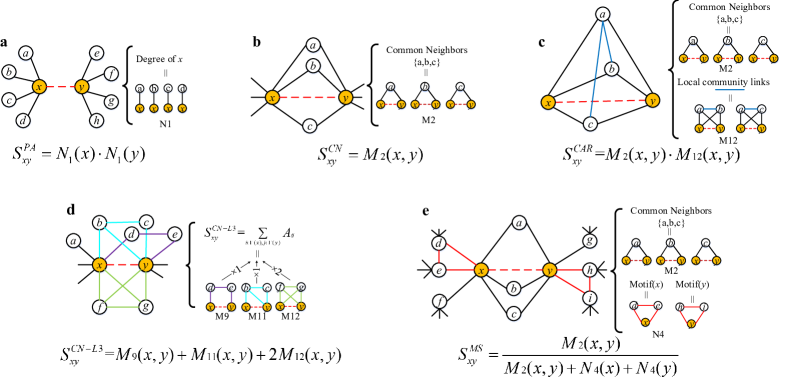
Figure 2: Decomposing popularity- and similarity-based indices by orbit degrees. a The degrees of nodes $x$ and $y$ are captured by orbit N1. Thus, the PA index of these nodes is simply the product of their numbers of N1 orbits. b The CN index indicates the number of CN for nodes $x$ and $y$, which is reflected by M2. c The CAR index depends on M2, which reflects the CN, and M12, which represents the local community links. d The CN-L3 score indicates the combined effects of edge orbits M9, M11, and M12 around nodes $x$ and $y$, with each M9 or M11 orbit contributing 1 to this score and each M12 orbit contributing 2 to the score. e The motif-based similarity index indicates the similarity between nodes $x$ and $y$; this similarity is determined on the basis of the CN of and triangles formed by these nodes, which can be fully represented by M2 and N4, respectively.

The PA index is a first-order popularity metric barabasi1999emergence that is expressed as follows:

$$S_{xy}^{PA}={k_{x}}\cdot{k_{y}},$$ (9)

where $k_{x}$ and $k_{y}$ are the degrees of nodes $x$ and $y$, respectively. The degree of node $x$ is equivalent to the degree of node orbit $N_{1}(x)$ because N1$(\vbox{\hbox{\includegraphics[width=6.45831pt,height=12.05553pt]{./motif/N1.pdf}}})$ represents the number of first-order neighbors of this node (Fig. 2a). Therefore, the PA index can be rewritten as follows:

$$S_{xy}^{PA}={N_{1}(x)}\cdot{N_{1}(y)}.$$ (10)

The CN index is the most commonly used local similarity index in link prediction liben2007link . This index measures the number of CN of a pair of nodes. If $\Gamma(x)$ denotes the neighbor set of any node $x$, then the CN index can be expressed as follows:

$$\begin{split}S_{xy}^{CN}=\left|{\Gamma(x)\cap\Gamma(y)}\right|.\end{split}$$ (11)

Determining the edge orbit degree M2$(\vbox{\hbox{\includegraphics[width=12.05553pt,height=12.05553pt]{./motif/M2.pdf}}})$ of two target edges $x$ and $y$ is equivalent to determining the number of CN for them (Fig. 2b). Therefore, the CN index can be reformulated as follows:

$$S_{xy}^{CN}=M_{2}(x,y).$$ (12)

On the basis of the preceding equation, the Adamic–Adar (AA) index adamic2003friends and resource allocation (RA) index zhou2009predicting , which are popular variants of the CN index, can be formulated in terms of orbit degrees as follows:

$$S_{xy}^{AA}=\sum_{z\in\Gamma(x)\cap\Gamma(y)}\frac{1}{\log N_{1}(z)},$$ (13)

and

$$S_{xy}^{RA}=\sum_{z\in\Gamma(x)\cap\Gamma(y)}\frac{1}{N_{1}(z)}.$$ (14)

The CN, AA, and RA indices are first-order similarity indices. Another variant of the CN index is the CAR index cannistraci2013link , which accounts for the role of the local community of CN (i.e., second-order similarity). The CAR index is expressed as follows:

$$S_{xy}^{CAR}=S_{xy}^{CN}\cdot\sum_{z\in\Gamma(x)\cap\Gamma(y)}\frac{|\gamma(z)|}{2},$$ (15)

where $\gamma(z)$ denotes the neighbors of $z$ that are also neighbors to $x$ and $y$. The term $S_{xy}^{CN}$ is equivalent to $M_{2}(x,y)$, and $\sum_{z\in\Gamma(x)\cap\Gamma(y)}\frac{|\gamma(z)|}{2}$ is the number of links connecting the CN of $x$ and $y$; the term $\sum_{z\in\Gamma(x)\cap\Gamma(y)}\frac{|\gamma(z)|}{2}$ is equivalent to the number of M12$(\vbox{\hbox{\includegraphics[width=12.05553pt,height=12.05553pt]{./motif/M12.pdf}}})$ orbits when $(x,y)$ is the target link (see Fig. 2c). Therefore, the CAR can be rewritten as follows:

$$S_{xy}^{CAR}=M_{2}(x,y)\cdot M_{12}(x,y).$$ (16)

In addition to first-order similarity indices, which incorporate information from two-hop paths, second-order similarity indices are used in the proposed method. Second-order similarity indices incorporate information from three-hop paths zhou2009predicting ; lu2009similarity ; kovacs2019network ; zhou2021experimental and can be expressed using second-order edge orbit degrees. The second-order similarity index used in the proposed method is the CN-L3 index kovacs2019network ; zhou2021experimental . This index indicates the number of three-hop paths between the target node pair and is expressed as follows:

$$\begin{split}S_{xy}^{CN-L{\rm{3}}}{\rm{=}}\sum\limits_{i\in\Gamma(x),j\in\Gamma(y)}{{A_{ij}}},\end{split}$$ (17)

where $A$ is the adjacency matrix. If $i$ and $j$ are directly connected, $A_{ij}=1$; otherwise, $A_{ij}=0$. As illustrated in Fig. 2d, the CN-L3 index can be interpreted as a linear combination of the edge orbit degrees M9$(\vbox{\hbox{\includegraphics[width=12.05553pt,height=12.05553pt]{./motif/M9.pdf}}})$, M11$(\vbox{\hbox{\includegraphics[width=12.05553pt,height=12.05553pt]{./motif/M11.pdf}}})$, and M12$(\vbox{\hbox{\includegraphics[width=12.05553pt,height=12.05553pt]{./motif/M12.pdf}}})$. In M9$(\vbox{\hbox{\includegraphics[width=12.05553pt,height=12.05553pt]{./motif/M9.pdf}}})$ or M11$(\vbox{\hbox{\includegraphics[width=12.05553pt,height=12.05553pt]{./motif/M11.pdf}}})$, one 3-hop path connects nodes $x$ and $y$, whereas in M12$(\vbox{\hbox{\includegraphics[width=12.05553pt,height=12.05553pt]{./motif/M12.pdf}}})$, two such paths exist; thus, the CN-L3 index can be rewritten in terms of second-order edge orbit degrees as follows:

$$S_{xy}^{CN-L{\rm{3}}}=M_{9}(x,y)+M_{11}(x,y)+2M_{12}(x,y).$$ (18)

Indices based on PA and CN account for only popularity and similarity, respectively. By contrast, the motif-based similarity (MS) index li2021research accounts for both popularity and similarity. In this index, the triangular motifs associated with the target node pair is considered as follows:

$$S_{xy}^{MS}=\frac{{\left|{\Gamma(x)\cap\Gamma(y)}\right|}}{{\left|{\Gamma(x)\cap\Gamma(y)}\right|+motif(x)+motif(y)}},$$ (19)

where $motif(x)$ represents the number of triangular motifs that include node $x$ (i.e., the popularity of node $x$). This number is equal to the node orbit degree N4$(\vbox{\hbox{\includegraphics[width=14.2083pt,height=14.2083pt]{./motif/N4.pdf}}})$ of $x$ (Fig. 2e). Therefore, the MS index can be expressed in terms of orbit degrees as follows:

$$S_{xy}^{MS}=\frac{M_{2}(x,y)}{{M_{2}(x,y)+N_{4}(x)+N_{4}(y)}}.$$ (20)

In summary, popular multi-order popularity- and similarity-based indices can be represented in terms of orbit degrees; however, some structural characteristics that can be captured by orbit degrees have not been incorporated into any popularity- or similarity-based indices in the literature. Therefore, using orbit degrees as features in suitable machine learning methods can improve the accuracy of link prediction. Moreover, orbit degrees can indicate the roles of multi-order popularity and similarity mechanisms in link prediction for networks.

Performance Evaluation. We used the proposed method on 550 undirected and unweighted real-world networks from various domains (see Materials and Methods). Herein, a network is denoted by $G(V,E)$, where $V$ and $E$ represent the sets of nodes and links, respectively. In each implementation of a network ($G$), its link set $E$ was randomly divided into three parts ($E=E^{Tr}\cup E^{Va}\cup E^{Te}$) at a ratio of 8:1:1 for training, validation, and testing, respectively. The training set $E^{Tr}$ and validation set $E^{Va}$ contained known information, whereas the test set $E^{Te}$ contained unknown data. Parametric models were trained on $E^{Tr}$, and the model parameters were determined through link prediction for $E^{Va}$. Subsequently, we combined the training and validation sets (i.e., $E^{Tr}\cup E^{Va}$) and used the parametric models with estimated parameters to predict links for $E^{Te}$. For parameter-free models (such as the CN and RA models), we directly used different similarity indices by using data from $E^{Tr}\cup E^{Va}$ and then predicted links for $E^{Te}$. The aforementioned procedure is a standard process in machine learning and provides more reliable results than do traditional methods (see, for example, the procedure described in lu2011link ) in which $E^{Te}$ is used to determine parameters, which results in the information in $E^{Te}$ no longer being unknown for the algorithm. To mitigate the errors introduced by the highly imbalanced ratio between positive and negative samples in the training set, we employed a negative sampling technique goldberg2014word2vec ; yang2020understanding . Specifically, we regarded the sets $E^{Va}$ and $E^{Te}$ as containing positive samples (missing links) and randomly selected two subsets from the set $U-E$ ($U$ denotes the universal set containing all $|V||V-1|/2$ potential links) to serve as negative samples in each run; these subsets had sizes equal to those of $E^{Va}$ and $E^{Te}$. Consequently, in calibrating model parameters and assessing algorithm performance, the present link prediction task was transformed into a binary classification problem with an equal number of positive and negative samples.

We developed an orbit-degree-based model by using XGBoost, which is a commonly used supervised learning model for binary classification chen2016xgboost ; lei2022forecasting , to fuse all node and edge orbit degrees; each orbit degree was considered a one-dimensional input feature. The results obtained using only node orbit degrees and only edge orbit degrees in XGBoost are presented in Supplementary Note 2; these results were poor. The performance of the proposed model was compared with that of nine structure-based models and three embedding-based ones. The nine adopted structure-based models comprised models applying the PA index barabasi1999emergence , CN index liben2007link , RA index zhou2009predicting , CN-L3 index zhou2021experimental , RA-L3 index zhou2021experimental , CAR index cannistraci2013link , Katz index (a global similarity index; katz1953new ), MS index li2021research , and node–GDV index milenkovic2008uncovering . To conduct a fair comparison, the similarity index was treated as an input feature for XGBoost in each structure-based model. The three adopted embedding-based models were DeepWalk perozzi2014deepwalk , node2vec grover2016node2vec , and GraphWave donnat2018learning .

Table 1 presents the results obtained with the compared models for 550 real-world networks; the top-performing model is presented in bold. The performance of these models was evaluated using four classification metrics, namely area under the receiver operating characteristic curve (AUC), precision, recall, and F1-score (see Materials and Methods). Overall, the proposed model outperformed the other models in terms of all evaluation metrics. All structure-based models, except for that using the Katz index, consider only a subset of the features considered in the proposed model; thus, their performance was inferior to that of the proposed model. The model using the Katz index accounts for all paths, and it outperformed all models except for the proposed model in terms of AUC, recall, and F1-score. Compared with the model using the Katz index, the proposed model had an 11.4% higher AUC, a 4.9% higher recall, and an 8.7% higher F1-score. This result indicates that laboriously mining global information is unnecessary in link prediction; instead, local information can be leveraged by appropriately fusing node and edge orbit degrees. The RA-L3 model exhibited the highest precision among all benchmark models; however, the proposed model had a 4.8% higher precision than did this model. The proposed model substantially outperformed the three embedding-based models. Among the three embedding-based models, node2vec exhibited the best performance. Compared with node2vec, DeepWalk exhibited lower classification performance, possibly because of its flexible neighborhood sampling strategy. Finally, GraphWave exhibited the lowest performance among the embedding-based models, potentially because of its incompatibility with the link prediction task cao2019network .

Table 1: Performance (mean $\pm$ standard deviation) of the proposed model and some selected benchmark models in terms of AUC, precision, recall, and F1-score. The presented results are average values obtained for 550 real-world networks, with 10 independent runs implemented for each network.

Methods		AUC	Precision	Recall	F1-score
Structure-based	PA barabasi1999emergence	0.696 $\pm$ 0.106	0.649 $\pm$ 0.119	0.668 $\pm$ 0.171	0.650 $\pm$ 0.125
	CN liben2007link	0.675 $\pm$ 0.194	0.622 $\pm$ 0.358	0.603 $\pm$ 0.412	0.554 $\pm$ 0.346
	RA zhou2009predicting	0.672 $\pm$ 0.193	0.630 $\pm$ 0.363	0.595 $\pm$ 0.412	0.550 $\pm$ 0.346
	CN-L3 zhou2021experimental	0.707 $\pm$ 0.182	0.749 $\pm$ 0.290	0.561 $\pm$ 0.369	0.566 $\pm$ 0.320
	RA-L3 zhou2021experimental	0.711 $\pm$ 0.183	0.762 $\pm$ 0.288	0.561 $\pm$ 0.367	0.570 $\pm$ 0.322
	CAR cannistraci2013link	0.667 $\pm$ 0.190	0.618 $\pm$ 0.360	0.593 $\pm$ 0.412	0.545 $\pm$ 0.345
	Katz katz1953new	0.766 $\pm$ 0.148	0.713 $\pm$ 0.166	0.767 $\pm$ 0.167	0.734 $\pm$ 0.155
	MS li2021research	0.669 $\pm$ 0.191	0.625 $\pm$ 0.362	0.592 $\pm$ 0.413	0.546 $\pm$ 0.345
	Node-GDV milenkovic2008uncovering	0.706 $\pm$ 0.101	0.657 $\pm$ 0.104	0.658 $\pm$ 0.129	0.652 $\pm$ 0.099
Embedding-based	DeepWalk perozzi2014deepwalk	0.707 $\pm$ 0.108	0.648 $\pm$ 0.136	0.624 $\pm$ 0.135	0.610 $\pm$ 0.132
	Node2vec grover2016node2vec	0.727 $\pm$ 0.172	0.683 $\pm$ 0.182	0.693 $\pm$ 0.193	0.683 $\pm$ 0.182
	GraphWave donnat2018learning	0.536 $\pm$ 0.078	0.515 $\pm$ 0.096	0.528 $\pm$ 0.143	0.515 $\pm$ 0.102
Proposed	OD	0.854 $\pm$ 0.130	0.799 $\pm$ 0.150	0.805 $\pm$ 0.152	0.798 $\pm$ 0.143

Feature analyses. To thoroughly analyse the roles of popularity and similarity mechanisms in networks, we used the XGBoost model to integrate all node and edge orbit degree features and employed Shapley additive explanations (SHAP) values (see Materials and Methods) to quantify the importance of each feature. A higher mean absolute SHAP value indicates higher feature importance, and an increase in the positive or negative mean SHAP value of a feature indicates that as the value of this feature increases, the likelihood of the model generating a positive- or negative-class prediction increases, respectively. Fig. 3a displays the top 10 features based on mean absolute SHAP values for the board membership network of Norwegian public limited companies. In this network, two directors were linked if they shared membership in at least one board of directors. The two highest-ranked features, namely M2$(\vbox{\hbox{\includegraphics[width=12.05553pt,height=12.05553pt]{./motif/M2.pdf}}})$ and M4$(\vbox{\hbox{\includegraphics[width=12.05553pt,height=12.05553pt]{./motif/M4.pdf}}})$, were determined to be similarity-based features, and their mean absolute SHAP values were considerably larger than that of the third ranked feature. Thus, the similarity mechanism played a predominant role in the formation of the aforementioned network. Fig. 3b depicts the SHAP values of the top 10 features for all positive and negative samples. In this figure, the colour of a data point indicates the magnitude of the feature value of the sample. If the SHAP value tended to be positive for a higher feature value (indicated by red in Fig. 3b), then the corresponding orbit degree played a positive role in the existence of a missing link; however, if the SHAP value tends to be negative for higher feature values, the corresponding orbit degree can be considered to play a negative role in the existence of a missing link. For the social network analysed in this subsection, an increase in the value of $M_{2}(x,y)$ increased the probability that $(x,y)$ was a missing link; by contrast, an increase in the value of $M_{4}(x,y)$ decreased the probability that $(x,y)$ was a missing link. The detailed quantitative analysis for the aforementioned network is provided in Supplementary Note 3. In summary, the key orbit degree features in any network can be identified by evaluating the absolute SHAP values of all features. The absolute SHAP value of each feature represents the feature importance, and the sign of this value indicates the direction of the effect of the feature on the predicted outcome.

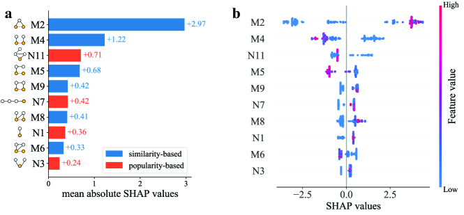
Figure 3: Results of feature analyses for the board membership network of Norwegian public limited companies. a Top 10 features for the XGBoost model (determined on the basis of mean absolute SHAP values). The blue and orange colours denote similarity- and popularity-based features, respectively. The two highest-ranked features, namely M2 and M4, are similarity-based features, which indicates the dominant role of similarity mechanisms in link formation in the examined network. b SHAP values of the top 10 features for all positive and negative samples, with the colours of data points reflecting the feature values of corresponding samples.

Domain analyses. The results obtained for the board membership network of Norwegian public limited companies indicate that M2$(\vbox{\hbox{\includegraphics[width=12.05553pt,height=12.05553pt]{./motif/M2.pdf}}})$ was the most important feature in this network. Moreover, similarity-based mechanisms were more crucial for link predictions in the aforementioned network than were popularity-based mechanism. For the board membership network of Norwegian public limited companies, M2$(\vbox{\hbox{\includegraphics[width=12.05553pt,height=12.05553pt]{./motif/M2.pdf}}})$ had the highest mean absolute SHAP value and positive mean SHAP value. Thus, the homophily mechanism mcpherson2001birds plays a critical role in the formation of this network. In summary, the dominant features of a given network can be analysed to gain valuable insights into how the network is structured. Network topological characteristics vary considerably across different domains newman2003social ; estrada2007topological , and large-scale empirical studies have indicated that link prediction algorithms exhibit significant performance disparities when they are applied to networks from different domains ghasemian2020stacking ; zhou2021experimental ; muscoloni2023stealing . Therefore, we investigated whether similarity and popularity mechanisms (represented by orbit degrees) play different roles in link prediction for networks in different domains. First, we represented each real network by a 27-dimensional vector in which each element represented the SHAP value of the corresponding orbit degree (27 elements, namely N1–N15 and M1–M12). Subsequently, we conducted principal component analysis (PCA) hotelling1933analysis to reduce the 550 twenty-seven-dimensional vectors into two-dimensional vectors. As displayed in the PCA scatter plot (Fig. 4a), social and economic networks were closely clustered, biological and information networks were dispersed, and transportation and technological networks were moderately clustered. We used the average distance between pairwise networks in the PCA scatter plot to quantify the degree of clustering of networks in a domain; moreover, we compared real data and the null model when domain labels were completely randomly shuffled (see Materials and Methods). As presented in Table 2, networks in all domains except for the biological and information ones had higher degrees of clustering than did networks in the null model. A comparison of $\overline{D}$ for different domains indicated that social and economic networks had the highest degree of clustering, which is consistent with Fig. 4a.

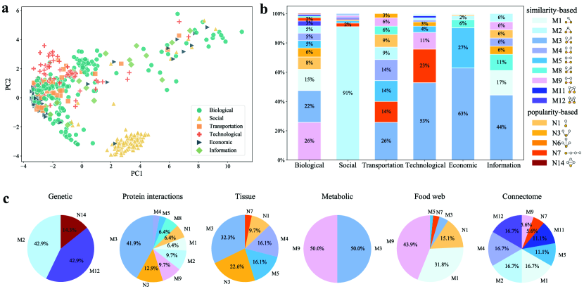
Figure 4: Different feature roles in networks from different domains. a PCA scatter plot of networks. In this scatter plot, each network is represented by a 27-dimensional vector composed of 27 SHAP values corresponding to the 27 orbit degrees. After these vectors are reduced to two-dimensional ones, data points (corresponding to networks) are visualised with different colours representing different domains. b Variations in the win rate with mean absolute SHAP values for all features in six examined domains. Features based on similarity mechanisms are depicted in shades of blue, whereas those based on popularity mechanisms are shown in shades of orange. c Win rates across all features in biological networks with different subdomains.

Table 2: Degree of clustering of networks from various domains. $\overline{D}$ represents the clustering degree of real networks within each domain, while $\langle\tilde{D}\rangle$ denotes the average degree of clustering for the null model over 100 independent runs.

Domain	$\overline{D}$	$\langle\tilde{D}\rangle$	$p$-value
Biological	4.215	4.537	0.03
Social	1.961	4.513	$<$0.01
Transportation	2.568	4.461	$<$0.01
Technological	2.386	4.579	$<$0.01
Economic	1.882	4.497	$<$0.01
information	4.371	4.596	0.39

We also examined the first ranking feature for each network (determined on the basis of the mean absolute SHAP value). Fig. 4b displays the win rates for all features in the six examined domains. In 113 of the 124 analysed social networks, M2$\left(\vbox{\hbox{\includegraphics[width=12.05553pt,height=12.05553pt]{./motif/M2.pdf}}}\right)$ had the highest mean absolute SHAP value among all 27 features; thus, the win rate of M2$\left(\vbox{\hbox{\includegraphics[width=12.05553pt,height=12.05553pt]{./motif/M2.pdf}}}\right)$ in social networks was $113/124\approx 0.91$. This result indicates that the homophily mechanism plays a critical role in the formation of social networks. For the technological, economic, and information networks, M3$\left(\vbox{\hbox{\includegraphics[width=12.05553pt,height=12.05553pt]{./motif/M3.pdf}}}\right)$ was the top ranking feature, with its win rates being 53%, 63%, and 44%, respectively. By contrast, no top ranking feature was identified for the biological and transportation networks. As displayed in Fig. 4c, biological networks from different subdomains had different top ranking features, resulting in a broad distribution of important features for the biological domain. A similar scenario was observed for the transportation networks. Details regarding the subdomain analysis are provided in Supplementary Note 4.

Discussion

The proposed orbit-degree-based model quantifies multi-order popularity and multi-order similarity by using node orbit degrees and edge orbit degrees, respectively. Thus, the proposed model can use both low- and high-order features for link prediction. Specifically, some low-order features (e.g., the PA index and CN index) directly correspond to individual orbit degree features, whereas high-order features (e.g., the CN-L3 and CAR indices) can be represented by combining a few orbit degree features (see Fig. 2). We achieve accurate link prediction performance by using orbit degrees as features in the XGBoost model (see Table 1). Our results reveal that adding popularity features (node orbit degree) to similarity features (edge orbit degree) can only marginally improve model performance (see Table 1 and Supplementary Table S2). This finding suggests that similarity features play a more crucial role in link prediction than do popularity features, partially because similarity features contain some popularity information.

We identified the roles of individual features in link prediction across various domains by calculating the features’ mean absolute SHAP values in the XGBoost model. Among the 124 examined social networks, M2$(\vbox{\hbox{\includegraphics[width=12.05553pt,height=12.05553pt]{./motif/M2.pdf}}})$, which represents the homophily mechanism, was the most important mechanism in 113 networks, with its win rate being 91%. This result indicates that the homophily mechanism plays a dominant role in the formation of social networks. In the analysed economic, technological, and information networks, M3$(\vbox{\hbox{\includegraphics[width=12.05553pt,height=12.05553pt]{./motif/M3.pdf}}})$ had the highest win rate. This feature is a similarity feature but contains some popularity information. As mentioned in Supplementary Note 5, M3 is closely related to but different from the PA index, and it exhibits high win rates for networks with abundant star-like structures. In contrast to the aforementioned networks, no single top ranking feature was identified for the examined biological and transportation networks (see Fig. 4b). An analysis of the subdomains of these networks revealed considerable variations in the top ranking features of networks from different sudomains (see Fig. 4c and Supplementary Note 4). This finding highlights the complexity of network formation mechanisms in these biological and transportation domains.

Our study has two limitations. First, we assessed the roles of multi-order popularity and similarity features by simply comparing mean absolute SHAP values rather than conducting an in-depth domain-specific analysis. The roles of some important features, such as M2$(\vbox{\hbox{\includegraphics[width=12.05553pt,height=12.05553pt]{./motif/M2.pdf}}})$ and M3$(\vbox{\hbox{\includegraphics[width=12.05553pt,height=12.05553pt]{./motif/M3.pdf}}})$, are relatively easily to understand; however, the roles of other important features are not fully clear. Therefore, future studies should use domain-specific knowledge to conduct in-depth analyses of the roles played by features with high SHAP values in the formation of networks in different domains. Second, our study focused on simple networks; however, real systems might be more effectively described by weighted networks barrat2004architecture , directed networks garlaschelli2004patterns , temporal networks holme2012temporal , spatial networksbarthelemy2011spatial , and higher-order networksbick2023higher . Therefore, in the future, we intend to extend the proposed orbit-degree-based framework to the aforementioned complex networks.

In summary, the proposed model considers the structural heterogeneity of nodes and edges within graphlets to achieve high prediction and interpretation performance in link prediction. The applications of graphlets are not limited to link prediction tasks. For example, the spreading capabilities of different nodes can be identified on the basis of the heterogeneity of subgraphs to construct more precise spreading models benson2018simplicial ; iacopini2019simplicial . Therefore, the proposed model can have broad applications in network science.

Materials and Methods

Data description. We conducted extensive experiments on a vast and structurally diverse corpus of 550 real-world networks ghasemian2020stacking , which represents a slightly expanded version of the CommunityFitNet corpus ghasemian2019evaluating . The network data for this study were obtained from the Index of Complex Networks. Among the 550 considered networks, 124 (23%) were social networks, 179 (32%) were biological networks, 124 (23%) were economic networks, 67 (12%) were technological networks, 18 (3%) were information networks, and 38 (7%) were transportation networks. These networks have considerably different sizes, with the difference being up to three orders of magnitude. The diversity in the domains and sizes of the networks considered in the present study makes the data set of this study one of the most comprehensive and varied benchmark data sets for link prediction. This data set enabled us to conduct thorough comparisons of link prediction methods across various domains, which provided valuable insights into the domain-specific performance of different methods and features.

Evaluation metrics. We adopted four standard binary classification metrics to evaluate the link prediction performance of different models: AUC, precision, recall, and F1-score. AUC hanley1982meaning ; bradley1997use indicates the ability of a model to discriminate between positive and negative classes across all possible classification thresholds. This metric is the most frequently used performance measures in link prediction (see Table 1 in the study of zhou2023discriminating ), probably because it has high interpretability, can be easily visualised, and exhibits high discrimination ability bradley1997use ; zhou2023discriminating ; jiao2024comparing . However, some researchers have argued that AUC is unsuitable for evaluating imbalanced classification problems yang2015evaluating ; saito2015precision . In this study, we adopted a negative sampling technique to generate balanced positive and negative classes so that AUC could be used to evaluate model performance. In this study, AUC could be interpreted as representing the probability that randomly selected positive samples (missing links) had higher probabilities of being predicted as positive samples by a feature-trained XGBoost model when compared with randomly selected negative samples (nonexistent links). The AUC value should be 0.5 if all scores of predicted links are randomly generated from an independent and identical distribution; thus, AUC values above 0.5 indicate that the model predictions are more accurate than random predictions.

Model predictions can be classified into four categories: (1) true positives (TP), which refer to correctly predicted positive samples (missing links in this study); (2) false positives (FP), which refer to incorrectly predicted positive samples (nonexistent links predicted to be missing); (3) true negatives (TN), which refer to correctly predicted negative samples (nonexistent links predicted to be nonexistent); and (4) false negatives (FN), which refer to incorrectly predicted negative samples (missing links predicted to be nonexistent). Precision buckland1994relationship indicates the accuracy of the positive predictions of a model and can be calculated as follows:

$$\text{Precision}=\frac{TP}{TP+FP}.$$ (21)

Recall buckland1994relationship indicates a model’s ability to identify all positive samples and is expressed as follows:

$$\text{Recall}=\frac{TP}{TP+FN}.$$ (22)

F1-score sasaki2007truth is defined as the harmonic mean of precision and recall and is expressed as follows:

$$F1\text{-}score=2\times\frac{\text{Precision}\times\text{Recall}}{\text{Precision}+\text{Recall}}.$$ (23)

Notice that it is strictly proved that if Precision, Recall, and F1-score adopt the same threshold to predict missing links (i.e., they all treat top-$L$ link with highest scores as missing links), they will give exactly the same ranking of evaluated algorithms bi2024inconsistency . However, this work employs a supervised learning framework where each algorithm is tasked with categorizing each sample in the test set as either a positive or negative instance, rather than ranking them based on the probability of being a positive sample. Consequently, different algorithms may not have consistent threshold values for their output results, implying that Precision, Recall, and F1-score could potentially yield differing rankings for these algorithms. In addition, the ranking of algorithms according to AUC is not strongly consistent with the ranking produced by representative threshold-dependent metrics like Precision and Recall (the correlation between AUC and a representative threshold-dependent metric typically ranges from 0.3 to 0.6, measured by the Spearman rank correlation coefficient bi2024inconsistency ). Therefore, if an algorithm is deemed the best performer across all these metrics, the conclusion about its superiority becomes more robust compared to evaluations based on a single metric alone.

SHAP values. SHAP values originate from the field of cooperative game theory, which was introduced by the economist Lloyd Shapley in 1953 shapley1953value . In the context of machine learning, SHAP values can explain the contribution of each feature to model predictions lundberg2017unified ; meng2021makes . Thus, SHAP values indicate feature importance. Specifically, for a given sample $x$, the SHAP value $\phi_{i}(x)$ of feature $i$ is calculated as the weighted average of the contributions of feature $i$ to model predictions across all possible feature combinations. The condition $\phi_{i}(x)>0$ implies that feature $i$ has a positive contribution to the model prediction for sample $x$, whereas $\phi_{i}(x)<0$ suggests that feature $i$ has a negative effect on the model’s output. The SHAP value is expressed as follows:

$$\phi_{i}(x)=\sum_{S\subseteq F\setminus\{i\}}\frac{|S|!(|F|-|S|-1)!}{|F|!}\left[f_{S\cup\{i\}}(x_{S\cup\{i\}})-f_{S}(x_{S})\right],$$ (24)

where $F$ denotes the set of all features and $S$ is a subset of $F$ that does not include feature $i$. The function $f$ represents the prediction model, and $x_{S}$ is the value of sample $x$ when the features in set $S$ are considered. The term $f_{S\cup\{i\}}(x_{S\cup\{i\}})$ represents the model prediction when the features in $S$ and feature $i$ are present in the model, whereas $f_{S}(x_{S})$ represents the model prediction when only the features in $S$ are present in the model. The SHAP value of feature $i$ is the sum of the SHAP values $\phi_{i}(x)$ for all samples $x$.

In our experiments, the SHAP value indicated the contribution of each feature to the probability of the model predicting a positive sample (missing link). We used the positive and negative samples from the test set to compute the SHAP value of each feature.

Clustering in the PCA scatter plot. If $d_{ij}$ denotes the Euclidean distance between data points $i$ and $j$ in the two-dimensional PCA scatter plot illustrated in Fig. 4a, the degree of clustering of a set of networks $Q$ can be quantified in terms of the average distance between these networks as follows:

$$\overline{D}_{Q}=\frac{1}{n(n-1)}\sum_{i,j\in Q,i\neq j}d_{ij}.$$ (25)

To investigate the degree of clustering of a given domain of networks $Q$, the corresponding $\overline{D}_{Q}$ value can be compared with those of other domains and that of a null model. The null model can be obtained by randomly shuffling domain labels. For domain $Q$, the degree of clustering of the null model, which is denoted by $\tilde{D}_{Q}$, can be obtained by randomly selecting $|Q|$ data points in the PCA plane and then calculating the average distance between these points. If $\tilde{D}_{Q}$ is significantly larger than $\overline{D}_{Q}$, the networks in domain $Q$ can be clustered. We performed $S$ independent runs to generate the null model and compared $\overline{D}$ and $\tilde{D}$ for each domain. For any domain $Q$, if the condition $\overline{D}_{Q}\leq\tilde{D}_{Q}$ occurs $s$ times, the corresponding $p$ value can be determined to be $s/S$; if this condition never occurs, then $p<1/S$.

Data availability

The relevant data sets were collected from public sources and will be publicly available at GitHub upon publication.

Author contributions

T.Z. and X.-K.X. conceptualised the research. Y.H. and Y.R. performed the research. Y.H., Y.R., Z.D., T.Z., and X.-K.X. analysed the collected data. Y.H., T.Z., and X.-K.X. wrote the manuscript. Y.R. and Z.D. edited the manuscript.

Competing financial interests

The authors declare no competing financial interests.

Supplementary Information:
Uncovering multi-order Popularity and Similarity Mechanisms in Link Prediction by graphlet predictors

Yong-Jian He, Yijun Ran, Zengru Di, Tao Zhou^∗, and Xiao-Ke Xu^∗

^∗To whom correspondence should be addressed: zhutou@ustc.edu,xuxiaoke@foxmail.com

Supplementary Note 1:   Algorithm implementation and complexity analysis

Here, we provide a specific implementation of the algorithms to obtain node and edge orbit degrees, along with an analysis of corresponding time complexity.

Node orbit degrees. The calculation of node orbit degrees can be implemented by algorithm ‣ Supplementary Note 1:. Assuming that there are $n$ nodes in the network $G$ and the maximum degree of the nodes is $d_{max}$ ($d_{max}\ll n$). First, we need to enumerate all nodes, and then for the $k$-node graphlets, we need to enumerate the neighbors of nodes with $k-1$ times. Therefore, the time complexities of link prediction based on node orbit degrees of 2-node, 3-node, and 4-node graphlets are $O(nd_{max})$, $O(nd_{max}^{2})$ and $O(nd_{max}^{3})$, respectively.

  Algorithm 1 Single node orbit degree

 

0:  $G(V,E)$ : the undirected network       $x$ : the endpoint of predicted edge.       $Ni$ : the node orbit degree feature

0:  $r_{a}^{{}^{\prime}}$ : the node orbit degree of node $x$ for $Ni$ $Nei(a)$ $\leftarrow$ the set of neighbors of any node $a$ in $G$ Initialize $N1_{num}$ = $N2_{num}$ = $\cdots$ = $N15_{num}$ = 0 For each node $b$ in $Nei(x)$ If node $b$ is connected to node $x$ do     $N1_{num}$ += 1 For each node $c$ in $Nei(b)$   If there are links between nodes $b$ and $x$, $c$ and $b$, and no link between $c$ and $x$ do     $N2_{num}$ += 1     ⋮  Else If there are links between nodes $b$ and $x$, $c$ and $x$, $b$ and $c$ do     $N4_{num}$ += 1   For each node $d$ in $Nei(c)$     If there are links between nodes $b$ and $x$, $c$ and $b$, $d$ and $b$, and no links between $c$ and $x$, $d$ and $x$, $c$ and $d$ do       $N5_{num}$ += 1       ⋮    Else If there are links between nodes $b$ and $x$, $c$ and $x$, $d$ and $x$, $b$ and $c$, $b$ and $d$, $c$ and $d$ do       $N15_{num}$ += 1   endfor endfor endfor If $Ni$ equals to $N1$ do $r_{a}^{{}^{\prime}}$ = $N1_{num}$   ⋮Else If $Ni$ equals to $N15$ do$r_{a}^{{}^{\prime}}$ = $N15_{num}$ return $r_{a}^{{}^{\prime}}$

 

Edge orbit degrees. The calculation of edge orbit degrees can be implemented by Algorithm ‣ Supplementary Note 1:. For a given edge $(x,y)$, if calculating the edge orbit degrees of 3-node graphlets, only the neighbors of the node with the greater degree in nodes $x$ and $y$ need to be enumerated. When calculating the edge orbit degrees of 4-node graphlets, the neighbors of both nodes $x$ and $y$ need to be enumerated. Therefore, the time complexities of link prediction based on edge orbit degrees of 3-node and 4-node graphlets are $O(nd_{max})$ and $O(nd_{max}^{2})$, respectively.

  Algorithm 2 Single edge orbit degree

 

0:  $G(V,E)$ : the undirected network       $(x,y)$ : the predicted edge      $Mj$ : the edge orbit degree feature

0:  $r_{xy}^{{}^{\prime}}$ : the edge orbit degree of edge $(x,y)$ for $Mj$ $Nei(a)$ $\leftarrow$ the set of neighbors of any node $a$ in $G$$Max\_s(set1,set2)$ $\leftarrow$ the one with more elements in two sets $set1$ and $set2$$Min\_s(set1,set2)$ $\leftarrow$ the one with fewer elements in two sets $set1$ and $set2$Initialize $M1_{num}$ = $M2_{num}$ = $\cdots$ = $M12_{num}$ = 0For each node $c$ in $Max\_s(Nei(x),Nei(y))$ If node $c$ is connected to node $x$ and node $c$ is not connected to node $y$ do   $M1_{num}$ += 1 Else If node $c$ is connected to node $x$ and node $c$ is also connected to node $y$ do   $M2_{num}$ += 1 For each node $d$ in $Min\_s(Nei(x),Nei(y))$   If there are links between nodes $c$ and $x$, $d$ and $x$, and no links between $c$ and $y$, $c$ and $d$, $d$ and $y$ do     $M3_{num}$ += 1     ⋮  Else If there are links between nodes $c$ and $x$, $d$ and $x$, $c$ and $y$, $c$ and $d$, and $d$ and $y$ do     $M12_{num}$ += 1 endfor endfor If $Mj$ equals to $M1$ do $r_{xy}^{{}^{\prime}}$ = $M1_{num}$   ⋮Else If $Mj$ equals to $M12$ do$r_{xy}^{{}^{\prime}}$ = $M12_{num}$ return $r_{xy}^{{}^{\prime}}$

 

Supplementary Note 2:   Performance based on only node or edge orbit degrees

In Table 1 of the main text, we show the performance of the XGBoost model using all nodes and edge orbit degrees (N1-N15 and M1-M12). Here we show the performance by using only node orbit degrees (N1-N15) and only edge orbit degrees (M1-M12).

Performance based on node orbit degrees. We carry out link prediction on 550 real-world networks using each individual node orbit degree as well as the fusion of all node orbit degrees (denoted by N1–N15), and compare them with two popularity-based methods, PA [16] and Node-GDV [45]. The results are presented in Supplementary Table S1, with the fusion algorithm (i.e., N1–N15, in the last raw) and the best-performed individual degree predictor being emphasized in bold. Among the 15 individual degree predictors, N1 $(\vbox{\hbox{\includegraphics[width=12.05553pt,height=12.05553pt]{./motif/N1.pdf}}})$ achieves the highest accuracy (obviously, N1-predictor is same to PA), indicating that the higher-order popularity-based predictors are not superior to lower-order ones. At the same time, the integration of all node orbit degree features yields remarkably better prediction than any individual predictor, illustrating that the fusion of multi-order popularity predictors has a positive effect on the performance of link prediction. Furthermore, such fusion algorithm is also better than Node-GDV, a sophisticated popularity-based algorithm, highlighting the complementary nature of individual features.

Supplementary Table S1: Link prediction performance (mean$\pm$SD) of node orbit degrees and existing popularity-based methods, measured by AUC, Precision, Recall, and F1-score. The results are obtained by averaging over the 550 real-world networks, and for each network, we implement 10 independent runs.

Feature	AUC	Precision	Recall	F1-score
PA	0.696 $\pm$ 0.106	0.649 $\pm$ 0.119	0.668 $\pm$ 0.171	0.650 $\pm$ 0.125
Node-GDV	0.706 $\pm$ 0.101	0.657 $\pm$ 0.104	0.658 $\pm$ 0.129	0.652 $\pm$ 0.099
N1	0.696 $\pm$ 0.106	0.649 $\pm$ 0.119	0.668 $\pm$ 0.171	0.650 $\pm$ 0.125
N3	0.643 $\pm$ 0.093	0.602 $\pm$ 0.098	0.649 $\pm$ 0.152	0.619 $\pm$ 0.108
N6	0.606 $\pm$ 0.098	0.571 $\pm$ 0.114	0.643 $\pm$ 0.217	0.591 $\pm$ 0.142
N2	0.602 $\pm$ 0.101	0.606 $\pm$ 0.186	0.511 $\pm$ 0.292	0.504 $\pm$ 0.204
N4	0.556 $\pm$ 0.080	0.453 $\pm$ 0.304	0.468 $\pm$ 0.383	0.407 $\pm$ 0.275
N5	0.565 $\pm$ 0.081	0.592 $\pm$ 0.261	0.458 $\pm$ 0.375	0.423 $\pm$ 0.247
N8	0.587 $\pm$ 0.095	0.585 $\pm$ 0.187	0.519 $\pm$ 0.297	0.500 $\pm$ 0.203
N10	0.546 $\pm$ 0.071	0.475 $\pm$ 0.324	0.410 $\pm$ 0.389	0.368 $\pm$ 0.267
N11	0.553 $\pm$ 0.077	0.448 $\pm$ 0.300	0.470 $\pm$ 0.385	0.405 $\pm$ 0.276
N7	0.639 $\pm$ 0.093	0.596 $\pm$ 0.094	0.675 $\pm$ 0.166	0.624 $\pm$ 0.106
N9	0.549 $\pm$ 0.072	0.427 $\pm$ 0.255	0.491 $\pm$ 0.360	0.427 $\pm$ 0.262
N12	0.593 $\pm$ 0.101	0.538 $\pm$ 0.305	0.485 $\pm$ 0.351	0.459 $\pm$ 0.265
N13	0.545 $\pm$ 0.072	0.455 $\pm$ 0.325	0.422 $\pm$ 0.396	0.368 $\pm$ 0.274
N14	0.582 $\pm$ 0.108	0.473 $\pm$ 0.323	0.484 $\pm$ 0.396	0.421 $\pm$ 0.297
N15	0.541 $\pm$ 0.069	0.430 $\pm$ 0.321	0.442 $\pm$ 0.410	0.369 $\pm$ 0.284
N1–N15	0.747 $\pm$ 0.109	0.680 $\pm$ 0.109	0.748 $\pm$ 0.140	0.707 $\pm$ 0.107

Performance based on edge orbit degrees. Likewise, we conduct link prediction on 550 real-world networks using each individual edge orbit degree as well as the fusion of all edge orbit degrees (denoted by M1–M12), and compare them with benchmark methods including CN [17], RA [19], CN-L3 [52], RA_L3 [52], CAR [51], MS [27], and Katz [57]. The results are presented in Supplementary Table S2, with the fusion algorithm (i.e., M1–M12, in the last raw), the best-performed individual degree predictors, and the best-performed benchmark methods being emphasized in bold. Among the 12 individual predictors, M4$(\vbox{\hbox{\includegraphics[width=12.05553pt,height=12.05553pt]{./motif/M4.pdf}}})$ achieves the highest AUC and Recall, while M9$(\vbox{\hbox{\includegraphics[width=12.05553pt,height=12.05553pt]{./motif/M9.pdf}}})$ and M1$(\vbox{\hbox{\includegraphics[width=12.05553pt,height=12.05553pt]{./motif/M1.pdf}}})$ perform best in Precision and F1-score, respectively. Under any evaluation indicator, none of the individual predictor outperforms the best benchmark method, while the fusion algorithm always performs better than all benchmarks for all indicators. It again demonstrates the significant improvement by considering multi-order similarity predictors.

Supplementary Table S2: Link prediction performance (mean$\pm$SD) of edge orbit degrees and existing similarity-based methods, measured by AUC, Precision, Recall, and F1-score. The results are obtained by averaging over the 550 real-world networks, and for each network, we implement 10 independent runs.

Feature	AUC	Precision	Recall	F1-score
CN	0.675 $\pm$ 0.194	0.622 $\pm$ 0.358	0.603 $\pm$ 0.412	0.554 $\pm$ 0.346
RA	0.672 $\pm$ 0.193	0.630 $\pm$ 0.363	0.595 $\pm$ 0.412	0.550 $\pm$ 0.346
RA_L3	0.711 $\pm$ 0.183	0.762 $\pm$ 0.288	0.561 $\pm$ 0.367	0.570 $\pm$ 0.322
CN_L3	0.707 $\pm$ 0.182	0.749 $\pm$ 0.290	0.561 $\pm$ 0.369	0.566 $\pm$ 0.320
CAR	0.667 $\pm$ 0.190	0.618 $\pm$ 0.360	0.593 $\pm$ 0.412	0.545 $\pm$ 0.345
MS	0.669 $\pm$ 0.191	0.625 $\pm$ 0.362	0.592 $\pm$ 0.413	0.546 $\pm$ 0.345
Katz	0.766 $\pm$ 0.148	0.713 $\pm$ 0.166	0.767 $\pm$ 0.167	0.734 $\pm$ 0.155
Node-GDV	0.706 $\pm$ 0.101	0.657 $\pm$ 0.104	0.658 $\pm$ 0.129	0.652 $\pm$ 0.099
M1	0.731 $\pm$ 0.113	0.709 $\pm$ 0.142	0.678 $\pm$ 0.162	0.681 $\pm$ 0.123
M2	0.675 $\pm$ 0.194	0.622 $\pm$ 0.358	0.603 $\pm$ 0.412	0.554 $\pm$ 0.346
M3	0.722 $\pm$ 0.104	0.691 $\pm$ 0.121	0.679 $\pm$ 0.163	0.675 $\pm$ 0.120
M4	0.741 $\pm$ 0.130	0.702 $\pm$ 0.149	0.709 $\pm$ 0.160	0.696 $\pm$ 0.136
M8	0.650 $\pm$ 0.165	0.623 $\pm$ 0.363	0.558 $\pm$ 0.389	0.525 $\pm$ 0.325
M10	0.595 $\pm$ 0.126	0.564 $\pm$ 0.398	0.474 $\pm$ 0.404	0.433 $\pm$ 0.312
M5	0.691 $\pm$ 0.117	0.653 $\pm$ 0.130	0.634 $\pm$ 0.146	0.636 $\pm$ 0.119
M6	0.616 $\pm$ 0.133	0.513 $\pm$ 0.289	0.559 $\pm$ 0.348	0.506 $\pm$ 0.277
M7	0.639 $\pm$ 0.154	0.609 $\pm$ 0.358	0.549 $\pm$ 0.386	0.514 $\pm$ 0.318
M9	0.620 $\pm$ 0.112	0.713 $\pm$ 0.286	0.421 $\pm$ 0.316	0.450 $\pm$ 0.247
M11	0.636 $\pm$ 0.168	0.561 $\pm$ 0.384	0.541 $\pm$ 0.405	0.496 $\pm$ 0.341
M12	0.619 $\pm$ 0.172	0.537 $\pm$ 0.405	0.523 $\pm$ 0.431	0.464 $\pm$ 0.359
M1–M12	0.851 $\pm$ 0.130	0.796 $\pm$ 0.152	0.802 $\pm$ 0.159	0.794 $\pm$ 0.148

Correlation analysis. We use the Pearson correlation coefficient [82] to measure correlations between pairwise orbit degrees. The correlation matrix of the 15 node orbit degrees is shown in the Supplementary Figure S1, where node orbit degrees in each of the three black boxes are strongly correlated to each other. For example, 10 of the 14 node orbit degrees are strongly correlated with N1$(\vbox{\hbox{\includegraphics[width=12.05553pt,height=12.05553pt]{./motif/N1.pdf}}})$ (see those in the largest black box), and the other 4 are complementary to it (i.e., N3$(\vbox{\hbox{\includegraphics[width=12.05553pt,height=12.05553pt]{./motif/N3.pdf}}})$, N6$(\vbox{\hbox{\includegraphics[width=12.05553pt,height=12.05553pt]{./motif/N6.pdf}}})$, N9$(\vbox{\hbox{\includegraphics[width=12.05553pt,height=12.05553pt]{./motif/N9.pdf}}})$ and N14$(\vbox{\hbox{\includegraphics[width=12.05553pt,height=12.05553pt]{./motif/N14.pdf}}})$). From such matrix, we can conclude that no single node orbit degree is strongly correlated to all others, so that the fusion of all node orbit degrees provides richer information than any individual degree and thus higher predicting power. Next, we calculate the correlation matrix of the 12 edge orbit degrees based on all node pairs. As shown in Supplementary Figure S2, there are three clusters. The first cluster contains M1$(\vbox{\hbox{\includegraphics[width=12.05553pt,height=12.05553pt]{./motif/M1.pdf}}})$, M3$(\vbox{\hbox{\includegraphics[width=12.05553pt,height=12.05553pt]{./motif/M3.pdf}}})$, M4$(\vbox{\hbox{\includegraphics[width=12.05553pt,height=12.05553pt]{./motif/M4.pdf}}})$, M5$(\vbox{\hbox{\includegraphics[width=12.05553pt,height=12.05553pt]{./motif/M5.pdf}}})$, and M6$(\vbox{\hbox{\includegraphics[width=12.05553pt,height=12.05553pt]{./motif/M6.pdf}}})$, where the target link is never in a closed triangle or quadrilateral. The second cluster includes M2$(\vbox{\hbox{\includegraphics[width=12.05553pt,height=12.05553pt]{./motif/M2.pdf}}})$, M9$(\vbox{\hbox{\includegraphics[width=12.05553pt,height=12.05553pt]{./motif/M9.pdf}}})$, M10$(\vbox{\hbox{\includegraphics[width=12.05553pt,height=12.05553pt]{./motif/M10.pdf}}})$, M11$(\vbox{\hbox{\includegraphics[width=12.05553pt,height=12.05553pt]{./motif/M11.pdf}}})$, and M12$(\vbox{\hbox{\includegraphics[width=12.05553pt,height=12.05553pt]{./motif/M12.pdf}}})$, where there are 2-hop and/or 3-hop paths connecting the two endpoints of the target link. The last cluster encompasses only two degrees, say M7$(\vbox{\hbox{\includegraphics[width=12.05553pt,height=12.05553pt]{./motif/M7.pdf}}})$ and M8$(\vbox{\hbox{\includegraphics[width=12.05553pt,height=12.05553pt]{./motif/M8.pdf}}})$. Analogous to the case of node orbit degrees, the three clusters contain complementary information to each other, therefore the fusion algorithm outperforms those algorithms using one or only a few edge orbit degrees.

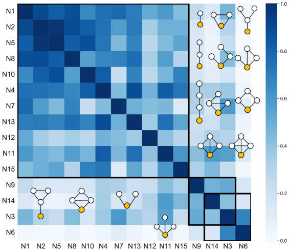
Supplementary Figure S1: The correlation matrix of 15 node orbit degrees for a contact network of high school students. Although N1, equivalent to PA, is strongly correlated with many node orbit degrees, it has relatively lower correlations to N3, N6, N9, and N14, indicating that some higher-order information, like those contained by N9 and N14, cannot be captured by the popular feature N1, or any other individual 1-order feature.

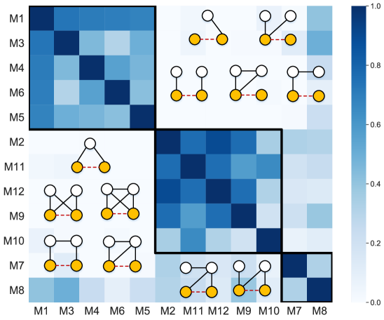
Supplementary Figure S2: The correlation matrix of 12 edge orbit degrees for a contact network of high school students. The matrix contains three clusters, emphasized by the three black boxes.

Supplementary Note 3:   Positive or negative effects of individual features

In the Fig. 3b of the main text, for a specific social network, one can observe that the feature M2 exhibits a positive effect, say a higher value of $M_{2}(x,y)$ will increase the probability that $(x,y)$ is a missing link. In contrast, the feature M4 shows a negative effect, namely a higher value of $M_{4}(x,y)$ will decrease the probability that $(x,y)$ is a missing link. In Supplementary Figure S3, we further plot the trend between the sample feature values and SHAP values. For M2, the samples with larger feature values are mostly positive samples, and their SHAP values are generally larger than 0, suggesting that the larger the M2 value of a sample, the more likely it is to be a positive sample. This is consistent with the homophily hypothesis in social networks [59], that is, the greater the number of common friends between two nodes, the higher the probability that they are friends. In contrast, for M4, samples with larger feature values are mostly negative samples, and their SHAP values are mostly less than 0. That is to say, the larger the M4 value of a sample, the more likely it is to be a negative sample. Looking closely at $M_{4}(x,y)$, a larger $M_{4}(x,y)$ is statistically associated with a larger $k_{x}$, a larger $k_{y}$, a fewer common neighbors of $x$ and $y$, and a fewer direct connections between $x$’s neighbors and $y$’s neighbors. As is well known, the formation of most real-world networks adheres to a crucial principle known as the locality principle. Link prediction algorithms based on 2-hop paths (i.e., common neighbors) [17, 19], 3-hop paths [12, 83, 52] and local community paradigm [51], all rely on this principle. Since the last two factors related to larger values of $M_{4}(x,y)$ are contrary to the locality principle, a larger $M_{4}(x,y)$ will statistically decrease the likelihood of a link connecting $x$ and $y$.

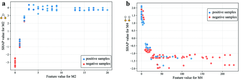
Supplementary Figure S3: The relationship between sample feature values and SHAP values. Each point represents a sample, with blue indicating positive samples and orange indicating negative samples.

Supplementary Note 4:   Analyzing transportation sub-domain

Similar to Fig. 4c of the main text, we show the winning rates of features for networks in different transportation sub-domains. As shown in Supplementary Figure S4, the first-ranked features in different sub-domains (i.e., airports, public transports and roads) are largely different, illustrating the more complex formation mechanisms of transportation networks than social networks that are dominated by the homophily mechanism.

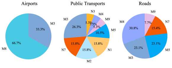
Supplementary Figure S4: The winning rates subject to the highest mean absolute SHAP values of all features in sub-domains of transportation networks.

Supplementary Note 5:   M3 and star structure

In Fig. 4b of the main text, we show that M3$(\vbox{\hbox{\includegraphics[width=12.05553pt,height=12.05553pt]{./motif/M3.pdf}}})$ has the highest winning rate across economic, technological, and information networks. Obviously, in M3, the target link can be considered as a link in a star network. To have an intuitive understanding, we visualize an example economic network detailing affiliations among Norwegian public limited companies and their board directors [38]. As shown in Supplementary Figure S5, this network contains many local stars, and any link associated with a hub node in a local star will have a high $M3$ value. Therefore, the M3 predictor performs well in this network.

Supplementary Figure S5: Visualization of the example Norwegian economic network. This network exhibits rich local star-like structures, which can be well characterized by M3.

References

- [1] Réka Albert and Albert-László Barabási. Statistical mechanics of complex networks. Reviews of modern physics, 74(1):47, 2002.
- [2] Mark EJ Newman. The structure and function of complex networks. SIAM review, 45(2):167–256, 2003.
- [3] Linyuan Lü and Tao Zhou. Link prediction in complex networks: A survey. Physica A, 390(6):1150–1170, 2011.
- [4] Tao Zhou. Progresses and challenges in link prediction. iScience, 24:103217, 2021.
- [5] Wen-Qiang Wang, Qian-Ming Zhang, and Tao Zhou. Evaluating network models: A likelihood analysis. Europhysics Letters, 98(2):28004, 2012.
- [6] Qian-Ming Zhang, Xiao-Ke Xu, Yu-Xiao Zhu, and Tao Zhou. Measuring multiple evolution mechanisms of complex networks. Scientific Reports, 5(1):10350, 2015.
- [7] Toni Vallès-Català, Tiago P Peixoto, Marta Sales-Pardo, and Roger Guimerà. Consistencies and inconsistencies between model selection and link prediction in networks. Physical Review E, 97(6):062316, 2018.
- [8] Amir Ghasemian, Homa Hosseinmardi, and Aaron Clauset. Evaluating overfit and underfit in models of network community structure. IEEE Transactions Knowledge and Data Engineering, 32(9):1722–1735, 2019.
- [9] Luca Maria Aiello, Alain Barrat, Rossano Schifanella, Ciro Cattuto, Benjamin Markines, and Filippo Menczer. Friendship prediction and homophily in social media. ACM Transactions the Web, 6(2):9, 2012.
- [10] Linyuan Lü, Matúš Medo, Chi Ho Yeung, Yi-Cheng Zhang, Zi-Ke Zhang, and Tao Zhou. Recommender systems. Physics Reports, 519(1):1–49, 2012.
- [11] Aaron Clauset, Cristopher Moore, and Mark EJ Newman. Hierarchical structure and the prediction of missing links in networks. Nature, 453(7191):98–101, 2008.
- [12] István A Kovács, Katja Luck, Kerstin Spirohn, Yang Wang, Carl Pollis, Sadie Schlabach, Wenting Bian, Dae-Kyum Kim, Nishka Kishore, Tong Hao, et al. Network-based prediction of protein interactions. Nature Communications, 10:1240, 2019.
- [13] Zhuo-Ming Ren, An Zeng, and Yi-Cheng Zhang. Structure-oriented prediction in complex networks. Physics Reports, 750:1–51, 2018.
- [14] Ajay Kumar, Shashank Sheshar Singh, Kuldeep Singh, and Bhaskar Biswas. Link prediction techniques, applications, and performance: A survey. Physica A: Statistical Mechanics and its Applications, 553:124289, 2020.
- [15] Yijun Ran, Xiao-Ke Xu, and Tao Jia. The maximum capability of a topological feature in link prediction. PNAS nexus, 3(3):pgae113, 2024.
- [16] Albert-László Barabási and Réka Albert. Emergence of scaling in random networks. Science, 286(5439):509–512, 1999.
- [17] David Liben-Nowell and Jon Kleinberg. The link-prediction problem for social networks. Journal of the American Society Information Science and Technology, 58(7):1019–1031, 2007.
- [18] Fragkiskos Papadopoulos, Maksim Kitsak, M Ángeles Serrano, Marián Boguná, and Dmitri Krioukov. Popularity versus similarity in growing networks. Nature, 489(7417):537–540, 2012.
- [19] Tao Zhou, Linyuan Lü, and Yi-Cheng Zhang. Predicting missing links via local information. European Physical Journal B, 71(4):623–630, 2009.
- [20] Linyuan Lü, Ci-Hang Jin, and Tao Zhou. Similarity index based on local paths for link prediction of complex networks. Physical Review E, 80(4):046122, 2009.
- [21] Ron Milo, Shai Shen-Orr, Shalev Itzkovitz, Nadav Kashtan, Dmitri Chklovskii, and Uri Alon. Network motifs: simple building blocks of complex networks. Science, 298(5594):824–827, 2002.
- [22] Qian-Ming Zhang, Linyuan Lü, Wen-Qiang Wang, Yu-Xiao Zhu, and Tao Zhou. Potential theory for directed networks. PLoS ONE, 8(2):e55437, 2013.
- [23] Feng Xia, Haoran Wei, Shuo Yu, Da Zhang, and Bo Xu. A survey of measures for network motifs. IEEE Access, 7:106576–106587, 2019.
- [24] Si-Yuan Liu, Jing Xiao, and Xiao-Ke Xu. Link prediction in signed social networks: From status theory to motif families. IEEE Transactions Network Science and Engineering, 7(3):1724–1735, 2019.
- [25] Yafang Liu, Ting Li, and Xiaoke Xu. Link prediction by multiple motifs in directed networks. IEEE Access, 8:174–183, 2019.
- [26] Lei Wang, Jing Ren, Bo Xu, Jianxin Li, Wei Luo, and Feng Xia. Model: Motif-based deep feature learning for link prediction. IEEE Transactions Computational Social Systems, 7(2):503–516, 2020.
- [27] Chao Li, Wei Wei, Xiangnan Feng, and Jiaomin Liu. Research of motif-based similarity for link prediction problem. IEEE Access, 9:66636–66645, 2021.
- [28] Feng Xia, Shuo Yu, Chengfei Liu, Jianxin Li, and Ivan Lee. Chief: clustering with higher-order motifs in big networks. IEEE Transactions Network Science and Engineering, 9(3):990–1005, 2021.
- [29] Bryan Perozzi, Rami Al-Rfou, and Steven Skiena. Deepwalk: Online learning of social representations. In Proceedings of the 20th ACM SIGKDD International Conference on Knowledge Discovery and Data Mining, pages 701–710. ACM Press, 2014.
- [30] Aditya Grover and Jure Leskovec. node2vec: Scalable feature learning for networks. In Proceedings of the 22nd ACM SIGKDD International Conference on Knowledge Discovery and Data Mining, pages 855–864. ACM Press, 2016.
- [31] Ren-Meng Cao, Si-Yuan Liu, and Xiao-Ke Xu. Network embedding for link prediction: The pitfall and improvement. Chaos, 29:103102, 2019.
- [32] Alexandru Cristian Mara, Jefrey Lijffijt, and Tijl de Bie. Benchmarking network embedding models for link prediction: are we making progress? In 2020 IEEE 7th International Conference on Data Science and Advanced Analytics (DSAA), pages 138–147. IEEE, 2020.
- [33] Xu-Wen Wang, Yize Chen, and Yang-Yu Liu. Link prediction through deep generative model. iScience, 23(10):101626, 2020.
- [34] Muhan Zhang and Yixin Chen. Link prediction based on graph neural networks. Advances in Neural Information Processing Systems, 31:5171–5181, 2018.
- [35] Mario Krenn, Lorenzo Buffoni, Bruno Coutinho, Sagi Eppel, Jacob Gates Foster, Andrew Gritsevskiy, Harlin Lee, Yichao Lu, João P Moutinho, Nima Sanjabi, et al. Forecasting the future of artificial intelligence with machine learning-based link prediction in an exponentially growing knowledge network. Nature Machine Intelligence, 5(11):1326–1335, 2023.
- [36] Alessandro Muscoloni and Carlo Vittorio Cannistraci. “stealing fire or stacking knowledge” by machine intelligence to model link prediction in complex networks. iScience, 26(1):105687, 2023.
- [37] Nicolas Menand and C Seshadhri. Link prediction using low-dimensional node embeddings: The measurement problem. Proceedings of the National Academy of Sciences USA, 121(8):e2312527121, 2024.
- [38] Amir Ghasemian, Homa Hosseinmardi, Aram Galstyan, Edoardo M Airoldi, and Aaron Clauset. Stacking models for nearly optimal link prediction in complex networks. Proceedings of the National Academy of Sciences USA, 117(38):23393–23400, 2020.
- [39] Natasa Pržulj, Derek G Corneil, and Igor Jurisica. Modeling interactome: scale-free or geometric? Bioinformatics, 20(18):3508–3515, 2004.
- [40] Nataša Pržulj. Biological network comparison using graphlet degree distribution. Bioinformatics, 23(2):e177–e183, 2007.
- [41] A Vazquez, R Dobrin, D Sergi, J-P Eckmann, Zoltan N Oltvai, and A-L Barabási. The topological relationship between the large-scale attributes and local interaction patterns of complex networks. Proceedings of the National Academy of Sciences USA, 101(52):17940–17945, 2004.
- [42] Kai-Yang Chiang, Nagarajan Natarajan, Ambuj Tewari, and Inderjit S Dhillon. Exploiting longer cycles for link prediction in signed networks. In Proceedings of the 20th ACM International Conference on Information and Knowledge Management, pages 1157–1162. ACM Press, 2011.
- [43] Lars Backstrom and Jon Kleinberg. Romantic partnerships and the dispersion of social ties: a network analysis of relationship status on facebook. In Proceedings of the 17th ACM conference on Computer supported cooperative work & social computing, pages 831–841. ACM Press, 2014.
- [44] Yuxiao Dong, Reid A Johnson, Jian Xu, and Nitesh V Chawla. Structural diversity and homophily: A study across more than one hundred big networks. In Proceedings of the 23rd ACM SIGKDD International Conference on Knowledge Discovery and Data Mining, pages 807–816. ACM Press, 2017.
- [45] Tijana Milenković and Nataša Pržulj. Uncovering biological network function via graphlet degree signatures. Cancer Informatics, 6:CIN.S680, 2008.
- [46] Yuriy Hulovatyy, Ryan W Solava, and Tijana Milenković. Revealing missing parts of the interactome via link prediction. PLoS ONE, 9(3):e90073, 2014.
- [47] Jian Feng and Shaojian Chen. Link prediction based on orbit counting and graph auto-encoder. IEEE Access, 8:226773–226783, 2020.
- [48] Ryan W Solava, Ryan P Michaels, and Tijana Milenković. Graphlet-based edge clustering reveals pathogen-interacting proteins. Bioinformatics, 28(18):i480–i486, 2012.
- [49] Julie Fournet and Alain Barrat. Contact patterns among high school students. PLoS ONE, 9(9):e107878, 2014.
- [50] Lada A Adamic and Eytan Adar. Friends and neighbors on the web. Social Networks, 25(3):211–230, 2003.
- [51] Carlo Vittorio Cannistraci, Gregorio Alanis-Lobato, and Timothy Ravasi. From link-prediction in brain connectomes and protein interactomes to the local-community-paradigm in complex networks. Scientific Reports, 3(1):1613, 2013.
- [52] Tao Zhou, Yan-Li Lee, and Guannan Wang. Experimental analyses on 2-hop-based and 3-hop-based link prediction algorithms. Physica A, 564:125532, 2021.
- [53] Yoav Goldberg and Omer Levy. word2vec explained: deriving mikolov et al.’s negative-sampling word-embedding method. arXiv:1402.3722, 2014.
- [54] Zhen Yang, Ming Ding, Chang Zhou, Hongxia Yang, Jingren Zhou, and Jie Tang. Understanding negative sampling in graph representation learning. In Proceedings of the 26th ACM SIGKDD international conference on knowledge discovery & data mining, pages 1666–1676. ACM Press, 2020.
- [55] Tianqi Chen and Carlos Guestrin. Xgboost: A scalable tree boosting system. In Proceedings of the 22nd ACM SIGKDD International Conference on Knowledge Discovery and Data Mining, pages 785–794. ACM Press, 2016.
- [56] Weihua Lei, Luiz GA Alves, and Luís A Nunes Amaral. Forecasting the evolution of fast-changing transportation networks using machine learning. Nature Communications, 13(1):4252, 2022.
- [57] Leo Katz. A new status index derived from sociometric analysis. Psychometrika, 18(1):39–43, 1953.
- [58] Claire Donnat, Marinka Zitnik, David Hallac, and Jure Leskovec. Learning structural node embeddings via diffusion wavelets. In Proceedings of the 24th ACM SIGKDD International Conference on Knowledge Discovery & Data Mining, pages 1320–1329. ACM Press, 2018.
- [59] Miller McPherson, Lynn Smith-Lovin, and James M Cook. Birds of a feather: Homophily in social networks. Annual Review of Sociology, 27(1):415–444, 2001.
- [60] Mark E J Newman and Juyong Park. Why social networks are different from other types of networks. Physical Review E, 68(3):036122, 2003.
- [61] Ernesto Estrada. Topological structural classes of complex networks. Physical Review E, 75(1):016103, 2007.
- [62] Harold Hotelling. Analysis of a complex of statistical variables into principal components. Journal of Educational Psychology, 24(6):417–441, 1933.
- [63] Alain Barrat, Marc Barthelemy, Romualdo Pastor-Satorras, and Alessandro Vespignani. The architecture of complex weighted networks. Proceedings of the National Academy of Sciences USA, 101(11):3747–3752, 2004.
- [64] Diego Garlaschelli and Maria I Loffredo. Patterns of link reciprocity in directed networks. Physical Review Letters, 93(26):268701, 2004.
- [65] Petter Holme and Jari Saramäki. Temporal networks. Physics Reports, 519(3):97–125, 2012.
- [66] Marc Barthélemy. Spatial networks. Physics Reports, 499(1-3):1–101, 2011.
- [67] Christian Bick, Elizabeth Gross, Heather A Harrington, and Michael T Schaub. What are higher-order networks? SIAM Review, 65(3):686–731, 2023.
- [68] Austin R Benson, Rediet Abebe, Michael T Schaub, Ali Jadbabaie, and Jon Kleinberg. Simplicial closure and higher-order link prediction. Proceedings of the National Academy of Sciences USA, 115(48):E11221–E11230, 2018.
- [69] Iacopo Iacopini, Giovanni Petri, Alain Barrat, and Vito Latora. Simplicial models of social contagion. Nature Communications, 10(1):2485, 2019.
- [70] James A Hanley and Barbara J McNeil. The meaning and use of the area under a receiver operating characteristic (roc) curve. Radiology, 143(1):29–36, 1982.
- [71] Andrew P Bradley. The use of the area under the roc curve in the evaluation of machine learning algorithms. Pattern recognition, 30(7):1145–1159, 1997.
- [72] Tao Zhou. Discriminating abilities of threshold-free evaluation metrics in link prediction. Physica A: Statistical Mechanics and its Applications, 615:128529, 2023.
- [73] Xinshan Jiao, Shuyan Wan, Qian Liu, Yilin Bi, Yan-Li Lee, En Xu, Dong Hao, and Tao Zhou. Comparing discriminating abilities of evaluation metrics in link prediction. Journal of Physics: Complexity, 5:025014, 2024.
- [74] Yang Yang, Ryan N Lichtenwalter, and Nitesh V Chawla. Evaluating link prediction methods. Knowledge and Information Systems, 45:751–782, 2015.
- [75] Takaya Saito and Marc Rehmsmeier. The precision-recall plot is more informative than the roc plot when evaluating binary classifiers on imbalanced datasets. PLoS ONE, 10(3):e0118432, 2015.
- [76] Michael Buckland and Fredric Gey. The relationship between precision and recall. Journal of the American Society for Information Science, 45(1):12–19, 1994.
- [77] Yutaka Sasaki et al. The truth of the f-measure. Teach Tutor Mater, 1(5):1–5, 2007.
- [78] Yilin Bi, Xinshan Jiao, Yan-Li Lee, and Tao Zhou. Inconsistency of evaluation metrics in link prediction. arXiv:2402.08893, 2024.
- [79] Lloyd S Shapley. A value for n-person games. Annals of Mathematics Studies, 28:307–318, 1953.
- [80] Scott M Lundberg and Su-In Lee. A unified approach to interpreting model predictions. In Proceedings of the 31st International Conference on Neural Information Processing Systems, pages 4768–4777. NeurIPS, 2017.
- [81] Yuan Meng, Nianhua Yang, Zhilin Qian, and Gaoyu Zhang. What makes an online review more helpful: an interpretation framework using xgboost and shap values. Journal of Theoretical and Applied Electronic Commerce Research, 16(3):466–490, 2021.
- [82] Manfred Mudelsee. Estimating pearson’s correlation coefficient with bootstrap confidence interval from serially dependent time series. Mathematical Geology, 35:651–665, 2003.
- [83] Ratha Pech, Dong Hao, Yan-Li Lee, Ye Yuan, and Tao Zhou. Link prediction via linear optimization. Physica A, 528:121319, 2019.