Zak-OTFS with Interleaved Pilots to Extend the Region of Predictable Operation

Abstract

When the delay period of the Zak-OTFS carrier is greater than the delay spread of the channel, and the Doppler period of the carrier is greater than the Doppler spread of the channel, the effective channel filter taps can simply be read off from the response to a single pilot carrier waveform. The input-output (I/O) relation can then be reconstructed for a sampled system that operates under finite duration and bandwidth constraints. We introduce a framework for pilot design in the delay-Doppler (DD) domain which makes it possible to support users with very different delay-Doppler characteristics when it is not possible to choose a single delay and Doppler period to support all users. The method is to interleave single pilots in the DD domain, and to choose the pilot spacing so that the I/O relation can be reconstructed by solving a small linear system of equations.

I Introduction

The Zak-OTFS carrier waveform is a pulse in the delay-Doppler(DD) domain, that is a quasi-periodic localized function defined by a delay period $\tau_{p}$ and a Doppler period $\nu_{p}$ where $\tau_{p}\,\nu_{p}=1$. The time-domain (TD) realization of the carrier is a pulsone, that is a train of pulses modulated by a tone where adjacent pulses are spaced $\tau_{p}$ seconds apart. The frequency-domain (FD) realization of the carrier is a train of pulses in the frequency domain (FD) modulated by a FD sinusoid where adjacent pulses are spaced $\nu_{p}$ Hz apart. We have shown [1] that the Zak-OTFS input-output (I/O) relation is predictable and non-fading when the delay period of the pulsone is greater than the delay spread of the channel and the Doppler period of the pulsone is greater than the Doppler spread of the channel. We refer to this condition as the crystallization condition. When the crystallization condition holds, the taps of the effective DD domain channel filter can simply be read off from the DD domain response to a single pilot carrier waveform, and the I/O relation can be reconstructed for a sampled system that operates under finite duration and bandwidth constraints. Section II describes the Zak-OTFS system model.

4G and 5G wireless communication networks use OFDM rather than Zak-OTFS. However OFDM exhibits poor reliability for high delay and Doppler spreads characteristic of next generation communication scenarios [2], [3, 4, 6]. The first instantiation of OTFS was designed to be compatible with 4G/5G modems and is called MC-OTFS (Multicarrier OTFS). MC-OTFS is superior to OFDM for high delay and Doppler spreads [7, 8], but is inferior to Zak-OTFS [1]. Note that in MC-OTFS, modulation, detection and estimation are all performed in the DD domain [9, 10, 11, 12]. The OTFS Special Interest Group (SIG) website [13] is a rich source of information about MC-OTFS.

In MC-OTFS, DD domain information symbols are transformed to time-frequency (TF) symbols which are then used to generate the transmitted TD signal. This two-step modulation can be avoided by using the Zak-transform [14, 15] to obtain the transmitted TD signal directly from the DD domain information symbols (see [16, 17] for details). This method of modulation is called Zak-OTFS (see [18, 1] for details) and it achieves better throughput/reliability than MC-OTFS, particularly in high delay/Doppler spread scenarios. There are also implementations based on the discrete Zak transform [19] and on TF windowing [20]. Filtering in the discrete DD domain generate noise-like pilot waveforms (spread pilots) that enable integrated sensing and communication (ISAC) in the same Zak-OTFS subframe [21].

We emphasize that we are learning the I/O relation without estimating the physical channel parameters (gain, delay and Doppler shift of each physical path). By focusing not on acquiring the channel, but on acquiring the interaction of channel and modulation, Zak-OTFS circumvents the legacy channel model dependent approach to wireless communications and operates model-free. We present numerical simulations in Section VI for the Veh-A channel model [22] which consists of six channel paths and is representative of real propagation environments. In these simulations, we deliberately choose the channel bandwidth so that not all paths are separable/resolvable, and it is not possible to estimate the physical channel.

Why Zak-OTFS rather than OFDM? Perhaps the most important reason is that 6G propagation environments are changing the balance between time-frequency methods focused on OFDM signal processing and delay-Doppler (DD) methods focused on Zak-OTFS signal processing. OFDM signals live on a coarse information grid (i.e., integer multiples of the sub-carrier spacing), and cyclic prefix/carrier spacing are designed to prevent inter carrier interference (ICI). When there is no ICI, equalization in OFDM is relatively simple once the I/O relation is acquired. However, acquisition of the Input/Output (I/O) relation in OFDM is non-trivial and model-dependent, and the interaction of the OFDM carrier with the channel varies in both TD and FD. By contrast Zak-OTFS signals live on a fine information grid. Since information carrying DD pulses are located on a finer grid, they interfere with each other resulting in inter-carrier interference due to which equalization is more involved. However, when the crystallization condition holds the I/O relation can be read off from the response to a single pilot signal. In this paper we focus on acquiring the I/O relation.

We consider the challenge of supporting two types of user with very different delay-Doppler characteristics without changing the delay and Doppler periods of the Zak-OTFS modulation. For simplicity, we focus on supporting a second user with delay spread $\tau_{max}$ at most $\tau_{p}/2$ and Doppler spread $2\nu_{max}$ satisfying $\nu_{p}<2\nu_{max}<2\nu_{p}$. We would be able to support this user by halving the delay period and doubling the Doppler period, but then we cannot choose a single delay and Doppler period to support both users.

Section III describes how to place two interleaved pilots on the original Zak-OTFS grid so that the I/O relation for the second user can be obtained by solving a $2\times 2$ linear system. The method is simple and effective, but it is not the maximum likelihood (ML) estimate. In Section V, we analyze the ML estimator which is given by the samples of the cross-ambiguity between the received DD domain interleaved pilot and the transmitted DD domain interleaved pilot. The cross-ambiguity function is supported on a rectangular lattice in the DD domain, and the effective channel taps can be read off by restricting to any fundamental domain of this lattice. The delay and Doppler spacing of this lattice determine a second effective crystallization condition and interleaved pilots make it possible to support users that satisfy either of the two crystallization conditions on a system with a single delay period and single Doppler period.

In Section VI we simulate the bit error rate (BER) performance of a Zak-OTFS subframe with interleaved pilots. For a fixed data signal power to noise power ratio (SNR) and fixed pilot power to data power ratio (PDR), it is observed that with every doubling in the number of interleaved pilots the maximum Doppler spread for which reliable/predictable operation is achieved, is also roughly doubled, i.e., extension in the region of predictable operation. Also, the peak to average power ratio (PAPR) of the transmit TD signal reduces by $3$ dB for every doubling in the number of interleaved pilots.

II System model

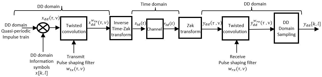
Figure 1: Zak-OTFS transceiver processing.

Zak-OTFS transceiver processing is illustrated in Fig. 1 (see Section II of [1] also). We transmit $MN$ symbols $x[k_{0},l_{0}]$ in each subframe, $k_{0}=0,1,\cdots,M-1$, $l_{0}=0,1,\cdots,N-1$. The discrete DD domain pulse $x_{\mbox{\scriptsize{dd}}}^{(k_{0},l_{0})}[k,l]$ carries the information symbol $x[k_{0},l_{0}]$, i.e.

$$x_{\mbox{\scriptsize{dd}}}^{(k_{0},l_{0})}[k,l] = \sum\limits_{n,m\in{\mathbb{Z}}}{\Big{(}}e^{j2\pi\frac{nl_{0}}{N}}\,x[k_{0},l_{0}]\,\delta[k-k_{0}-nM]$$ (1)

$$\hskip 28.45274pt\delta[l-l_{0}-mN]{\Big{)}},$$

for all $k,l\in{\mathbb{Z}}$. From (1) it is clear that this pulse carrying the $(k_{0},l_{0})$-th information symbol consists of infinitely many Dirac-delta impulses at discrete DD locations $(k_{0}+nM,l_{0}+mN)$, $n,m\in{\mathbb{Z}}$. Also, irrespective of $(k_{0},l_{0})$, $x_{\mbox{\scriptsize{dd}}}^{(k_{0},l_{0})}[k,l]$ is a quasi-periodic function with period $M$ along the delay axis and period $N$ along the Doppler axis, i.e., for any $n,m\in{\mathbb{Z}}$, $x_{\mbox{\scriptsize{dd}}}^{(k_{0},l_{0})}[k,l]$ satisfies

$$x_{\mbox{\scriptsize{dd}}}^{(k_{0},l_{0})}[k+nM,l+mN] = e^{j2\pi\frac{nl_{0}}{N}}\,x_{\mbox{\scriptsize{dd}}}^{(k_{0},l_{0})}[k,l].$$ (2)

The discrete DD domain pulses corresponding to all $MN$ information symbols are superimposed resulting in the discrete quasi-periodic DD domain signal

$$x_{\mbox{\scriptsize{dd}}}[k,l] = \sum\limits_{k_{0}=0}^{M-1}\sum\limits_{l_{0}=0}^{N-1}x_{\mbox{\scriptsize{dd}}}^{(k_{0},l_{0})}[k,l].$$ (3)

$x_{\mbox{\scriptsize{dd}}}[k,l]$ is supported on the information lattice $\Lambda_{dd}=\{\left(\frac{k\tau_{p}}{M},\frac{l\nu_{p}}{N}\right)\,|\,k,l\in{\mathbb{Z}}\}$, i.e., we lift the discrete signal $x_{\mbox{\scriptsize{dd}}}[k,l]$ to the continuous DD domain signal

$$x_{\mbox{\scriptsize{dd}}}(\tau,\nu) = \sum\limits_{k,l\in{\mathbb{Z}}}x_{\mbox{\scriptsize{dd}}}[k,l]\,\delta\left(\tau-\frac{k\tau_{p}}{M}\right)\,\delta\left(\nu-\frac{l\nu_{p}}{N}\right).$$ (4)

Note that, for any $n,m\in{\mathbb{Z}}$

$$x_{\mbox{\scriptsize{dd}}}(\tau+n\tau_{p},\nu+m\nu_{p}) = e^{j2\pi n\nu\tau_{p}}\,x_{\mbox{\scriptsize{dd}}}(\tau,\nu),$$ (5)

so that $x_{\mbox{\scriptsize{dd}}}(\tau,\nu)$ is periodic with period $\nu_{p}$ along the Doppler axis and quasi-periodic with period $\tau_{p}$ along the delay axis.

We use a pulse shaping filter $w_{tx}(\tau,\nu)$ to limit the TD Zak-OTFS subframe to time duration $T=N\tau_{p}$ and bandwidth $B=M\nu_{p}$. The DD domain transmit signal $x_{\mbox{\scriptsize{dd}}}^{w_{tx}}(\tau,\nu)$ is given by the twisted convolution of the transmit pulse shaping filter $w_{tx}(\tau,\nu)$ with $x_{\mbox{\scriptsize{dd}}}(\tau,\nu)$.

$$x_{\mbox{\scriptsize{dd}}}^{w_{tx}}(\tau,\nu) = w_{tx}(\tau,\nu)\,*_{\sigma}\,x_{\mbox{\scriptsize{dd}}}(\tau,\nu),$$ (6)

where $*_{\sigma}$ denotes the twisted convolution operator [18, 1]. The TD realization of $x_{\mbox{\scriptsize{dd}}}^{w_{tx}}(\tau,\nu)$ gives the transmitted TD signal which is given by

$$s_{\mbox{\scriptsize{td}}}(t) = {\mathcal{Z}}_{t}^{-1}\left(x_{\mbox{\scriptsize{dd}}}^{w_{tx}}(\tau,\nu)\right),$$ (7)

where ${\mathcal{Z}}_{t}^{-1}$ denotes the inverse Zak transform (see Eqn. $(7)$ in [18] for more details).

The received TD signal is given by

$$r_{\mbox{\scriptsize{td}}}(t) = \iint h_{\mbox{\scriptsize{phy}}}(\tau,\nu)\,s_{\mbox{\scriptsize{td}}}(t-\tau)\,e^{j2\pi\nu(t-\tau)}\,d\tau\,d\nu\,+\,n_{\mbox{\scriptsize{td}}}(t),$$

where $h_{\mbox{\scriptsize{phy}}}(\tau,\nu)$ is the delay-Doppler spreading function of the physical channel and $n_{\mbox{\scriptsize{td}}}(t)$ is AWGN. At the receiver, we pass from the TD to the DD domain by applying the Zak transform ${\mathcal{Z}}_{t}$ to the received TD signal $r_{\mbox{\scriptsize{td}}}(t)$, and we obtain

$$y_{\mbox{\scriptsize{dd}}}(\tau,\nu) = {\mathcal{Z}}_{t}\left(r_{\mbox{\scriptsize{td}}}(t)\right).$$ (9)

Substituting (II) into (9) it follows that [18, 1]

$$y_{\mbox{\scriptsize{dd}}}(\tau,\nu) = h_{\mbox{\scriptsize{phy}}}(\tau,\nu)\,*_{\sigma}\,x_{\mbox{\scriptsize{dd}}}^{w_{tx}}(\tau,\nu)\,+\,n_{\mbox{\scriptsize{dd}}}(\tau,\nu),$$ (10)

where $n_{\mbox{\scriptsize{dd}}}(\tau,\nu)$ is the DD representation of the AWGN. Note that, in the DD domain the channel acts on the input $x_{\mbox{\scriptsize{dd}}}^{w_{tx}}(\tau,\nu)$ through twisted convolution with $h_{\mbox{\scriptsize{phy}}}(\tau,\nu)$. This is similar to how in linear time invariant (LTI) channels (i.e., delay-only channels), the channel acts on a TD input through linear convolution with the TD channel impulse response. Twisted convolution is the generalization of linear convolution for doubly-spread channels.

Next, we apply a matched filter $w_{rx}(\tau,\nu)$ which acts by twisted convolution on $y_{\mbox{\scriptsize{dd}}}(\tau,\nu)$ to give

$$y_{\mbox{\scriptsize{dd}}}^{w_{rx}}(\tau,\nu) = w_{rx}(\tau,\nu)*_{\sigma}y_{\mbox{\scriptsize{dd}}}(\tau,\nu).$$ (11)

This filtered signal is then sampled on the information lattice $\Lambda_{\mbox{\scriptsize{dd}}}$ resulting in the quasi-periodic discrete DD domain signal $y_{\mbox{\scriptsize{dd}}}[k,l]$. This discrete DD output signal is related to the input discrete DD signal $x_{\mbox{\scriptsize{dd}}}[k,l]$ through the input-output (I/O) relation [18, 1]

$$y_{\mbox{\scriptsize{dd}}}[k,l] = h_{\mbox{\scriptsize{eff}}}[k,l]\,*_{\sigma}\,x_{\mbox{\scriptsize{dd}}}[k,l]\,+\,n_{\mbox{\scriptsize{dd}}}[k,l],$$ (12)

where $h_{\mbox{\scriptsize{eff}}}[k,l]$ is the effective DD domain channel filter and $n_{\mbox{\scriptsize{dd}}}[k,l]$ are the DD domain noise samples. Note that if $h_{\mbox{\scriptsize{eff}}}k,l]$ is simply

$$h_{\mbox{\scriptsize{eff}}}(\tau,\nu)=w_{rx}(\tau,\nu)*_{\sigma}h_{\mbox{\scriptsize{phy}}}(\tau,\nu)*_{\sigma}w_{tx}(\tau,\nu)$$ (13)

sampled on the information lattice $\Lambda_{\mbox{\scriptsize{dd}}}$, i.e.

$$h_{\mbox{\scriptsize{eff}}}[k,l] \stackrel{{\scriptstyle\Delta}}{{=}} h_{\mbox{\scriptsize{eff}}}{\Big{(}}\tau=\frac{k\tau_{p}}{M},\nu=\frac{l\nu_{p}}{N}{\Big{)}}.$$ (14)

From the I/O relation in (12) it is clear that for detecting the DD domain information symbols from $y_{\mbox{\scriptsize{dd}}}[k,l]$, it suffices to have knowledge of $h_{\mbox{\scriptsize{eff}}}[k,l]$ only. The receiver does not need to acquire $h_{\mbox{\scriptsize{phy}}}(\tau,\nu)$. Instead it acquires $h_{\mbox{\scriptsize{eff}}}[k,l]$ directly from the channel response to pilots in the discrete DD domain. This makes the Zak-OTFS I/O relation applicable to any model of the underlying physical channel and is therefore model-free. Next, we consider the acquisition of $h_{\mbox{\scriptsize{eff}}}[k,l]$.

Consider transmitting a pilot signal $x_{\mbox{\scriptsize{p,dd}}}[k,l]$ together with a data signal $x_{\mbox{\scriptsize{d,dd}}}[k,l]$ within a single Zak-OTFS subframe. Each signal is quasi-periodic, hence is completely specified by the values it takes within the fundamental region ${\mathcal{D}}=\{(k,l)\,|\,k=0,1,\cdots,M-1,l=0,1,\cdots,N-1\}$. The pilot signal $x_{\mbox{\scriptsize{p,dd}}}[k,l]$ is determined by a unit energy Dirac-delta impulse at the pilot location $(k_{p},l_{p})\in{\mathcal{D}}$ and repeats along the delay and Doppler axis by integer multiples of the delay and Doppler period respectively. It is given by

$$x_{\mbox{\scriptsize{p,dd}}}[k,l] = \sum\limits_{n,m\in{\mathbb{Z}}}e^{j2\pi n\frac{l_{p}}{N}}\,\delta[k-k_{p}-nM]\,\delta[l-l_{p}-mN].$$

The data signal $x_{\mbox{\scriptsize{d,dd}}}[k,l]$ is determined by the unit energy information symbols $x[k_{0},l_{0}]$ (${\mathbb{E}}\left[|x[k_{0},l_{0}]|^{2}\right]=1$) at locations $(k_{0},l_{0})\in{\mathcal{I}}$, where ${\mathcal{I}}\subset{\mathcal{D}}$, and is given by

$$x_{\mbox{\scriptsize{d,dd}}}[k,l] = \sum\limits_{n,m\in{\mathbb{Z}}}\sum\limits_{(k_{0},l_{0})\in{\mathcal{I}}}{\Bigg{(}}x[k_{0},l_{0}]\,e^{j2\pi\frac{l_{0}}{N}}\,\delta[k-k_{0}-nM]\,$$ (16)

$$\hskip 99.58464pt\delta[l-l_{0}-mN]{\Bigg{)}}.$$

The transmit DD domain signal is

$$x_{\mbox{\scriptsize{dd}}}[k,l] = \sqrt{\frac{E_{d}}{|{\mathcal{I}}|}}\,x_{\mbox{\scriptsize{d,dd}}}[k,l]\,+\,\sqrt{E_{p}}x_{\mbox{\scriptsize{p,dd}}}[k,l].$$ (17)

The data signal has energy $\sum\limits_{k=0}^{M-1}\sum\limits_{l=0}^{N-1}\left|\sqrt{\frac{E_{d}}{|{\mathcal{I}}|}}\,x_{\mbox{\scriptsize{d,dd}}}[k,l]\right|^{2}=E_{d}$ and the pilot signal has energy $E_{p}$. The ratio $E_{p}/E_{d}$ is the ratio of pilot power to data power (PDR).

For simplicity, we first consider channel estimation in the absence of interference from data, and we let ${\mathcal{S}}$ denote the support of the effective channel $h_{\mbox{\scriptsize{eff}}}[k,l]$. From (12) and (II), the received pilot is given by

$$h_{\mbox{\scriptsize{eff}}}[k,l]*_{\sigma}\left(\sqrt{E_{p}}\,x_{\mbox{\scriptsize{p,dd}}}[k,l]\right) = \sqrt{E_{p}}\sum\limits_{n,m\in{\mathbb{Z}}}h_{n,m}[k,l].$$ (18)

The $(n,m)$-th term $h_{n,m}[k,l]$ is the channel response to the Dirac-delta impulse of the quasi-periodic pilot signal $x_{\mbox{\scriptsize{p,dd}}}[k,l]$ located at $(k_{p}+nM,l_{p}+mN)$, and is given by

$$h_{\mbox{\scriptsize{eff}}}[k,l]*_{\sigma}\,\left(e^{j2\pi n\frac{l_{p}}{N}}\delta[k-k_{p}-nM]\,\delta[l-l_{p}-mN]\right)$$ (19)

$$={\Big{(}}h_{\mbox{\scriptsize{eff}}}[k-k_{p}-nM,l-l_{p}-mN]\,e^{j2\pi\frac{nl_{p}}{N}}$$

$$\,e^{j2\pi\frac{(l-l_{p}-mN)(k_{p}+nM)}{MN}}{\Big{)}}.$$

The support ${\mathcal{S}}_{n,m}$ of $h_{n,m}[k,l]$ is ${\mathcal{S}}+(k_{p}+nM,l_{p}+mN)$. The crystallization condition is ${\mathcal{S}}_{n,m}\cap{\mathcal{S}}_{n^{\prime},m^{\prime}}=\phi$ for $(n,m)\neq(n^{\prime},m^{\prime})$, and when it is satisfied, there is no DD domain aliasing. We have emphasized in [1] that the crystallization condition is satisfied when

$$k_{max}\stackrel{{\scriptstyle\Delta}}{{=}}\left\lceil\frac{M\tau_{max}}{\tau_{p}}\right\rceil < M,$$

$$l_{max}\stackrel{{\scriptstyle\Delta}}{{=}}\left\lceil\frac{2N\nu_{max}}{\nu_{p}}\right\rceil < N.$$ (20)

Here $\tau_{max}>0$ and $\nu_{max}>0$ are respectively the maximum possible delay and Doppler shift induced by any physical channel path. The first condition in (II) is that the channel delay spread $\tau_{max}$ is less than the delay period $\tau_{p}$, and the second condition is that the channel Doppler spread $2\nu_{max}$ is less than the Doppler period $\nu_{p}$. We refer the reader to [1], Section II-D for a more extensive discussion of crystallization conditions.

When the crystallization condition holds

$$h_{0,0}[k,l] = h_{\mbox{\scriptsize{eff}}}[k-k_{p},l-l_{p}]\,e^{j2\pi\frac{k_{p}(l-l_{p})}{MN}}$$ (21)

for $(k,l)\in(k_{p},l_{p})+{\mathcal{S}}$ and therefore

$$h_{\mbox{\scriptsize{eff}}}[k,l] = h_{0,0}[k+k_{p},l+l_{p}]\,e^{-j2\pi\frac{k_{p}l}{MN}}$$ (22)

for $(k,l)\in{\mathcal{S}}$. For $(k,l)\in{\mathcal{S}}+(k_{p},l_{p})$, the received pilot response (AWGN-free) is simply $h_{0,0}[k,l]$ since the support sets of $h_{n,m}[k,l]$, $n,m\in{\mathbb{Z}}$ do not overlap when the crystallization condition is satisfied. Hence, the taps of the effective channel filter can simply be read off from the received pilot response within ${\mathcal{S}}+(k_{p},l_{p})$. As a result the Zak-OTFS I/O relation in (12) is predictable, i.e., the AWGN-free channel response to any arbitrary input $x_{\mbox{\scriptsize{dd}}}[k,l]$ can be accurately predicted to be $h_{\mbox{\scriptsize{eff}}}[k,l]*_{\sigma}\,x_{\mbox{\scriptsize{dd}}}[k,l]$.

We now consider channel estimation in the presence of interference from data. We transmit a pilot at location $(k_{p},l_{p})$, and we surround it with pilot and guard regions where no data is transmitted. The pilot region ${\mathcal{P}}$ is given by

$${\mathcal{P}} = \{(k,l)\,|\,k_{p}-1\leq k\leq k_{p}+k_{max}$$ (23)

$$\hskip 28.45274ptl=0,1,\cdots,N-1\}.$$

The guard region ${\mathcal{G}}$ separates the pilot region from the data region comprising locations $(k_{0},l_{0})\in{\mathcal{I}}$. Fig. 2 shows pilot, guard and data regions as strips in the Zak-OTFS subframe that run parallel to the Doppler axis.

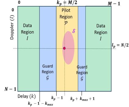
Figure 2: Zak-OTFS DD frame with single pilot (depicted by a red dot) at $(k_{p},l_{p})$. The pink shaded ellipse depicts the support set of the channel response to the pilot (i.e., ${\mathcal{S}}\,+\,(k_{p},l_{p})$).

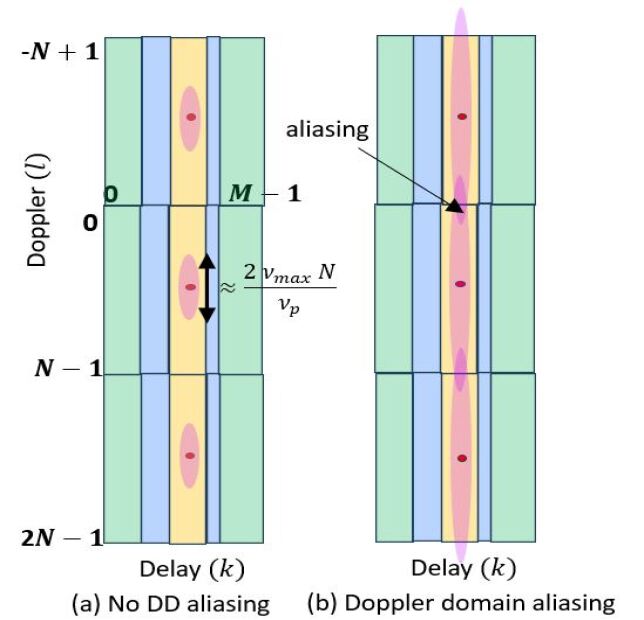
Figure 3: Doppler domain aliasing. Assuming that the channel path Doppler shift lies in $[-\nu_{max}\,,\,\nu_{max}]$, the maximum Doppler spread is $2\nu_{max}$. The Doppler resolution is $\nu_{p}/N$ (size of each Doppler bin) and the spread of the channel response is roughly $2\nu_{max}N/\nu_{p}$ bins along the Doppler axis. (a) Doppler spread is less than $N$ Doppler axis bins, and the ellipses representing the channel response to constituent pilot impulses do not overlap. (b) Doppler spread is greater than $N$ bins, and the ellipses overlap, preventing accurate estimation of the effective channel $h_{\mbox{\scriptsize{eff}}}[k,l]$.

Fig. 3 illustrates the phenomenon of Doppler domain aliasing. In Fig. $2$(b) the crystallization condition is not satisfied since the channel Doppler spread $2\nu_{max}$ is greater than the Doppler period $\nu_{p}$. In this case Doppler domain aliasing prevents accurate estimation of the effective channel $h_{\mbox{\scriptsize{eff}}}[k,l]$. One solution is to increase $\nu_{p}$ so that $\nu_{p}>2\nu_{max}$, but this changes the Zak-OTFS delay and Doppler period parameters. In this paper, we design interleaved pilots that resolve Doppler domain aliasing, thus enabling accurate estimation of the effective channel $h_{\mbox{\scriptsize{eff}}}[k,l]$ without changing the period parameters.

III Two Interleaved Pilots

For simplicity, we suppose $2\nu_{p}>2\nu_{max}\geq\nu_{p}$. We transmit two interleaved pilots at locations $(k_{p_{1}},0)$ and $(k_{p_{2}},0)$ in ${\mathcal{D}}$, and Fig. 4 illustrates how we surround each pilot with pilot and guard regions. Data is not transmitted in the pilot and guard regions. Fig. 5 illustrates the channel responses to the impulses forming the two pilots. For $i=1,2$, the response $h_{0,0}^{(i)}[k,l]$ to the impulse at $(k_{p_{i}},0)$ is shown in blue, and the response $h_{0,1}^{(i)}[k,l]$ to the impulse at $(k_{p_{i}},N)$ is shown in red. Since $2\nu_{p}>2\nu_{max}\geq\nu_{p}$, it is only the response of adjacent impulses that overlap along the Doppler axis.

For simplicity, we consider channel estimation in the absence of noise, and in the absence of interference from data. The pilot region ${\mathcal{P}}_{1}$ is given by

$${\mathcal{P}}_{1} = \{(k,l)\,|\,k_{p_{1}}-1\leq k\leq k_{p_{1}}+k_{max},$$ (24)

$$\hskip 56.9055ptl=0,1,\cdots,N-1\}.$$

It follows from (18) that the response $y_{\mbox{\scriptsize{dd}}}^{(1)}[k,l]$ to the pilot at $(k_{p_{1}},0)$, received in ${\mathcal{P}}_{1}$, is given by

$$y_{\mbox{\scriptsize{dd}}}^{(1)}[k,l] = \sqrt{\frac{E_{p}}{2}}\,h_{0,0}^{(1)}[k,l]\,+\,\sqrt{\frac{E_{p}}{2}}\,h_{0,1}^{(1)}[k,l],$$ (25)

for $(k,l)\in{\mathcal{P}}_{1}$. It now follows from (19) that for $-1\leq k\leq k_{max}$ and $l=0,1,\cdots,N-1$

$$y_{\mbox{\scriptsize{dd}}}^{(1)}[k+k_{p_{1}},l] = \sqrt{\frac{E_{p}}{2}}\,h_{\mbox{\scriptsize{eff}}}[k,l]\,e^{j2\pi\frac{lk_{p_{1}}}{MN}}$$ (26)

$$+\,\sqrt{\frac{E_{p}}{2}}\,h_{\mbox{\scriptsize{eff}}}[k,l-N]\,e^{j2\pi\frac{(l-N)k_{p_{1}}}{MN}}.$$

Note that $y_{\mbox{\scriptsize{dd}}}^{(1)}[k+k_{p_{1}},l]$ is a linear combination of the unknown taps $h_{\mbox{\scriptsize{eff}}}[k,l]$ and $h_{\mbox{\scriptsize{eff}}}[k,l-N]$. Let $y_{\mbox{\scriptsize{dd}}}^{(2)}[k,l]$ denote the response to the pilot at $(k_{p_{2}},0)$ received in the pilot region ${\mathcal{P}}_{2}$. Therefore

$$y_{\mbox{\scriptsize{dd}}}^{(2)}[k+k_{p_{2}},l] = \sqrt{\frac{E_{p}}{2}}\,h_{\mbox{\scriptsize{eff}}}[k,l]\,e^{j2\pi\frac{lk_{p_{2}}}{MN}}$$ (27)

$$+\,\sqrt{\frac{E_{p}}{2}}\,h_{\mbox{\scriptsize{eff}}}[k,l-N]\,e^{j2\pi\frac{(l-N)k_{p_{2}}}{MN}},$$

for $-1\leq k\leq k_{max}$, $l=0,1,\cdots,N-1$. When $k_{p_{1}}\neq k_{p_{2}}$ (mod $M$), equations (26) and (27) are linearly independent, and it is possible to solve for $h_{\mbox{\scriptsize{eff}}}[k,l]$ and $h_{\mbox{\scriptsize{eff}}}[k,l-N]$. When the channel Doppler spread satisfies $2\nu_{p}>2\nu_{max}\geq\nu_{p}$, the discrete Doppler domain spread is less than $2N$, and therefore the effective channel taps $h_{\mbox{\scriptsize{eff}}}[k,l]$ can be acquired accurately for all $(k,l)\in{\mathcal{S}}$. The I/O relation is predictable because it is possible to acquire the effective channel.

If the data and guard regions were not present in Fig. 4, the minimum possible delay domain pilot spacing $\min_{n_{1},n_{2}\in{\mathbb{Z}}}\left|k_{p_{2}}+n_{2}M-k_{p_{1}}-n_{1}M\right|$ should be chosen as $k_{max}+2$ in order to avoid delay domain aliasing between the response to pilots which are adjacent along the delay axis. Since pilots are quasi-periodic with delay period $M$, we have $M\geq 2(k_{max}+2)$ and therefore the delay spread $\tau_{max}$ satisfies $\tau_{max}\leq\tau_{p}/2\,-\,2\tau_{p}/M$. We define the effective delay period $\tau_{\mbox{\scriptsize{p,eff}}}=\tau_{p}/2$ and the effective Doppler period $\nu_{\mbox{\scriptsize{p,eff}}}=2\nu_{p}$, noting that the product $\tau_{\mbox{\scriptsize{p,eff}}}\,\nu_{\mbox{\scriptsize{p,eff}}}=1$ is unchanged. The I/O relation is predictable when the following effective crystallization condition is satisfied

$$k_{max}+2\leq\frac{M}{2}\,\,\mbox{\small{and}}\,\,\left\lceil\frac{2\nu_{max}N}{\nu_{p}}\right\rceil\,<\,2N.$$ (28)

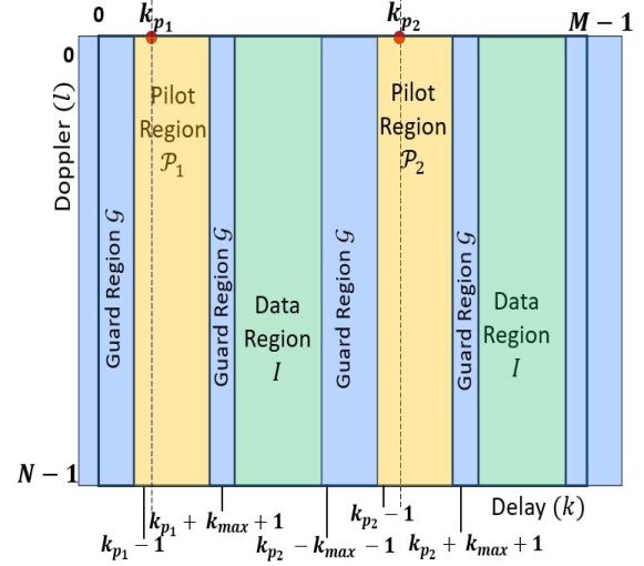
Figure 4: Zak-OTFS subframe with two interleaved pilots (indicated by red dots) at $(k_{p_{1}},0)$ and $(k_{p_{2}},0)$.

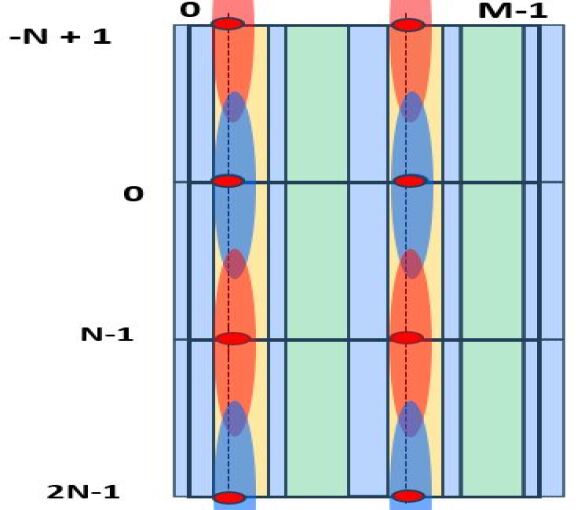
Figure 5: Doppler domain aliasing with two superimposed pilots.

Interleaved pilots make it possible to change the aspect ratio of the crystallization condition without changing the fundamental periods, $\tau_{p}$ and $\nu_{p}$. Here, we have illustrated the method of interleaved pilots for the case $2\nu_{p}>\nu_{max}\geq\nu_{p}$. By symmetry, a similar method applies to the case $2\tau_{p}>\tau_{max}\geq\tau_{p}$, with the only difference being that the pilots are interleaved along the Doppler axis and are also multiplied with distinct known unit modulus complex scalars. This is required, since the pilot is periodic along the Doppler axis and therefore without any multiplication with complex scalars the corresponding equations (26) and (27) will not be linearly independent.

IV Multiple Interleaved Pilots

The generalization to $Q$ interleaved pilots is required when $(Q-1)\nu_{p}\leq 2\nu_{max}<Q\nu_{p}$. We transmit $Q$ interleaved pilots at locations $(k_{p_{i}},0)\in{\mathcal{D}},i=1,2\cdots,Q$, separated by pilots regions ${\mathcal{P}}_{i}$ and guard regions. The response $y_{\mbox{\scriptsize{dd}}}^{(i)}[k,l]$ to the pilot $(k_{p_{i}},0)$ received in ${\mathcal{P}}_{i}$ is a linear combination of $Q$ distinct taps of $h_{\mbox{\scriptsize{eff}}}[k,l]$. The responses $y_{\mbox{\scriptsize{dd}}}^{(i)}[k,l]$, $i=1,2,\cdots,Q$, yield $Q$ linear equations in the $Q$ unknown taps, and since the pilot locations are distinct, these equations are linearly independent. We estimate the taps $h_{\mbox{\scriptsize{eff}}}[k,l]$, where $k=-1,\cdots,k_{max}$ with $l=-\frac{Q}{2}N,\cdots,0,\cdots,(\frac{Q}{2}-1)N$ if $Q$ is even, and $l=-\frac{(Q-1)}{2}N,\cdots,0,\cdots,\frac{(Q-1)}{2}N$ if $Q$ is odd.

The delay locations of consecutive pilots along the delay axis must be separated by $k_{max}+2$ bins, in order to prevent interference between the responses of adjacent pilots. Hence, the channel filter $h_{\mbox{\scriptsize{eff}}}[k,l]$ can be accurately acquired and the I/O relation is predictable when the following effective crystallization condition is satisfied.

$$k_{max}+2 \leq \frac{M}{Q}\,\,\,\mbox{\small{and}}\,\,\,\left\lceil\frac{2\nu_{max}N}{\nu_{p}}\right\rceil\,<\,QN,$$ (29)

which implies

$$\tau_{max} < \frac{\tau_{p}}{Q}\,\,,\,\,2\nu_{max}\,<\,Q\nu_{p}.$$ (30)

Therefore, the effective delay period is $\tau_{p}/Q$ and the effective Doppler period is $Q\nu_{p}$.

V Auto-ambiguity of Interleaved Pilots

For simplicity, we again consider channel estimation in the absence of noise, and in the absence of interference from data. We have shown that it is possible to read off the taps of the effective DD domain channel filter $h_{\mbox{\scriptsize{eff}}}[k,l]$ from the response to an interleaved pilot. While simple and effective, this is not the maximum likelihood (ML) estimate. We have shown (see [21] for more details, also [23]) that the ML estimator is given by the samples of the cross-ambiguity $A_{y,x_{p}}[k,l]$ between the received DD domain interleaved pilot $y_{\mbox{\scriptsize{dd}}}[k,l]$ and the transmitted DD domain interleaved pilot $x_{\mbox{\scriptsize{p,dd}}}[k,l]$. For $(k,l)$ in the support ${\mathcal{S}}$ of $h_{\mbox{\scriptsize{eff}}}[k,l]$

$$A_{y,x_{p}}[k,l] = \sum\limits_{k^{\prime}=0}^{M-1}\sum\limits_{l^{\prime}=0}^{N-1}{\Big{(}}y_{\scriptsize{dd}}[k^{\prime},l^{\prime}]\,x_{p,\scriptsize{dd}}^{*}[k^{\prime}-k,l^{\prime}-l]\,$$ (31)

$$\hskip 42.67912pte^{-j2\pi l\frac{(k^{\prime}-k)}{MN}}{\Big{)}}.$$

We have shown ([21], Theorem $6$ of Appendix D) that

$$A_{y,x_{p}}[k,l] = h_{\mbox{\scriptsize{eff}}}[k,l]\,*_{\sigma}\,A_{x_{p},x_{p}}[k,l]$$ (32)

where

$$A_{x_{p},x_{p}}[k,l] = \sum\limits_{k^{\prime}=0}^{M-1}\sum\limits_{l^{\prime}=0}^{N-1}{\Big{(}}x_{p,\scriptsize{dd}}[k^{\prime},l^{\prime}]\,x_{p,\scriptsize{dd}}^{*}[k^{\prime}-k,l^{\prime}-l]\,$$ (33)

$$\,\,\,\hskip 34.1433pte^{-j2\pi l\frac{(k^{\prime}-k)}{MN}}{\Big{)}}$$

is the auto-ambiguity function of the interleaved pilot

$$x_{p,\scriptsize{dd}}[k,l] = \sqrt{\frac{E_{p}}{Q}}\sum\limits_{i=1}^{Q}\sum\limits_{n,m\in{\mathbb{Z}}}\delta[k-k_{p_{i}}-nM]\,\delta[l-mN],$$

with pilot locations $(k_{p_{i}},0)$, $i=1,2,\cdots,Q$.

We now express the linear estimation method derived in Section III in terms of ambiguity functions. The auto-ambiguity function for two interleaved pilots ($Q=2$) is given by (LABEL:eqn0937745) (see top of next page).

When $|k_{p_{1}}-k_{p_{2}}|=M/2$, it follows from (LABEL:eqn0937745) that the auto-ambiguity function $A_{x_{p},x_{p}}[k,l]$ is non-zero only on the rectangular lattice $\Lambda_{2}=\{(nM/2,2mN)\,|\,m,n\in{\mathbb{Z}}\}$. The lattice points are spaced apart by $M/2$ along the delay axis and by $2N$ along the Doppler axis. We translate $h_{\mbox{\scriptsize{eff}}}[k,l]$ by lattice points in $\Lambda_{2}$ to obtain the cross-ambiguity $A_{y,x_{p}}[k,l]$ in (32). If $2\nu_{max}<2\nu_{p}$, then the discrete Doppler spread of $h_{\mbox{\scriptsize{eff}}}[k,l]$ does not exceed $2N$, and if $\tau_{max}<\tau_{p}/2$ then the discrete delay spread of $h_{\mbox{\scriptsize{eff}}}[k,l]$ does not exceed $M/2$. In this case, the translates of the support ${\mathcal{S}}$ of $h_{\mbox{\scriptsize{eff}}}[k,l]$ by lattice points in $\Lambda_{2}$ do not overlap. The crystallization condition (28) is then satisfied and the I/O relation is predictable. In fact the taps of $h_{\mbox{\scriptsize{eff}}}[k,l]$ can be read off from $A_{y,x_{p}}[k,l]$ by restricting to any fundamental domain of $\Lambda_{2}$.

From (LABEL:eqn0937745) it also follows that when $|k_{p_{1}}-k_{p_{2}}|\neq M/2$, the auto-ambiguity function $A_{x_{p},x_{p}}[k,l]$ is non-zero only at DD points

$$(k,l) = (k_{p_{1}}-k_{p_{2}}+nM,mN),$$

$$(k,l) = (k_{p_{2}}-k_{p_{1}}+nM,mN),$$

$$\mbox{\small{or}}\,\,(k,l) = (nM,mN)$$ (36)

for $n,m\in{\mathbb{Z}}$. The spacing along the Doppler axis is $N$ rather than $2N$, and when $2\nu_{max}>\nu_{p}$ it is not possible to accurately estimate $h_{\mbox{\scriptsize{eff}}}[k,l]$.

Figs. 6, 7, 8 and 9 illustrate the effectiveness of two interleaved pilots through heatmaps of the auto-ambiguity and cross-ambiguity functions.

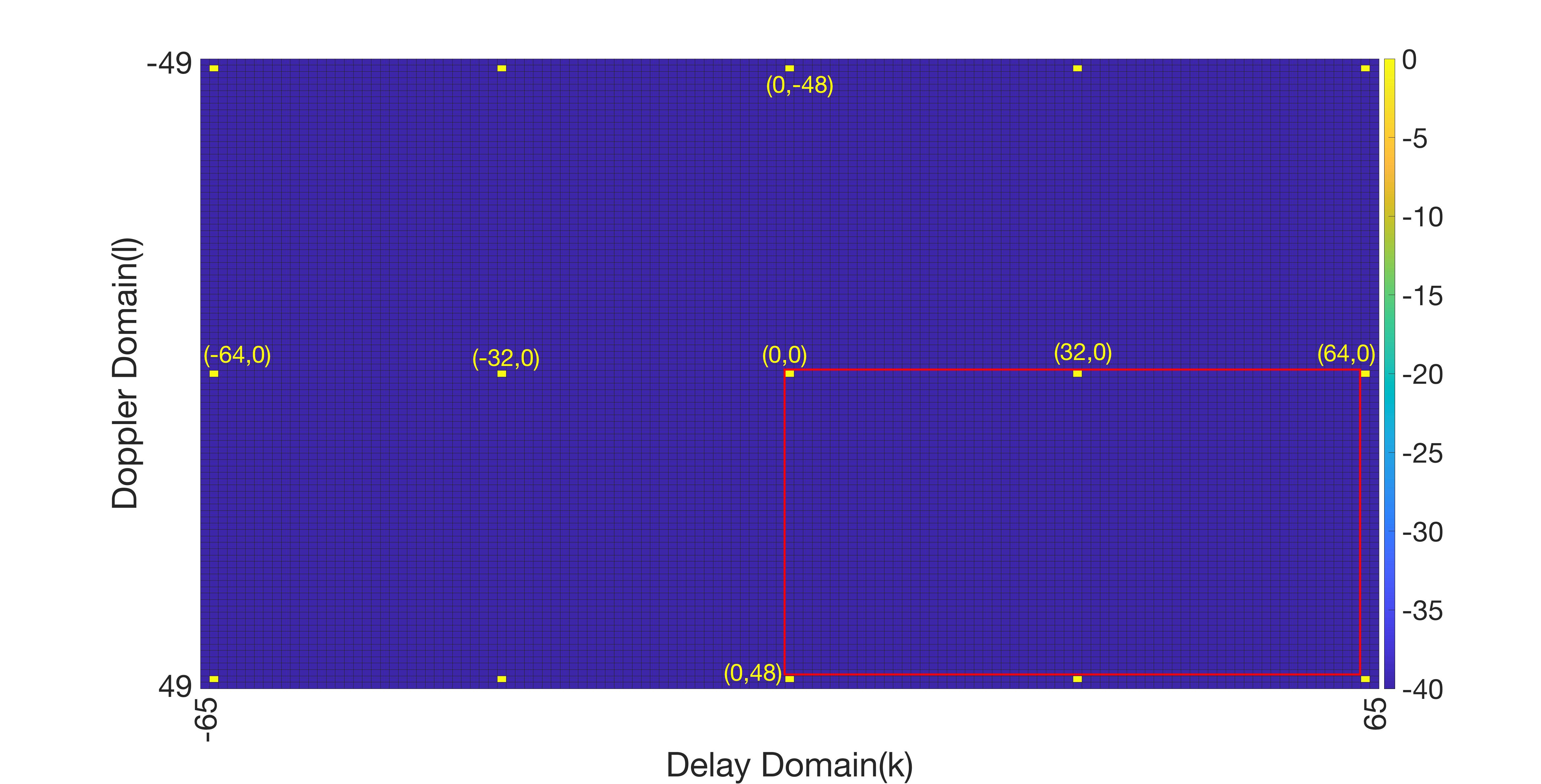
Figure 6: Heatmap showing the magnitude of the auto-ambiguity function $A_{x_{p},x_{p}}[k,l]$ of two interleaved pilots ($Q=2$) at $(0,0)$ and $(32,0)$ ($M=64$, $N=24$ ). The pilot spacing is regular ($M/2=32$), hence the auto-ambiguity function has period $2N=48$ along the Doppler axis.

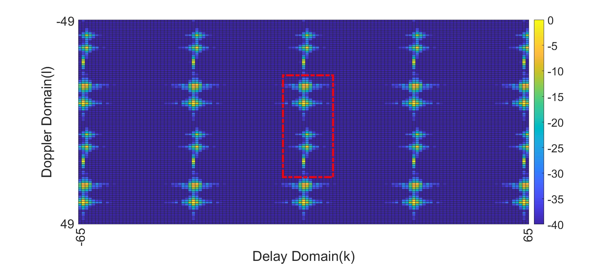
Figure 7: Heatmap showing the magnitude of the cross-ambiguity function $A_{y,x_{p}}[k,l]$ for two interleaved pilots ($Q=2$) at $(0,0)$ and $(32,0)$ ($M=64$, $N=24$ ). Six path Veh-A channel model [22] with maximum Doppler shift $\nu_{max}=6$ KHz and $\nu_{p}=7.5$ KHz. Two interleaved pilots separated by $M/2=32$ along delay axis. The Doppler spread $2\nu_{max}=12$ KHz satisfies $\nu_{p}<2\nu_{max}\leq 2\nu_{p}$. An accurate estimate for the effective channel $h_{\mbox{\scriptsize{eff}}}[k,l]$ can be read off from samples of the cross-ambiguity function within the support ${\mathcal{S}}$ of the effective channel (rectangle with red boundary).

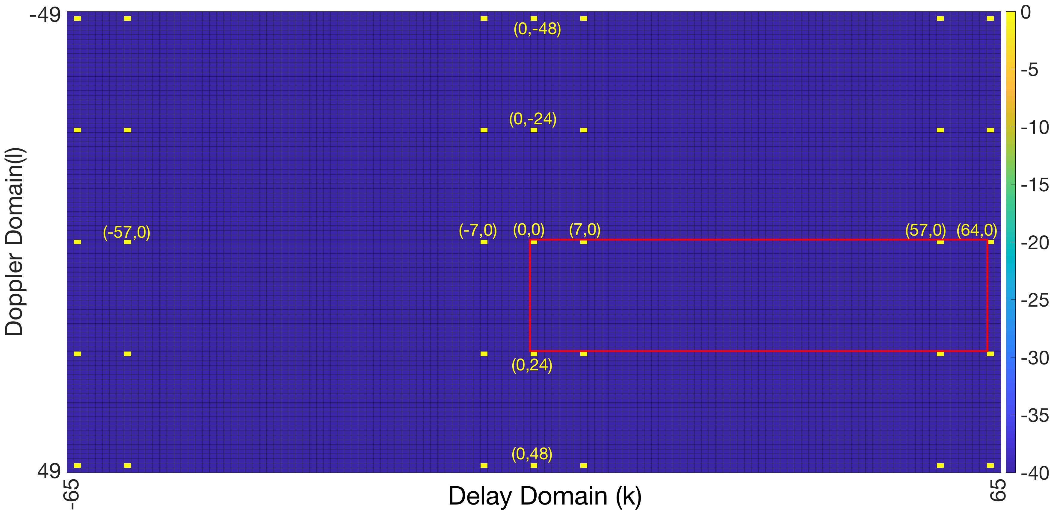
Figure 8: Heatmap showing the magnitude of the auto-ambiguity function $A_{x_{p},x_{p}}[k,l]$ when the pilot signal consists of two interleaved pilots ($Q=2$) at $(0,0)$ and $(7,0)$. $M=64$, $N=24$ and the pilot spacing along the delay axis is not equal to $M/2$. The period of the auto-ambiguity function along the Doppler axis is $N$ rather than $2N$ (see (V) for the precise non-zero locations of the auto-ambiguity function).

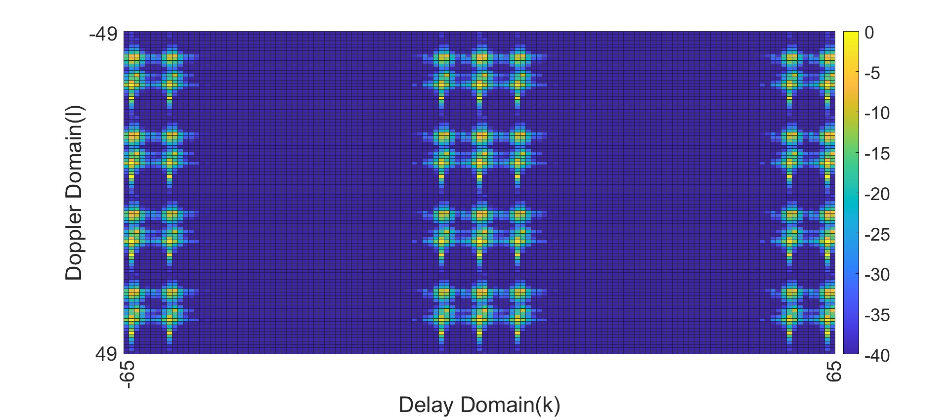
Figure 9: Heatmap showing the magnitude of the cross-ambiguity function $A_{y,x_{p}}[k,l]$ for two interleaved pilots ($Q=2$) at $(0,0)$ and $(7,0)$ with $M=64$, $N=24$. Six path Veh-A channel model [22] with maximum Doppler shift $\nu_{max}=6$ KHz and $\nu_{p}=7.5$ KHz. Note that the Doppler spread $2\nu_{max}=12$ KHz satisfies $\nu_{p}<2\nu_{max}\leq 2\nu_{p}$. The pilot spacing along the delay axis is not equal to $M/2$ and the period of the auto-ambiguity function along the Doppler axis is $N$ rather than $2N$. Aliasing of the responses $h_{0,0}^{(i)}[k,l]$ and $h_{0,1}^{(i)}[k,l]$ prevents accurate acquisition of the effective channel $h_{\mbox{\scriptsize{eff}}}[k,l]$ (compare this heatmap with the heatmap in Fig. 7 where there is no aliasing).

We see from (31) that the complexity of ML estimation using the cross-ambiguity $A_{y,x_{p}}[k,l]$ is $O(M^{2}N^{2})$. This compares unfavorably with the $O(MN)$ complexity of solving the linear system proposed in Sections III and IV. Although linear estimation is sub-optimal, numerical simulations in Section VI show that it achieves BER close to that achieved with cross-ambiguity based estimation when the effective crystallization condition is satisfied.

Finally we analyze how estimation accuracy of the proposed linear estimation in Section III and Section IV depends on the spacing between the interleaved pilots. For simplicity, we take $Q=2$ and apply linear estimation. The determinant $\Delta$ of the $2\times 2$ linear system satisfies $|\Delta|=\frac{E_{p}}{2}\left|e^{-j2\pi\frac{k_{p_{1}}}{M}}\,-\,e^{-j2\pi\frac{k_{p_{2}}}{M}}\right|$. As the minimum pilot spacing $\min\left(\left|k_{p_{1}}-k_{p_{2}}\right|\,,\,M-\left|k_{p_{1}}-k_{p_{2}}\right|\right)$ decreases, the determinant $\Delta$ approaches $0$, and the $2\times 2$ system becomes highly ill-conditioned. We expect estimation accuracy to degrade as the minimum pilot spacing decreases.

TABLE I: Power-delay profile of Veh-A channel model

Path number ($i$)	1	2	3	4	5	6
$\tau_{i}$ ($\mu$s)	0	0.31	0.71	1.09	1.73	2.51
Relative power ($p_{i}$) dB	0	-1	-9	-10	-15	-20

VI Numerical simulations

We report simulation results for the Veh-A channel model [22] which consists of six channel paths. The channel gains $h_{i}$ are modeled as independent zero-mean complex circularly symmetric Gaussian random variables, normalized so that $\sum\limits_{i=1}^{6}{\mathbb{E}}\left[|h_{i}|^{2}\right]=1$. Table I lists the power-delay profile for the six channel paths. The Doppler shift of the $i$-th path is modeled as $\nu_{i}=\nu_{max}\,\cos\left(\theta_{i}\right)$, where $\nu_{max}$ is the maximum Doppler shift of any path, and the variables $\theta_{i},i=1,2,\cdots,6$, are independent and uniformly distributed in $[-\pi\,,\,\pi)$.

We consider Zak-OTFS modulation with Doppler spread $\nu_{p}=7.5$ KHz, delay period $\tau_{p}=1/\nu_{p}=133.33\,\mu s$, $M=64$, $N=24$. The channel bandwidth $B=M\nu_{p}=0.48$ MHz and the subframe duration $T=N\tau_{p}=3.2$ ms. The information lattice/grid $\Lambda_{\mbox{\scriptsize{dd}}}=\{(k/B,l/T)$, $k,l\in{\mathbb{Z}}\,\}$.

The pulse shaping filter $w_{tx}(\tau,\nu)$ at the transmitter is a factorizable root raised cosine (RRC) filter given by

$$w_{tx}(\tau,\nu)=\sqrt{BT}\,rrc_{\beta_{\tau}}(B\tau)\,rrc_{\beta_{\nu}}(\nu T),$$ (37)

where $0\leq\beta_{\tau},\beta_{\nu}\leq 1$ and

$$rrc_{{}_{\beta}}(x) = \frac{\sin(\pi x(1-\beta))+4\beta x\cos(\pi x(1+\beta))}{\pi x\left(1-(4\beta x)^{2}\right)}.$$ (38)

We employ the matched filter $w_{rx}(\tau,\nu)=w_{tx}^{*}(-\tau,-\nu)\,e^{j2\pi\nu\tau}$ at the receiver. We choose roll-off factors $\beta_{\nu}=\beta_{\tau}=0.6$ so that the effective bandwidth of the Zak-OTFS subframe is $B^{\prime}=(1+\beta_{\tau})B$ and the effective time duration is $T^{\prime}=(1+\beta_{\nu})T$.

We employ MMSE equalization of the matrix-vector form of the Zak-OTFS I/O relation to detect information symbols at the receiver (for more details, see [1]).

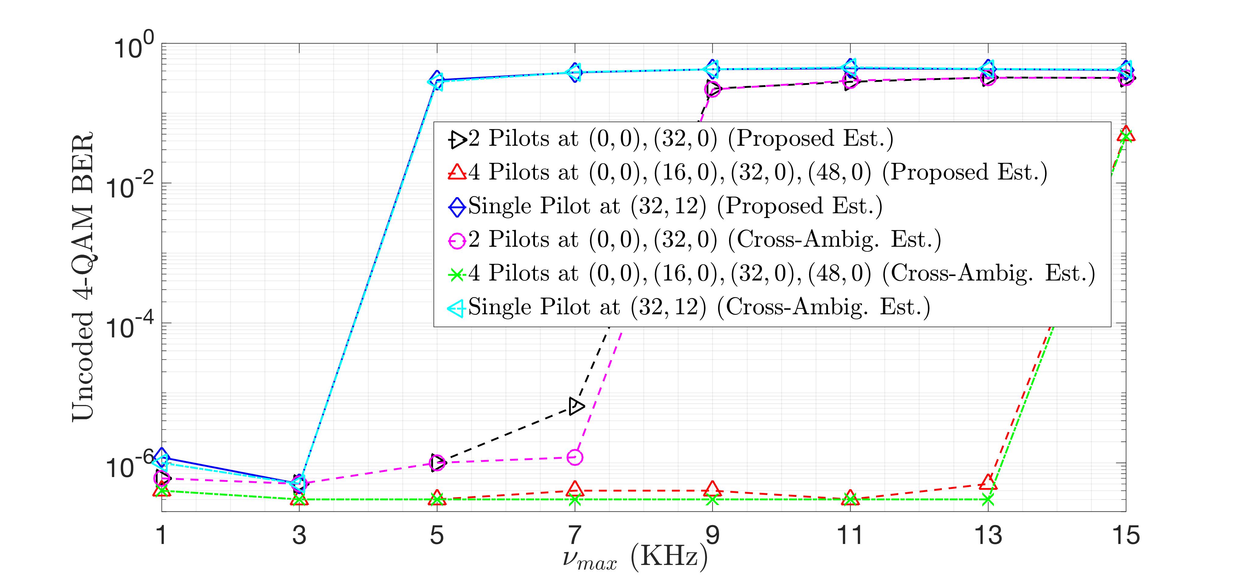
Figure 10: Uncoded $4$-QAM BER as a function of increasing $\nu_{max}$. One, two and four interleaved pilots spaced apart regularly.

Fig. 10 plots bit error rate (BER) of uncoded $4$-QAM as a function of increasing $\nu_{max}$. The ratio of pilot to data power (PDR) is $5$ dB and the ratio of received signal power to noise power (data SNR) is $25$ dB. Discrete delay spread $k_{max}=2$. We plot the BER with channel estimates acquired using the proposed linear estimation and that acquired by sampling the cross-ambiguity function $A_{y,x_{p}}[k,l]$ at DD taps in the support set of $h_{\mbox{\scriptsize{eff}}}[k,l]$.

BER performance for a single pilot (cyan and blue curves) degrade sharply for $\nu_{max}>3.5$ KHz. This is a consequence of Doppler domain aliasing as $\nu_{max}$ approaches $\nu_{p}/2=3.75$ KHz (see (II) and the discussion in Section II). By contrast, BER performance for two interleaved pilots located at $(0,0)$ and $(M/2,0)=(32,0)$ is excellent, even for a Doppler spread $2\nu_{max}=14$ KHz which is greater than $\nu_{p}=7.5$ KHz but less than $2\nu_{p}=15$ KHz. The simulation is consistent with our theoretical demonstration that two interleaved pilots can enable reliable communication when the Doppler spread $2\nu_{max}$ satisfies $\nu_{p}\leq 2\nu_{max}<2\nu_{p}$.

Fig. 10 also illustrates BER performance for $Q=4$ interleaved pilots spaced apart regularly along the delay axis (green and red curves). As expected, BER is good for Doppler spreads at most $4\nu_{p}$, i.e., $\nu_{max}<15$ KHz (see (29)). Fig. 10 also shows that the BER performance achieved with the proposed linear estimation method is almost the same as that achieved with the more complex cross-ambiguity based estimation.

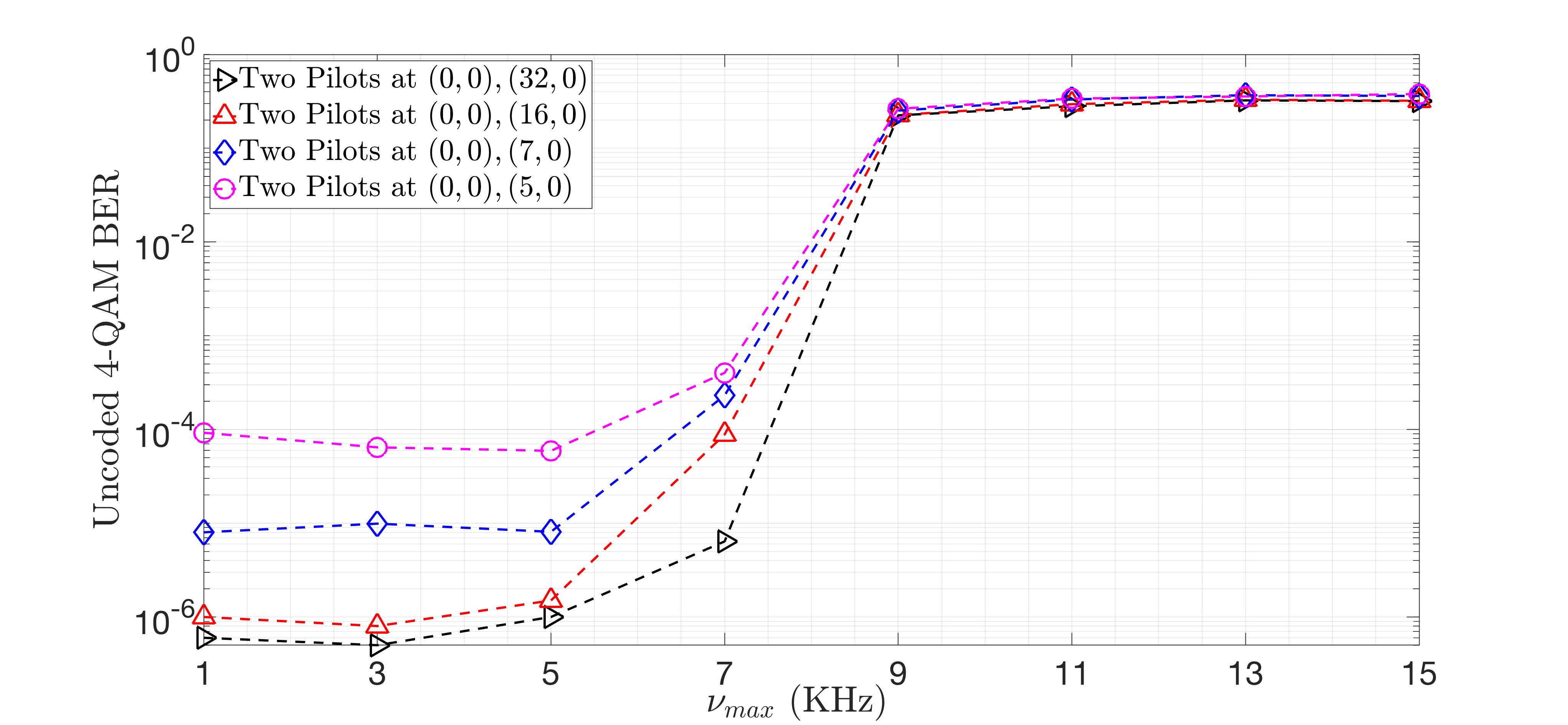
Figure 11: Uncoded $4$-QAM BER as a function of increasing $\nu_{max}$. Two interleaved pilots with irregular spacing.

Fig. 11 plots the BER performance for different spacing between two interleaved pilots. Proposed linear estimation of the taps of $h_{\mbox{\scriptsize{eff}}}[k,l]$ is considered. BER performance degrades as pilot spacing decreases, consistent with our discussion in Section V.

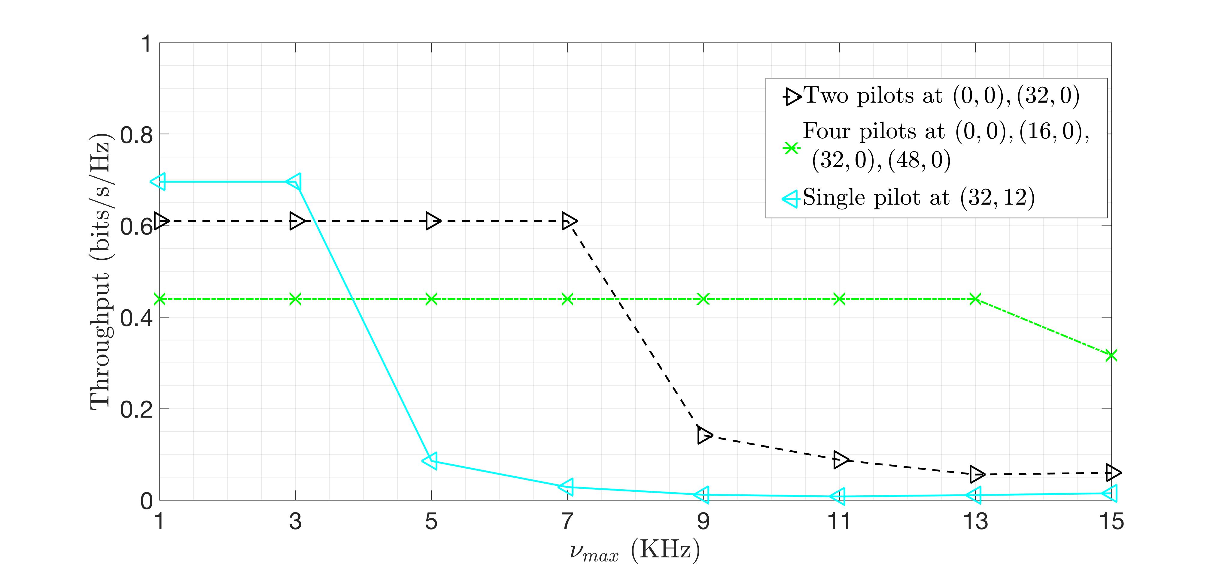
Figure 12: Effective throughput vs. $\nu_{max}$ for the same setting as in Fig. 10.

In Fig. 12 we plot the effective throughput as a function of increasing $\nu_{max}$ for the same simulation setting as in Fig. 10. Effective throughput is the ratio of the number of bits reliably communicated in each subframe to the available degrees of freedom ($B^{\prime}T^{\prime}$). The number of bits communicated reliably in a subframe is simply $(1-H(BER))$ times the number of information bits transmitted in each subframe. Here BER denotes the bit error rate and $H(\cdot)$ denotes the binary entropy function. We maximize effective throughput by interleaving the minimum number of pilots required to accurately estimate the effective channel. We minimize the number of pilots to avoid introducing unnecessary guard and pilot regions that would reduce effective throughput. When $2\nu_{max}<\nu_{p}$ we use a single pilot, when $\nu_{p}<2\nu_{max}<2\nu_{p}$ we use $2$ interleaved pilots, and when $2\nu_{p}<2\nu_{max}<4\nu_{p}$ we use $4$ interleaved pilots. Note that although a higher number of interleaved pilots results in stable throughput for a wider range of Doppler spreads (i.e., extension of the region of predictable operation), the throughput achieved is smaller due to a higher pilot and guard region overhead.

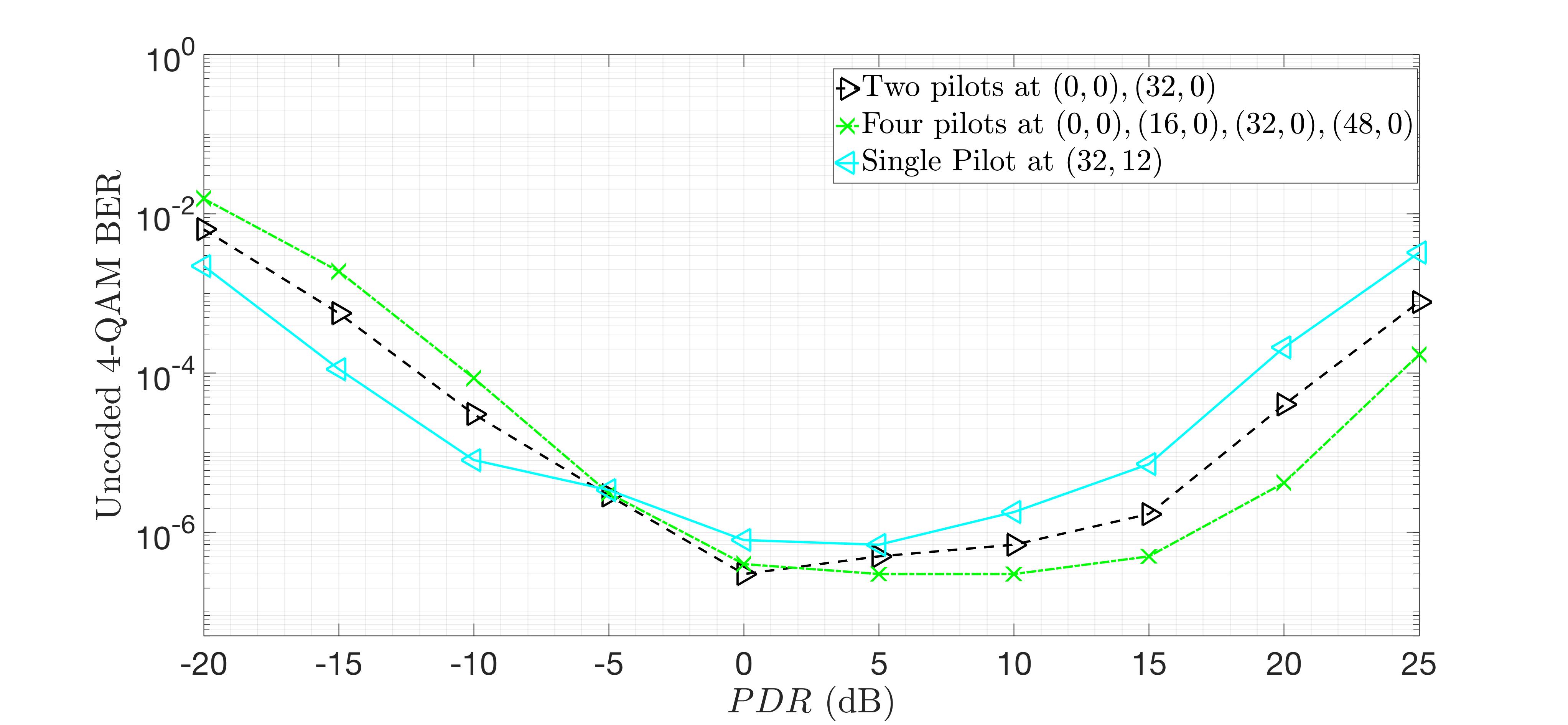
Figure 13: BER vs PDR for six-path Veh-A channel used in Fig. 10 and 12, with a fixed $\nu_{max}=2.5$ KHz.

Fig. 13 illustrates BER performance as a function of increasing PDR. The characteristic “U” shape is independent of the number of interleaved pilots. At low PDR, estimation of the effective channel is inaccurate, hence BER performance is poor. As the pilot becomes stronger, effective channel estimation becomes more accurate and BER improves. When the pilot power exceeds data power, interference to data from the pilot dominates over noise, and the BER degrades as the PDR increases.

The peak to average power ratio (PAPR) of the transmitted TD pilot (no data transmission) depends on the number of interleaved pilots. For the Zak-OTFS system considered here, the PAPR decreases from $19.4$ dB, to $16.4$ dB to $13.4$ dB as the number of interleaved pilots increases from $1$, to $2$, to $4$. This reduction is illustrated in Fig. 14. When the number of interleaved pilots doubles, the separation between pulses in the TD pilot pulse train halves. There are twice as many pulses, and each pulse is scaled down by $\sqrt{2}$ to maintain constant average power. Hence the PAPR is halved with every doubling of the number of interleaved pilots.

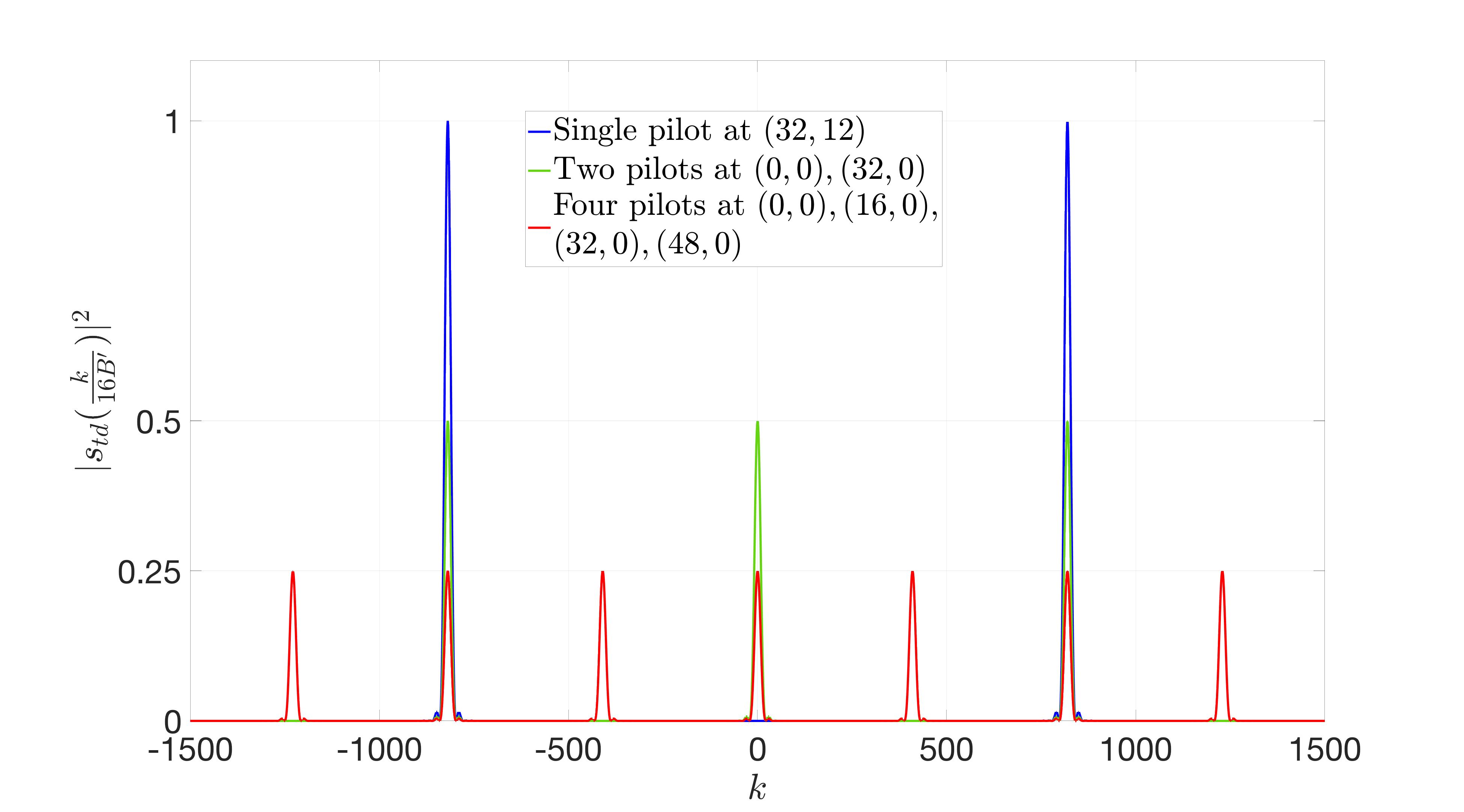
Figure 14: Energy of the TD samples of interleaved pilot samples (sampled at rate $16B^{\prime}$) for the Zak-OTFS system parameters considered in this Section VI.

VII Conclusions

We have introduced a framework for pilot design in the DD domain which makes it possible to support users with very different delay-Doppler characteristics when it is not possible to choose a single delay and Doppler period to support all users. We have translated the problem of I/O reconstruction to that of designing an interleaved pilot consisting of Zak-OTFS carriers which are selected so that in combination they produce zeros in the auto-ambiguity function of the interleaved pilot. When the interleaved pilots are spaced regularly, the auto-ambiguity function is supported on a sub-lattice of the information grid, and the I/O relation can be reconstructed from the restriction of the cross-ambiguity function (between the received and the transmitted interleaved pilot) to any fundamental region of this sub-lattice. Since the nominal complexity of computing the cross-ambiguity is high, we have introduced a method of estimating the I/O relation that only requires solving a small system of linear equations.

References

- [1] S. K. Mohammed, R. Hadani, A. Chockalingam, and R. Calderbank, “OTFS – Predictability in the delay-Doppler domain and its value to communications and radar sensing,” IEEE BITS the Information Theory Magazine, IEEE early access, doi: 10.1109/MBITS.2023.3319595, Sep. 2023.
- [2] T. Wang, J. G. Proakis, E. Masry and J. R. Zeidler, “Performance Degradation of OFDM Systems due to Doppler Spreading,” IEEE Trans. on Wireless Commun., vol. 5, no. 6, June 2006.
- [3] “Framework and Overall Objectives of the Future development of IMT for 2030 and beyond,” ITU-R M.2160-0, Nov. 2023. https://www.itu.int/rec/R-REC-M.2160/en.
- [4] H. Tataria, M. Shafi, A. F. Molisch, M. Dohler, H. Sjöland, and F. Tufvesson, “6G wireless systems: Vision, requirements, challenges, insights, and opportunities,” Proceedings of the IEEE, vol. 109, no. 7, pp. 1166-1199, Jul. 2021.
- [5]
- [6] C. -X. Wang, X. You, X. Gao, X. Zhu, Z. Li, C. Zhang, H. Wang, Y. Huang, Y. Chen, H. Haas, J. S. Thompson, E. G. Larsson, M. Di Renzo, W. Tong, P. Zhu, X. Shen, H. V. Poor, and L. Hanzo, “On the road to 6G: Visions, requirements, key technologies, and testbeds,” IEEE Commun. Surveys & Tuts., vol. 25, no. 2, pp. 905-974, 2023.
- [7] R. Hadani et al., “Orthogonal time frequency space modulation,” Proc. IEEE WCNC’2017, pp. 1-6, Mar. 2017.
- [8] A. Monk, R. Hadani, M. Tsatsanis, and S. Rakib, “OTFS - orthogonal time frequency space: a novel modulation meeting 5G high mobility and massive MIMO challenges,” arXiv:1608.02993 [cs.IT] 9 Aug. 2016.
- [9] Z. Wei, W. Yuan, S. Li, J. Yuan, G. Bharatula, R. Hadani and L. Hanzo, “Orthogonal time-frequency space modulation: a promising next-generation waveform,” IEEE Wireless Commun. Mag., vol. 28, no. 4, pp. 136-144, Aug. 2021.
- [10] P. Raviteja, K. T. .Phan, Y. Hong and E. Viterbo, “Interference Cancellation and Iterative Detection for Orthogonal Time Frequency Space Modulation,” IEEE Trans. on Wireless Comm., vol. 17, no. 10, Oct. 2018.
- [11] L. Gaudio, M. Kobayashi, G. Caire and G. Colavolpe, “On the Effectiveness of OTFS for Joint Radar Parameter Estimation and Communication,” IEEE Trans. on Wireless Comm., vol. 19, no. 9, Sept. 2020.
- [12] P. Raviteja, K. T. Phan, Y. Hong, and E. Viterbo, “Embedded pilot aided channel estimation for OTFS in delay-Doppler channels,” IEEE Trans. Veh. Tech., vol. 68, no. 5, pp. 4906-4917, May 2019.
- [13] W. Yuan et al., “Best readings in orthogonal time frequency space (OTFS) and delay Doppler signal processing,” Jun. 2022. https://www.comsoc.org/publications/best-readings/orthogonal-time-frequency-space-otfs-and-delay-doppler-signal-processing.
- [14] J. Zak, “Finite translations in solid state physics,” Phy. Rev. Lett., vol. 19, pp. 1385–1387, 1967.
- [15] A. J. E. M. Janssen, “The zak transform: A signal transform for sampled time-continuous signals,” Philips J. Res., vol. 43, pp. 23–69, 1988.
- [16] S. K. Mohammed, “Derivation of OTFS modulation from first principles,” IEEE Trans. Veh. Tech., vol. 70, no. 8, pp. 7619-7636, Aug. 2021.
- [17] S. K. Mohammed, “Time-domain to delay-Doppler domain conversion of OTFS signals in very high mobility scenarios,” IEEE Trans. Veh. Tech., vol. 70, no. 6, pp. 6178-6183, Jun. 2021.
- [18] S. K. Mohammed, R. Hadani, A. Chockalingam, and R. Calderbank, “OTFS – A mathematical foundation for communication and radar sensing in the delay-Doppler domain,” IEEE BITS the Information Theory Magazine, vol. 2, no. 2, pp. 36-55, 1 Nov. 2022.
- [19] F. Lampel, A. Avarado and F. M. J. Willems, “On OTFS using the Discrete Zak Transform,” 2022 IEEE International Conference on Communications Workshops (ICC Workshops), Seoul, Korea, Republic of, 2022.
- [20] S. Gopalam, I. B. Collings, S. V. Hanly, H. Inaltekin, S. R. B. Pillai and P. Whiting, “Zak-OTFS Implementation via Time and Frequency Windowing,” IEEE Transactions on Communications, Early Access, Feb. 2024.
- [21] M. Ubadah, S. K. Mohammed, R. Hadani, S. Kons, A. Chockalingam, and R. Calderbank, “Zak-OTFS for integration of sensing and communication,” available online: arXiv:2404.04182v1 [eess.SP] 5 Apr 2024.
- [22] ITU-R M.1225, “Guidelines for evaluation of radio transmission technologies for IMT-2000,” International Telecommunication Union Radio communication, 1997.
- [23] S. Gopalam, H. Inaltekin, I. B. Collings and S. V. Hanly, “Optimal Zak-OTFS Receiver and Its Relation to the Radar Matched Filter,” IEEE Open Journal of the Communications Society, Early Access, June 2024.