Improvement of Bayesian PINN Training Convergence in Solving Multi-scale PDEs with Noise

Abstract

Bayesian Physics Informed Neural Networks (BPINN) have received considerable attention for inferring differential equations’ system states and physical parameters according to noisy observations. However, in practice, Hamiltonian Monte Carlo (HMC) used to estimate the internal parameters of BPINN often encounters troubles, including poor performance and awful convergence for a given step size used to adjust the momentum of those parameters. To improve the efficacy of HMC convergence for the BPINN method and extend its application scope to multi-scale partial differential equations (PDE), we developed a robust multi-scale Bayesian PINN (dubbed MBPINN) method by integrating multi-scale deep neural networks (MscaleDNN) and Bayesian inference. In this newly proposed MBPINN method, we reframe HMC with Stochastic Gradient Descent (SGD) to ensure the most “likely” estimation is always provided, and we configure its solver as a Fourier feature mapping-induced MscaleDNN. The MBPINN method offers several key advantages: (1) it is more robust than HMC, (2) it incurs less computational cost than HMC, and (3) it is more flexible for complex problems. We demonstrate the applicability and performance of the proposed method through general Poisson and multi-scale elliptic problems in one- to three-dimensional spaces. Our findings indicate that the proposed method can avoid HMC failures and provide valid results. Additionally, our method can handle complex PDE and produce comparable results for general PDE. These findings suggest that our proposed approach has excellent potential for physics-informed machine learning for parameter estimation and solution recovery in the case of ill-posed problems.

Introduction

Partial differential equations (PDE) have extensive applications across various fields, as they model complex systems’ physical properties and behaviors. The parameters within these PDEs often represent key physical properties of the system under study (?). The inverse problem involves estimating these parameters or recovering the solution based on observations and limited constraints, which can provide insights into the underlying physical phenomena (?). In the context of well-posed problems, physics-informed neural networks (PINN) have demonstrated significant success in accurately estimating these parameters. However, in ill-posed problems, where the observations may be noisy or incomplete, traditional numerical solvers often fail to provide reliable solutions (?). To address these challenges, statistical and machine learning tools, such as regularizers, handle the ill-posed inverse problems by selecting or weighting variables (?; ?). As a natural regularization approach, Bayesian statistics has numerous applications in dealing with noisy and high-dimensional data (?). By integrating Bayesian statistics with PINN, some researchers have proposed robust methodologies for estimating parameters from real-world observational data in linear or nonlinear systems, thereby enhancing the accuracy and reliability of the analysis (?; ?; ?).

BPINN

In terms of the solution for the inverse problem governed by PDE, to improve the capacity of PINN for separating the system states and the noise from real-world noisy observations, we need to estimate reasonably the internal parameters of PINN and system parameters based on those observations. Bayesian statistics offers effective inference methods for noisy and incomplete data (?). By treating the parameters of interest as random variables instead of deterministic values, Bayesian statistics ultimately provides a distribution conditioned on observations as the inference of these parameters. When seeking a point estimate, such as the estimation of PINN parameters, Bayesian statistics regularizes the parameters so that functional parameters receive more weight, thereby controlling the error (?).

Consequently, Bayesian PINN is proposed using Bayesian statistics to estimate PINN parameters. Considering noise sampled from mean zero, i.i.d. normal distributions, BPINN uses Bayesian statistics as the estimation method and treats the likelihood accordingly. Finally, it employs Hamiltonian Monte Carlo (HMC) or variational inference (VI) for posterior sampling. This framework successfully quantifies uncertainty and improves predictions in noisy environments.

HMC, VI

Assuming the prior of BPINN as a Gaussian Process with mean 0 as the amount of parameters goes to infinity, we know that the posterior should also follow a multivariate Gaussian distribution (?; ?). Since the posterior distribution has no analytical solution, it could only be approximated. Generally, two ways of approximating the posterior distribution are the HMC and VI methods.

The HMC method enhances the Markov Chain Monte Carlo (MCMC) method. The new step of HMC is generated by solving the Hamiltonian system instead of a random walk in MCMC, but the acceptance procedure of each new step remains the same (?; ?; ?). HMC is more efficient than MCMC by higher acceptance rate, but the computational cost remains high (?).

VI assumes that the posterior distribution belongs to a family of parameterized distributions. In other words, VI uses functions with a different parameterization to approximate the posterior distribution. By updating the parameters from this different parameterization, VI minimizes the KL divergence between the posterior distribution and its approximation. VI considers the optimal solution of this deterministic optimization problem as the best approximation of the posterior distribution (?; ?)

This paper chooses HMC over VI for theoretical and practical reasons. Theoretically, VI is projecting the posterior distribution onto a new function class, which is usually assumed to be the mean-field Gaussian approximation by the deep learning community (?; ?). Therefore, VI does not offer the same theoretical guarantees as MCMC approaches. Practically, lots of papers show that HMC has better performance than VI. For example, in high-dimensional problems (?) showing HMC’s superiority over VI and challenges.

Objective

Since the establishment of BPINN, they have demonstrated remarkable performance in solving mathematical problems in scientific computations and engineering applications based on their great potential in integrating prior knowledge with data-driven approaches. For example, utilizing BPINN to quantify uncertainties in the predictions of physical systems modeled by differential equations (?; ?), inverse problems (?; ?; ?), nonlinear dynamical system (?), etc.

After that, significant efforts have been undertaken to improve BPINN’s performance in two main areas: the improvement of posterior sampling methods and the choice of NN-solver. In terms of the sampling strategy, one approach is to reduce the computational cost of the MCMC method (?; ?), and the other approach is to breach the gap between MCMC and VI through a particle-based VI approach. In the context of BPINN, methods like Stein Variational Gradient Descent (SVGD) (?) and Ensemble Kalman inversion (EKI) (?; ?; ?) has been proposed for sparse and noisy data. In terms of the latter one, the authors in (?) reconstructed the solver of PINN by extending the output pipelines and ensembled the multiple outputs at the same point to calculate statistical properties, then imposed any prior knowledge or assumptions regarding the uncertainty of the data. A Generative Adversarial Networks model is configured as the BPINN (BPI-GAN) solver to learn flexible low-dimensional functional priors, e.g., Gaussian and non-Gaussian processes. BPI-GAN is easy to apply to big data problems by enabling mini-batch training using stochastic HMC or normalizing flows (?). To robustly address multi-objective and multi-scale problems, a novel methodology for automatic adaptive weighting of Bayesian Physics-Informed Neural Networks, which automatically tunes the weights by considering the multitask nature of target posterior distribution (?).

In practice, we found that HMC is sensitive to the step size of updating parameters and sometimes does not converge to a stable distribution. The step size used when updating the parameter serves as momentum size in the Hamiltonian system. When this step size is too large, the sum of the log-likelihood of the parameters goes to infinity, and the algorithm breaks down. However, there are no explicit standards for measuring step size. That is to say, one specific step size may work for a PDE but fail for a different PDE. Even for the same PDE, changing the step size could significantly impact the performance of BPINN.

Additionally, as in the aforementioned BPINN, the solvers are configured as a vanilla deep neural networks (DNN) model, then their performance will be limited by the spectral bias or frequency preference of DNN, and they may encounter some dilemmas for addressing complex problems, such as recovering the solution of multi-scale PDEs from noisy data. Recently, a multi-scale DNN (MscaleDNN) was developed to address the limitation of traditional DNNs, which can easily capture the low-frequency components of target functions but struggle to accurately represent high-frequency components (?; ?). Furthermore, utilizing a Fourier feature embedding consisting of sine and cosine can improve the capacity of DNN; These enhanced DNNs help mitigate the issue of spectral bias, enabling the networks to more effectively learn and represent high-frequency components (?; ?; ?; ?).

In this paper, we propose a novel estimation method to address the convergence problems of classical HMC by integrating Stochastic Gradient Descent (SGD) into the original HMC framework. Compared to the classical BPINN-HMC, this new approach ensures point estimation of the parameters with significantly lower computational costs. We apply this method across various PDE problems, including linear and nonlinear Poisson equations and general and multi-scale PDE. Additionally, we introduce the MBPINN approach by incorporating a Fourier feature mapping (FFM) to enhance the overall workflow further. The integrated MBPINN_SGD method demonstrates strong potential and robustness in these complex scenarios.

Formulation and Failure of Classical BPINN

Formulation of BPINN

This subsection briefly introduces the formulation of BPINNs first proposed in (?). Given a $d$-dimensional domain $\Omega$ and its boundary $\partial\Omega$, let us consider the following system of parametrized PDEs:

$$\mathcal{N}_{\bm{\lambda}}[u(\bm{x})]=f(\bm{x}),~{}\quad\bm{x}\in\Omega$$ (1)

$$\mathcal{B}[u\left(\bm{x}\right)]=g(\bm{x}),\quad\quad\bm{x}\in\partial\Omega$$

in which $\mathcal{N}_{\bm{\lambda}}$ stands for the linear or nonlinear differential operator with parameters $\bm{\lambda}$, $\mathcal{B}$ is the boundary operators. Generally, the sampling data of force term $f(\bm{x})$ and boundary function $g(\bm{x})$ may be disturbed by unanticipated noise for real applications. The available dataset $\mathcal{D}$ composed by the collocation points and the corresponding evaluation of $f$ and $g$ for this scenario is given by

$$\mathcal{D}=\mathcal{D}_{f}\cup\mathcal{D}_{g}$$ (2)

with $\mathcal{D}_{f}=\{(\bm{x}_{f}^{(i)},\tilde{f}^{(i)})\}_{i=1}^{N_{f}}$ and $\mathcal{D}_{g}=\{(\bm{x}_{g}^{(i)},\tilde{g}^{(i)})\}_{i=1}^{N_{g}}$. The measurements are i.i.d Gaussian random variables, i.e.,

$$\tilde{f}^{(i)} =f(\bm{x}_{f}^{(i)})+\varepsilon_{f}^{(i)},\quad i=1,2,\ldots,N_{f},$$ (3)

$$\tilde{g}^{(i)} =g(\bm{x}_{g}^{(i)})+\varepsilon_{g}^{(i)},\quad i=1,2,\ldots,N_{g},$$

where $\varepsilon_{f}^{(i)}$ and $\varepsilon_{g}^{(i)}$ are independent mean-zero Gaussian noise with given standard deviations $\sigma_{f}$ and $\sigma_{g}$, respectively. Note that the noise size could differ among measurements of different terms and even between measurements of the same terms in the PDE.

The Bayesian framework starts from representing $u$ with a surrogate model $\tilde{u}(\bm{x};\bm{\theta})$, where $\bm{\theta}$ is the vector of parameters in the surrogate model with a prior distribution $P(\bm{\theta})$. When the process of the Bayesian method meets the physics-informed neural networks, the architecture of BPINN is constructed, and its surrogate model is configured as a general DNN. Mathematically, the classical DNN defines the following mapping

$$\mathcal{F}:\bm{x}\in\mathbb{R}^{d}\Longrightarrow\bm{y}=\mathcal{F}(x)\in\mathbb{R}^{c}$$ (4)

with $d$ and $c$ being input and output dimensions, respectively. The DNN function $\mathcal{F}$ is a nested composition of sequential single linear functions and nonlinear activation functions, which is in the form of

$$\begin{cases}\bm{y}^{[0]}=\bm{x}\\ \bm{y}^{[\ell]}=\sigma\circ(\bm{W}^{[\ell]}\bm{y}^{[\ell-1]}+\bm{b}^{[\ell]}),~{}~{}\text{for}~{}~{}\ell=1,2,3,\cdots\cdots,L\end{cases}$$

where $\bm{W}^{[\ell]}\in\mathbb{R}^{n_{\ell+1}\times n_{\ell}},\bm{b}^{[\ell]}\in\mathbb{R}^{n_{\ell+1}}$ are the weights and biases of $\ell$-th hidden layer, respectively, $n_{0}=d$ and $n_{L+1}$ is the dimension of output, and $``\circ"$ stands for the elementary-wise operation. The function $\sigma(\cdot)$ is an element-wise activation function. We denote the output of a DNN by $\bm{y}(\bm{x};\bm{\theta})$ with $\bm{\theta}$ representing the parameter set of $\bm{W}^{[1]},\cdots\bm{W}^{[L]},\bm{b}^{[1]},\cdots\bm{b}^{[L]}$.

Consequently, with the physical constraints, Bayes’ theorem under the context of BPINNs can be formulated as follows:

$$P(\theta|\mathcal{D})=\frac{P(\mathcal{D}|\theta)P(\theta)}{P(\mathcal{D})}\simeq P(\mathcal{D}|\theta)P(\theta).$$ (5)

Then, the log-likelihood can be calculated as:

$$\log P(\mathcal{D}|\bm{\theta})=\log P(\mathcal{D}_{f}|\bm{\theta})+\log P(\mathcal{D}_{b}|\bm{\theta}),$$ (6)

with

$$P(\mathcal{D}_{f}|\bm{\theta})=\prod_{i=1}^{N_{f}}\frac{1}{\sqrt{2\pi\sigma_{f}^{(i)}{}^{2}}}\exp\left(-\frac{\left(\mathcal{N}_{\bm{\lambda}}[\tilde{u}(\bm{x}_{f}^{(i)};\theta)]-\tilde{f}^{(i)}\right)^{2}}{2\sigma_{f}^{(i)}{}^{2}}\right)$$ (7)

and

$$P(\mathcal{D}_{g}|\bm{\theta})=\prod_{i=1}^{N_{b}}\frac{1}{\sqrt{2\pi\sigma_{g}^{(i)}{}^{2}}}\exp\left(-\frac{\left(\mathcal{B}[u\left(\bm{x}_{g}^{(i)};\bm{\theta}\right)]-\tilde{g}^{(i)}\right)^{2}}{2\sigma_{g}^{(i)}{}^{2}}\right).$$ (8)

Finally, we decide whether to accept this step based on the calculation of (6) and the log-likelihood of the prior.

Failure of BPINN

HMC-driven BPINN method (BPINNHMC) has shown its remarkable performance in solving PDEs, as demonstrated in (?). However, the HMC algorithm’s convergence appears problematic when we extend BPINN to solve more complex PDE problems. The main issues are that the performance of BPINN is poor, and sometimes HMC does not converge, providing us with no results.

To illustrate these two problems, we introduce a concrete example in the context of multi-scale elliptic PDEs. Consider the 1-dimensional elliptic equation with homogeneous Dirichlet boundary conditions in $\Omega=[0,1]$:

$$\begin{cases}-\frac{d}{dx}\left(A^{\varepsilon}(x)\frac{d}{dx}u^{\varepsilon}(x)\right)=f(x),\\ u^{\varepsilon}(0)=u^{\varepsilon}(1)=0,\end{cases}$$ (9)

in which

$$A^{\varepsilon}(x)=\frac{1}{2+\cos\left(2\pi x/\varepsilon\right)},$$ (10)

with $\varepsilon>0$ being a small constant and $f(x)=1$. Under these conditions, a unique solution is given by

$$\begin{split}u^{\varepsilon}(x)&=x-x^{2}+\varepsilon\left(\frac{1}{4\pi}\sin\left(2\pi\frac{x}{\varepsilon}\right)-\frac{1}{2\pi}x\sin\left(2\pi\frac{x}{\varepsilon}\right)-\right.\\ &\left.\frac{\varepsilon}{4\pi^{2}}\cos\left(2\pi\frac{x}{\varepsilon}\right)+\frac{\varepsilon}{4\pi^{2}}\right).\end{split}$$

We employ the classical BPINN_HMC method to solve the above problem with $\varepsilon=0.5$ and $\varepsilon=0.1$. For this study, we utilize 50 observations for system state and force term in $\Omega$ to recover the solution of (9). Meantime, 1000 equidistant points are sampled in $\Omega$ to evaluate this method. The DNN solver comprises two hidden layers, each containing 30 hidden units. The activation function used in all hidden layers is the sine function, while the output layers are linear. To estimate the internal parameters of the BPINN, we run the BPINN_HMC method for 600 epochs and obtain the posterior distribution by the results of the latter 500 epochs. Figure 1 demonstrates the performance of the BPINN-HMC method for both smooth case ($\varepsilon=0.5$) and slight oscillation case($\varepsilon=0.1$) when the noise level is 0.01. This classical method will fail to capture the exact solution for the oscillation case.

Table 1: The influence of step size for classic BPINN-HMC when $\varepsilon=0.5$ and noise level is 0.01, 0.05 and 0.1, respectively.

$\varepsilon$	Noise	step size	0.001	0.0005	0.0001	0.00005	0.00001
0.5	0.01	Success/Failure	Failure	Failure	Failure	Success	Success
		REL of solution	—	—	—	0.0124	0.2161
	0.05	Success/Failure	Failure	Failure	Success	Success	Success
		REL of solution	—	—	0.0751	0.399	0.405
	0.1	Success/Failure	Failure	Success	Success	Success	Success
		REL of solution	—	0.400	0.396	0.454	0.502
0.1	0.01	Success/Failure	Failure	Failure	Failure	Success	Success
		REL of solution	—	—	—	0.412	0.390
	0.05	Success/Failure	Failure	Failure	Success	Success	Success
		REL of solution	—	—	0.394	0.399	0.405
	0.1	Success/Failure	Failure	Success	Success	Success	Success
		REL of solution	—	0.400	0.396	0.454	0.502

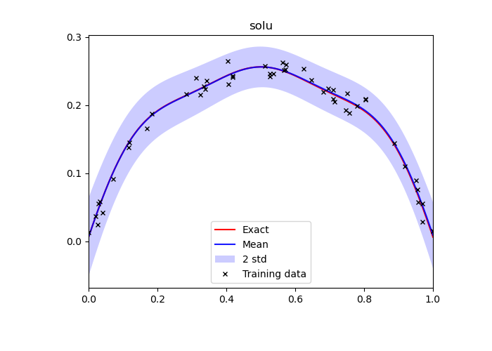
(a) $u^{\varepsilon}$ for $\varepsilon=0.5$

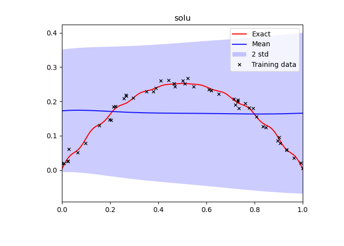
(b) $u^{\varepsilon}$ for $\varepsilon=0.1$

Figure 1: The predictions and exact solution for $\varepsilon=0.5$ and $\varepsilon=0.1$ when noise level is 0.01.

Furthermore, we perform the BPINN_HMC method with various step sizes (0.05, 0.001, 0.0005, 0.0001, 0.00001) to evaluate its robustness when the noise level is 0.01, 0.05, and 0.1, respectively. As shown in Table 1, the results indicate that the BPINN_HMC method will fail to converge and encounter errors when the step size is large for different noise levels. This further underscores the limitations of the classical BPINN_HMC method in dealing with both smooth and oscillation scenarios.

In addition, we implemented BPINN with various hyperparameter configurations, including different numbers of sampled points, burn-in points, and network sizes. However, these adjustments still did not yield satisfactory results. This observation highlights the need for additional techniques to enhance the accuracy and robustness of the BPINN method.

Methodology

SGD Reframed HMC method

In this section, to avoid the convergence failure of classic HMC, we would like to use SGD to reframe the existing method. Unlike HMC, where the entire posterior distribution of the parameters is modeled, we aim to find the set of parameters that are most “likely”, as this procedure guarantees a solution. Notice that, in each step of HMC, a likelihood is calculated for a set of parameters and is used to determine whether to accept this step. Finally, all accepted steps form the empirical posterior distribution.

Through the HMC algorithm, we could see that each set of parameters corresponds to a likelihood based on the kernel function of BPINN. We define the most “likely” set of parameters as the set that maximized the kernel function. Thus, by finding the most “likely” set of parameters, we mean seeking to find the maximum of the true distribution by viewing the inverse of the likelihood as the loss. The larger the likelihood, the smaller the loss. This method turns the problem into an optimization problem, and we use typical stochastic gradient descent (SGD), like the Adam optimization method, to find the optimum.

Algorithm 1 Adam optimization method

0:  Stepsize $\alpha$ and Exponential decay rates for the moment estimates $\beta_{1},\beta_{2}\in(0,1]$

0:  Stochastic objective function $f(\bm{\theta})$ with parameters $\bm{\theta}$

0:  Initialize the parameter vector $\bm{\theta}_{0}\neq\bm{0}$, the $1^{st}$ moment vector $\bm{m}_{0}=\bm{0}$, the $2^{nd}$ moment vector $\bm{v}_{0}=\bm{0}$ and timestep $t=0$

1:  while $\theta_{t}$ not converged do

2:     t = t+1

3:     $\bm{g}_{t}=\nabla_{\bm{\theta}}f_{t}(\bm{\theta}_{t-1})$

4:     $\bm{m}_{t}=\beta_{1}\cdot\bm{m}_{t-1}+(1-\beta_{1})\cdot\bm{g}_{t}$

5:     $\bm{v}_{t}=\beta_{2}\cdot\bm{v}_{t-1}+(1-\beta_{2})\cdot\bm{g}_{t}\odot\bm{g}_{t}$

6:     $\widehat{\bm{m}}_{t}=\bm{m}_{t}/(1-\beta_{1}^{t})$

7:     $\widehat{\bm{v}}_{t}=\bm{v}_{t}/(1-\beta_{2}^{t})$

8:     $\bm{\theta}_{t}=\bm{\theta}_{t-1}-\alpha\cdot\widehat{\bm{m}}_{t}/(\sqrt{\widehat{\bm{v}}_{t}}+\varepsilon)$

9:  end while

10:  return  $\bm{\theta}_{t}$

MBPINN

In this section, we proposed the unified architecture of MBPINN to estimate the parameters and recover the solution of PDEs according to the given observation data with unexpected noise by embracing the vanilla BPINN method with Fourier-induced multi-scale DNN.

The BPINN method’s solver is configured as a general DNN. A general DNN model can provide satisfactory solutions for low-complexity problems but faces significant challenges when addressing complex problems, such as multi-scale PDEs. Recently, a MscaleDNN model has been proposed based on the intrinsic property of DNN, that is, spectral bias or frequency preference, to mitigate the pathology of DNN by converting original data to a low-frequency space (?; ?; ?; ?). Hence, we can improve the capacity of BPINN by embracing the multi-scale DNN with Bayesian inference. A schematic diagram of MscaleDNN with multiple Fourier feature mapping (FFM) pipelines is described as follows:

$$\hat{\bm{x}} =\bm{\Lambda}_{n}\bm{x},\quad n=1,2,\ldots,N,$$ (11)

$$\bm{\zeta}_{n}(\bm{x}) =\left[\cos\left(\hat{\bm{x}}\right),\sin\left(\hat{\bm{x}}\right)\right]^{\mathrm{T}},\quad n=1,2,\ldots,N,$$

$$\bm{F}_{n}(\bm{x}) =\mathcal{FCN}\left(\bm{\zeta}_{n}(\bm{x})\right),\quad n=1,2,\ldots,N,$$

$$\bm{NN}(\bm{x}) =\bm{W}_{O}\cdot\left[\bm{F}_{1},\bm{F}_{2},\cdots,\bm{F}_{N}\right]+\bm{b}_{O},$$

where $\Lambda_{n}$ is a transmitted matrix that is consistent with the dimension of input data and the number of neural units for the first hidden layer in DNNs, and its elements are sampled from an isotropic Gaussian distribution $\mathcal{N}(0,\xi)$ with $\xi>0$ is a user-specified hyper-parameter. $\mathcal{FCN}$ stands for a fully connected neural network. $\bm{W}_{O}$ and $\bm{b}_{O}$ represent the weights and bias for the output layer of MscaleDNN, respectively.

For given multi-scale PDEs, the solution generally has the following coarse/fine decomposition, $u=u_{c}+u_{f}$, in which $u_{c}$ contains the smooth part and $u_{f}$ contains the fine details of the multi-scale solution $u$, respectively. Please refer to Figure 2.

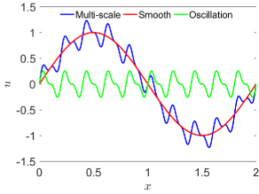
Figure 2: The decomposition of multi-scale function.

Naturally, the force term $f$ and the boundary constraint $g$ may also oscillate and decompose as $f=f_{c}+f_{f}$ and $g=g_{c}+g_{f}$. When the observations are i.i.d Gaussian random variables, i.e.,

$$\tilde{f}^{(i)} =f_{c}(x_{f}^{(i)})+f_{f}(x_{f}^{(i)})+\varepsilon_{f}^{(i)},\quad x_{f}^{(i)}\in\mathcal{D}_{f}$$

$$\tilde{g}^{(i)} =g_{c}(x_{g}^{(i)})+g_{f}(x_{g}^{(i)})+\varepsilon_{g}^{(i)},\quad x_{g}^{(i)}\in\mathcal{D}_{g},$$

where $\mathcal{D}_{f}=\{(x_{f}^{(i)},\tilde{f}^{(i)})\}_{i=1}^{N_{f}}$ and $\mathcal{D}_{g}=\{(\bm{x}_{g}^{(i)},\tilde{g}^{(i)})\}_{i=1}^{N_{g}}$. As well as, the $\varepsilon_{u}^{(i)}$, $\varepsilon_{f}^{(i)}$ and $\varepsilon_{b}^{(i)}$ are same as the aforementioned setups in section Formulation of BPINN.

Within the framework of MBPINN, the log-likelihood can be calculated as follows:

$$\log P(\mathcal{D}|\bm{\theta})=\log P(\mathcal{D}_{f}|\bm{\theta})+\log P(\mathcal{D}_{g}|\bm{\theta}),$$ (12)

with $P(\mathcal{D}_{f}|\theta)$ and $P(\mathcal{D}_{g}|\bm{\theta})$ being the same as the (7) and (8), respectively.

If some additional observed data are available inside the interested domain, $\tilde{u}^{(i)}=u_{c}(x_{u}^{(i)})+u_{f}(x_{u}^{(i)})+\varepsilon_{u}^{(i)},\quad i=1,2,\ldots,N_{u}$ and $\mathcal{D}_{u}=\{(x_{u}^{(i)},\tilde{u}^{(i)})\}_{i=1}^{N_{u}}$, then a log-likelihood term indicating the mismatch between the predictions produced by MBPINN and the observations can be taken into account:

$$P(\mathcal{D}_{u}|\theta)=\prod_{i=1}^{N_{u}}\frac{1}{\sqrt{2\pi\sigma_{u}^{(i)}{}^{2}}}\exp\left(-\frac{\left(\tilde{u}(x_{u}^{(i)};\theta)-\tilde{u}^{(i)}\right)^{2}}{2\sigma_{u}^{(i)}{}^{2}}\right).$$

Experiment

Our experiments aim to show that our MBPINN with SGD reframed HMC is indeed capable of approximating the analytical solution for given general and complex PDE based on observations with noise. The sine function is the activation function for all hidden layers, and the output layer is linear for all five methods. In addition, the BPINN method, with a DNN model as its solver, is introduced to serve as the baseline. Five types of compared methods are as follows:

• BPINN_HMC: Its solver is a normal DNN model with classical HMC posterior sampling method (?).

• FF_MBPINN_HMC: Its solver is a MscaleDNN model with an FFM pipeline with a classical HMC posterior sampling method.

• FF_MBPINN_SGD: All the same as FF_MBPINN_HMC but using SGD reframe HMC instead of HMC method.

• 2FF_MBPINN_HMC: Its solver is an MscaleDNN model with two FFM pipelines with a classical HMC posterior sampling method.

• 2FF_MBPINN_SGD: All the same as 2FF_MBPINN_HMC but using SGD reframe HMC instead of HMC method.

We keep the step size of HMC used in the above methods steady and run it for 600 epochs, then record the last 500 epochs and obtain the posterior distribution. In addition, we perform the SGD (Adam) used in the above methods with a fixed learning rate for 20000 epochs and obtain the most “likely” parameters of the FF_MBPINN_SGD and 2FF_MBPINN_SGD methods.

As for the observations, we generate them based on an equidistant sampling strategy or random sampling strategy (For example, Latin Hypercube Sampling (LHS)) in the interest domain. We also add noise based on different noise levels. Noise level is defined by the constant times of a standard normal distribution. For example, the noise level 0.1 means $0.1*\mathcal{N}(0,1)$.

To quantitatively measure the performance of our model, we compute the Relative Error (REL) between the mean-predicted and the exact solutions. The REL is calculated as follows:

$$\text{REL}=\sqrt{\frac{\sum_{i=1}^{N^{\prime}}|\hat{u}(x_{i}^{\prime})-u^{*}(x_{i}^{\prime})|^{2}}{\sum_{i=1}^{N^{\prime}}|u^{*}(x_{i}^{\prime})|^{2}}},$$

where $\hat{u}(x_{i}^{\prime})$ denotes the mean-predicted solution at point $x_{i}^{\prime}$, $u^{*}(x_{i}^{\prime})$ is the exact solution, and $N^{\prime}$ is the total number of evaluation points.

Example 1.

We now consider the following nonlinear Poisson problem with two frequency components in $\Omega=[0,1]$:

$$\begin{cases}0.01\Delta u(x)+k(x)u(x)=f(x)\\ u(0)=u(1)=0.1\end{cases}$$

with a coefficient term $k(x)$ as follows

$$k(x)=0.1+\exp\left(-0.5\frac{(x-0.5)^{2}}{0.15^{2}}\right).$$

An exact solution is given by

$$u_{\text{true}}(x)=\sin(2\pi x)+0.1\cos(10\pi x),$$

and it naturally induces the force term

$$f(x)=0.01\left(-4\pi^{2}\sin(2\pi x)-10\pi^{2}\cos(10\pi x)\right)+k(x)\cdot u(x).$$

We solve the above two-scale problem by employing the five methods above, with its solvers having two hidden layers, and each layer has 30 units. In this example, the 50 observations located randomly in $\Omega$ for the solution and force side are disturbed with mean-zero Gaussian distributed noise. In addition, the 25 observations located randomly in $\Omega$ for the coefficient term, $k(x)$, are also disturbed. To recover the solution and coefficient term simultaneously, two ansatzes expressed by DNN are used in BPINN_HMC, and two ansatzes expressed by MscaleDNN with FFM pipelines are used in other methods. The $\Lambda$ of FF_MBPINN is set as 10 and 2 for solution and coefficient, respectively. The $\Lambda_{1}$ and $\Lambda_{2}$ of FF_MBPINN for solution are set as 1 and 10, but for coefficient are set as 1 and 2. We list and depict the related experiment results in Table 2 and Figure 3. Herein and after that, the symbol ‘—’ stands for the failure of HMC.

Table 2: REL of different method to solve Example 1 for various noise level

Noise		0.005	0.001	0.0005	0.0001	0.00005	0.00001
	BPINN_HMC	—	—	0.0223	0.1323	0.7063	0.8292
	FF_MBPINN_HMC	—	—	0.0279	0.0215	0.0191	0.0603
0.05	FF_MBPINN_SGD	0.0396	0.0341	0.0351	0.0164	0.0237	0.0287
	2FF_MBPINN_HMC	—	—	0.0165	0.0133	0.0589	0.1171
	2FF_MBPINN_SGD	0.0218	0.0232	0.0269	0.0301	0.0303	0.0211
	BPINN_HMC	—	0.0232	0.1197	0.2489	0.6402	0.9646
	FF_MBPINN_HMC	—	0.0348	0.0381	0.0511	0.0608	0.1327
0.1	FF_MBPINN_SGD	0.0379	0.0295	0.0346	0.0426	0.0411	0.0421
	2FF_MBPINN_HMC	—	—	0.0630	0.0589	0.0815	0.2674
	2FF_MBPINN_SGD	0.0519	0.0541	0.0444	0.0486	0.0670	0.0331
	BPINN_HMC	—	0.1657	0.1251	0.6339	0.6359	1.036
	FF_MBPINN_HMC	—	0.0682	0.0615	0.0830	0.1527	0.6341
0.2	FF_MBPINN_SGD	0.0649	0.0985	0.0645	0.0646	0.1056	0.1058
	2FF_MBPINN_HMC	—	0.0875	0.0453	0.1199	0.1300	0.8307
	2FF_MBPINN_SGD	0.0488	0.0846	0.0872	0.0855	0.1037	0.1482

(a) FF_MBPINN_HMC

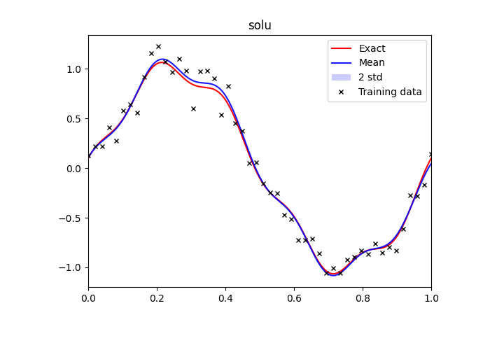
(b) FF_MBPINN_SGD

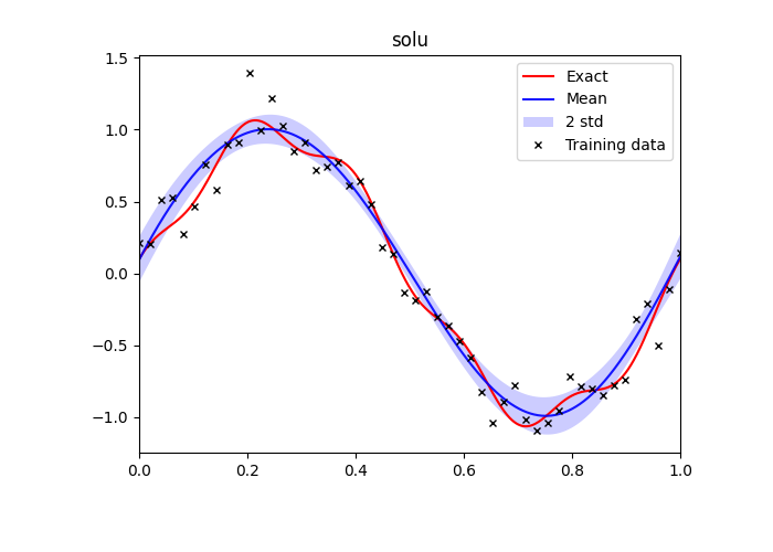
(c) clasical BPINN_HMC

Figure 3: Visualization of the solution of three different networks when the noise level is 0.1 for Example 1.

From the analysis of the Table 2 and Figure 3, it is evident that the MBPINN_SGD method offers several advantages over the other methods.

Example 2.

We consider the following two-dimensional multi-scale elliptic problem with two scale components in $\Omega=[-1,1]\times[-1,1]$.

$$\begin{cases}-\text{div}\left(a(x,y)\nabla u(x,y)\right)=f(x,y)\\ u(0,0)=u(1,0)=u(0,1)=u(1,1)=0.\end{cases}$$

where div denotes the divergence operator and $a(x,y)=\cos(3\pi x)\sin(5\pi y)$. We impose the exact solution

$$u(x,y)=\sin(\pi x)\sin(\pi y)+0.2\sin(5\pi x)\sin(5\pi y),$$

such that $f(x)$ can be obtained by direct computation.

Table 3: REL of different method to solve Example 2 for various noise level.

		0.005	0.001	0.0005	0.0001	0.00005	0.00001
	BPINN_HMC	—	—	—	—	—	1.617
	FF_MBPINN_HMC	—	—	—	—	—	—
0.05	FF_MBPINN_SGD	0.0065	0.0043	0.0028	0.0023	0.0035	0.2037
	2FF_MBPINN_HMC	—	—	—	—	—	—
	2FF_MBPINN_SGD	0.0074	0.0020	0.0034	0.0024	0.0069	0.0244
	BPINN_HMC	—	—	—	—	—	0.9654
	FF_MBPINN_HMC	—	—	—	—	—	0.0064
0.1	FF_MBPINN_SGD	0.0042	0.0154	0.0026	0.0062	0.0036	0.3279
	2FF_MBPINN_HMC	—	—	—	—	—	0.0073
	2FF_MBPINN_SGD	0.0051	0.0052	0.0045	0.0023	0.0024	0.1090

We solve the above smooth Poisson problem by employing the aforementioned five methods with solvers having two hidden layers, and each layer has 30 units. In this example, the 2500 random observations of force side in $\Omega$ are disturbed with mean-zero Gaussian distributed noise. In addition, the 800 random observations for boundary constraint on $\partial\Omega$ are also disturbed. Ansatzes expressed by DNN are used in BPINN_HMC to recover the solution simultaneously, and MscaleDNN with FFM pipelines are used in other methods. The $\Lambda$ of FF_MBPINN is set as 5 for the solution. The $\Lambda_{1}$ and $\Lambda_{2}$ of FF_MBPINN for solution are set as 1 and 5.

The result of this 2-dimensional multi-scale PDE problem (Table 3) shows that both FF_MBPINN_SGD and 2FF_MBPINN_SGD outperform the other methods, especially at smaller step sizes, where they consistently maintain lower REL. It is important to note that the BPINN-HMC method did run and provide a result at a step size of 0.00001 with an acceptance rate of 0, indicating that the result was entirely dependent on the initialization and, therefore, not valid. This low acceptance rate highlights a critical limitation of this method in such scenarios.

We also studied and visualized the performance of our proposed method for solving additional multi-scale and general problems in 1- to 3-dimensional spaces. These results further support our conclusions. Additionally, we examined the robustness of our method by varying key hyperparameters, such as the number of hidden layers and activation functions. Our experiments demonstrate that the method remains robust across different hyperparameter settings. All results from these studies are included in the Supplementary Materials.

Conclusion

The classical BPINN-HMC method faces significant challenges in practical applications, mainly due to the convergence issues of the HMC sampling method when solving general PDE problems, which are exacerbated as the complexity of the PDEs increases. Additionally, the basic setup of BPINN is somewhat simplistic and performs poorly with complex PDE problems. To address these issues simultaneously, we have proposed the MBPINN-SGD method, which has been tested and compared against BPINN-HMC on general Poisson and multi-scale elliptic problems across one- to three-dimensional spaces with noisy data. Our results demonstrate that MBPINN-SGD (1) is more robust than HMC, (2) incurs lower computational costs, and (3) offers greater flexibility in handling complex problems. However, when MBPINN is combined with HMC, the convergence issues of HMC worsen due to the inherent complexity of the Feature Fusion Module (FFM). This challenge warrants further investigation in the future.

Credit authorship contribution Statement

Yilong Hou: Methodology, Investigation, Validation, Writing - Original Draft. Xi’an Li: Conceptualization, Methodology, Investigation, Formal analysis, Validation, Writing - Review & Editing. Jinran Wu: Formal analysis, Writing - Review & Editing, Project administration.

References

- [Antil et al. 2021] Antil, H.; Elman, H. C.; Onwunta, A.; and Verma, D. 2021. Novel deep neural networks for solving bayesian statistical inverse. arXiv preprint arXiv:2102.03974.
- [Beck and Arnold 1977] Beck, J. V., and Arnold, K. J. 1977. Parameter estimation in engineering and science. James Beck.
- [Betancourt 2017] Betancourt, M. 2017. A conceptual introduction to hamiltonian monte carlo. arXiv preprint arXiv:1701.02434.
- [Blei, Kucukelbir, and McAuliffe 2017] Blei, D. M.; Kucukelbir, A.; and McAuliffe, J. D. 2017. Variational inference: A review for statisticians. Journal of the American statistical Association 112(518):859–877.
- [Ceccarelli 2019] Ceccarelli, D. 2019. Bayesian physics-informed neural networks for inverse uncertainty quantification problems in cardiac electrophysiology.
- [Engl, Hanke, and Neubauer 1996] Engl, H. W.; Hanke, M.; and Neubauer, A. 1996. Regularization of inverse problems, volume 375. Springer Science & Business Media.
- [Foong et al. 2019] Foong, A. Y.; Li, Y.; Hernández-Lobato, J. M.; and Turner, R. E. 2019. ’in-between’uncertainty in bayesian neural networks. arXiv preprint arXiv:1906.11537.
- [Iglesias, Law, and Stuart 2013] Iglesias, M. A.; Law, K. J.; and Stuart, A. M. 2013. Ensemble kalman methods for inverse problems. Inverse Problems 29(4):045001.
- [Jiang et al. 2022] Jiang, X.; Wanga, X.; Wena, Z.; Li, E.; and Wang, H. 2022. An e-pinn assisted practical uncertainty quantification for inverse problems. arXiv preprint arXiv:2209.10195.
- [Lee et al. 2017] Lee, J.; Bahri, Y.; Novak, R.; Schoenholz, S. S.; Pennington, J.; and Sohl-Dickstein, J. 2017. Deep neural networks as gaussian processes. arXiv preprint arXiv:1711.00165.
- [Li and Marzouk 2014] Li, J., and Marzouk, Y. M. 2014. Adaptive construction of surrogates for the bayesian solution of inverse problems. SIAM Journal on Scientific Computing 36(3):A1163–A1186.
- [Li et al. 2023] Li, S.; Xia, Y.; Liu, Y.; and Liao, Q. 2023. A deep domain decomposition method based on Fourier features. Journal of Computational and Applied Mathematics 423:114963.
- [Li, Grana, and Liu 2024] Li, P.; Grana, D.; and Liu, M. 2024. Bayesian neural network and bayesian physics-informed neural network via variational inference for seismic petrophysical inversion. Geophysics 89(6):1–46.
- [Li, Wang, and Yan 2023] Li, Y.; Wang, Y.; and Yan, L. 2023. Surrogate modeling for bayesian inverse problems based on physics-informed neural networks. Journal of Computational Physics 475:111841.
- [Li, Xu, and Zhang 2023] Li, X.-A.; Xu, Z.-Q. J.; and Zhang, L. 2023. Subspace decomposition based dnn algorithm for elliptic type multi-scale pdes. Journal of Computational Physics 488:112242.
- [Lin, Wang, and Zhang 2022] Lin, G.; Wang, Y.; and Zhang, Z. 2022. Multi-variance replica exchange sgmcmc for inverse and forward problems via bayesian pinn. Journal of Computational Physics 460:111173.
- [Linka et al. 2022] Linka, K.; Schäfer, A.; Meng, X.; Zou, Z.; Karniadakis, G. E.; and Kuhl, E. 2022. Bayesian physics informed neural networks for real-world nonlinear dynamical systems. Computer Methods in Applied Mechanics and Engineering 402:115346.
- [Meng et al. 2022] Meng, X.; Yang, L.; Mao, Z.; del Águila Ferrandis, J.; and Karniadakis, G. E. 2022. Learning functional priors and posteriors from data and physics. Journal of Computational Physics 457:111073.
- [Neal 2012a] Neal, R. M. 2012a. Bayesian learning for neural networks, volume 118. Springer Science & Business Media.
- [Neal 2012b] Neal, R. M. 2012b. Mcmc using hamiltonian dynamics. arXiv preprint arXiv:1206.1901.
- [Pensoneault and Zhu 2024] Pensoneault, A., and Zhu, X. 2024. Efficient bayesian physics informed neural networks for inverse problems via ensemble kalman inversion. Journal of Computational Physics 508:113006.
- [Perez et al. 2023] Perez, S.; Maddu, S.; Sbalzarini, I. F.; and Poncet, P. 2023. Adaptive weighting of bayesian physics informed neural networks for multitask and multiscale forward and inverse problems. Journal of Computational Physics 491:112342.
- [Rahaman et al. 2019] Rahaman, N.; Arpit, D.; Baratin, A.; Draxler, F.; Lin, M.; Hamprecht, F. A.; Bengio, Y.; and Courville, A. 2019. On the spectral bias of deep neural networks. International Conference on Machine Learning.
- [Sun and Wang 2020] Sun, L., and Wang, J.-X. 2020. Physics-constrained bayesian neural network for fluid flow reconstruction with sparse and noisy data. Theoretical and Applied Mechanics Letters 10(3):161–169.
- [Tancik et al. 2020] Tancik, M.; Srinivasan, P.; Mildenhall, B.; Fridovich-Keil, S.; Raghavan, N.; Singhal, U.; Ramamoorthi, R.; Barron, J.; and Ng, R. 2020. Fourier features let networks learn high frequency functions in low dimensional domains. Advances in Neural Information Processing Systems 33:7537–7547.
- [Wang and Zabaras 2004] Wang, J., and Zabaras, N. 2004. Hierarchical bayesian models for inverse problems in heat conduction. Inverse Problems 21(1):183.
- [Wang, Wang, and Perdikaris 2021] Wang, S.; Wang, H.; and Perdikaris, P. 2021. On the eigenvector bias of Fourier feature networks: From regression to solving multi-scale PDEs with physics-informed neural networks. Computer Methods in Applied Mechanics and Engineering 384:113938.
- [Woodbury 2002] Woodbury, K. A. 2002. Inverse engineering handbook. Crc press.
- [Xu et al. 2020] Xu, Z.-Q. J.; Zhang, Y.; Luo, T.; Xiao, Y.; and Ma, Z. 2020. Frequency principle: Fourier analysis sheds light on deep neural networks. Communications in Computational Physics 28(5):1746–1767.
- [Yang and Foster 2022] Yang, M., and Foster, J. T. 2022. Multi-output physics-informed neural networks for forward and inverse pde problems with uncertainties. Computer Methods in Applied Mechanics and Engineering 402:115041.
- [Yang, Meng, and Karniadakis 2021] Yang, L.; Meng, X.; and Karniadakis, G. E. 2021. B-pinns: Bayesian physics-informed neural networks for forward and inverse pde problems with noisy data. Journal of Computational Physics 425:109913.
- [Yao et al. 2019] Yao, J.; Pan, W.; Ghosh, S.; and Doshi-Velez, F. 2019. Quality of uncertainty quantification for bayesian neural network inference. arXiv preprint arXiv:1906.09686.