Surface spectroscopy and surface-bulk hybridization of Weyl semimetals
Abstract
Weyl semimetal showing open-arc surface states is a prominent example of topological quantum matter in three dimensions. With the bulk-boundary correspondence present, nontrivial surface-bulk hybridization is inevitable but less understood. Spectroscopies have been often limited to verifying the existence of surface Fermi arcs, whereas its spectral shape related to the hybridization profile in energy-momentum space is not well studied. We present an exactly solvable formalism at the surface for a wide range of prototypical Weyl semimetals. The resonant surface state and the bulk influence coexist as a surface-bulk hybrid and are treated in a unified manner. Directly accessible to angle-resolved photoemission spectroscopy, we analytically reveal universal information about the system obtained from the spectroscopy of resonant topological states. We systematically find inhomogeneous and anisotropic singular responses around the surface-bulk merging borderline crossing Weyl points, highlighting its critical role in the Weyl topology. The response in scanning tunneling spectroscopy is also discussed. The results will provide much-needed insight into the surface-bulk-coupled physical properties and guide in-depth spectroscopic investigation of the nontrivial hybrid in many topological semimetal materials.
Significance statement
Weyl semimetal is an epitome of frontier topological quantum materials. Its surface property accessible to photoemission measurements is important and contains rich information about the system. Lacking analysis of the inherent three-dimensional surface-bulk hybrid nature, investigations are often limited to verifying the existence of surface states and miss the hybridization aspect of general bulk-boundary correspondence. Based on an exactly solvable formalism consistently treating the surface and bulk states, we reveal the missing mathematical structure of the surface-bulk hybrid and the hidden information about the topological surface state; singular spectroscopic responses of the surface-bulk merging are highlighted. This underscores the importance of appreciating the intricate surface-bulk hybridization in quantum materials, paving the way for exploring such unique features.
Introduction
Topological quantum materials, characteristically accompanied by nontrivial topological states at the boundary, are an important frontier of condensed matter physics. Intriguing physical properties are often closely related to the principle of bulk-boundary correspondence and the boundary states. An epitome in three dimensions (3D) is the Weyl semimetal (WSM), which is significantly beyond an extension of the two-dimensional (2D) Dirac physics[1, 2, 3, 4, 5, 6, 7, 8, 9, 10, 11, 12, 13]. It shows Weyl points (WPs) with linear band crossings as momentum-space Dirac monopoles and the associated chiral anomaly effects[14, 15, 16, 17, 18, 19, 20, 21]. At its boundary, unusual open-arc surface states appear in the projected surface Brillouin zone (BZ)[22, 23, 24, 12, 25, 13]. However, such Fermi arc surface states cannot be separated from the bulk at will, e.g., in transport measurements, because they interplay to form an organic whole and hence contribute together. For instance, unique quantum oscillations and quantum Hall effects originate from the Weyl orbit combining arc and bulk states[26, 27, 28, 29, 30, 31, 32]. An important question arises: what are the mathematical structure and physical effects of the inherent 3D surface-bulk hybrid in WSMs?
How the boundary and bulk are nontrivially connected and hybridized is a less clear but indispensable aspect of the general principle of bulk-boundary correspondence. WSMs provide an ideal platform for such investigation because their 2D surfaces are open to many experimental probes. However, spectroscopy has been often limited to merely verifying the existence of surface states and overlooked the bulk-boundary hybrid and its nontrivial energy-momentum profile. Such information actually lies in the neighborhood of the surface and hides rich information about the whole system, crucial for studying further optical responses, transport and magnetic properties[33, 34, 35, 36, 25]. It should be naturally detectable by contemporary spectroscopies, e.g., the angle-resolved photoemission spectroscopy (ARPES) that resolves the important momentum dependence and the scanning tunneling spectroscopy (STS) that encodes the density of states in the tunneling I-V characteristics[37, 38, 39, 40]. Photoemission is presumably more tunable between surface or bulk sensitive via the penetration depth of variable photon energy, which thus can accommodate sensitively the effect of surface-bulk hybrid[41, 42]. Further equipped with spin resolution, these techniques can extract information inherent to the spin channel and magnetism as demonstrated experimentally[43, 44, 37, 38, 45, 46].
To this end, we present a general formalism for a wide range of typical WSMs (in terms of symmetry, number of WPs, and type of Weyl fermion) with an exact solution near the surface. The consistently unified surface state and bulk influence substantially broaden the physical reach. Targeting surface ARPES measurements, we find that the surface resonance signal contains much more information about the whole system than usually deemed, hidden but comprehensively encoded in its shape and intensity profile. A byproduct is finding unequal numbers of Fermi arcs and WP pairs, contrary to the common belief. Revealing the remarkable structure of surface-bulk hybrid, highly anisotropic singular responses near the loop-like surface-bulk merging borderline in the energy-momentum space are found accompanied by anomalous inverse square root scaling behavior. They provide a concrete prediction and picture of the borderline crucially mediating the surface-bulk hybridization, which serves as a critical transition boundary between surface and bulk effects, together with its own special edge at WPs. Due to the spin-polarized surface state, spin-resolved STS measurement can also achieve a separation of the bulk and surface tunneling contributions.
Results
Model and effective surface Green’s function
We consider a two-band Hamiltonian that breaks both the time-reversal and inversion symmetries
| (1) |
With appropriate parameter ranges, it gives a minimal pair of WPs aligned along the -direction as shown in Fig. 1(A) and at the energy . Finite break the particle-hole symmetry and add extra spin-independent dispersion in the -plane surface of our main interest; especially accounts for the realistic Fermi arcs with finite curvature, which is common in real materials and crucial, e.g., to many phenomena involving Weyl orbits. We show how this Hamiltonian is formulated and related to more general cases in Supplemental Information (SI) Sec. I. Also discussed later, most other types of WSMs with different symmetries and more WPs can be treated.

The surface effective Green’s function can be analytically obtained by considering a sample semi-infinite in the -direction. The Hamiltonian of the top surface, if decoupled from the bulk, is given by (summation over is henceforth understood) , where . We use to denote -dependence in the surface BZ for simplicity, which is our main focus. The whole system is then cast in a recursive form of coupled to neighboring layers. With the shorthand notation for generic complex frequency and , we obtain two exact solutions labelled by for the surface Green’s function (Methods)
| (2) |
where
| (3) |
depends on the choice of with
| (4) |
and . Momentum and energy dependence is henceforth suppressed for brevity. This solution is found by effectively integrating out the bulk degrees of freedom and the surface effective Green’s function will encode the full information of the original WSM system. A related approach via integrating the bulk has been applied to mesoscopic transport calculation and quantum oscillation under magnetic field[47, 28].
Spectral function

The information most relevant to spectroscopy can be extracted from the spectral function of Green’s function in (2). It is given by
| (5) |
where the retarded Green’s function , leading to the charge () and three spin () channels
| (6) |
In real systems, may signify the phenomenological strength of possible relaxation mechanisms, e.g., disorder, phonon scattering, electron correlation, etc. ARPES without spin resolution measures only while spin-resolved ARPES can extract each of with spin-polarized photoelectron detectors. To understand its physical meaning, it is crucial to know how in (3) should be chosen, which turns out to be a nontrivial issue because of (4) is not necessarily always positive. It is, however, remarkable to note that the above definition of spectral function holds in general regardless of the sign of under the square root because Green’s functions can generally be complex.
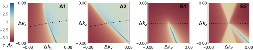
We plot the above spectral function in Fig. 2. Exemplified in Fig. 2(A1,B1), both the topological surface state and the influence from the bulk states are unified in and hence in ; the surface state eventually ends and merges into the bulk at a certain borderline in the energy-momentum space. To facilitate and guide the discussion, we point out three crucial aspects of the key quantity :
-
•
The sign of determines in the energy-momentum space the boundary between bulk contribution () and the region admissible to surface state ();
-
•
The borderline of surface state entails , where the surface state merges into the bulk states;
-
•
The choice of has to be determined physically according to the positivity of the charge channel spectral function , because it directly corresponds to the density of states.
Henceforth, when the sign of a certain quantity is concerned, complex frequency substituted by real is understood.
Surface resonance spectroscopy
We first find the states on-shell at the surface, i.e., the topological surface state. As long as for some energy-momentum region, the analytic continuation in (6) matters only in the denominator and gives (Methods)
| (7) |
When is finite, this readily implies the surface state dispersion relation
| (8) |
which mainly accounts for the circulating chiral states on the top surface, and is modified by the extra dispersions in the 2D surface BZ. As aforementioned and shown in Fig. 1(B2), finite bends the Fermi arc towards -direction to make it curved, otherwise the arc becomes a straight line. This is also consistent with earlier low-energy approximate solutions for simpler models[48, 49, 50]. Furthermore, the fact that only are finite and identical implies a locking between the charge and spin- channels; we also find the surface state entirely polarized in spin-. Such a locking and spinful feature is directly visible in Fig. 2, where the surface band appears identically in the charge and channel.
The resonance at the surface state (henceforth denoted by index ‘ss’) band (8) immediately leads to the relation and with
| (9) |
where and similarly for others. Here, generally satisfies the assumption of (7) self-consistently except for the special case . Thus, defines a momentum-space borderline of the surface state, i.e.,
| (10) |
which forms a loop that touches the two WPs projected in the 2D BZ, as shown in Fig. 1(B1). To have a nonvanishing spectral weight of the surface state in (7), needs to be finite and negative such that as aforementioned. Inside the borderline, i.e., within the constraint momentum-space region
| (11) |
the solution is chosen and one finds
| (12) |
where . Hence, (11) gives the physically allowed region in the 2D momentum space, within which the surface band (8) is defined. Outside this region one has and the only nonvanishing choice leads to unphysical , we thus still have and hence
| (13) |
which is physically expected beyond the surface state constraint and outside the bulk continuum.

It is intriguing to note that the momentum dependence of the resonance in (12) can be measured from the intensity in both charge and spin channels of ARPES, which encodes the information of the surface state constraint function or the Hamiltonian components . Such information is complementary to the surface band dispersion (8), which involves only and is measured through the surface band shape in ARPES as determined by the -function in (12). Therefore, from the resonance intensity and the band shape , most information of the bulk WSM system can be extracted by merely inspecting surface resonance (12), realizing an intriguing holography-like situation. For instance, as shown in Fig. 3, since ARPES measures photoemission intensity of occupied bands, at different chemical potentials tunable via gate voltage control, the Fermi arc in the 2D BZ traverses across the constraint region (11), and serves as a tomography of the surface resonance of the WSM. Here, we only exemplify the behavior of one particular surface. In experiments, different crystalline surfaces can be similarly measured, which will extract more complete information about the constraint and the Hamiltonian, including the anisotropy of the system. In other WSM systems where the surface carries more complex spin structures, in-plane can also supply further information.
In addition, with such a direct characterization of the surface state, we are able to point out yet another important but often overlooked phenomenon: the numbers of Fermi arcs and WP pairs are not necessarily identical. The common belief of a one-to-one correspondence between them assumes that an energy plane cuts a surface state continuum and gives an arc. In contrast, the constraint region (11) may not be simply connected. As shown in Fig. 1(C1,C2) for a minimal noncentrosymmetric model with two WP pairs (SI Sec. II), it can generally be multiply connected with inner holes, then the isoenergy curve is disconnected once it passes a hole, i.e., a forbidden region, even if the Fermi energy is at WPs. This leads to more Fermi arcs for one WP pair, depending on and also the hole position. In experiments, discretion is necessary when identifying or counting WPs from arc spectroscopy; instead, knowledge of the constraint region would be helpful. A hole, i.e., an inner boundary of the constraint region, is not fundamentally different from the usual outer boundary where arcs end; both are merging borderlines from surface to bulk and our later discussion applies equally well. For instance, an inner hole borderline can also pass WPs as the outer one does. The above phenomenon of excess Fermi arcs is very general and can appear in many other WSMs. In fact, based on the present formalism applied to WSMs with multiple WP pairs, we can accurately analyze more generic but unconventional properties of the projected surface connection pattern (SI Sec. IV). Strongly affected by the shape of constraint region and surface state energy surface and especially tuned by , the naive association of a Fermi arc with a WP pair is often not the case.
Signatures from bulk continuum
Since Green’s function (2) has the bulk beneath the top surface integrated out, it should have the bulk state contribution included as well, albeit in an off-resonance manner. As aforementioned, away from the energy-momentum space region that admits possible surface state, we do not necessarily have . Rewriting (4) as with , we require and generally find two disconnected regions in the energy-momentum space for
| (14) |
They exactly correspond to the projection of bulk states onto the surface, which manifests as conduction and valence bands. Within such continuum regions, of (3) acquires a finite imaginary part even before the analytic continuation and dominates the spectral function (5); such a contribution is thus off-resonance, i.e., finite and not peaked as -functions as the surface state. Therefore, should signify the band edges of the bulk states measured from . We exemplify such band edges in Fig. 2(A1,B1). In fact, we note from Hamiltonian (1) that the bulk eigenenergy (measured from ) squared reads
| (15) |
where is the polar angle of the coordinate . Its two extrema are exactly the foregoing . When such band edges accidentally touch each other, the effective Green’s function (2) will become singular (SI Sec. V).
It is noteworthy that the choice of solution branches in (2) becomes in general more complicated outside the surface resonance, including the bulk continuum and the merging borderline. However, one can reach an exceptionally simple criterion at any and , not limited to surface or bulk contribution (Methods): find the choice of that maximizes . This is how all the spectral functions are evaluated throughout this study.
In Fig. 2, we indeed observe the projection of bulk conduction and valence bands in the surface BZ and they are connected through the surface band in between. In Fig. 3(A-C), the Fermi arc similarly connects two bulk Weyl cones separated along direction; the bulk state is itself connected at energy higher than the WP in Fig. 3(D,E), which is due to the distortion from and consistent with Fig. 2(B1). Also, as aforementioned, the spectral intensity of the projected bulk bands remains independent from in (6), in contrast to the surface resonance. From (2) and (6), we know that and are finite only when for the bulk continuum region, so they all vanish for the surface state resonance as discussed previously. An immediate implication is that the in-plane spin spectral weight only appears in the bulk continuum and respectively follows the profile of , e.g., both and changes sign at , as we observe in Fig. 2. seemingly suggests , which does not accurately hold in Fig. 2(A4) although the trend remains in gross. This is because such bulk symmetry, under surface projection, will be distorted, as exemplified by the chiral surface state obviously asymmetric for . In fact, if the opposite surface was included, the overall symmetry could be restored for the whole sample.
Singular behavior along merging borderline
We inspect how the surface state merges into the bulk and the behavior around the merging points, i.e., the borderline, which is a twofold restriction in the energy-momentum space as shown in Fig. 1(B,C): the loop-like border of the surface state constraint (10) in the surface BZ and the energy pinned to the corresponding surface band. Since except for the borderline, the entire surface band (8) at any in the whole surface BZ (dashed line in Fig. 2(A1,B1)), not limited to the constraint region (11), is separated from the bulk states (). Hence, they will tangentially touch each other at the borderline. The real surface state restricted by the constraint thus merges into the bulk continuum at the borderline, as shown in Fig. 2 and Fig. 3. Although the surface resonance is outside the bulk continuum, its residual influence, according to (2) and (6), enters and of the bulk continuum through the energy denominator (index ‘bs’ for bulk states)
| (16) |
This means stronger spectral weight in and if close to the full surface state dispersion of (8) regardless of the constraint, as seen in Fig. 2(A1,A4,B1,B4). This is physically understandable as the resonant surface spectral weight will not suddenly disappear but smear into the bulk continuum.
Approaching the merging borderline from the bulk continuum, both the nominator and denominator reduce to zero in (16), which becomes apparently undetermined. The similar happens in (7) or (12) from the surface resonance side as key quantities all approach zero. To reveal the singular behavior thereof for any approaching direction, we consider the expansion around the momentum and energy on the borderline respectively (denoted by index ‘bl’), i.e., . One can cast quantities in (3) up to the relevant orders in and
| (17) |
where all parameters like and rank-2 tensor are evaluated along the borderline and given in Methods. is the linear order term of , and with notation , we denote
| (18) |
While accounts for the leading linear effect in along almost the entire borderline, it vanishes at WPs as per the general model construction, hence the rest of quadratic terms will become important. With (17), the general spectral function around the entire borderline is
| (19) |
We visualize case for representative borderline points away from and at the WP in Fig. 4, where a type-II WSM case is exemplified in comparison when the velocity tilting is large enough to induce the Lifshitz transition[51] (SI Sec. VI). In Fig. 5, we additionally visualize the evolution and transition in the proximity of the merging borderline, in which the anomalous behavior across the merging along momentum axes manifests conspicuously.

We first approach the borderline along the surface state resonance. Following the earlier discussion of surface resonance spectroscopy, this sets in the first place in (17) and leads to . Now (19) becomes in the limit
| (20) |
The surface state constraint (11) also applies and defines the outward normal direction at the constraint region boundary, which is generally nonzero. Hence, its resonance intensity scales with the momentum normal to the borderline; exactly means that needs to be inward the constraint region to have finite signals.
(20) misses the continuum side and the generic off-resonance behavior outside the bulk continuum. With deviation from the surface state resonance, the full form (19) captures the correct behavior as shown in Fig. 4, where especially in becomes the leading linear contribution away from WPs. If only this leading effect is concerned, the formula reduces to
| (21) |
This formula determines the local merging configuration, including whether the borderline is approached from the bulk continuum or the surface state region near the conduction or the valence band (see Methods). Besides, along the borderline it exhibits a singularity scaled as with . Without much loss of generality, we will refer to it by -singularity. Therefore remarkably, the borderline is a set of singular branch points with unconventional inverse square root divergence , in contrast to the usual -function due to a simple pole divergence . It resolves the foregoing undeterminedness in any direction, where the spectral weight changes between resonant -function divergence (surface-state side), -singularity (borderline), and finite (bulk side). Accordingly in Fig. 5(A), the blue, yellow, and green signals approach the merging point (red signal) from the surface side while the associated surface state resonance is weakened and transitions to the anomalously peaked resonance at merging; further into the bulk side, such a -divergence changes to the smooth purple and brown signals. This elucidates what happens in Fig. 3(A,B) and Fig. 4(A) near the merging. The borderline forms a set of critical transition points of the spectral signal in ARPES, regardless of the approaching direction in energy-momentum space. With finite relaxation strength , the signal variation could become a smoother crossover, but the scaling behavior, including that of the linewidth, bears the same transition.
Around WPs, is fully quadratic in deviations and (19) takes the form
| (22) |
where and . This formula fully captures the merging configuration around WPs, especially the distinction between type-I and type-II cases, as shown in Fig. 4(B), is directly related to the principal values of the tensor (see Methods). Approaching the WPs, (22) gives with chosen. This singles out the WP as a unique removable singularity of spectral weight as shown in Fig. 4(B), which purely depends on the hopping amplitude and does not diverge with vanishing . In Fig. 5(B), we observe that the bulk gap closes smoothly and reopens; more specifically, it shrinks to zero while the intensity of surface state resonance is weakened to zero upon reaching the merging point (WP), where it transitions to the red finite WP signal. The surface states entirely end at WPs and WPs simultaneously belong to the bulk continuum; this physically explains why the WP signal eventually does not diverge as surface states do. It thus is distinct from the foregoing surface-borderline-bulk transition and instead admits either a surface-bulk transition as in Fig. 5(B) (from -function divergence to finite) or a borderline-bulk transition (from -divergence to finite), depending on whether the WP is approached from the majority of surface states or along the borderline. Note that the intensity of -singularity decreases with the distance from the WP along the borderline.
These discussions reveal the strong inhomogeneity along the borderline in terms of both the near-merging behavior and the singularities themselves, reflecting a fundamental aspect of the topology generated between WPs in a WSM. While the borderline can be viewed as a special edge curve of the surface state where distinct phenomena occur, there also exist WPs as the special points on the borderline. The surface/bulk distinction plays an important role and one can approach the borderline from either side. On each side, it exhibits nontrivial energy-dependence and highly anisotropic angle -dependence for the entire borderline. Such information provides important profiling of the WSM system, as reflected in Fig. 4 and Fig. 5, and can be measured in ARPES directly, e.g., through inspecting the endpoint behavior of Fermi arcs in Fig. 3.
STS measurement

STS measurement finds differential conductance from varying the bias voltage of the (spin-polarized) tip. It is able to reconstruct the local density of the electronic states and is directly related to the spectral function (6) integrated over momentum, i.e., with the area of the surface BZ. An extra merit of STS is that it can probe both occupied and empty states by simply changing the sign of bias voltage. This is, however, achievable in ARPES by directly tuning the chemical potential or with pump-probe ARPES[52]. In the presence of impurities, quasiparticle interference patterns of STS related to spatially dependent can also detect the surface Fermi contour[53, 33, 42, 54, 55].
Fig. 6 shows the integrated spectral weight in charge and spin channels. The asymmetry with respect to the WP energy is due to the broken particle-hole symmetry in (1). By virtue of our analytical solution that physically identifies the meaning of the key quantity , the surface and bulk contributions can also be clearly separated as and . Corroborating with our earlier discussion, only and are finite while comes from all channels. The van Hove singularity in originates from the lowest energy part of the surface band in Fig. 1(B2), which can become relatively flat as the band minimum. This particularly happens when the Weyl vector, the separation vector between WPs, is long such that the constraint region covers the surface band minimum. Therefore, it can be used as a phenomenon for estimating the Weyl vector scale important in experiments. Near the WP energy, bulk spectral weight vanishes in every channel while that from the surface state dominantly contributes in a way that manifests the locking between the charge and spin- channels, which can be used as direct experimental evidence for identifying topological arc states. Besides directly accessing charge and spin channels in either ARPES or STS, one can also measure different surfaces of the sample that may bear arc states or not, from which the unique surface contribution can be clearly identified in comparison and even separated if the anisotropy between those surfaces is not too large.
Discussion and Summary
The main WSM model we focused on can be realized in its own right in minimal magnetic Weyl materials and particularly also captures the surface spin polarization effect directly observable in spin-resolved ARPES and STS. Such discussion singles out the most important physical properties in general magnetic or noncentrosymmetric Weyl materials even with multiple pairs of WPs, since the pairwise connection of projected WPs on a surface is a common and distinguishing feature. In fact, the formalism is general enough to account for more interesting cases, e.g., the time-reversal-breaking WSM with more WP pairs and the inversion-breaking WSM with more pairs such as the one shown in Fig. 1(C1,C2) and WPs not at the same energy (SI Secs. II and III). Importantly, the main features discussed remain intact, despite the distinct shape of the surface state. For noncentrosymmetric Weyl materials, the number of WP pairs has been reduced from twelve in TaAs to four[51, 56, 42, 57] and the minimal two[58, 52]; increasingly many magnetic Weyl materials also appear in experiments and theoretical predictions, even with two or the minimal one pair of WPs[59, 60, 12, 25, 13].
As we have already exemplified, all the analysis equally applies to type-II WSMs and the formulae and conclusions are fully general (SI Sec. VI). For example, an immediate observation is that although the surface band dispersion (8) will be strongly tilted by , the surface state constraint region (11) remains intact. Last but not least, the Dirac semimetal case shares similar physics as the signal will be effectively contributed by, e.g., one more pair of WPs, which can be readily captured by adding an extra chirality-reversed copy of the model in our discussion and none of the essential conclusions will change.
Based on a formalism of exactly solved WSM models at the surface, we present a unifying treatment of the topological surface state and the bulk continuum and reveal the crucial hybridization aspect of the bulk-boundary correspondence. This strongly broadens the physical access and enables a comprehensive analysis of the spectroscopic effects of the surface inseparable from the bulk. Important but often overlooked information about the bulk Hamiltonian and surface constraint can be revealed by surface spectroscopy. Unconventional transitions at the surface-bulk merging borderline are found via a systematic analysis of the highly anisotropic singular responses in the energy-momentum space. The fully analytical account and the general prediction will deepen our understanding of topological semimetals from their 3D surface-bulk hybrid nature and push forward the frontier of spectroscopy experiments on topological systems.
Methods
Solution method of model Hamiltonian
Here we sketch the method of solving the surface Green’s function. For a sample semi-infinite in the -direction, the Hamiltonian (1) can be given in a recursive form. Contiguous -layers start from the top surface and serve as the matrix indices
| (23) |
where , given in the main text, is the Hamiltonian of the top layer decoupled from the bulk. Also, the inter--layer coupling takes the form with and . We focus on the Green’s function of the top -surface with generic complex frequency and the original Green’s function of . Making use of the recursive property of (23), the self-energy of for the top surface is given by
| (24) |
When we have the bare Green’s function of as , the exact Dyson equation reads
| (25) |
which is an equation of in the effective surface Green’s function . Intuitively, the foregoing form of interlayer coupling given by hides the information of , which is ‘squeezed’ but encoded in the surface . Hence, one finds the intriguing structure of (2), especially the importance of that appears in the energy denominator only for . In SI Sec. I, we discuss in more detail how such a formalism can be applied to more general Hamiltonians.
We in general face the issue of the choice of in calculating (5), which is now extra complicated by the inevitable branch cut of square root in (3). Firstly, it is a convenient choice to place the branch cut at ; to account properly for the surface state case of , should be avoided, otherwise, it would cause an unphysical exchange between the shaded surface state constraint region in Fig. 1(B1) and its complement. Secondly, as aforementioned, can be fixed by the positive-definiteness of the charge channel spectral weight . Since the off-resonance bulk contribution is purely coming from the imaginary part , i.e., in (3), only one makes and hence naturally determines the choice. Slightly away from the surface state resonance and when the analytic continuation in (6) practically uses a finite , such uniqueness of for positive may not hold everywhere, e.g., around the borderline of the constraint region where the surface state merges into the bulk states; this, however, can be resolved by noting that the spectral function varies smoothly away from the exact surface state resonance in (12). With these considerations combined, we reach the simple but general criterion at any and : find the choice of that maximizes .
Surface state resonance and behavior near the borderline
According to (2), the effect of surface state resonance can only enter the component below of the spectral function via the substitution
| (26) |
where only the second part with matters and gives the Lorentzian structure, because outside the bulk continuum. We thus target the charge-spin-locked in the following. In the general on surface state resonance, we use (9) and separate out the contribution due to relaxation
| (27) |
where . When , i.e., away from the surface-bulk borderline, we have
| (28) |
where we retain the leading contribution of . Inside the surface state constraint region (11), is contributed only by because the second part in the second line of (28) is at least in its real part; this indicates the choice aforementioned and we obtain (12) in the main text, where is from the resonance suggested in (26).
To study the property in the vicinity of the borderline between the surface state and the bulk, it suffices to focus on according to (2). Importantly, the full effect up to the quadratic order in is relevant to our discussion. We separate using (9). Up to the leading order, we firstly find , where , dependent on that determines the constraint region (11), defines the normal direction at the boundary of the constraint region and is in general finite along the entire borderline. Secondly, we have with
| (29) |
where , , , and the rank-2 Hessian tensor with . Then we have
| (30) |
up to the linear order with , which suffices for our purpose. This leads to
| (31) |
with , , and . In the vicinity of WPs, (30) and (31) become
| (32) |
with and all parameters evaluated at the WPs. Note that we use primed notation explicitly for parameters defined for generic borderline points, which is omitted in (17) for brevity. With these definitions, (2) gives
| (33) |
Besides the unimportant -linear term, its leading order is generally nonlinear in and higher order than , which is negligible compared to below. Hence, we have identical within the leading order around the entire borderline and can obtain (19) and what follows.
Determine the merging configuration
Given the crucial role of in (19), (21), and (22), it is clarifying to understand its physical meaning, which exactly determines the local merging configuration. Along the borderline except WPs, regarding (21), is transparent per the surface/bulk distinction of : changing the signs of , i.e., deviating in opposite directions away from the borderline, switches between surface and bulk contributions. For instance, setting , one finds . Since is the chiral part of the surface band (8), means the upper point merging into the bulk conduction band, then is respectively above (bulk continuum) or below (surface state region) the merging point; similarly accounts for merging into the valence band. Setting , one finds . The factor fixes the local chirality, i.e., the sign of the slope, of surface dispersion at the merging point: if it is increasing, say, with respect to , and enters the conduction band (), its left () must be in the bulk continuum with while the right () is outside. These are all observed in, e.g., Fig. 2(A) and also Fig. S10(A) for the type-II case. Therefore, compared to deviation involving , one has an extra sign of along some direction; together they fully determine the local merging configuration.
In the very vicinity of the WPs, as shown in (22), now any causes , reflecting that pure energy deviation from a WP always enters the bulk Weyl cone however tilted, as shown in, e.g., the type-II Fig. S10(B). When , determines the sign of and is positive-definite unless the velocity tilting is large enough. This directly corresponds to the distinction between type-I and type-II WSMs as shown in Fig. 4(B), since with a negative eigenvalue means along a certain range of direction, i.e., such momentum deviation enters immediately the bulk electron/hole pockets once it leaves the WP. For the present model with , the two eigenvalues of the principal axes of are respectively along . Hence, large and deviation can enter the bulk continuum while does not in the spectroscopy.
Acknowledgements.
This work was supported by JSPS KAKENHI (No. 18H03676) and JST CREST (No. JPMJCR1874). X.-X.Z. was partially supported by RIKEN Special Postdoctoral Researcher Program.References
- Volovik [1987] G. E. Volovik, J. Phys. C: Solid State Phys. 20, L83 (1987).
- Murakami [2007] S. Murakami, New J. Phys. 9, 356 (2007).
- Wan et al. [2011] X. Wan, A. M. Turner, A. Vishwanath, and S. Y. Savrasov, Phys. Rev. B 83, 205101 (2011).
- Burkov and Balents [2011] A. A. Burkov and L. Balents, Phys. Rev. Lett. 107, 127205 (2011).
- Xu et al. [2011] G. Xu, H. Weng, Z. Wang, X. Dai, and Z. Fang, Phys. Rev. Lett. 107, 186806 (2011).
- Weng et al. [2015] H. Weng, C. Fang, Z. Fang, B. A. Bernevig, and X. Dai, Phys. Rev. X 5, 011029 (2015).
- Huang et al. [2015] S.-M. Huang, S.-Y. Xu, I. Belopolski, C.-C. Lee, G. Chang, B. Wang, N. Alidoust, G. Bian, M. Neupane, C. Zhang, S. Jia, A. Bansil, H. Lin, and M. Z. Hasan, Nat. Commun. 6, 7373 (2015).
- Xu et al. [2015] S.-Y. Xu, I. Belopolski, N. Alidoust, M. Neupane, G. Bian, C. Zhang, R. Sankar, G. Chang, Z. Yuan, C.-C. Lee, S.-M. Huang, H. Zheng, J. Ma, D. S. Sanchez, B. Wang, A. Bansil, F. Chou, P. P. Shibayev, H. Lin, S. Jia, and M. Z. Hasan, Science 349, 613 (2015).
- Lv et al. [2015a] B. Q. Lv, H. M. Weng, B. B. Fu, X. P. Wang, H. Miao, J. Ma, P. Richard, X. C. Huang, L. X. Zhao, G. F. Chen, Z. Fang, X. Dai, T. Qian, and H. Ding, Phys. Rev. X 5, 031013 (2015a).
- Lv et al. [2015b] B. Q. Lv, N. Xu, H. M. Weng, J. Z. Ma, P. Richard, X. C. Huang, L. X. Zhao, G. F. Chen, C. E. Matt, F. Bisti, V. N. Strocov, J. Mesot, Z. Fang, X. Dai, T. Qian, M. Shi, and H. Ding, Nat. Phys. 11, 724 (2015b).
- Yang et al. [2015] L. X. Yang, Z. K. Liu, Y. Sun, H. Peng, H. F. Yang, T. Zhang, B. Zhou, Y. Zhang, Y. F. Guo, M. Rahn, D. Prabhakaran, Z. Hussain, S.-K. Mo, C. Felser, B. Yan, and Y. L. Chen, Nat. Phys. 11, 728 (2015).
- Armitage et al. [2018] N. P. Armitage, E. J. Mele, and A. Vishwanath, Rev. Mod. Phys. 90, 015001 (2018).
- Lv et al. [2021] B. Lv, T. Qian, and H. Ding, Reviews of Modern Physics 93, 025002 (2021).
- Nielsen and Ninomiya [1983] H. Nielsen and M. Ninomiya, Phys. Lett. B 130, 389 (1983).
- Son and Spivak [2013] D. T. Son and B. Z. Spivak, Phys. Rev. B 88, 104412 (2013).
- Burkov [2014] A. Burkov, Physical Review Letters 113, 247203 (2014).
- Li et al. [2016] Q. Li, D. E. Kharzeev, C. Zhang, Y. Huang, I. Pletikosić, A. V. Fedorov, R. D. Zhong, J. A. Schneeloch, G. D. Gu, and T. Valla, Nat. Phys. 12, 550 (2016).
- Xiong et al. [2015] J. Xiong, S. K. Kushwaha, T. Liang, J. W. Krizan, M. Hirschberger, W. Wang, R. J. Cava, and N. P. Ong, Science 350, 413 (2015).
- Shekhar et al. [2015] C. Shekhar, A. K. Nayak, Y. Sun, M. Schmidt, M. Nicklas, I. Leermakers, U. Zeitler, Y. Skourski, J. Wosnitza, Z. Liu, Y. Chen, W. Schnelle, H. Borrmann, Y. Grin, C. Felser, and B. Yan, Nat. Phys. 11, 645 (2015).
- Cheng et al. [2021] B. Cheng, T. Schumann, S. Stemmer, and N. P. Armitage, Science Advances 7, eabg0914 (2021).
- Ong and Liang [2021] N. P. Ong and S. Liang, Nature Reviews Physics 3, 394 (2021).
- Burkov [2016] A. A. Burkov, Nature Materials 15, 1145 (2016).
- Yan and Felser [2017] B. Yan and C. Felser, Annual Review of Condensed Matter Physics 8, 337 (2017).
- Burkov [2018] A. Burkov, Annual Review of Condensed Matter Physics 9, 359 (2018).
- Nagaosa et al. [2020] N. Nagaosa, T. Morimoto, and Y. Tokura, Nature Reviews Materials 5, 621 (2020).
- Potter et al. [2014] A. C. Potter, I. Kimchi, and A. Vishwanath, Nature Communications 5, 5161 (2014).
- Zhang et al. [2016a] Y. Zhang, D. Bulmash, P. Hosur, A. C. Potter, and A. Vishwanath, Scientific Reports 6, 23741 (2016a).
- Borchmann and Pereg-Barnea [2017] J. Borchmann and T. Pereg-Barnea, Phys. Rev. B 96, 125153 (2017).
- Wang et al. [2017] C. Wang, H.-P. Sun, H.-Z. Lu, and X. Xie, Physical Review Letters 119, 136806 (2017).
- Zhang et al. [2018] C. Zhang, Y. Zhang, X. Yuan, S. Lu, J. Zhang, A. Narayan, Y. Liu, H. Zhang, Z. Ni, R. Liu, E. S. Choi, A. Suslov, S. Sanvito, L. Pi, H.-Z. Lu, A. C. Potter, and F. Xiu, Nature 565, 331 (2018).
- Nishihaya et al. [2021] S. Nishihaya, M. Uchida, Y. Nakazawa, M. Kriener, Y. Taguchi, and M. Kawasaki, Nature Communications 12, 2572 (2021).
- Zhang et al. [2021] C. Zhang, Y. Zhang, H.-Z. Lu, X. C. Xie, and F. Xiu, Nature Reviews Physics 3, 660 (2021).
- Inoue et al. [2016] H. Inoue, A. Gyenis, Z. Wang, J. Li, S. W. Oh, S. Jiang, N. Ni, B. A. Bernevig, and A. Yazdani, Science 351, 1184 (2016).
- Gorbar et al. [2016] E. V. Gorbar, V. A. Miransky, I. A. Shovkovy, and P. O. Sukhachov, Physical Review B 93, 235127 (2016).
- Duan et al. [2018] H.-J. Duan, S.-H. Zheng, P.-H. Fu, R.-Q. Wang, J.-F. Liu, G.-H. Wang, and M. Yang, New Journal of Physics 20, 103008 (2018).
- Cheng et al. [2020] B. Cheng, N. Kanda, T. N. Ikeda, T. Matsuda, P. Xia, T. Schumann, S. Stemmer, J. Itatani, N. Armitage, and R. Matsunaga, Physical Review Letters 124, 117402 (2020).
- Lv et al. [2019] B. Lv, T. Qian, and H. Ding, Nature Reviews Physics 1, 609 (2019).
- Sobota et al. [2021] J. A. Sobota, Y. He, and Z.-X. Shen, Reviews of Modern Physics 93, 025006 (2021).
- Binnig and Rohrer [1987] G. Binnig and H. Rohrer, Reviews of Modern Physics 59, 615 (1987).
- Bonnell [2000] D. Bonnell, ed., Scanning Probe Microscopy and Spectroscopy, 2nd ed. (Wiley-VCH, New York, 2000).
- Petersen et al. [2000] L. Petersen, P. Hofmann, E. Plummer, and F. Besenbacher, Journal of Electron Spectroscopy and Related Phenomena 109, 97 (2000).
- Deng et al. [2016] K. Deng, G. Wan, P. Deng, K. Zhang, S. Ding, E. Wang, M. Yan, H. Huang, H. Zhang, Z. Xu, J. Denlinger, A. Fedorov, H. Yang, W. Duan, H. Yao, Y. Wu, S. Fan, H. Zhang, X. Chen, and S. Zhou, Nature Physics 12, 1105 (2016).
- Cacho et al. [2015] C. Cacho, A. Crepaldi, M. Battiato, J. Braun, F. Cilento, M. Zacchigna, M. C. Richter, O. Heckmann, E. Springate, Y. Liu, S. S. Dhesi, H. Berger, P. Bugnon, K. Held, M. Grioni, H. Ebert, K. Hricovini, J. Minár, and F. Parmigiani, Physical Review Letters 114, 097401 (2015).
- Jozwiak et al. [2016] C. Jozwiak, J. A. Sobota, K. Gotlieb, A. F. Kemper, C. R. Rotundu, R. J. Birgeneau, Z. Hussain, D.-H. Lee, Z.-X. Shen, and A. Lanzara, Nature Communications 7, 13143 (2016).
- Bode [2003] M. Bode, Reports on Progress in Physics 66, 523 (2003).
- Wiesendanger [2009] R. Wiesendanger, Reviews of Modern Physics 81, 1495 (2009).
- Lewenkopf and Mucciolo [2013] C. H. Lewenkopf and E. R. Mucciolo, J. Comput. Electron. 12, 203 (2013).
- Okugawa and Murakami [2014] R. Okugawa and S. Murakami, Phys. Rev. B 89, 235315 (2014).
- Zhang et al. [2016b] S.-B. Zhang, H.-Z. Lu, and S.-Q. Shen, New Journal of Physics 18, 053039 (2016b).
- Zhang and Nagaosa [2022] X.-X. Zhang and N. Nagaosa, Nano Letters 22, 3033 (2022).
- Soluyanov et al. [2015] A. A. Soluyanov, D. Gresch, Z. Wang, Q. Wu, M. Troyer, X. Dai, and B. A. Bernevig, Nature 527, 495 (2015).
- Belopolski et al. [2017] I. Belopolski, P. Yu, D. S. Sanchez, Y. Ishida, T.-R. Chang, S. S. Zhang, S.-Y. Xu, H. Zheng, G. Chang, G. Bian, H.-T. Jeng, T. Kondo, H. Lin, Z. Liu, S. Shin, and M. Z. Hasan, Nature Communications 8, 942 (2017).
- Chang et al. [2016] G. Chang, S.-Y. Xu, H. Zheng, C.-C. Lee, S.-M. Huang, I. Belopolski, D. S. Sanchez, G. Bian, N. Alidoust, T.-R. Chang, C.-H. Hsu, H.-T. Jeng, A. Bansil, H. Lin, and M. Z. Hasan, Physical Review Letters 116, 066601 (2016).
- Zheng et al. [2016] H. Zheng, G. Bian, G. Chang, H. Lu, S.-Y. Xu, G. Wang, T.-R. Chang, S. Zhang, I. Belopolski, N. Alidoust, D. S. Sanchez, F. Song, H.-T. Jeng, N. Yao, A. Bansil, S. Jia, H. Lin, and M. Z. Hasan, Physical Review Letters 117, 266804 (2016).
- Yuan et al. [2019] Q.-Q. Yuan, L. Zhou, Z.-C. Rao, S. Tian, W.-M. Zhao, C.-L. Xue, Y. Liu, T. Zhang, C.-Y. Tang, Z.-Q. Shi, Z.-Y. Jia, H. Weng, H. Ding, Y.-J. Sun, H. Lei, and S.-C. Li, Science Advances 5, eaaw9485 (2019).
- Ruan et al. [2016] J. Ruan, S.-K. Jian, D. Zhang, H. Yao, H. Zhang, S.-C. Zhang, and D. Xing, Physical Review Letters 116, 226801 (2016).
- Jiang et al. [2017] J. Jiang, Z. Liu, Y. Sun, H. Yang, C. Rajamathi, Y. Qi, L. Yang, C. Chen, H. Peng, C.-C. Hwang, S. Sun, S.-K. Mo, I. Vobornik, J. Fujii, S. Parkin, C. Felser, B. Yan, and Y. Chen, Nature Communications 8, 13973 (2017).
- Koepernik et al. [2016] K. Koepernik, D. Kasinathan, D. V. Efremov, S. Khim, S. Borisenko, B. Büchner, and J. van den Brink, Physical Review B 93, 201101 (2016).
- Nie et al. [2017] S. Nie, G. Xu, F. B. Prinz, and S. cheng Zhang, Proceedings of the National Academy of Sciences 114, 10596 (2017).
- Jin et al. [2017] Y. J. Jin, R. Wang, Z. J. Chen, J. Z. Zhao, Y. J. Zhao, and H. Xu, Physical Review B 96, 201102 (2017).
- Zhang and Nagaosa [2017] X.-X. Zhang and N. Nagaosa, Phys. Rev. B 95, 205143 (2017).
- Kim et al. [2016] K. W. Kim, W.-R. Lee, Y. B. Kim, and K. Park, Nature Communications 7, 13489 (2016).
Supplemental Information
for “”
Xiao-Xiao Zhang1,2 and Naoto Nagaosa2
1Wuhan National High Magnetic Field Center and School of Physics, Huazhong University of Science and Technology, Wuhan 430074, China
2RIKEN Center for Emergent Matter Science (CEMS), Wako, Saitama 351-0198, Japan
I Formulation of general model Hamiltonians
One can consider more general WSM Hamiltonians such as
| (S1) |
which also can bear two WPs at under the following condition: and . Following the same procedure outlined in Methods, one obtains with
| (S2) |
and , which is not immediately analytically tractable. We firstly notice that , which introduces extra spin-independent dispersion along , does not fundamentally affect the discussion of the sample with a surface normal to -axis and can be safely neglected; note that more important for the surface in -plane, which lead to the distortion of the surface state and especially the Fermi arc curvature, are included. We secondly put without much loss of generality, which insignificantly affects the Fermi velocity along and now serves as the coupling strength between the surface layer and the bulk. With these assumptions, the analytical solution can be obtained in essentially a similar way. In fact, such a type of solution mainly relies on making the hoppings in the normal direction simple, which is in our setting. On the other hand, there is basically no constraint for the in-plane directions: can be any function of and for instance, it is not limited to nearest neighbor hoppings as in Eq. (S1). Therefore, a large class of WSM Hamiltonians can be exactly treated similarly and on this more general basis, one can physically expect that those beyond such an analytical form also share similar properties.
II Noncentrosymmetric WSM


The Hamiltonian Eq. (1) in the main text breaks the time-reversal symmetry and is mainly considered to have a real spin degree of freedom. However, at the level of general model construction, Pauli matrices can either stand for a real spin or a pseudospin and our formalism does not depend on this choice. To consider inversion symmetry , for a real spin, the inversion operation makes ; for a pseudospin due to orbital degree of freedom, the inversion additionally has the unitary matrix operation, which we consider to be here. In this sense, Hamiltonian Eq. (1) in general breaks inversion symmetry, which can be easily seen from its asymmetric WP location with respect to inversion. For the pseudospin case, special makes it inversion symmetric. In any case, -breaking determines the minimal number of WP pair is one.
We can otherwise consider the -broken WSM but with preserved, which has a minimum of two pairs of WPs. To this end, we can study, for instance, the following model with
| (S3) |
which is also the model used in Fig. 1(C1,C2). It respects as a pseudospin model with the operation given by complex conjugation. The two pairs of WPs are located at with and independently. We restrict the range of to throughout the study. The -related monopole pair () and antimonopole pair () are the pairs; the monopole-antimonopole pairs for with given are connected by topological surface states with Fermi arcs.
In the same manner as the -broken model in the main text, we present for this WSM model the ARPES signal in Fig. S1, the surface state information in Fig. S2, and the Fermi arc spectroscopy in Fig. S3. The blue or red spots in the lower branch in Fig. S1(B1,B3,B4) also exemplify the discussion in Sec. V as they are slightly near the divergence. The absence of such spots in Fig. S1(B2) is because the Green’s function component exactly vanishes there as per the Hamiltonian.


Another -broken WSM model is[61]
| (S4) |
given . Note that for simplicity we keep using the same part in the previous calculations, which is certainly not a requirement; instead, as exemplified in this model, it can be any other functions of . This system has two pairs of WPs all aligned along the -axis at and , where the former forms a monopole pair (WP charge ) and the latter forms an antimonopole pair (WP charge ), provided that . When , it further respects -symmetry, which is what we will focus on. Also, finite makes the inner two WPs lower in energy than the outer two WPs.
In the same manner as the -broken model in the main text, we present for this WSM model the ARPES signal in Fig. S4, the surface state information in Fig. S5, and the Fermi arc spectroscopy in Fig. S6. As expected from the WP charges, we observe in Fig. S5 two separate constraint regions with each connecting a monopole-antimonopole pair. In this case, although the constraint region is not simply connected in the first place, there is not any inner hole inside the constraint region, we hence find the same number of Fermi arcs as that of WP pairs in Fig. S6.
III Time-reversal-breaking WSM with more pairs of WPs


Here we consider model Eq. (1) in the main text for a different set of parameters. In fact, it can show two WP pairs more than the minimal one and the two pairs are at different energies. This happens when with . Under this condition, the first WP pair is at and the second pair is at . The first pair is the same as that in the main text; the second pair is created across a topological transition at . In the same manner as the figures in the main text, we present for this WSM model the ARPES signal in Fig. S7, the surface state information in Fig. S8, and the Fermi arc spectroscopy in Fig. S9.
Interestingly, the aforementioned topological transition is accompanied by the opening of an inner hole in the constraint region, as shown in Fig. S8. Therefore, the present case, different from Fig. 1(A,B) in the main text or Fig. S2, shows that the inner hole borderline can also pass through WPs. As discussed in the main text, such an inner hole increases the number of Fermi arcs as shown in Fig. S9(C), although only one WP pair is at play at this particular energy.
IV Configuration of Fermi arcs and surface connectivity
Here, we discuss the projected connection pattern of the WSM surface states, i.e., the configuration of Fermi arcs, especially for the case with multiple pairs of WPs. Firstly, it is important to note that such surface connectivity is not universally determined by the bulk band and can be affected in complex ways by various factors related to the surface, including but not limited to surface relaxation and surface reconstruction[13]. Secondly, there still exist rich but generic features that can be captured within the present formalism. Based on the three representative models we have introduced so far and discussed below, we can accurately observe generic properties of the surface projected arc connection and, importantly, understand how the usual association of Fermi arcs and WP pairs is unjustified.
There are mainly three factors involved: i) surface state constraint region in the momentum space, ii) surface state energy surface profile, and iii) position of the Fermi energy or chemical potential . The connection pattern of the projected surface state can change when the parameters and hence these three factors of a WSM are varied. Even for a given WSM system, i.e., the former two are fixed, tuning will have a nontrivial influence on the Fermi arc geometry, which is, however, often overlooked in earlier studies[62].
Fig. S2 is based on the noncentrosymmetric WSM system Eq. (S3) with two pairs of WPs located at with and independently. The -related monopole pair () and antimonopole pair () are the pairs; the monopole-antimonopole pairs correspond to with given . i) As discussed in the main text, due to the multiply connected constraint region with a hole, a surface projected WP pair is not connected by a single Fermi arc at the WP energy in Fig. S2(B), it instead is cut into two separate and disconnected arcs. ii) Were it not for the hole, one Fermi arc would connect a pair of opposite WPs. However, the connection pattern, i.e., which pair is connected, is strongly affected by the shape of the energy surface and . As shown in Fig. S2(B), below (above) the WP energy, the Fermi arcs follow the trend of connecting the WP pairs along (). Thus, tuning the position of can switch between complementary connection patterns.
Fig. S5 is based on the noncentrosymmetric WSM system Eq. (S4) with two pairs of WPs all aligned along the -axis at and , where the former has WP charge and the latter has WP charge . In this case with WP energies not all the same, Fermi arcs do not directly connect the projected WPs, although they follow the trend of connecting opposite WPs within each disconnected constraint region. This is thus a simpler case compared to Fig. S2.
Fig. S8 is based on the WSM system Eq. (1) when it exhibits two WP pairs at different energies as mentioned in Sec. III. This case exemplifies more unconventional properties of Fermi arc geometry. i) The third lowest Fermi energy cut in Fig. S8(B) and the corresponding Fig. S9(C) shows disconnected two Fermi arcs at the same energy of a WP pair. Each arc starts from one WP but merely ends at the constraint region boundary, which is even more distinct from a hole obstructing a complete arc as in Fig. S2. ii) The second lowest Fermi energy cut in Fig. S8(B) and the corresponding Fig. S9(B) further exhibit three Fermi arcs instead of only one, which is caused by two factors. On one hand, the inner hole of the constraint region cuts the right part of the arc; on the other hand, due to the locally convex shape of the surface state band, another segment of Fermi arc also appears as the left part. iii) Further lowering or , we see the appearance of a Fermi loop rather than any open Fermi arc in Fig. S9(A) although it is entirely from the projected surface state, which is still due to the locally convex surface state band. In addition, we notice that in Fig. S9(E), also due to the local dispersion of the surface state band and the shape of the constraint region, one Fermi arc can split into two segments, not because of a hole region. These plenty of examples show again that the appearance of the Fermi arc is a phenomenon dependent on complex factors and is not in any one-to-one correspondence with the number of WP pairs.
V Singularity of the surface effective Green’s function due to bulk band edge touching
From the formula Eq. (2) of surface effective Green’s function in the main text, we note that can have a singularity when
| (S5) |
which is not always possible and not related to the surface state resonance. The physical meaning of such a singularity can be seen from the edge formula Eq. (14) of projected bulk continuum in the main text, which now becomes
| (S6) |
independent of . For either the conduction or valence bulk band, two branches of specify the band edges from above and below. Hence, the singularity is where the degeneracy of such band edges occurs and the surface projected bulk band edge is not smooth due to such touching. Apart from such accidental singularity, we note that
| (S7) |
is not singular anywhere. This apparently implies no exactly on-resonance state. However, interestingly, a pole can still appear in some components of , exemplified by the surface state resonance as seen from the spectral function Eq. (7) in the charge and spin- channel in the main text.
VI Type-II WSM
As mentioned in the main text, increasing the tilting effect due to in the Hamiltonian Eq. (1), which enters the surface Hamiltonian via , will eventually lead to the Lifshitz transition and reach a type-II WSM. In fact, given a general bulk Hamiltonian , one can consider the following rank-2 tensor
| (S8) |
When , which is identical to in our case, is large enough, becomes no longer positive-definite, signifying the Lifshitz transition. This intuitively means that along some certain direction the velocity evaluated at the WPs changes its sign, where the band energy of the system reads . In the main text discussion on the merging behavior, we have related this to the positivity of another tensor defined for the surface in Eq. (22). Since this is by definition a bulk condition, there is some difference worth mentioning. , in a way, condenses the bulk dispersion along -axis and misses the accurate dependence. Hence, there exists the following rare possibility: the negative eigenvalue of (i.e., crossing some bulk pockets once the momentum leaves the projected WP in - plane) is not caused by the Lifshitz transition at the WP; instead, it comes from that bulk -dispersion crosses the WP energy at some momentum far away from the WP. Such a situation either comes from a special dispersion or is that the extra crossing is at other higher-order band touchings. However, we can actually disregard this complexity because all two-band models under our consideration do not fall into such a rare situation.
Taking Eq. (1) as an example, we find
| (S9) |
whose three eigenvalues are
| (S10) |
with . One can readily prove that , i.e., a type-I case, requires
| (S11) |
which is identical to the condition mentioned in the main text. In addition, Eq. (S9) indicates that the bulk Fermi pockets connected to WPs are within a range of direction in between . This is why even suffices to make the system type-II, due to the presence of related to dispersion.
It is also interesting to note that such type-II tilting only affects the surface state dispersion in Eq. (8), which depends on . It neither alters the surface state constraint region Eq. (11) nor the intensity profile of Eq. (12) of the surface state resonance, both of which depend on and as given in the main text. As shown in Fig. S11(A), the surface state constraint region is the same as Fig. 1(B1) in the main text. We also show its typical spectral function plot in Fig. S10 in the same manner as Fig. 2 in the main text. Here, in Fig. S10(B), we set the momentum cut at ; therefore, one can clearly see the type-II WPs with the characteristic velocity tilting, where the surface state also ends.

