Bethe-ansatz diagonalization of steady state of boundary driven integrable spin chains

Abstract

We find that the non-equilibrium steady state (NESS) of integrable spin chains undergoing boundary dissipation, can be described in terms of quasiparticles, with renormalized—dissipatively dressed—dispersion relation. The spectrum of the NESS is then fully accounted for by Bethe ansatz equations for a related coherent system, described by a dissipation-projected Hamiltonian of the original system. We find explicit analytic expressions for the dressed energies of $XXX$ and $XXZ$ models with effective, i.e., induced by the dissipation, diagonal boundary fields, which are $U(1)$ invariant, as well as $XXZ$ and $XYZ$ models with effective non-diagonal boundary fields. In all cases, the dissipative dressing generates an extra singularity in the dispersion relation, which strongly modifies the nonequilibrium steady state spectrum with respect to the spectrum of the corresponding coherent model. This leads, in particular, to a dissipation-assisted entropy reduction, due to the suppression in the NESS spectrum of plain wave-type Bethe states in favor of Bethe states localized at the boundaries.

A key feature of integrable many-body interacting quantum systems is the possibility to describe them in terms of quasiparticles carrying energy, momentum, etc. This is done, e.g., by using coordinate Bethe ansatz [1, 2], quantum inverse scattering method [3, 4], separation of variables [5]. In all these approaches the central part is played by the factorizability of the many-body scattering matrix in a sequence of two-body interactions, leading to quantization conditions in the form of Bethe ansatz equations for the allowed set of Bethe quasimomenta. The quasiparticle description (the integrability) depends on the validity of a fine-tuned set of algebraic conditions (Yang Baxter algebra for a Lax matrix, reflection algebra for a K-matrix [6]) which is expected to break down whenever any of these conditions fails, e.g., in case of a perturbation of the Hamiltonian, the coupling to a dissipative bath, and so on.

An integrable system put in contact with a thermostat at inverse temperature $\beta$ reaches an equilibrium described by the Gibbs density matrix

$$\begin{split}&\rho_{\mathrm{Gibbs}}=\frac{1}{Z}\sum_{\alpha}e^{-\beta E_{\alpha}}\ket{\alpha}\bra{\alpha},\\ &E_{\alpha}=\sum_{j}\epsilon(u_{j\alpha}),\end{split}$$ (1)

where $\epsilon(u)$ is the dispersion relation of the quasiparticles, and $u_{j\alpha}$ are the admissible quasimomenta, obtained via the quantization conditions, namely, a set of Bethe ansatz equations (BAEs). The type of quasiparticles and their number depend on the model and the intrinsic quantum numbers characterizing the microstates $\{\ket{\alpha}\}$. Note that these are all properties of the isolated coherent system.

We aim to show here that the coupling of an integrable many-body system to a dissipative bath can preserve, at least in its steady state description, the existence of quasiparticles. In fact, under dissipation the system relaxes towards a nonequilibrium steady state (NESS), which is the nonequilibrium counterpart of the equilibrium Gibbs state (1). We find that the NESS can also be represented as in (1) via a sum over quasiparticles, where the energies of all quasiparticles are renormalized, or, as we say, dissipatively dressed, i.e., $\epsilon(u_{j})\rightarrow\tilde{\epsilon}(u_{j})$,

$$\begin{split}&\rho_{{\rm NESS}}=\frac{1}{\ \tilde{Z}}\sum_{\alpha}e^{-\tilde{E}_{\alpha}}\ket{\alpha}\bra{\alpha},\\ &\tilde{E}_{\alpha}=\sum_{j}\tilde{\epsilon}(u_{j\alpha}).\end{split}$$ (2)

The possibility of expressing the NESS eigenvalues $\{\tilde{E}_{\alpha}\}$ as sums of dissipatively dressed quasiparticle energies is a surprising result having several consequences.

Firstly, to study a quantum interacting many-body system under dissipation is, in general, a very complicated task [7]. Our observation (2) allows to view a dissipation-affected quantum system as consisting of dissipatively dressed quasiparticles with exactly the same quasimomenta $u_{j\alpha}$ as those given by the conventional Bethe ansatz for an equivalent coherent quantum system with the same set of eigenstates.. Fundamental thermodynamic properties, e.g., the entropy, are easily expressible in terms of microstates with effective energies $\{\tilde{E}_{\alpha}\}$.

Secondly, there exists also a wider paradigmatic context of our result. One practical definition of integrability for isolated quantum many-body systems rests upon a possibility to find their eigenstates with computational effort growing slower than exponentially in system size $N$. Indeed, finding specific solutions of the Bethe equations for an integrable Hamiltonian typically requires only ${\rm poly}(N)$ computation steps, while the dimension of the Hilbert space grows exponentially in $N$.

On the other hand, finding the spectrum or even specific eigenvalues of NESS of a quantum system with dissipation typically requires exponential computational effort, even for the “NESS–solvable” cases where the $k$-point correlations in NESS can be calculated in a polynomial time due to Matrix product ansatz [8, 9]. Equation (2) yields, for the first time, the possibility to find the NESS spectrum, for a family of dissipation-affected quantum systems, in a polynomial time. As for isolated systems, this becomes possible due to a novel Bethe ansatz. Thus, the definition of quantum integrability, previously applicable for isolated quantum systems only, can now be extended to what we may refer to as ‘NESS–integrable’ dissipative systems.

In the following we demonstrate the validity of the effective quasiparticle description (2) for several integrable spin chains with nearest neigbor interaction, including the fully anisotropic $XYZ$ Heisenberg model. First, we demonstrate the dissipative dressing phenomenon for an open isotropic spin chain with dissipative sink and source applied, respectively, at the left- and at the right-edge. This model has $U(1)$ symmetry and the effective Hamiltonian commutes with the total spin component $S^{z}$: the quasiparticles are magnons carrying fixed spin magnetization. We generalize the result to the $XXZ$ model with similar dissipative sink and source, retaining $U(1)$ symmetry. Then, we show the existence of the dressing phenomenon also in the $XXZ$ case where $U(1)$ symmetry is broken by the application of non-diagonal boundary fields. Finally, we provide an evidence for the existence of dissipatively dressed quasiparticles in the most general fully anisotropic version of the Heisenberg exchange interaction, i.e., for a $XYZ$ spin chain, where $U(1)$ symmetry is broken already at the level of the bulk Hamiltonian.

XXX model with sink and source.—Our aim to compare two models: the first one is a coherent model of $N$ interacting spins $\frac{1}{2}$ with diagonal boundary fields

$$H_{D}=\sum_{n=1}^{N-1}\vec{\sigma}_{n}\cdot\vec{\sigma}_{n+1}-\sigma_{1}^{z}+\sigma_{N}^{z}$$ (3)

and the second one is a spin chain coupled to a dissipative bath governed by the same effective Hamiltonian (3). Namely, the second model is a $XXX$ chain with $N+2$ spins, $H=\sum_{n=0}^{N}\vec{\sigma}_{n}\vec{\sigma}_{n+1}$, in which the first and the last spin are projected, by coupling them to a dissipative bath, on pure states, spin down $\ket{\downarrow}\bra{\downarrow}$ and spin up $\ket{\uparrow}\bra{\uparrow}$, respectively. Such a dissipative projection can be realized by a repeated interactions protocol with ideally polarized baths, or, in trotterized $XXZ$ quantum circuits with reset channels applied to boundary qubits [10].

In the $XXX$ chain, if the inverse dissipative rate $\Gamma^{-1}$ is much smaller then the coherent evolution time scale, i.e., in the quantum Zeno regime, then for times $t\gg 1/\Gamma$ the effective time evolution [11] of the reduced density matrix $\mathop{\mathrm{tr}_{0,N+1}}\limits\rho(t)$ corresponds to a coherent evolution governed by a dissipation-projected Hamiltonian which coincides with $H_{D}$ in (3) and a slower relaxation to the NESS occurring via an auxiliary classical master equation [12] with rates

$$w_{\beta\alpha}=|\bra{\alpha}g_{L}\ket{\beta}|^{2}+|\bra{\alpha}g_{R}\ket{\beta}|^{2}.$$ (4)

The states $\ket{\alpha}$ in (4) are the eigenvectors of $H_{D}$ and the auxiliary operators $g_{L}$ and $g_{R}$ are given by $g_{L}=\sigma_{1}^{-}$ and $g_{R}=\sigma_{N}^{+}$. In conclusion, for the $XXX$ model we find a NESS of the form $\ket{\downarrow}\bra{\downarrow}\otimes\rho_{\rm NESS}\otimes\ket{\uparrow}\bra{\uparrow}$, with

$$\rho_{\rm NESS}=\sum_{\alpha}\nu_{\alpha}\ket{\alpha}\bra{\alpha},$$ (5)

where the coefficients $\{\nu_{\alpha}\}$ are the unique, all nonzero, solutions of the stationary master equation

$$\frac{d\nu_{\alpha}}{dt}=\sum_{\beta\neq\alpha}w_{\beta\alpha}\nu_{\beta}-\nu_{\alpha}\sum_{\beta\neq\alpha}w_{\alpha\beta}=0,\quad\alpha=1,2,\dots$$ (6)

Finding the NESS spectrum $\{\nu_{\alpha}\}$ is, in general, a problem of exponential complexity in the system size $N$. However, it can be shown [13] that in our case $\{\nu_{\alpha}\}$ satisfy the detailed balance condition

$$\nu_{\alpha}w_{\alpha\beta}=\nu_{\beta}w_{\beta\alpha}.$$ (7)

It remains to calculate the rates $w_{\alpha\beta}$ given by (4). For this we need to find the eigenfunctions of $H_{D}$. The integrability of (3) was proven by Sklyanin [6]. To fix the notations we follow, however, a recent paper by Nepomechie [14].

Due to $U(1)$ invariance, the Hamiltonian (3) can be block-diagonalized within blocks of fixed total magnetization $\sum_{n=1}^{N}\sigma_{n}^{z}$, taking values $N,N-2,\ldots,-N$. The eigenvalues of the block with magnetization $N-2M$ are given by

$$E_{\alpha}=E_{0}+\sum_{j=1}^{M}\epsilon(u_{j,\alpha}),\qquad E_{0}=N-1,$$ (8)

$$\epsilon(u)=-\frac{2}{u^{2}+\frac{1}{4}},$$ (9)

where $u_{j,\alpha}$, $j=1,\dots,M$, are Bethe roots satisfying the set of BAEs

$$\frac{u_{j}^{[-3]}}{u_{j}^{[+3]}}\left(\frac{u_{j}^{[+1]}}{u_{j}^{[-1]}}\right)^{2N+1}\!\!\!\!\!\!\!=\prod_{k=1,~{}k\neq j}^{M}\frac{(u_{j}-u_{k})^{[+2]}}{(u_{j}-u_{k})^{[-2]}}\ \frac{(u_{j}+u_{k})^{[+2]}}{(u_{j}+u_{k})^{[-2]}},$$ (10)

in which we defined $u^{[q]}=u+iq/2$. Each block with fixed $M$ contains $\binom{N}{M}$ eigenvalues, numbered by index $\alpha$ in (8), for a total of $\sum_{M=0}^{N}\binom{N}{M}=2^{N}$ eigenvalues of $H_{D}$. The eigenstates for fixed $M$ are obtained from the vacuum state $\ket{{\rm vac}}=\ket{\uparrow}^{\otimes N}$, namely, the eigenstate of the block $M=0$ of (3) with eigenvalue $E_{0}=(N-1)$, via repeated applications of creation operators $\mathbb{B}(u_{j,\alpha})$

$$\ket{\alpha}=\prod_{j=1}^{M}\mathbb{B}(u_{j,\alpha})\ket{{\rm vac}}.$$ (11)

As we show in [13], each set $\{u_{j,\alpha}\}$ satisfying the BAEs (10) is in one-to-one correspondence with an eigenvalue of the quantum NESS (5) via the relation $\nu_{\alpha}=e^{-\tilde{E}_{\alpha}}$, where $\tilde{E}_{\alpha}$ is a sum, as in (2), of quasiparticle energies

$$\tilde{\epsilon}(u)=\log\left|\frac{u^{2}+\frac{9}{4}}{u^{2}+\frac{1}{4}}\right|=\log\left|1-\epsilon(u)\right|,$$ (12)

dissipatively dressed with respect to the bare values (9).

Both the energies (9) and the dressed energies (12) must be real, which is possible if either i) all $u_{j}$ are real, or ii) some $u_{j}$ are purely imaginary or come in complex conjugated pairs. The second scenario has singularities at $u_{j}=\pm i/2$ for $\epsilon(u_{j})$ and an extra singularity at $u_{j}=\pm 3i/2$ for the dressed energies $\tilde{\epsilon}(u_{j})$.

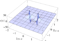
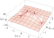
Fig. 1: Surfaces $\epsilon(\mathop{\rm Re}u,\mathop{\rm Im}u)$ (left panel) and $\tilde{\epsilon}(\mathop{\rm Re}u,\mathop{\rm Im}u)$ (right panel) showing singularities at $u=\pm i/2$ and at $u=\pm i/2$, $u=\pm 3i/2$, respectively.

Dissipation assisted entropy reduction.— The fact that the effective quasiparticle dispersion $\tilde{\epsilon}(u)$ has an additional singularity at $u=\pm 3i/2$ compared to $\epsilon(u)$, see Fig. 1, leads, as described below, to a surprising sub-extensive scaling of von Neumann entropy of NESS as opposed to Gibbs states. The effect is most clearly illustrated and qualitatively explained in the quasi-particle sector $M=1$, containing $N$ Bethe eigenstates $\ket{\alpha}\equiv\psi(u_{\alpha})$ parameterized by the solutions $u_{\alpha}$, $\alpha=1,\ldots N$, of the BAEs (10). Among the $N$ single-particle solutions there are always $N-1$ real solutions, say $u_{2},\ldots,u_{N}$, and one boundary localized imaginary solution $u_{1}$, lying exponentially close to the extra singularity due to dissipative dressing, namely, $u_{1}=i(3/2+O(2^{-N}))$, see left panel of Fig. 2. Explicitly, from (10) we find $u_{1}-3i/2\equiv\delta=3i2^{-2N-1}(1+O(N\delta))$. The corresponding dressed energy $\tilde{\epsilon}(u_{1})$ is drastically renormalized by the singularity, acquiring a negative amplitude linearly growing with system size, $\tilde{\epsilon}(u_{1})\approx-2(N+1)\log 2+\log 9$ [13]. On the other hand, for real (plain wave type) solutions, the dressed and original energies are comparable. As a result, $e^{-\tilde{\epsilon}(u_{1})}\gg e^{-\tilde{\epsilon}(u_{\alpha})}$ for $\alpha>1$, and in the NESS, the boundary localized Bethe eigenstate $\psi(u_{1})$ comes with an exponentially large (in system size $N$) relative weight in the sum (5) with respect to the other $M=1$ eigenstates $\psi(u_{\alpha})$, see right panel of Fig. 2.

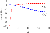
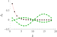
Fig. 2: Left panel: quasiparticle energies $\epsilon(u_{\alpha})$ (blue joined points) and $\tilde{\epsilon}(u_{\alpha})$ (red joined points) in the $XXX$ model with $N=18$ spin, in the block with one magnon $M=1$. The state $\alpha=1$ is a localized Bethe state with $u_{1}\simeq 3i/2+ie^{-24.5}$, see [13] for analytics. Right panel: coefficients $A_{k}$ of the normalized localized Bethe state $\ket{\alpha=1}=\sum_{k=1}^{N}A_{k}\ \sigma_{k}^{-}\ket{{\rm vac}}$ (black points). The dashed red line is the fit $A_{k}=1.7\times 2^{-k}$. The green joined points are the coefficients $\mathop{\rm Re}A_{k}$ and $\mathop{\rm Im}A_{k}$ for the plain-wave like Bethe state with $u_{3}\simeq-2.6934$.

This mechanism predicting boundary-localized Bethe states to yield dominant contribution to NESS can be qualitatively extended to higher but fixed $M$. However, understanding physics at fixed magnetization density $M/N$ would require controlling thermodynamic Bethe ansatz in the presence of boundary fields and our dissipative dressing. We leave this for future research while here we only demonstrate the phenomenology with some numerics. In Fig. 3 we show the scaling of von Neumann entropy $S(\rho)=-\operatorname{tr}\!{\rho}\log\rho$ on system size $N$ for both $\rho=\rho_{\rm NESS}$ and $\rho=\rho_{\rm Gibbs}$. We observe a clear sub-extensive scaling $S(\rho_{\rm NESS})/N\simeq 1/N^{0.7}$ for NESS, while in the Gibbs state we have an extensive entropy $S(\rho_{\rm Gibbs})/N\simeq{\rm const}$. This result is compared to the case where we add an integrabilty breaking term to $H_{D}$ (staggered magnetic field), case in which both entropies (Gibbs and NESS) scale extensively with $N$.

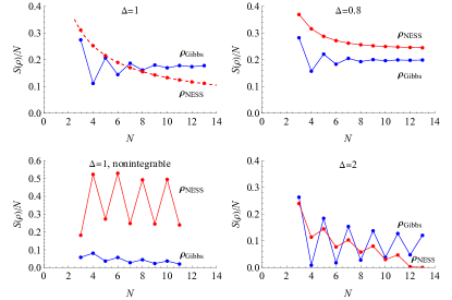
Fig. 3: Von Neumann entropy $S(\rho)=-\operatorname{tr}\!{(\rho\log\rho)}$ per spin versus the system size $N$ for $\rho=\rho_{\mathrm{Gibbs}}$ (blue points) and $\rho=\rho_{\rm NESS}$ (red points), illustrating the dissipation assisted entropy reduction. Left upper panel corresponds to the isotropic Heisenberg model $\Delta=1$, red dashed line is a fit given by $2/(3N^{0.7})$. Left bottom panel shows a nonintegrable case in which a staggered magnetic field $(-1)^{j}h\sigma^{z}_{j}$, with $h=1.5$, has been added. Right panels correspond to the anisotropic Heisenberg model in the easy plane $\Delta<1$ and easy axis $\Delta>1$ regime.

In Fig. 4 we compare the distribution of eigenvalues of $H_{D}$, energies $E_{\alpha}$, with that of the eigenvalues of $-\log\rho_{\rm NESS}$, energies $\tilde{E}_{\alpha}$, for the same integrable and non-integrable cases of Fig. 3.

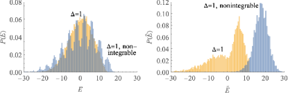
Fig. 4: Distribution of the eigenvalues $E$ of $-\log\rho_{\mathrm{Gibbs}}$ (left panel) and $\tilde{E}$ of $-\log\rho_{\mathrm{NESS}}$ (right panel) for the $XXX$ model with $N=13$. In both panels, the yellow and blue histograms correspond, respectively, to the integrable and nonintegrable cases of Fig. 3 with $\Delta=1$. The asymmetricity of $P(\tilde{E})$ for the integrable case is due to the dissipative dressing of quasiparticle energies (12) and it leads to subextensive entropy growth, see Fig. 3.

Dissipative dressing of quasiparticles in other integrable systems.— We now show that the dissipative dressing effect (2) is not restricted to the isotropic $XXX$ model but is a rather generic phenomenon, present in other integrable spin chains with anisotropic Heisenberg exchange interaction, with or without $U(1)$ symmetry.

Our first example is the $XXZ$ model with Hamiltonian

$$H_{XXZ}=\sum_{n=1}^{N-1}\vec{\sigma}_{n}\cdot\hat{J}\vec{\sigma}_{n+1}+h_{1}+h_{N},$$ (13)

where $\hat{J}=\mathrm{diag}(1,1,\Delta)$, $h_{1}=-\sigma_{1}^{z}\Delta$ and $h_{N}=\sigma_{N}^{z}\Delta$. This model was treated in its more general version (arbitrary longitudinal boundary fields) in the pioneering paper of Sklyanin [6]. The BAEs are as in (10) with the replacement $u^{[k]}=\sinh(u+ik\gamma/2)$, where $\cos\gamma=\Delta$. The spectrum of $H_{XXZ}$ is given by (8) with $E_{0}=(N-1)\Delta$ and quasiparticle energies

$$\epsilon(u)=\frac{-2\sin^{2}\gamma}{\sinh(u+\frac{i\gamma}{2})\sinh(u-\frac{i\gamma}{2})}.$$ (14)

Model (13) keeps $U(1)$ invariance and can be treated in the same way as its isotropic counterpart (3). The corresponding dissipative model is constructed by coupling an $XXZ$ chain with $N+2$ spins to fully polarizing dissipative baths at its edges and taking the quantum Zeno limit, see [13]. The rates of the associated auxiliary Markov process (6) have exactly the same expression (4), where $\ket{\alpha}$ are the eigenstates of (13).

Following the same steps as for the $XXX$ model and using the results [15], we obtain $\rho_{NESS}$ in the form (2) with the dressed dispersion relation

$$\tilde{\epsilon}(u) =\log\left|\frac{\sinh(u+\frac{3i\gamma}{2})\ \sinh(u-\frac{3i\gamma}{2})}{\sinh(u+\frac{i\gamma}{2})\ \sinh(u-\frac{i\gamma}{2})}\right|$$

$$=\log|1-\epsilon(u)\Delta|,\qquad\Delta=\cos\gamma,$$ (15)

containing an additional singularity as in (12). We find that one-magnon sector contains boundary localized states generated by Bethe roots exponentially close to the singularity , for $\Delta>1/2$ and for sufficiently large $N$ [13]. Like in the isotropic case, the weight of such states in the NESS will be drastically renormalized by the dressing. By setting $\gamma\rightarrow\delta$, $u\rightarrow\delta u$ and letting $\delta\rightarrow 0$ one recovers the isotropic result (12). Note that $\gamma$ real and $\gamma$ imaginary correspond to $XXZ$ models with easy plane $|\Delta|=|\cos\gamma|<1$ and easy axis anisotropy $|\Delta|>1$. For $|\Delta|<1$ we have a critical regime with algebraically decaying correlations, while for $|\Delta|>1$ a gapped regime, with correlations decaying exponentially with distance. The quasiparticle features, e.g., the spectrum, and hence the thermodynamic properties for the easy plane and easy axis regimes are completely different, we thus expect the two regimes to show qualitatively different dressing effects. Indeed, we observe a distinct behavior of the entropy of NESS, see right column of Fig. 3, showing fast, perhaps exponential decay of $S(\rho_{\rm NESS})/N$ in the gapped regime $|\Delta|>1$, and saturation $S(\rho_{\rm NESS})/N\sim{\rm const}$ in the critical regime $|\Delta|<1$.

Critical $XXZ$ model with chiral invariant subspace.—Our next example is a critical $XXZ$ model (13), with $\gamma$ real, but with non-diagonal boundary fields $h_{1},h_{N}$, which break the $U(1)$ symmetry

$$h_{1}=\sigma_{1}^{x},\qquad h_{N}=\sigma_{N}^{x}\cos\varphi(M)+\sigma_{N}^{y}\sin\varphi(M),$$ (16)

$$\varphi(M)=(N+1-2M)\gamma.$$ (17)

It was shown in [16, 17] that for integer $M$ values $M=0,1,\dots,N+1$ this model has a chiral invariant subspace $G_{M}$ spanned by pieces of spin helices of the same period and of the same helicity sign, of dimension $d_{M}=\binom{N+1}{M}$. The Gibbs state restricted to the invariant subspace $G_{M}$ has the form (1) with $\alpha=1,\dots,d_{M}$ and $j=1,\dots,M$. The Bethe rapidities, $u_{j\alpha}$, satisfy BAEs of the type (10), see [13], and $\epsilon(u)$ is given by the same expression (14) as for the conventional, magnetization carrying quasiparticles. In contrast to the previous “longitudinal case”, $E_{0}=(N+1)\Delta$ is not the energy of the vacuum state $\ket{\uparrow}^{\otimes N}$, but it represents the energy of the chiral vacuum, an exact spin helix with period $2\pi/\gamma$.

The corresponding dissipative model is obtained by coupling an $XXZ$ chain of $N+2$ spins with fields (16) to fully polarizing dissipative baths at its edges, projecting the respective spins on states polarized in the $xy$-plane with relative angle $\varphi(M)$. Operators $g_{L}$ and $g_{R}$ in (4) are given by $g_{L}=\Delta\sigma_{1}^{z}-\sigma_{1}^{+}+\sigma_{1}^{-}$ and $g_{R}=\Delta\sigma_{N}^{z}-e^{-i\varphi(M)}\sigma_{N}^{+}+e^{i\varphi(M)}\sigma_{N}^{-}$. The corresponding BAEs are as in [13]. We find that the NESS has exactly the same form (2) with $\alpha=1,\dots,d_{M}$ and $j=1,\dots,M$, but with dressed quasiparticle energies

$$\tilde{\epsilon}(u)=2\log\left|\frac{\cosh\left(u+\frac{i\gamma}{2}\right)\cosh\left(u-\frac{i\gamma}{2}\right)}{\sinh\left(u+\frac{i\gamma}{2}\right)\sinh\left(u-\frac{i\gamma}{2}\right)}\right|$$

$$=2\log\left|\epsilon(u)+2(\Delta-\Delta^{-1})\right|+2\log\left|\frac{\Delta}{2(1-\Delta^{2})}\right|.$$ (18)

We would like to stress that these quasiparticles do not carry fixed magnetization (as in the longitudinal $U(1)$ case), but rather form domain walls, or kinks, on top of a chiral “background”, see [18] for more details. As a result, the dressed energies (18) of chiral quasiparticles differ from that of conventional $XXZ$ magnetization-carrying quasiparticles (15) even though the bare dispersions (14) are the same.

$XYZ$ model with chiral invariant subspace.— Finally we consider the most general integrable spin chain with nearest neighbor interaction, the fully anisotropic $XYZ$ spin chain

$$H_{XYZ}=\sum_{n=1}^{N-1}\vec{\sigma}_{n}\hat{J}\vec{\sigma}_{n+1}+h_{1}(\vec{n}_{l})+h_{N}(\vec{n}_{r}),$$ (19)

with $\hat{J}=\mathrm{diag}(J_{x},J_{y},J_{z})$. The couplings $J_{\alpha}$ are conveniently parameterized in terms of elliptic theta-functions with anisotropy parameter $\eta$ and quasi-period $\tau=i$, $\theta_{\alpha}(\eta)\equiv\theta_{\alpha}(\eta,\tau=i)$,

$$\{J_{x},J_{y},J_{z}\}=\left\{\frac{\theta_{4}(\eta)}{\theta_{4}(0)},\frac{\theta_{3}(\eta)}{\theta_{3}(0)},\frac{\theta_{2}(\eta)}{\theta_{2}(0)}\right\}.$$ (20)

The boundary fields $h_{1},h_{N}$ have the form $h_{1}(\vec{n}_{l})=(\hat{J}\vec{n}_{l})\cdot\vec{\sigma_{1}}$ and $h_{N}(\vec{n}_{r})=(\hat{J}\vec{n}_{r})\cdot\vec{\sigma_{N}}$, where $\vec{n}_{l},\vec{n}_{r}$ are unit vectors. These vectors are parameterized by two complex parameters $u_{l},u_{r}$, satisfying $u_{r}=u_{l}+(N+1-2M)\eta$, which is an analog of Eq. (17). Further details are given in [13]. For integer $M$ the Hamiltonian (19) has an invariant subspace of dimension $d_{M}=\binom{N+1}{M}$ which allows to consider a Gibbs state restricted to this subspace.

The corresponding dissipative model is obtained by coupling an $XYZ$ chain with $N+2$ spins to fully polarizing dissipative baths at the edges, projecting the left/right spins on states polarized along $\vec{n}_{l}$/$\vec{n}_{r}$. Numerical investigations lead us to conjecture that the corresponding $\rho_{\rm NESS}$ restricted to the invariant subspace still has the form (2) with $\alpha=1,\dots,d_{M}$, $j=1,\dots,M$ and dressed quasiparticle energies

$$\begin{split}&\tilde{\epsilon}(u)=2\log\left|\frac{Q\left(\frac{1+\tau}{2}+i\mathop{\rm Im}u_{l},u\right)}{Q(0,u)}\right|,\\ &Q(x,u)=\theta_{1}\left(x-u+\tfrac{\eta}{2}\right)\theta_{1}\left(x+u+\tfrac{\eta}{2}\right),\end{split}$$ (21)

while the bare energies $\epsilon(u)$ are

$$\begin{split}&\epsilon(u)=2\left[g(u-\tfrac{\eta}{2})-g(u+\tfrac{\eta}{2})\right],\\ &g(u)=\frac{\bar{\theta}_{1}(\eta)\bar{\theta}_{1}^{\prime}(u)}{\bar{\theta}_{1}^{\prime}(0)\bar{\theta}_{1}(u)}.\end{split}$$ (22)

By letting $i\mathop{\rm Im}u_{l}=\tau/2$ and $\tau\rightarrow+i\infty$ one recovers the $XXZ$ limit (18).

Discussion.—We have developed an explicit Bethe ansatz procedure for diagonalizing the steady state density operators of boundary dissipatively driven integrable quantum spin chains in the limit of large dissipation, alias the Zeno regime. This becomes possible due to a suprising phenomenon of “dissipative dressing” of quasiparticle energies in integrable coherent systems exposed to a dissipation. We find a general mechanism of entropy reduction due to dissipation—pushing the steady state density matrix towards a pure state—which is a consequence of additional singularities arising in the quasiparticle dispersion relation due to dissipative dressing.

Our results should have applications in state engineering and dissipative state preparation. Moreover, we expect analogous emergent integrability of the steady state in the discrete-time case of an integrable Floquet $XXX$/$XXZ$/$XYZ$ circuit, where boundary dissipation can be conveniently implemented by the so-called reset channel [10].

Supplemental Material

This Supplemental Material contains six sections. In S-I we list quantum models under dissipation and the respective coherent models. In S-II we prove our main result, i.e. obtain the dissipatively-dressed energies for the U(1) XXZ Hamiltonian, while S-III and S-IV contain some further technical details. S-V and S-VI contain details for XXZ and XYZ model with chiral invariant subspaces.

Appendix A S-I. Zeno NESS: quantum models with dissipation, effectively governed by the Hamiltonians (3),(13), (16),(19), and (3) with staggering

For all the examples of the main text, i.e. coherent models with Hamiltonians $H_{D}$ (3,13,16,19) there exist a quantum spin chain with boundary dissipation, NESS of which shares the same set of eigenstates.

For $H_{D}$ from (3) this is an XXX model of $N+2$ sites $H=\sum_{n=0}^{N}\vec{\sigma}_{n}\vec{\sigma}_{n+1}$, in which the first spin at position $0$ and the last spin at position $N+1$ are projected, by coupling them to a dissipative bath, on pure states, spin down $\ket{\downarrow}\bra{\downarrow}$ and spin up $\ket{\uparrow}\bra{\uparrow}$, described by the Lindblad Master equation of the form

$$\frac{\partial\rho(\Gamma,t)}{\partial t}=-i[H,\rho]+\Gamma\left({\cal D}_{L_{1}}[\rho]+{\cal D}_{L_{2}}[\rho]\right)$$ (S-1)

$${\cal D}_{L}[\rho]=L\rho L^{\dagger}-\frac{1}{2}\left(L^{\dagger}L\rho+\rho L^{\dagger}L\right)$$

where $L_{1}$,$L_{2}$ are polarization targeting Lindblad operators

$$L_{1}=\sigma_{0}^{-},\quad L_{1}=\sigma_{N+1}^{+}$$ (S-2)

making the states of the respective qubits relax onto pure states $\ket{\downarrow}\bra{\downarrow}$ and $\ket{\uparrow}\bra{\uparrow}$. The typical relaxation time for sufficienlly large $\Gamma$ (in Zeno limit regime) scales as inverse dissipation strength $t_{\rm relaxation}\sim\Gamma^{-1}$.

The respective Zeno NESS is the stationary solution of (S-1) $\frac{\partial\rho}{\partial t}=0$ in the $\Gamma\rightarrow\infty$ limit, is unique and is given by

$$\ket{\psi_{0}}\bra{\psi_{0}}\otimes\rho_{\rm NESS}\otimes\ket{\psi_{N+1}}\bra{\psi_{N+1}}=\lim_{\Gamma\rightarrow\infty}\lim_{t\rightarrow\infty}\rho(\Gamma,t),$$ (S-3)

where $\ket{\psi_{0}}\bra{\psi_{0}}$ and $\ket{\psi_{N+1}}\bra{\psi_{N+1}}$ are targeted qubit states, $\ket{\downarrow}\bra{\downarrow}$ and $\ket{\uparrow}\bra{\uparrow}$ respectively.

The above Zeno NESS, after tracing out the dissipation -affected spins $k=0,N+1$, commutes with the “dissipation-projected” Hamiltonian $H_{D}$ from (3) as shown in [12],

$$[\rho_{\rm NESS},H_{D}]=0.$$ (S-4)

For other cases: U1 XXZ (13), chiral XXZ (16), chiral XYZ (19), the respective NESS and the equation of evolution is given by the same (S-3), (S-1), where the definitions of $H_{D}$ and $L_{1},L_{2}$ change accordingly. The operators $L_{1},L_{2}$ have form of polarization-targeting operators

$$L_{1}=\ket{\psi_{0}}\bra{\psi_{0}^{\perp}},\quad L_{2}=\ket{\psi_{N+1}}\bra{\psi_{N+1}^{\perp}},$$ (S-5)

and the corresponding Lindblad dissipators ${\cal D}_{L_{1}}$, ${\cal D}_{L_{2}}$ target pure qubit states $\ket{\psi_{0}}\bra{\psi_{0}}$, $\ket{\psi_{N+1}}\bra{\psi_{N+1}}$ at sites $0,N+1$ respectively.

For the cases: U1 XXZ (13), chiral XXZ (16), chiral XYZ (19), the targeted states explicitly read:

$$\ket{\psi_{0}}=\ket{\downarrow},\quad\ket{\psi_{N+1}}=\ket{\uparrow},\quad\mbox{ U(1) XXZ, XXX and XXX with staggered field}$$ (S-6)

$$\ket{\psi_{0}}=\frac{1}{\sqrt{2}}(\ket{\uparrow}+\ket{\downarrow}),\quad\ket{\psi_{N+1}}=\frac{1}{\sqrt{2}}(\ket{\uparrow}+e^{i\varphi(M)}\ket{\downarrow}),\quad\mbox{ chiral XXZ}$$ (S-7)

$$\ket{\psi_{0}}\bra{\psi_{0}}=\frac{I}{2}+\frac{1}{2}\sum_{\alpha=x,y,z}n_{l}^{\alpha}\sigma_{0}^{\alpha},\quad\ket{\psi_{N+1}}\bra{\psi_{N+1}}=\frac{I}{2}+\frac{1}{2}\sum_{\alpha=x,y,z}n_{r}^{\alpha}\sigma_{N+1}^{\alpha},\quad\mbox{ chiral XYZ}$$ (S-8)

For the non-integrable example, featured on Figs. 3,4, the coherent model ( $H_{D}$ ) has the form of an XXX model with staggered magnetic field,

$$H_{D}=\sum_{n=1}^{N-1}\vec{\sigma}_{n}\vec{\sigma}_{n+1}+h\sum_{n=1}^{N-1}(-1)^{n}\sigma_{n}^{z}-\sigma_{1}^{z}+\sigma_{N}^{z},\quad h=1.5,$$ (S-9)

while the dissipation-affected model is given by (S-3), (S-1), with $H=\sum_{n=0}^{N}\vec{\sigma}_{n}\vec{\sigma}_{n+1}+h\sum_{n=1}^{N-1}(-1)^{n}\sigma_{n}^{z}$ and the polarization targeting Lindblad operators (S-2).

For all listed models, the NESS (S-3) is unique and is given by $\sum_{\alpha}\nu_{\alpha}\ket{\alpha}\bra{\alpha}$ where $\ket{\alpha}$ are eigenstates of the respective $H_{D}$ and $\nu_{\alpha}=e^{-\tilde{E}_{\alpha}}$ are solutions of

$$\sum_{\beta\neq\alpha}w_{\beta\alpha}\nu_{\beta}-\nu_{\alpha}\sum_{\beta\neq\alpha}w_{\alpha\beta}=0,\quad\alpha=1,2,\dots$$ (S-10)

The rates of the auxiliary classical Markov process are given by

$$w_{\beta\alpha}=|\bra{\alpha}g_{L}\ket{\beta}|^{2}+|\bra{\alpha}g_{R}\ket{\beta}|^{2}.$$ (S-11)

see [12], where $g_{L},g_{R}$ are suitably chosen local operators, which depend on targeted states and the original Hamiltonian $H$. Explicitly, for pure targeted states with polarizations $\vec{n}_{L}\equiv\vec{n}(\theta_{L},\varphi_{L})=(\sin\theta_{L}\cos\varphi_{L},\sin\theta_{L}\sin\varphi_{L},\cos\theta_{L})$ and $\vec{n}_{R}=(\sin\theta_{R}\cos\varphi_{R},\sin\theta_{R}\sin\varphi_{R},\cos\theta_{R})$ and for a generic anisotropic Heisenberg Hamiltonian $H=\sum_{n=0}^{N}\vec{\sigma}_{n}\cdot(J\vec{\sigma}_{n+1})$ the operators $g_{L},g_{R}$ are given by

$$g_{L}=(J\vec{n_{L}}^{\prime})\cdot\vec{\sigma}_{1}-i(J\vec{n_{L}}^{\prime\prime})\cdot\vec{\sigma}_{1}$$ (S-12)

$$g_{R}=(J\vec{n_{R}}^{\prime})\cdot\vec{\sigma}_{N}-i(J\vec{n_{R}}^{\prime\prime})\cdot\vec{\sigma}_{N}$$ (S-13)

where $\vec{n}^{\prime}$ and $\vec{n}^{\prime\prime}$ are obtained from $\vec{n}\equiv\vec{n}(\theta,\varphi)$ as $\vec{n}^{\prime}=\vec{n}(\frac{\pi}{2}-\theta,\varphi+\pi)$ and $\vec{n}^{\prime\prime}=\vec{n}(\frac{\pi}{2},\varphi+\frac{\pi}{2})$. For specific models, $g_{L},g_{R}$ from (S-12), (S-13) reduce to those given in the main text.

The dissipatively dressed energies for $\nu_{\alpha}=e^{-\tilde{E}_{\alpha}}$ for the non-integrable model is obtained by solving (S-10) numerically.

For all examples with the dressed quasiparticle energies match the numerically obtained entries $\tilde{E}_{\alpha}$ (2).

Appendix B S-II. Derivation of Eqs. (12) and (15)

We first recall some details of well-known Bethe Ansatz solution of an open $XXZ$ model with diagonal boundary fields

$$H=\sum_{n=1}^{N-1}[\sigma_{n}^{x}\sigma_{n+1}^{x}+\sigma_{n}^{y}\sigma_{n+1}^{y}+\cosh\eta\,\sigma_{n}^{z}\sigma_{n+1}^{z}]+\frac{\sinh\eta}{\tanh p}\,\sigma_{1}^{z}+\frac{\sinh\eta}{\tanh q}\sigma_{N}^{z}.$$ (S-14)

Here, $\cosh\eta\equiv\cos\gamma$ is the anisotropic parameter.

The $R$-matrix and $K$-matrices for the model are

$$R(u) =\left(\begin{array}[]{cccc}\sinh(u+\eta)&0&0&0\\ 0&\sinh u&\sinh\eta&0\\ 0&\sinh\eta&\sinh u&0\\ 0&0&0&\sinh(u+\eta)\\ \end{array}\right),$$ (S-19)

$$K^{-}(u) =\left(\begin{array}[]{cc}\sinh(p+u-\frac{\eta}{2})&0\\ 0&\sinh(p-u+\frac{\eta}{2})\\ \end{array}\right),$$ (S-22)

$$K^{+}(u) =\left(\begin{array}[]{cc}\sinh(q+u+\frac{\eta}{2})&0\\ 0&\sinh(q-u-\frac{\eta}{2})\\ \end{array}\right).$$ (S-25)

Let us introduce the one-row monodromy matrices

$$\begin{aligned} T_{0}(u)&=R_{0,N}(u-\tfrac{\eta}{2})\ldots R_{0,1}(u-\tfrac{\eta}{2}),\\ \hat{T}_{0}(u)&=R_{1,0}(u-\tfrac{\eta}{2})\ldots R_{N,0}(u-\tfrac{\eta}{2}),\end{aligned}$$ (S-26)

and the double-row monodromy matrix

$$\mathcal{U}_{0}^{-}(u)=T_{0}(u)K_{0}^{-}(u)\hat{T}_{0}(u)=\left(\begin{array}[]{cc}A_{-}(u)&B_{-}(u)\\ C_{-}(u)&D_{-}(u)\\ \end{array}\right).$$ (S-29)

The transfer matrix is given by

$$t(u)={\rm tr}_{0}\{K_{0}^{+}(u)\mathcal{U}^{-}_{0}(u)\}.$$ (S-30)

The Hamiltonian (S-14) rewritten in terms of the transfer matrix reads

$$H=\sinh\eta\left.\frac{\partial\ln t(u)}{\partial u}\right|_{u=\frac{\eta}{2}}-N\cosh\eta-\tanh\eta\sinh\eta.$$ (S-31)

The eigenvalue of the quantum transfer matrix can be given by the following $T-Q$ relation

$$\Lambda(u)= \frac{\sinh(2u+\eta)}{\sinh(2u)}\prod_{s=p,q}\sinh(u+s-\tfrac{\eta}{2})\sinh^{2N}(u+\tfrac{\eta}{2})\prod_{j=1}^{m}\frac{\sinh(u-\lambda_{j}-\eta)\sinh(u+\lambda_{j}-\eta)}{\sinh(u-\lambda_{j})\sinh(u+\lambda_{j})}$$

$$+\frac{\sinh(2u-\eta)}{\sinh(2u)}\prod_{s=p,q}\sinh(u-s+\tfrac{\eta}{2})\sinh^{2N}(u-\tfrac{\eta}{2})\prod_{j=1}^{m}\frac{\sinh(u+\lambda_{j}+\eta)\sinh(u-\lambda_{j}+\eta)}{\sinh(u+\lambda_{j})\sinh(u-\lambda_{j})}.$$ (S-32)

The Bethe roots $\{\lambda_{1},\ldots,\lambda_{m}\}$ in (S-32) satisfy the following Bethe ansatz equations (BAEs)

$$\left[\frac{\sinh(\lambda_{j}+\frac{\eta}{2})}{\sinh(\lambda_{j}-\frac{\eta}{2})}\right]^{2N}\prod_{s=p,q}\frac{\sinh(\lambda_{j}+s-\frac{\eta}{2})}{\sinh(\lambda_{j}-s+\frac{\eta}{2})}\prod_{k\neq j}^{m}\frac{\sinh(\lambda_{j}-\lambda_{k}-\eta)\sinh(\lambda_{j}+\lambda_{k}-\eta)}{\sinh(\lambda_{j}+\lambda_{k}+\eta)\sinh(\lambda_{j}-\lambda_{k}+\eta)}=1,\qquad j=1,,\ldots,m.$$ (S-33)

Multiplying the left and right sides of BAEs for all $j$, we get

$$\prod_{j=1}^{m}\left[\frac{\sinh(\lambda_{j}+\frac{\eta}{2})}{\sinh(\lambda_{j}-\frac{\eta}{2})}\right]^{N}\frac{\sinh^{\frac{1}{2}}(\lambda_{j}+q-\tfrac{\eta}{2})\sinh^{\frac{1}{2}}(\lambda_{j}+p-\tfrac{\eta}{2})}{\sinh^{\frac{1}{2}}(\lambda_{j}-q+\tfrac{\eta}{2})\sinh^{\frac{1}{2}}(\lambda_{j}-p+\tfrac{\eta}{2})}=\pm\prod_{1\leq j<k\leq m}\frac{\sinh(\lambda_{j}+\lambda_{k}+\eta)}{\sinh(\lambda_{j}+\lambda_{k}-\eta)}.$$ (S-34)

The energy of the system in terms of the Bethe roots reads

$$E=\sum_{j=1}^{m}\frac{2\sinh^{2}\eta}{\sinh(\lambda_{j}+\frac{\eta}{2})\sinh(\lambda_{j}-\frac{\eta}{2})}+\sinh\eta(\coth p+\coth q)+(N-1)\cosh\eta.$$ (S-35)

B.1 Expressing local operators $\sigma_{1}^{\pm}$ and $\sigma_{N}^{\pm}$ in terms of monodromy matrix elements

The trigonometric $R$-matrix possesses the following properties:

$$\begin{aligned} &R_{1,2}(0)=\sinh\eta P_{1,2},\\ &R_{1,2}(u)R_{2,1}(-u)=\sinh(\eta+u)\sinh(\eta-u)\times\mathbb{I},\\ &R_{1,2}(u)=-\sigma_{1}^{y}R^{t_{1}}_{1,2}(-u-\eta)\sigma_{1}^{y}.\end{aligned}$$ (S-36)

It is easy to check that

$${\rm tr}_{0}\{\sigma_{0}^{-}K_{0}^{+}(u)\mathcal{U}_{0}^{-}(u)\}=\sinh(q+u+\tfrac{\eta}{2})B_{-}(u),$$ (S-37)

$${\rm tr}_{0}\{\sigma_{0}^{+}K_{0}^{+}(u)\mathcal{U}_{0}^{-}(u)\}=\sinh(q-u-\tfrac{\eta}{2})C_{-}(u).$$ (S-38)

We have

$${\rm tr}_{0}\{\sigma_{0}^{-}K_{0}^{+}(-\tfrac{\eta}{2})\mathcal{U}_{0}^{-}(-\tfrac{\eta}{2})\}$$

$$={\rm tr}_{0}\{[\sigma_{0}^{-}K_{0}^{+}(-\tfrac{\eta}{2})R_{0,N}(-\eta)\ldots R_{0,1}(-\eta)]^{t_{0}}[K_{0}^{-}(-\tfrac{\eta}{2})R_{1,0}(-\eta)\ldots R_{N,0}(-\eta)]^{t_{0}}\}$$

$$={\rm tr}_{0}\{[R_{0,N}(-\eta)\ldots R_{0,1}(-\eta)]^{t_{0}}[\sigma_{0}^{-}K_{0}^{+}(-\tfrac{\eta}{2})]^{t_{0}}[R_{1,0}(-\eta)\ldots R_{N,0}(-\eta)]^{t_{0}}[K_{0}^{-}(-\tfrac{\eta}{2})]^{t_{0}}\}$$

$$={\rm tr}_{0}\{R^{t_{0}}_{0,1}(-\eta)\ldots R^{t_{0}}_{0,N}(-\eta)[\sigma_{0}^{-}K_{0}^{+}(-\tfrac{\eta}{2})]^{t_{0}}R^{t_{0}}_{N,0}(-\eta)\ldots R^{t_{0}}_{1,0}(-\eta)[K_{0}^{-}(-\tfrac{\eta}{2})]^{t_{0}}\}$$

$$={\rm tr}_{0}\{R_{0,1}(0)\ldots R_{0,N}(0)[\sigma_{0}^{y}\sigma_{0}^{-}K_{0}^{+}(-\tfrac{\eta}{2})\sigma_{0}^{y}]^{t_{0}}R_{N,0}(0)\ldots R_{1,0}(0)[\sigma_{0}^{y}K_{0}^{-}(-\tfrac{\eta}{2})\sigma_{0}^{y}]^{t_{0}}\}$$

$$=\sinh^{2N}\!\!\eta[\sigma_{N}^{y}\sigma_{N}^{-}K_{N}^{+}(-\tfrac{\eta}{2})\sigma_{N}^{y}]^{t_{N}}{\rm tr}_{0}\{[\sigma_{0}^{y}K_{0}^{-}(-\tfrac{\eta}{2})\sigma_{0}^{y}]^{t_{0}}\}$$

$$=-2\cosh\eta\sinh p\sinh q\sinh^{2N}\!\!\eta\,\sigma_{N}^{-}.$$ (S-39)

Analogously, we get

$${\rm tr}_{0}\{\sigma_{0}^{+}K_{0}^{+}(-\tfrac{\eta}{2})\mathcal{U}_{0}^{-}(-\tfrac{\eta}{2})\}=-2\cosh\eta\sinh p\sinh q\sinh^{2N}\!\!\eta\,\sigma_{N}^{+}.$$ (S-40)

Then, we get the following relation between $\sigma_{N}^{\pm}$ and $B_{-}(-\tfrac{\eta}{2})$, $C_{-}(-\tfrac{\eta}{2})$

$$\sigma_{N}^{-}=-\frac{B_{-}(-\tfrac{\eta}{2})}{2\cosh\eta\sinh p\sinh^{2N}\!\!\eta},$$ (S-41)

$$\sigma_{N}^{+}=-\frac{C_{-}(-\tfrac{\eta}{2})}{2\cosh\eta\sinh p\sinh^{2N}\!\!\eta}.$$ (S-42)

One can rewrite the transfer matrix in another way

$$t(u) ={\rm tr}_{0}\{[K_{0}^{+}(u)T_{0}(u)]^{t_{0}}[K_{0}^{-}(u)\hat{T}_{0}(u)]^{t_{0}}\}$$

$$={\rm tr}_{0}\{T_{0}^{t_{0}}(u)[K_{0}^{+}(u)]^{t_{0}}\hat{T}_{0}^{t_{0}}(u)[K_{0}^{-}(u)]^{t_{0}}\}$$

$$={\rm tr}_{0}\{[K_{0}^{-}(u)]^{t_{0}}[\mathcal{U}^{+}_{0}(u)]^{t_{0}}\}$$

$$={\rm tr}_{0}\{K_{0}^{-}(u)\mathcal{U}^{+}_{0}(u)\},$$ (S-43)

where

$$[\mathcal{U}^{+}_{0}(u)]^{t_{0}} =T_{0}^{t_{0}}(u)[K_{0}^{+}(u)]^{t_{0}}\hat{T}_{0}^{t_{0}}(u)$$

$$=R_{0,1}^{t_{0}}(u-\tfrac{\eta}{2})\ldots R_{0,N}^{t_{0}}(u-\tfrac{\eta}{2})[K_{0}^{+}(u)]^{t_{0}}R_{N,0}^{t_{0}}(u-\tfrac{\eta}{2})\ldots R_{1,0}^{t_{0}}(u-\tfrac{\eta}{2})$$

$$=\left(\begin{array}[]{cc}A_{+}(u)&C_{+}(u)\\ B_{+}(u)&D_{+}(u)\\ \end{array}\right).$$ (S-46)

We obtain that

$$\sinh p\,B_{+}(\tfrac{\eta}{2}) ={\rm tr}_{0}\{\sigma_{0}^{-}K_{0}^{-}(\tfrac{\eta}{2})\mathcal{U}^{+}_{0}(\tfrac{\eta}{2})\}$$

$$={\rm tr}_{0}\{[\sigma_{0}^{-}K_{0}^{-}(\tfrac{\eta}{2})]^{t_{0}}[\mathcal{U}^{+}_{0}(\tfrac{\eta}{2})]^{t_{0}}\}$$

$$={\rm tr}_{0}\{[\sigma_{0}^{-}K_{0}^{-}(\tfrac{\eta}{2})]^{t_{0}}T_{0}^{t_{0}}(\tfrac{\eta}{2})[K_{0}^{+}(\tfrac{\eta}{2})]^{t_{0}}\hat{T}_{0}^{t_{0}}(\tfrac{\eta}{2})\}$$

$$={\rm tr}_{0}\{K_{0}^{+}(\tfrac{\eta}{2})T_{0}(\tfrac{\eta}{2})\sigma_{0}^{-}K_{0}^{-}(\tfrac{\eta}{2})\hat{T}_{0}(\tfrac{\eta}{2})\}$$

$$={\rm tr}_{0}\{K_{0}^{+}(\tfrac{\eta}{2})R_{0,N}(0)\ldots R_{1,0}(0)\sigma_{0}^{-}K_{0}^{-}(\tfrac{\eta}{2})R_{1,0}(0)\ldots R_{N,0}(0)\}$$

$$=\sinh^{2N}\!\!\eta\,\sigma_{1}^{-}K_{1}^{-}(\tfrac{\eta}{2}){\rm tr}_{0}\{K_{0}^{+}(\tfrac{\eta}{2})\}$$

$$=2\cosh\eta\sinh q\sinh p\sinh^{2N}\!\!\eta\,\sigma_{1}^{-},$$ (S-47)

$$\sinh p\,C_{+}(\tfrac{\eta}{2}) =2\cosh\eta\sinh q\sinh p\sinh^{2N}\!\!\eta\,\sigma_{1}^{+}.$$ (S-48)

Therefore, we need to calculate the quantity

$$\frac{|\bra{\mathbf{u}}\sigma_{1}^{-}\ket{\mathbf{v}}|^{2}+\bra{\mathbf{u}}\sigma_{N}^{+}\ket{\mathbf{v}}|^{2}}{|\bra{\mathbf{v}}\sigma_{1}^{-}\ket{\mathbf{u}}|^{2}+\bra{\mathbf{v}}\sigma_{N}^{+}\ket{\mathbf{u}}|^{2}} =\frac{|\bra{\mathbf{u}}\sigma_{1}^{-}\ket{\mathbf{v}}|^{2}}{|\bra{\mathbf{u}}\sigma_{N}^{-}\ket{\mathbf{v}}|^{2}}$$

$$=\left|\frac{\sinh p}{\sinh q}\right|^{2}\frac{|\bra{\mathbf{u}}B_{+}(\frac{\eta}{2})\ket{\mathbf{v}}|^{2}}{|\bra{\mathbf{u}}B_{-}(-\frac{\eta}{2})\ket{\mathbf{v}}|^{2}},$$ (S-49)

where

$$\mathbf{u}=\{u_{1},\ldots,u_{n+1}\},\qquad\mathbf{v}=\{v_{1},\ldots,v_{n}\}$$

are the solution of the BAEs (S-33).

B.2 Calculating the expression (S-49)

In the following we will recall some result of Ref. [15] to derive the ratio

$$\frac{\bra{\mathbf{u}}B_{+}(\frac{\eta}{2})\ket{\mathbf{v}}}{\bra{\mathbf{u}}B_{-}(-\frac{\eta}{2})\ket{\mathbf{v}}}.$$ (S-50)

appearing in (S-49). The Bethe state $\ket{\bf u}$ can be constructed by either $\prod_{j=1}^{n+1}B_{-}(u_{j})\ket{{\rm vac}}$ or $\prod_{j=1}^{n+1}B_{+}(u_{j})\ket{{\rm vac}}$ Inserting the expression of $\ket{\mathbf{v}}$, $\ket{\mathbf{u}}$ into (S-50), we get

$$\frac{\bra{\mathbf{u}}B_{+}(\frac{\eta}{2})\ket{\mathbf{v}}}{\bra{\mathbf{u}}B_{-}(-\frac{\eta}{2})\ket{\mathbf{v}}} =\frac{\bra{{\rm vac}}C_{-}(u_{1})\cdots C_{-}(u_{n+1})B_{+}(\tfrac{\eta}{2})B_{+}(v_{1})\ldots B_{+}(v_{n})\ket{{\rm vac}}}{\bra{{\rm vac}}C_{+}(u_{1})\cdots C_{+}(u_{n+1})B_{-}(-\tfrac{\eta}{2})B_{-}(v_{1})\ldots B_{-}(v_{n})\ket{{\rm vac}}}$$

$$\qquad\times\frac{\bra{{\rm vac}}C_{+}(u_{1})\cdots C_{+}(u_{n+1})B_{-}(v_{1})\ldots B_{-}(v_{n})\ket{{\rm vac}}}{\bra{{\rm vac}}C_{-}(u_{1})\cdots C_{-}(u_{n+1})B_{+}(v_{1})\ldots B_{+}(v_{n})\ket{{\rm vac}}}.$$ (S-51)

From Ref. [15], we know that

$$\frac{\bra{{\rm vac}}C_{-}(u_{1})\cdots C_{-}(u_{n+1})B_{+}(v_{1})\ldots B_{+}(v_{n})\ket{{\rm vac}}}{\bra{{\rm vac}}C_{+}(u_{1})\cdots C_{+}(u_{n+1})B_{-}(v_{1})\ldots B_{-}(v_{n})\ket{{\rm vac}}}=\prod_{j=1}^{n+1}\frac{\sinh(\eta-2u_{j})}{\sinh(\eta+2u_{j})}\prod_{j=1}^{n}\frac{\sinh(\eta+2v_{j})}{\sinh(\eta-2v_{j})}G(\{\mathbf{v}\};q,p)G(\{\mathbf{u}\};p,q),$$ (S-52)

where

$$G(\{\lambda_{1},\ldots,\lambda_{m}\};x,y)=\prod_{j=1}^{m}\frac{\sinh^{N}(\lambda_{j}-\frac{\eta}{2})}{\sinh^{N}(\lambda_{j}+\frac{\eta}{2})}\frac{\sinh(\lambda_{j}-x+\frac{\eta}{2})}{\sinh(\lambda_{j}+y-\frac{\eta}{2})}\prod_{1\leq r<s\leq m}\frac{\sinh(\lambda_{r}+\lambda_{s}+\eta)}{\sinh(\lambda_{r}+\lambda_{s}-\eta)}.$$ (S-53)

With the help of Theorem 4.1 and Corollary 4.1 in [15], we get

$$\frac{\bra{{\rm vac}}C_{-}(u_{1})\cdots C_{-}(u_{n+1})B_{+}(\tfrac{\eta}{2})B_{+}(v_{1})\ldots B_{+}(v_{n})\ket{{\rm vac}}}{\bra{{\rm vac}}C_{+}(u_{1})\cdots C_{+}(u_{n+1})B_{-}(-\tfrac{\eta}{2})B_{-}(v_{1})\ldots B_{-}(v_{n})\ket{{\rm vac}}} =\frac{\bra{{\rm vac}}C_{-}(u_{1})\cdots C_{-}(u_{n+1})B_{+}(\tfrac{\eta}{2})B_{+}(v_{1})\ldots B_{+}(v_{n})\ket{{\rm vac}}}{\bra{{\rm vac}}C_{+}(\frac{\eta}{2})C_{+}(-v_{1})\cdots C_{+}(-v_{n})B_{-}(-u_{1})\ldots B_{-}(-u_{n+1})\ket{{\rm vac}}}$$

$$=\frac{\mathcal{S}_{n+1}^{-,+}(\{\mathbf{u}\};\{\tfrac{\eta}{2},\mathbf{v}\})}{\mathcal{S}_{n+1}^{+,-}(\{-\mathbf{u}\};\{\tfrac{\eta}{2},-\mathbf{v}\})},$$ (S-54)

where

$$\mathcal{S}_{m}^{-,+}(\{\lambda\};\{\mu\})=\prod_{j=1}^{m}\sinh^{N}(\lambda_{j}-\tfrac{\eta}{2})\sinh^{N}(\lambda_{j}+\tfrac{\eta}{2})\,\frac{\det\,\mathcal{J}(\{\lambda\};\{\mu\})}{\det\,\mathcal{V}(\{\lambda\};\{\mu\})},$$ (S-55)

$$\mathcal{S}_{m}^{+,-}(\{\mu\};\{\lambda\})=\prod_{j=1}^{m}\sinh^{N}(\lambda_{j}+\tfrac{\eta}{2})\sinh^{N}(\lambda_{j}-\tfrac{\eta}{2})\,\frac{\det\,\mathcal{J}(\{\lambda\};\{\mu\})}{\det\,\mathcal{V}(\{\lambda\};\{\mu\})},$$ (S-56)

$$\mathcal{V}_{j,k}(\{\lambda\};\{\mu\})=\frac{\sinh(2\lambda_{j})\sinh(2\mu_{k}-\eta)}{\sinh(2\lambda_{j}-\eta)\sinh(\mu_{k}-\lambda_{j})\sinh(\mu_{k}+\lambda_{j})},$$ (S-57)

$$\mathcal{J}_{j,k}(\{\lambda\};\{\mu\})=\frac{\partial}{\partial\lambda_{j}}\Lambda(\mu_{k},\{\lambda\}).$$ (S-58)

The identity

$$\Lambda(u,\{\lambda\})=\Lambda(u,\{-\lambda\})=\Lambda(-u,\{-\lambda\}),$$ (S-59)

implies that

$$\frac{\det\,\mathcal{J}(\{\mathbf{u}\};\{\tfrac{\eta}{2},\mathbf{v}\})}{\det\,\mathcal{J}(\{-\mathbf{u}\};\{\tfrac{\eta}{2},-\mathbf{v}\})}=(-1)^{n+1}.$$ (S-60)

For the matrix $\mathcal{V}$, we have

$$\frac{\mathcal{V}_{j,1}(\{\mathbf{u}\};\{x,\mathbf{v}\})}{\mathcal{V}_{j,1}(\{-\mathbf{u}\};\{x,-\mathbf{v}\})}=\frac{\sinh(2u_{j}+\eta)}{\sinh(2u_{j}-\eta)},$$ (S-61)

$$\frac{\mathcal{V}_{j,k\neq 1}(\{\mathbf{u}\};\{x,\mathbf{v}\})}{\mathcal{V}_{j,k\neq 1}(\{-\mathbf{u}\};\{x,-\mathbf{v}\})}=-\frac{\sinh(2v_{k-1}-\eta)}{\sinh(2u_{j}-\eta)}\frac{\sinh(2u_{j}+\eta)}{\sinh(2v_{k-1}+\eta)}.$$ (S-62)

As a consequence, it can be verified that

$$\frac{\det\,\mathcal{V}(\{\mathbf{u}\};\{\tfrac{\eta}{2},\mathbf{v}\})}{\det\,\mathcal{V}(\{-\mathbf{u}\};\{\tfrac{\eta}{2},-\mathbf{v}\})}=(-1)^{n}\prod_{j=1}^{n+1}\frac{\sinh(2u_{j}+\eta)}{\sinh(2u_{j}-\eta)}\prod_{k=1}^{n}\frac{\sinh(2v_{k}-\eta)}{\sinh(2v_{k}+\eta)}.$$ (S-63)

Then, one can derive the following equation

$$\frac{\mathcal{S}_{n+1}^{-,+}(\{\mathbf{u}\};\{\tfrac{\eta}{2},\mathbf{v}\})}{\mathcal{S}_{n+1}^{+,-}(\{-\mathbf{u}\};\{\tfrac{\eta}{2},-\mathbf{v}\})}=-\prod_{j=1}^{n+1}\frac{\sinh(2u_{j}-\eta)}{\sinh(2u_{j}+\eta)}\prod_{k=1}^{n}\frac{\sinh(2v_{k}+\eta)}{\sinh(2v_{k}-\eta)}.$$ (S-64)

Substituting (S-52) and (S-64) into (S-51), we finally obtain

$$\frac{\bra{\mathbf{u}}B_{+}(\frac{\eta}{2})\ket{\mathbf{v}}}{\bra{\mathbf{u}}B_{-}(-\frac{\eta}{2})\ket{\mathbf{v}}} =G^{-1}(\{\mathbf{v}\};q,p)G^{-1}(\{\mathbf{u}\};p,q)$$

$$=\prod_{j=1}^{n+1}\frac{\sinh^{N}(u_{j}+\frac{\eta}{2})}{\sinh^{N}(u_{j}-\frac{\eta}{2})}\prod_{j=1}^{n+1}\frac{\sinh(u_{j}+q-\frac{\eta}{2})}{\sinh(u_{j}-p+\frac{\eta}{2})}\prod_{1\leq r<s\leq m}\frac{\sinh(u_{r}+u_{s}-\eta)}{\sinh(u_{r}+u_{s}+\eta)}$$

$$\qquad\times\prod_{k=1}^{n}\frac{\sinh^{N}(v_{k}+\frac{\eta}{2})}{\sinh^{N}(v_{k}-\frac{\eta}{2})}\frac{\sinh(v_{k}+p-\frac{\eta}{2})}{\sinh(v_{k}-q+\frac{\eta}{2})}\prod_{1\leq r<s\leq n}\frac{\sinh(v_{r}+v_{s}-\eta)}{\sinh(v_{r}+v_{s}+\eta)}$$

$$=\pm\prod_{j=1}^{n+1}\frac{\sinh^{\frac{1}{2}}(u_{j}+q-\frac{\eta}{2})}{\sinh^{\frac{1}{2}}(u_{j}-p+\frac{\eta}{2})}\frac{\sinh^{\frac{1}{2}}(u_{j}-q+\tfrac{\eta}{2})}{\sinh^{\frac{1}{2}}(u_{j}+p-\tfrac{\eta}{2})}\prod_{k=1}^{n}\frac{\sinh^{\frac{1}{2}}(v_{k}+p-\frac{\eta}{2})}{\sinh^{\frac{1}{2}}(v_{k}-q+\frac{\eta}{2})}\frac{\sinh^{\frac{1}{2}}(v_{k}-p+\tfrac{\eta}{2})}{\sinh^{\frac{1}{2}}(v_{k}+q-\tfrac{\eta}{2})}.$$ (S-65)

When $q=-p=\eta$, the BAEs are

$$\left[\frac{\sinh(\lambda_{j}+\frac{\eta}{2})}{\sinh(\lambda_{j}-\frac{\eta}{2})}\right]^{2N+1}\frac{\sinh(\lambda_{j}-\tfrac{3\eta}{2})}{\sinh(\lambda_{j}+\tfrac{3\eta}{2})}\prod_{k\neq j}^{m}\frac{\sinh(\lambda_{j}-\lambda_{k}-\eta)\sinh(\lambda_{j}+\lambda_{k}-\eta)}{\sinh(\lambda_{j}+\lambda_{k}+\eta)\sinh(\lambda_{j}-\lambda_{k}+\eta)}=1,\qquad j=1,\ldots,m,$$ (S-66)

$${\rm or}\, \left[\frac{\sinh(\lambda_{j}+\frac{i\gamma}{2})}{\sinh(\lambda_{j}-\frac{i\gamma}{2})}\right]^{2N+1}\frac{\sinh(\lambda_{j}-\tfrac{3i\gamma}{2})}{\sinh(\lambda_{j}+\tfrac{3i\gamma}{2})}\prod_{k\neq j}^{m}\frac{\sinh(\lambda_{j}-\lambda_{k}-i\gamma)\sinh(\lambda_{j}+\lambda_{k}-i\gamma)}{\sinh(\lambda_{j}+\lambda_{k}+i\gamma)\sinh(\lambda_{j}-\lambda_{k}+i\gamma)}=1,\qquad j=1,\ldots,m.$$ (S-67)

Then,

$$\frac{|\bra{\mathbf{u}}\sigma_{1}^{-}\ket{\mathbf{v}}|^{2}+\bra{\mathbf{u}}\sigma_{N}^{+}\ket{\mathbf{v}}|^{2}}{|\bra{\mathbf{v}}\sigma_{1}^{-}\ket{\mathbf{u}}|^{2}+\bra{\mathbf{v}}\sigma_{N}^{+}\ket{\mathbf{u}}|^{2}}$$

$$=\left|\prod_{j=1}^{n+1}\frac{\sinh(u_{j}+\frac{\eta}{2})}{\sinh(u_{j}+\frac{3\eta}{2})}\frac{\sinh(u_{j}-\tfrac{\eta}{2})}{\sinh(u_{j}-\tfrac{3\eta}{2})}\prod_{k=1}^{n}\frac{\sinh(v_{k}-\frac{3\eta}{2})}{\sinh(v_{k}-\frac{\eta}{2})}\frac{\sinh(v_{k}+\tfrac{3\eta}{2})}{\sinh(v_{k}+\tfrac{\eta}{2})}\right|$$

$$=\left|\prod_{j=1}^{n+1}\frac{\sinh(u_{j}+\frac{i\gamma}{2})}{\sinh(u_{j}+\frac{3i\gamma}{2})}\frac{\sinh(u_{j}-\tfrac{i\gamma}{2})}{\sinh(u_{j}-\tfrac{3i\gamma}{2})}\prod_{k=1}^{n}\frac{\sinh(v_{k}-\frac{3i\gamma}{2})}{\sinh(v_{k}-\frac{i\gamma}{2})}\frac{\sinh(v_{k}+\tfrac{3i\gamma}{2})}{\sinh(v_{k}+\tfrac{i\gamma}{2})}\right|,$$ (S-68)

which leads to Eq. (15).

Define

$$e^{ip_{j}}=\frac{\sinh(\lambda_{j}+\frac{\eta}{2})}{\sinh(\lambda_{j}-\frac{\eta}{2})}=\frac{\sinh(\lambda_{j}+\frac{i\gamma}{2})}{\sinh(\lambda_{j}-\frac{i\gamma}{2})}.$$ (S-69)

Then, the BAEs (S-66) can be rewritten as

$$e^{i(2N+1)p_{j}}\,\frac{e^{ip_{j}}-2\Delta}{1-2\Delta e^{ip_{j}}}\,\prod_{k\neq j}^{m}\prod_{\sigma=\pm 1}\frac{1-2\Delta e^{i\sigma p_{k}}+e^{ip_{j}+i\sigma p_{k}}}{1-2\Delta e^{ip_{j}}+e^{ip_{j}+i\sigma p_{k}}}=1,\qquad j=1,\ldots,m.$$ (S-70)

Remark.

In the case $\Delta>\frac{1}{2}$, when $N$ is large enough, the BAEs in (S-70) possess a solution in which one of the Bethe roots tends to $-i\log\frac{1}{2\Delta}$. It is noteworthy that as the parameter $\Delta$ approaches $\frac{1}{2}$, such solutions are observable only in very large scale systems. That is the reason why we can not see the phase transition at the point $\Delta=\frac{1}{2}$.

Substituting $\gamma\rightarrow\delta$, $u\rightarrow\delta u^{\prime}$ and letting $\delta\rightarrow 0$, one recovers the $XXX$ limit in Eq. (12).

Appendix C S-III. Boundary-localized eigenstates for XXZ model (13) in one-magnon sector $M=1$

We shall use the coordinate Bethe ansatz to construct the Bethe state with one magnon. For $M=1$ case, the Bethe state can be written as

$$\sum_{n=1}^{N}\mathcal{A}_{n}(p)\,\sigma_{n}^{-}\ket{\rm vac},\quad\mathcal{A}_{n}(p)=(e^{ip}-2\Delta)e^{inp}-\left(1-2\Delta e^{ip}\right)e^{i(1-n)p},$$ (S-71)

where $p$ satisfies the equation

$$e^{i(2N+1)p}(e^{ip}-2\Delta)-(1-2\Delta e^{ip})=0.$$ (S-72)

Most solutions of (S-72) are real. In some cases, Eq. (S-72) has an imaginary solution. Indeed, let us define the following function

$$\mathcal{W}(x)=x^{(2N+1)}(x-2\Delta)-(1-2\Delta x).$$ (S-73)

One can easily check that

$$\mathcal{W}(1)=0,\quad\mathcal{W}(\tfrac{1}{2\Delta})=(1-4\Delta^{2})(2\Delta)^{-2N-2},$$

$$\mathcal{W}(2\Delta)=4\Delta^{2}-1,\quad\mathcal{W}^{\prime}(1)=2+2N(1-2\Delta).$$ (S-74)

When

$$\Delta>\frac{1}{2},\quad N>\frac{1}{2\Delta-1},$$ (S-75)

we know

$$\mathcal{W}(\tfrac{1}{2\Delta})<0,\quad\mathcal{W}(1)=0,\quad\mathcal{W}^{\prime}(1)<0.$$ (S-76)

Therefore, $\mathcal{W}(x)$ has a zero in the interval $(\frac{1}{2\Delta},1)$ under the condition (S-75), and it will approaches $\frac{1}{2\Delta}$ as $N$ increases.

It also implies that Eq. (S-72) has an imaginary solution when $(\ref{imag;eq})$ is satisfied. When $N$ is large enough, this imaginary $p$ will gives a localized state with

$$\mathcal{A}_{n}(p)\approx\left(\frac{1}{2\Delta}-2\Delta\right)\left(\frac{1}{2\Delta}\right)^{n}.$$ (S-77)

The dressed energy in terms of $p$ is

$$\log|e^{-ip}(e^{ip}-2\Delta)(1-2\Delta e^{ip})|\overset{(\ref{BAE;M1})}{=}\log|e^{2iNp}(e^{ip}-2\Delta)^{2}|.$$ (S-78)

For the imaginary solution $e^{ip}\approx\frac{1}{2\Delta}$ ($N$ is large), the dressed energy approximate

$$\log|(2\Delta)^{-2N-2}(1-4\Delta^{2})^{2}|=-2(N+1)\log(2\Delta)+2\log(4\Delta^{2}-1).$$ (S-79)

In particular, for $\Delta=1$ we obtain

$$\tilde{\epsilon}=-2(N+1)\log 2+\log 9,$$ (S-80)

reported in the main text.

Appendix D S-IV. Kolmogorov relation of $w_{\alpha,\beta}$ for the diagonal boundary case

With the help of (S-68), we can derive that

$$w_{\alpha\beta}=\mathcal{F}_{\alpha}/\mathcal{F}_{\beta},$$ (S-81)

where $\mathcal{F}_{\alpha}$ depends only on the distribution of Bethe roots in $\ket{\alpha}$. Therefore, we conclude that the Kolmogorov relation holds for $w_{\alpha\beta}$

$$w_{\alpha\beta_{1}}w_{\beta_{1}\gamma}w_{\gamma\beta_{2}}w_{\beta_{2}\alpha}=w_{\alpha\beta_{2}}w_{\beta_{2}\gamma}w_{\gamma\beta_{1}}w_{\beta_{1}\alpha}.$$ (S-82)

Due to the Kolmogorov relation in (S-82), Eq. (7) is satisfied automatically.

Appendix E S-V. Derivation of Eq. (18)

First we recall some well-known details of Bethe ansatz solution of the $XXZ$ model with non-diagonal boundary field,

$$H_{D}=\sum_{n=1}^{N-1}[\sigma_{n}^{x}\sigma_{n+1}^{x}+\sigma_{n}^{y}\sigma_{n+1}^{y}+\Delta\,\sigma_{n}^{z}\sigma_{n+1}^{z}]+h_{1}+h_{N},\qquad\Delta=\cos\gamma,\qquad|\Delta|<1,$$

$$h_{1}=\sigma_{1}^{x},\qquad h_{N}=\sigma_{N}^{x}\cos\varphi(M)+\sigma_{N}^{y}\sin\varphi(M),\qquad\varphi(M)=(N+1-2M)\gamma,$$ (S-83)

where $M=0,\ldots,N-1$.

The exact solution of this model is given by the following Bethe ansatz equations [19, 18]

$$\left[\frac{\sinh(\lambda_{j}+\frac{i\gamma}{2})}{\sinh(\lambda_{j}-\frac{i\gamma}{2})}\right]^{2N+2}\left[\frac{\cosh(\lambda_{j}-\frac{i\gamma}{2})}{\cosh(\lambda_{j}+\frac{i\gamma}{2})}\right]^{2}\prod_{k\neq j}^{M}\frac{\sinh(\lambda_{j}+\lambda_{k}-i\gamma)\sinh(\lambda_{j}-\lambda_{k}-i\gamma)}{\sinh(\lambda_{j}+\lambda_{k}+i\gamma)\sinh(\lambda_{j}-\lambda_{k}+i\gamma)}=1,\qquad j=1,\ldots,M,$$ (S-84)

$$\mbox{or}\qquad e^{2i(N+1)p_{j}}\left[\frac{\Delta-e^{ip_{j}}}{1-\Delta e^{ip_{j}}}\right]^{2}=\prod_{\sigma=\pm}\prod_{k\neq j}^{M}\frac{1-2\Delta e^{ip_{j}}+e^{ip_{j}}e^{i\sigma p_{k}}}{1-2\Delta e^{i\sigma p_{k}}+e^{ip_{j}}e^{i\sigma p_{k}}},\qquad j=1,\ldots,M.$$ (S-85)

The energy in terms of Bethe roots is given by

$$E =-\sum_{j=1}^{M}\frac{2\sin^{2}\gamma}{\sinh(\lambda_{j}+\frac{i\gamma}{2})\sinh(\lambda_{j}-\frac{i\gamma}{2})}+(N+1)\Delta$$

$$=4\sum_{k=1}^{M}[\cos(p_{k})-\Delta]\textbf{}+(N+1)\Delta.$$ (S-86)

Let us introduce the following chiral basis states

$$\begin{split}&\bra{\Phi(n_{1},\ldots,n_{M})}=\exp\left[i\gamma\sum_{k}n_{k}\right]\bigotimes_{l_{1}=1}^{n_{1}}\phi(l_{1})\bigotimes_{l_{2}=n_{1}+1}^{n_{2}}\phi(l_{2}-2)\cdots\bigotimes_{l_{M+1}=n_{M}+1}^{N}\phi(l_{M+1}-2M),\\ &\phi(x)=\frac{1}{\sqrt{2}}(1,\,e^{-ix\gamma}).\end{split}$$ (S-87)

Then, the set

$$\bra{\Phi(n_{1},\ldots,n_{M})},\qquad 0\leq n_{1}<n_{2}\cdots<n_{M}\leq N$$

forms an invariant subspace of the Hamiltonian (S-83). One can use the chiral basis to expand the Bethe state and the corresponding expansion coefficients depend on the Bethe roots $\{p_{1},\ldots,p_{M}\}$ which are solutions of (S-85) [16, 18].

The Hamiltonian (S-83) can be associated to a quantum chain with dissipation as explained in section S-I. The respective reduced density matrix evolves with time towards a unique NESS $\sum_{\alpha}\nu_{\alpha}\ket{\alpha}\bra{\alpha}$ (commuting with (S-83) ), spectrum of which $\nu_{\alpha}=\exp(-\tilde{E}_{\alpha})$ consists of dissipatively dressed quasiparticles, and is given by the following proposition:

Hypothesis 1.

The NESS spectrum $\{\nu_{\alpha}\}$ is given by

$$\frac{\nu_{\beta}}{\nu_{\alpha}} =\prod_{j=1}^{M}\left|\frac{\cosh(\lambda_{j}^{(\alpha)}+\frac{\eta}{2})\cosh(\lambda_{j}^{(\alpha)}-\frac{\eta}{2})}{\sinh(\lambda_{j}^{(\alpha)}+\frac{\eta}{2})\sinh(\lambda_{j}^{(\alpha)}-\frac{\eta}{2})}\frac{\sinh(\lambda_{j}^{(\beta)}+\frac{\eta}{2})\sinh(\lambda_{j}^{(\beta)}-\frac{\eta}{2})}{\cosh(\lambda_{j}^{(\beta)}+\frac{\eta}{2})\cosh(\lambda_{j}^{(\beta)}-\frac{\eta}{2})}\right|^{2}$$

$$=\prod_{j=1}^{M}\left|\frac{\Delta+\Delta^{-1}-2\cos(p_{j}^{(\alpha)})}{\Delta+\Delta^{-1}-2\cos(p_{j}^{(\beta)})}\right|^{2},$$ (S-88)

where $\{\lambda_{j}^{(\alpha)}\}$ or $\{p_{j}^{(\alpha)}\}$ are the Bethe roots corresponding to $\ket{\alpha}$.

Remark. Am immediate consequence of the Hypothesis  (S-88) is the expression for the dissipatively dressed energy Eq.(18) in the main text. Indeed, taking into account $\log[\frac{\nu_{\beta}}{\nu_{\alpha}}]=\tilde{E}_{\alpha}-\tilde{E}_{\beta}=\sum_{j=1}^{M}\tilde{\epsilon}(\lambda_{j}^{(\alpha)})-\sum_{j=1}^{M}\tilde{\epsilon}(\lambda_{j}^{(\beta)})$, we obtain Eq.(18).

E.1 Analytical proof of (S-88) for $M=1$.

It was shown in [17] that under the dynamics induced by the Hamiltonian (S-83), the Zeno NESS has reduced rank $d_{M}=\binom{N+1}{M}$, namely

$$\rho_{\rm NESS}=\sum_{\alpha=1}^{d_{M}}\nu_{\alpha}\ket{\alpha}\bra{\alpha},$$ (S-89)

while the eigenstates $\ket{\alpha}$ are composed of the states in (S-87) with chiral nature [16, 18]. The integer $M$ corresponds to the number of “kinks” on top of an otherwise regular periodic pattern and it measures an effective helicity of the NESS: for $M=0$, the state $\ket{\alpha}$ is a perfect spin-helix state, for $M=1$ the helix is “damaged” at one point by a kink, etc., so with growing $M$ the NESS becomes less and less chiral, and also more and more mixed due to growing NESS rank $d_{M}$. For $M=0$ the NESS is pure, $\rho_{\rm NESS}=\ket{\alpha}\bra{\alpha}$.

For $M=1$ case, Eq. (S-88) can be proved analytically, as follows. For $M=1$ the Bethe state $\bra{\alpha}$ is

$$\bra{\alpha}=\sum_{n=0}^{N}\bra{\Phi(n)}f_{n}(p^{(\alpha)}),$$ (S-90)

$$f_{n}(p)=e^{i\chi+inp}+e^{-i\chi-inp},\qquad e^{2i\chi}=\frac{\Delta-e^{ip}}{e^{-ip}-\Delta},$$ (S-91)

and $p$ satisfies

$$e^{2iNp}e^{4i\chi}=1.$$ (S-92)

All solutions of Eq. (S-92) are real, i.e, ${\rm Im}p=0$.

To proceed, we need to compute the expressions $\bra{\alpha}g_{L}\ket{\beta}$ and $\bra{\alpha}g_{R}\ket{\beta}$, where

$$g_{L}=G_{L}\otimes I^{\otimes_{N-1}},\quad g_{R}=I^{\otimes_{N-1}}\otimes G_{R},\$$

$$G_{L,R}=\left(\begin{array}[]{cc}\cos\gamma&-e^{-i\varphi_{l,r}}\\ e^{i\varphi_{l,r}}&-\cos\gamma\\ \end{array}\right),\qquad\varphi_{l}=0,\,\,\varphi_{r}=\varphi(M).$$ (S-95)

Firstly, we note that the chiral basis vectors $\ket{\Phi(n)}$ are right eigenvectors of both $g_{L}$ and $g_{R}$:

$$g_{L}\ket{\Phi(0)}=\kappa\ket{\Phi(0)},$$

$$g_{L}\ket{\Phi(s)}=-\kappa\ket{\Phi(s)},\qquad s>0,$$ (S-96)

$$g_{R}\ket{\Phi(N)}=-\kappa\ket{\Phi(N)},$$

$$g_{R}\ket{\Phi(s)}=\kappa\ket{\Phi(s)},\qquad s<N,$$ (S-97)

$$\kappa=i\sin\gamma.$$ (S-98)

Note that while the eigenstates $\ket{\alpha}$ are orthonormal, the chiral basis states $\Phi(n)$ are not,

$$\left\langle\Phi(n)|\Phi(m)\right\rangle=\Delta^{|n-m|}.$$ (S-99)

Using (S-96),(S-97) (S-99) and $f_{n}^{*}(p^{(\alpha)})=f_{n}(p^{(\alpha)})$ we obtain

$$\bra{\beta}g_{L}\ket{\alpha}=-\kappa\left\langle\beta|\alpha\right\rangle+2\kappa f_{0}(p^{(\alpha)})\sum_{n=0}^{N}f_{n}(p^{(\beta)})\Delta^{n}=2\kappa f_{0}(p^{(\alpha)})\sum_{n=0}^{N}f_{n}(p^{(\beta)})\Delta^{n}.$$ (S-100)

Analogously, it can be obtained that

$$\bra{\beta}g_{R}\ket{\alpha}=-2\kappa f_{N}(p^{(\alpha)})\sum_{n=0}^{N}f_{N-n}(p^{(\beta)})\Delta^{n}.$$ (S-101)

Using Eq. (S-92), we readily find

$$f_{N-n}(p)=e^{i\chi+i(N-n)p}+e^{-i\chi-i(N-n)p}=e^{i\chi+i(N-n)p}+e^{2iNp}e^{4i\chi}e^{-i\chi-i(N-n)p}=e^{2i\chi+iNp}f_{n}(p)=\pm f_{n}(p).$$ (S-102)

It follows that

$$|\bra{\alpha}g_{L}\ket{\beta}|=|\bra{\alpha}g_{R}\ket{\beta}|,$$ (S-103)

which leads to the following equation

$$\frac{w_{\alpha\beta}}{w_{\beta\alpha}}=\frac{|\bra{\beta}g_{L}\ket{\alpha}|^{2}}{|\bra{\alpha}g_{L}\ket{\beta}|^{2}}.$$ (S-104)

Now, we can calculate the quantity $\bra{\alpha}g_{L}\ket{\beta}$ as follows

$$\bra{\alpha}g_{L}\ket{\beta} =2\kappa f_{0}(p^{\prime})\sum_{n=0}^{N}f_{n}(p)\Delta^{n}$$

$$=2f_{0}(p^{\prime})\left(e^{i\chi}\frac{1-z_{+}^{N+1}}{1-z_{+}}+e^{-i\chi}\frac{1-z_{-}^{N+1}}{1-z_{-}}\right),$$ (S-105)

$$z_{\pm} =e^{\pm ip}\Delta,$$ (S-106)

where we denote $p=p^{(\alpha)}$, $\chi=\chi^{(\alpha)}$, $p^{\prime}=p^{(\beta)}$, $\chi^{\prime}=\omega^{(\beta)}$. Remarkably, due to Eq. (S-92) , the explicit $N$-dependence in the above expression for $\bra{\alpha}g_{L}\ket{\beta}$ vanishes:

$$e^{i\chi}\frac{z_{+}^{N+1}}{1-z_{+}}+e^{-i\chi}\frac{z_{-}^{N+1}}{1-z_{-}} =z_{-}^{N+1}e^{-i\chi}\left(\frac{e^{2iNp+2i\chi}e^{2ip}}{1-z_{+}}+\frac{1}{1-z_{-}}\right)$$

$$=z_{-}^{N+1}e^{-i\chi}\left(\frac{e^{-2i\chi}e^{2ip}}{1-z_{+}}+\frac{1}{1-z_{-}}\right)$$

$$=z_{-}^{N+1}e^{-i\chi}\left(e^{-ip}\frac{1-z_{+}}{\Delta-e^{ip}}\frac{e^{2ip}}{1-z_{+}}+\frac{1}{1-z_{-}}\right)$$

$$=0.$$ (S-107)

So we obtain

$$\frac{\bra{\alpha}g_{L}\ket{\beta}}{2\kappa}=f_{0}(p^{\prime})\left(\frac{e^{i\chi}}{1-z_{+}}+\frac{e^{-i\chi}}{1-z_{-}}\right).$$ (S-108)

Since

$$e^{i\chi}(e^{-ip}-\Delta)=e^{-i\chi}(\Delta-e^{ip}),$$ (S-109)

by calculating the real part of Eq. (S-109), we obtain

$$\cos(\chi-p)=\Delta\cos\chi.$$ (S-110)

With the help of Eq. (S-110), we arrive at

$$\frac{e^{i\chi}}{1-z_{+}}+\frac{e^{-i\chi}}{1-z_{-}} =\frac{e^{i\chi}(1-z_{-})+e^{-i\chi}(1-z_{+})}{(1-z_{-})(1-z_{+})}$$

$$=\frac{2\cos\chi-2\Delta\cos(\chi-p)}{1+\Delta^{2}-2\Delta\cos p}$$

$$=\frac{2(\Delta^{-1}-\Delta)\cos\chi}{\Delta+\Delta^{-1}-2\cos p},$$ (S-111)

and finally to

$$\bra{\alpha}g_{L}\ket{\beta}=\frac{8\kappa(\Delta^{-1}-\Delta)\cos\chi^{\prime}\cos\chi}{\Delta+\Delta^{-1}-2\cos p}.$$ (S-112)

The expression for $\bra{\beta}g_{L}\ket{\alpha}$ is obtained from the above equation by substituting $p\leftrightarrow p^{\prime}$, $\chi\leftrightarrow\chi^{\prime}$, which leads to

$$\frac{\bra{\beta}g_{L}\ket{\alpha}}{\bra{\alpha}g_{L}\ket{\beta}}=\frac{\Delta+\Delta^{-1}-2\cos p}{\Delta+\Delta^{-1}-2\cos p^{\prime}},$$ (S-113)

The expression (S-113) leads to the Kolmogorov property

$$w_{\alpha\beta}w_{\beta\gamma}w_{\gamma\alpha}=w_{\alpha\gamma}w_{\gamma\beta}w_{\beta\alpha},$$ (S-114)

and entails the detailed balance condition

$$\nu_{\alpha}w_{\alpha\beta}=\nu_{\beta}w_{\beta\alpha}$$ (S-115)

Finally, recalling $p\equiv p^{(\alpha)}$, $p^{\prime}\equiv p^{(\beta)}$ we get

$$\frac{\nu_{\beta}}{\nu_{\alpha}}=\frac{w_{\alpha\beta}}{w_{\beta\alpha}}=\frac{|\Delta+\Delta^{-1}-2\cos p^{(\alpha)}|^{2}}{|\Delta+\Delta^{-1}-2\cos p^{(\beta)}|^{2}},$$ (S-116)

i.e. (S-88).

For cases when $M>1$, we currently lack an analytic proof of the Hypothesis (S-88). Nevertheless, we can verify it by numerical calculation. The ratio ${\nu_{\beta}}/{\nu_{\alpha}}$ obtained from Eq. (S-88) consistently matches the result derived from direct calculation. Some numerical results are shown in Tables 1 and 2.

We see that the meaning of the Bethe Ansatz equations (S-85) is twofold. On one hand, it determines the eigenstate energy of the $H_{D}$ inside the invariant subspace spanned by chiral basis vectors (S-87) via (S-86). On the other hand, it defines the NESS spectrum through an elegant expression (S-88).

$p_{1}^{(\alpha)}$	$p_{2}^{(\alpha)}$	$E$	$\log(\nu_{\alpha}/\nu_{1})$
2.6041	2.0574	$-$6.6398	0
1.5086	2.6122	$-$4.5374	0.8315
1.5169	2.0803	$-$3.0687	1.2440
0.9512	2.6300	$-$2.4983	2.2403
0.4126	2.6596	$-$1.2134	4.4264
2.1192	0.9537	$-$1.1040	2.6273
0.4052	2.1843	0.0399	4.8052
0.9620	1.6082	0.8043	3.3183
1.7257	0.3885	1.7515	5.4714
1.2864+0.8655$i$	1.2864$-$0.8655$i$	1.8059	1.5936
1.0386+0.2488$i$	1.0386$-$0.2488$i$	2.8522	4.2450
0.3566	1.2991	3.4884	6.4596
0.7405	0.8791	4.1706	5.9499
0.9129	0.3134	4.9178	7.7571
0.2771	0.5625	5.8978	9.2974

Tab. 1: Numerical solutions of BAEs (S-85) and the entanglement NESS spectrum. Here $N=5,M=2$ and $\Delta=\frac{2}{3}$.

$p_{1}^{(\alpha)}$	$p_{2}^{(\alpha)}$	$p_{3}^{(\alpha)}$	$E$	$\log(\nu_{\alpha}/\nu_{1})$
2.1710	2.6609	1.6539	$-$9.4713	0
1.1143	2.1955	2.6721	$-$7.4769	1.1630
2.2510	0.5090	3.5861	$-$5.9674	3.3356
1.7101	1.1263	2.676	$-$5.7429	1.7502
2.2068	1.7148	1.1306	$-$4.5789	2.0594
2.7009	1.8138	0.4928	$-$4.3896	3.9236
2.6694	1.2008+0.6111$i$	1.2008$-$0.6111$i$	$-$3.4460	1.7685
2.2621	0.4860	1.8187	$-$3.3285	4.2366
0.4550	1.3969	2.7080	$-$2.6780	4.8481
2.1861	1.2128$-$0.6428$i$	1.2128+0.6428$i$	$-$2.2398	1.9781
3.5856	0.9363$-$0.1577$i$	0.9363+0.1577$i$	$-$2.1442	4.0653
1.4017	2.2764	0.4486	$-$1.6501	5.1467
0.3894	1.0133	3.5639	$-$1.1651	6.1495
2.2529	0.9381$-$0.1605$i$	0.9381+0.1605$i$	$-$1.0633	4.3462
1.6596	1.2492$-$0.7461$i$	1.2492+0.7461$i$	$-$0.4221	2.2348
0.3843	1.0153	2.2998	$-$0.1800	6.4309
0.4343	1.8503	1.4124	$-$0.1772	5.6766
2.7341	0.6441	0.3290	$-$0.0218	7.7711
1.8046	0.9432+0.1685$i$	0.9432$-$0.1685$i$	0.5048	4.8354
0.3250	0.6419	2.3311	0.9047	8.0426
1.0197	1.8869	0.3738	1.2413	6.9218
1.0909	1.3074$-$0.9403$i$	1.3074+0.9403$i$	1.5866	2.6908
1.9386	0.3170	0.6368	2.2449	8.5127
1.3068	0.9753$-$0.2139$i$	0.9753+0.2139$i$	2.3009	5.5199
6.6372	1.4846	1.0309	2.8193	7.6528
0.5572	1.3522+1.1229$i$	1.3522$-$1.1229$i$	3.0105	3.8879
0.4728	1.1858$-$0.5741$i$	1.1858+0.5741$i$	3.7407	6.5804
0.3033	0.6254	1.5671	3.7418	9.2056
1.4664	0.6801+0.4587$i$	0.6801$-$0.4587$i$	3.9690	6.6551
0.3363	1.0639$-$0.3143$i$	1.0639+0.3143$i$	4.5199	8.4020
0.6724	0.8847$-$0.0706$i$	0.8847+0.0706$i$	4.8769	8.2448
0.5961	1.2358	0.2830	5.1327	10.1424
0.2880	0.9049$-$0.1041$i$	0.9049+0.1041$i$	5.4709	9.8548
0.2598	0.9604	0.5368	6.2627	11.2949
0.4815	0.7035	0.2388	7.1487	12.5699

Tab. 2: Numerical solutions of BAEs (S-85) and the entanglement NESS spectrum. Here $N=6$, $M=3$, and $\Delta=\frac{2}{3}$.

Appendix F S-VI. Derivation of Eq. (21)

First we recall some details of Bethe ansatz solution of the $XYZ$ model with boundary fields. For the $XYZ$ model, we shall parameterize the anisotropy coupling tensor $J_{\alpha}$ in terms of two complex parameters $\eta,\tau$ and the Jacobi $\theta$-functions as

$$\left\{J_{x},J_{y},J_{z}\right\}=\left\{\frac{\theta_{4}(\eta)}{\theta_{4}(0)},\,\frac{\theta_{3}(\eta)}{\theta_{3}(0)},\ \frac{\theta_{2}(\eta)}{\theta_{2}(0)}\right\}.$$ (S-117)

Following [20] we used the shorthand notation $\theta_{\alpha}(u)\equiv\vartheta_{\alpha}(\pi u|e^{i\pi\tau})$, $\bar{\theta}_{\alpha}(u)\equiv\vartheta_{\alpha}(\pi u|e^{2i\pi\tau})$). We assume that $\eta$ is real and $\tau$ is purely imaginary, which corresponds to real tensor $J_{\alpha}$. Coherent model is given by

$$H_{D}=\sum_{n=0}^{N}\vec{\sigma}_{n}\cdot(J\vec{\sigma}_{n+1})+(J\vec{n}_{L})\cdot\vec{\sigma}_{1}+(J\vec{n}_{R})\cdot\vec{\sigma}_{N},\quad J=diag(J_{x},J_{y},J_{z})$$ (S-118)

For the quantum model with boundary dissipation, unit vectors $\vec{n}_{L},\vec{n}_{R}$ have the meaning of the targeted boundary polarizations and are parameterized via two complex numbers [9]

$$u_{l}=x_{l}+iy_{l},\qquad u_{r}=x_{r}+iy_{r},$$ (S-119)

as

$$n_{l,r}^{x}=-\frac{\theta_{2}(iy_{l,r})}{\theta_{3}(iy_{l,r})}\ \frac{\theta_{1}(x_{l,r})}{\theta_{4}(x_{l,r})},$$

$$n_{l,r}^{y}=-i\frac{\theta_{1}(iy_{l,r})}{\theta_{3}(iy_{l,r})}\ \frac{\theta_{2}(x_{l,r})}{\theta_{4}(x_{l,r})},$$ (S-120)

$$n_{l,r}^{z}=-\frac{\theta_{4}(iy_{l,r})}{\theta_{3}(iy_{l,r})}\ \frac{\theta_{3}(x_{l,r})}{\theta_{4}(x_{l,r})}.$$

Here, we study an open $XYZ$ chain under the constraint [21]

$$u_{r}=u_{l}+(N+1-2M)\eta,\qquad M=0,1,2,\ldots,N-1,$$ (S-121)

which can be seen as an analog of Eq. (S-83). For real $\eta$,

$$y_{l}=y_{r},\qquad x_{r}=x_{l}+(N+1-2M)\eta.$$ (S-122)

For fixed integer $M$ the Bethe ansatz equations for the $H_{D}$ eigenvalues are [22]

$$\left[\frac{\theta_{1}(\mu_{j}+\frac{\eta}{2})}{\theta_{1}(\mu_{j}-\frac{\eta}{2})}\right]^{2N+2}\frac{\theta_{3}(\mu_{j}+iy_{l}-\frac{\eta}{2})}{\theta_{3}(\mu_{j}-iy_{l}+\frac{\eta}{2})}\frac{\theta_{4}(\mu_{j}+x_{l}-\frac{\eta}{2})}{\theta_{4}(\mu_{j}-x_{l}+\frac{\eta}{2})}\frac{\theta_{3}(\mu_{j}-iy_{r}-\frac{\eta}{2})}{\theta_{3}(\mu_{j}+iy_{r}+\frac{\eta}{2})}\frac{\theta_{4}(\mu_{j}-x_{r}-\frac{\eta}{2})}{\theta_{4}(\mu_{j}+x_{r}+\frac{\eta}{2})}$$

$$\qquad\times\prod_{k\neq j}^{M}\frac{\theta_{1}(\mu_{j}+\mu_{k}-\eta)\,\theta_{1}(\mu_{j}-\mu_{k}-\eta)}{\theta_{1}(\mu_{j}+\mu_{k}+\eta)\,\theta_{1}(\mu_{j}-\mu_{k}+\eta)}=1,\qquad j=1,\ldots,M.$$ (S-123)

The energy in terms of the Bethe roots reads

$$E=2\sum_{k=1}^{M}\left[g(\mu_{k}-\tfrac{\eta}{2})-g(\mu_{k}+\tfrac{\eta}{2})\right]+(N+1)g(\eta)+g\left(\tfrac{\tau}{2}+x_{l}\right)-g\left(\tfrac{\tau}{2}+x_{r}\right),$$ (S-124)

$$g(x)=\frac{\theta_{1}(\eta)}{\theta_{1}^{\prime}(0)}\frac{\theta_{1}^{\prime}(x)}{\theta_{1}(x)}.$$ (S-125)

Define the following state

$$\ket{\Psi(n_{1},\ldots,n_{M})}=\bigotimes_{l_{1}=1}^{n_{1}}\psi(l_{1})\bigotimes_{l_{2}=n_{1}+1}^{n_{2}}\psi(l_{2}-2)\cdots\bigotimes_{l_{M+1}=n_{M}+1}^{N}\psi(l_{M+1}-2M),$$ (S-126)

$$\psi(x)=\binom{\bar{\theta}_{1}(\varepsilon+x\eta)}{-\bar{\theta}_{4}(\varepsilon+x\eta)},\qquad\varepsilon=u_{l}=x_{l}+iy_{l}.$$ (S-127)

which is an elliptic analog of the chiral set of vectors (S-87). Similarly to the $XXZ$ case, the set

$$\ket{\Psi(n_{1},\ldots,n_{M})},\qquad 0\leq n_{1}<n_{2}\cdots<n_{M}\leq N,$$

forms a chiral invariant subspace of (S-118). One can use the chiral basis to expand the Bethe state inside the invariant subspace and the corresponding expansion coefficients depend on the Bethe roots $\{\mu_{1},\ldots,\mu_{M}\}$ of (S-123) [21].

Under the dynamics of the $XYZ$ Hamiltonian, the Zeno NESS has reduced rank $d_{M}=\binom{N+1}{M}$, namely,

$$\rho_{\rm NESS}=\sum_{\alpha=1}^{d_{M}}\nu_{\alpha}\ket{\alpha}\bra{\alpha}.$$ (S-128)

where $\ket{\alpha}$ are eigenstates of $H_{D}$ (S-118) belonging to the chiral invariant subspace.

Appendix G Entanglement NESS spectrum

The operators $g_{L,R}$ can be written as follows:

$$g_{L}=G_{L}\otimes I^{\otimes_{N-1}},\quad g_{R}=I^{\otimes_{N-1}}\otimes G_{R},\$$

$$G_{L,R}=\left(\begin{array}[]{cc}\frac{\theta_{2}(\eta)\sqrt{\theta_{1}(x_{l,r}-iy_{l,r})\theta_{1}(x_{l,r}+iy_{l,r})}}{\theta_{4}(x_{l,r})\theta_{3}(iy_{l,r})}&-\frac{\theta_{1}(x_{l,r}-iy_{l,r})\left[\theta_{4}(\eta)\theta_{3}(x_{l,r}+iy_{l,r})-\theta_{3}(\eta)\theta_{4}(x_{l,r}+iy_{l,r})\right]}{\theta_{4}(x_{l,r})\theta_{3}(iy_{l,r})\sqrt{\theta_{1}(x_{l,r}-iy_{l,r})\theta_{1}(x_{l,r}+iy_{l,r})}}\\ -\frac{\theta_{1}(x_{l,r}-iy_{l,r})\left[\theta_{3}(\eta)\theta_{4}(x_{l,r}+iy_{l,r})+\theta_{4}(\eta)\theta_{3}(x_{l,r}+iy_{l,r})\right]}{\theta_{4}(x_{l,r})\theta_{3}(iy_{l,r})\sqrt{\theta_{1}(x_{l,r}-iy_{l,r})\theta_{1}(x_{l,r}+iy_{l,r})}}&-\frac{\theta_{2}(\eta)\sqrt{\theta_{1}(x_{l,r}-iy_{l,r})\theta_{1}(x_{l,r}+iy_{l,r})}}{\theta_{4}(x_{l,r})\theta_{3}(iy_{l,r})}\end{array}\right).$$ (S-131)

Similarly to the XXZ case, one can prove that all chiral states $\ket{\Psi(n_{1},\ldots,n_{M})}$ are eigenstates of $g_{L}$ and $g_{R}$:

$$g_{L}\ket{\Psi(0,n,m,\ldots)}=-\kappa_{l}\ket{\Psi(0,n,m,\ldots)},$$

$$g_{L}\ket{\Psi(s,n,m,\ldots)}=\kappa_{l}\ket{\Psi(s,n_{,}m_{,}\ldots)},\qquad s>0,$$ (S-132)

$$g_{R}\ket{\Psi(n,m,\ldots,N)}=\kappa_{r}\ket{\Psi(n,m,\ldots,N)},$$

$$g_{R}\ket{\Psi(n,m,\ldots,s)}=-\kappa_{r}\ket{\Psi(n_{,}m_{,}\ldots,s)},\qquad s<N$$ (S-133)

$$\kappa_{l,r}=\frac{\sqrt{\theta_{1}(x_{l,r}-iy_{l,r})}}{\sqrt{\theta_{1}(x_{l,r}+iy_{l,r})}}\frac{\theta_{1}(\eta)\theta_{2}(x_{l,r}+iy_{l,r})}{\theta_{4}(x_{l,r})\theta_{3}(iy_{l,r})}.$$ (S-134)

Define the function

$$Q(x,\{y_{k}\})=\prod_{k=1}^{M}\theta_{1}(x-y_{k}+\tfrac{\eta}{2})\theta_{1}(x+y_{k}+\tfrac{\eta}{2}).$$ (S-135)

Hypothesis 2.

The spectrum $\nu_{\alpha}$ of the Zeno NESS (S-128) is given by

$$\frac{\nu_{\beta}}{\nu_{\alpha}}=\left|\frac{Q(\frac{1-\tau}{2}+iy_{l},\{\mu_{k}^{(\alpha)}\})\,Q(0,\{\mu_{k}^{(\beta)}\})}{Q(0,\{\mu_{k}^{(\alpha)}\})\,Q(\frac{1-\tau}{2}+iy_{l},\{\mu_{k}^{(\beta)}\})}\right|^{2},$$ (S-136)

where $\{\mu_{j}^{(\alpha)}\}$ and $\{\mu_{j}^{(\beta)}\}$ are the Bethe roots corresponding to $\ket{\alpha}$ and $\ket{\beta}$ respectively.

Analytic calculations for the $XYZ$ model are extremely complicated due to the involvement of elliptic functions. Therefore, we resort to numerical calculations to verify our hypothesis.

Based on numerical results for the case $M=1$, we find the following simple and elegant expression:

$$\frac{\nu_{\beta}}{\nu_{\alpha}}=\frac{w_{\alpha\beta}}{w_{\beta\alpha}}=\left|\frac{Q(b,\mu^{(\alpha)})}{Q(a,\mu^{(\alpha)})}\frac{Q(a,\mu^{(\beta)})}{Q(b,\mu^{(\beta)})}\right|^{2}.$$ (S-137)

where $a$ and $b$ are two fixed system-dependent parameters. Some numerical data for the values of $a$ and $b$ is

$$\begin{array}[]{|c|c|c|c|c|c|}\hline\cr\tau&\eta&x_{l}&y_{l}&a&b\\ \hline\cr 0.35i&0.47&0.16&0.05&0&0.5-0.125i\\ \hline\cr 0.35i&0.47&0.71&0.05&0&0.5-0.125i\\ \hline\cr 0.35i&0.47&0.16&0.67&0&0.5+0.495i\\ \hline\cr 0.35i&0.47&0.16&0.49&0&0.5+0.315i\\ \hline\cr 0.35i&0.47&0.16&0&0&0.5-0.175i\\ \hline\cr 0.35i&0.55&0.16&0.05&0&0.5-0.125i\\ \hline\cr 0.49i&0.47&0.16&0.75&0&0.5+0.505i\\ \hline\cr\end{array}$$ (S-146)

On the base of numerics we conclude that

$$a=0,\qquad b=\frac{1-\tau}{2}+iy_{l}.$$

For larger $M$, numerical results (see e.g. Tabs. 3 and 4 for an illustration) also indicate that

$$\frac{\nu_{\beta}}{\nu_{\alpha}} =\frac{w_{\alpha\beta}}{w_{\beta\alpha}}=\left|\frac{Q(\frac{1-\tau}{2}+iy_{l},\{\mu_{k}^{(\alpha)}\})\,Q(0,\{\mu_{k}^{(\beta)}\})}{Q(0,\{\mu_{k}^{(\alpha)}\})\,Q(\frac{1-\tau}{2}+iy_{l},\{\mu_{k}^{(\beta)}\})}\right|^{2},$$ (S-147)

where $Q$ is given by Eq. (S-135). Equation (S-136) notably results in the dressed energy given by Eq. (21).

$\mu_{1}^{(\alpha)}$	$\mu_{2}^{(\alpha)}$	$E$	$\nu_{\alpha}/\nu_{1}$
0.0532$i$	0.2393$i$	$-$17.5382	1
0.0532$i$	0.8950+0.1750$i$	$-$16.0715	1.0877
0.1106$i$	0.1050+0.1750$i$	$-$15.5292	1.1215
0.2972$i$	0.3050+0.1750$i$	$-$3.2127	2.3593
0.1100$i$	0.6950+0.1750$i$	$-$2.6720	2.4323
0.1050+0.1750$i$	0.3050+0.1750$i$	$-$1.1998	2.6465
0.3032$i$	0.5000+0.2451$i$	0.7863	2.8787
0.2668$i$	0.5000+0.2638$i$	1.2244	2.9460
0.7650+0.1643$i$	0.7650+0.1857$i$	1.2589	3.0816
0.1192$i$	0.5000+0.0645$i$	1.6803	3.0172
0.1050+0.1750$i$	0.5000+0.1174$i$	2.7827	3.2291
0.5000+0.0581$i$	0.1050+0.1750$i$	3.1085	3.2729
0.5000+0.2359$i$	0.3050+0.1750$i$	15.6611	7.0102
0.5000+0.0559$i$	0.6950+0.1750$i$	15.9818	7.1036
0.5000+0.1141$i$	0.5000+0.2941$i$	19.9809	8.6736

Tab. 3: Numerical solutions of BAEs (S-123) and the entanglement NESS spectrum. Here $\eta=0.47$, $N=5$, $M=2$, $\tau=0.35i$, $\{x_{l},y_{l}\}=\{0.13,0.21\}$.

$\mu_{1}^{(\alpha)}$	$\mu_{2}^{(\alpha)}$	$\mu_{3}^{(\alpha)}$	$E$	$\nu_{\alpha}/\nu_{10}$
0.1050+0.1750$i$	0.1107$i$	0.2967$i$	$-$26.4413	0.3315
0.0520$i$	0.2412$i$	0.3650+0.1750$i$	$-$11.1247	0.8185
0.8954+0.1750$i$	0.3651+0.1750$i$	0.0520$i$	$-$9.6473	0.8907
0.6351+0.1750$i$	0.8946+0.1750$i$	0.2980$i$	$-$9.6357	0.8914
0.1088$i$	0.1046+0.1750$i$	0.6348+0.1750$i$	$-$9.1113	0.9181
0.1088$i$	0.6352+0.1750$i$	0.1054+0.1750$i$	$-$9.1005	0.9187
0.8950+0.1750$i$	0.0470$i$	0.5000+0.1076$i$	$-$8.1303	0.9539
0.5000+0.0900$i$	0.0846$i$	0.1050+0.1750$i$	$-$7.6879	0.9765
0.8950+0.1750$i$	0.6594+0.1750$i$	0.1294+0.1750$i$	$-$7.6318	1.0058
0.5000+0.0664$i$	0.8950+0.1750$i$	0.1194$i$	$-$7.2318	1
0.5000+0.1037$i$	0.0458$i$	0.3650+0.1750$i$	7.2253	2.3593
0.0819$i$	0.5000+0.2646$i$	0.3650+0.1750$i$	7.6562	2.4135
0.6350+0.1750$i$	0.2350+0.1636$i$	0.7650+0.1636$i$	7.6989	2.5260
0.3650+0.1750$i$	0.5000+0.0636$i$	0.1176$i$	8.1122	2.4718
0.5000+0.1164$i$	0.8952+0.1750$i$	0.3651+0.1750$i$	9.2246	2.6469
0.6351+0.1750$i$	0.1052+0.1750$i$	0.5000+0.1164$i$	9.2304	2.6479
0.6349+0.1750$i$	0.5000+0.0572$i$	0.1048+0.1750$i$	9.5490	2.6825
0.1052+0.1750$i$	0.3649+0.1750$i$	0.5000+0.0572$i$	9.5566	2.6838
0.1050+0.1750$i$	0.5000+0.0572$i$	0.5000+0.1163$i$	11.0593	2.8735
0.5000+0.1130$i$	0.5000+0.0551$i$	0.3650+0.1750$i$	26.4301	7.1123

Tab. 4: Numerical solutions of BAEs (S-123) and the entanglement NESS spectrum. Here $\eta=0.47$, $N=5$, $M=3$, $\tau=0.35i$, $\{x_{l},y_{l}\}=\{0.13,0.21\}$.

When $\tau\to+i\infty$, the $XYZ$ model reduces to the $XXZ$ model with $\{J_{x},J_{y},J_{z}\}\to\{1,1,\cos(\pi\eta)\}$. By letting $iy_{l,r}=\frac{\tau}{2}$ and $\tau\to+i\infty$, the targeted boundary polarizations become

$$n_{\rm l,r}^{x}=-\frac{\theta_{2}(\frac{\tau}{2})}{\theta_{3}(\frac{\tau}{2})}\frac{\theta_{1}(x_{\rm l,r})}{\theta_{4}(x_{\rm l,r})}=-\sin(\pi x_{l,r}),$$

$$n_{\rm l,r}^{y}=-i\frac{\theta_{1}(\frac{\tau}{2})}{\theta_{3}(\frac{\tau}{2})}\ \frac{\theta_{2}(x_{\rm l,r})}{\theta_{4}(x_{\rm l,r})}=\cos(\pi x_{l,r}),$$

$$n_{\rm l,r}^{z}=-\frac{\theta_{4}(\frac{\tau}{2})}{\theta_{3}(\frac{\tau}{2})}\ \frac{\theta_{3}(x_{\rm l,r})}{\theta_{4}(x_{\rm l,r})}=0.$$ (S-148)

The corresponding BAEs (S-123) reduce to the trigonometric ones [19, 18, 23]

$$\left[\frac{\sin(\pi\mu_{j}+\frac{\pi\eta}{2})}{\sin(\pi\mu_{j}-\frac{\pi\eta}{2})}\right]^{2N+2}\left[\frac{\cos(\pi\mu_{j}-\frac{\pi\eta}{2})}{\cos(\pi\mu_{j}+\frac{\pi\eta}{2})}\right]^{2}$$

$$\times\prod_{k\neq j}^{M}\frac{\sin(\pi\mu_{j}+\pi\mu_{k}-\pi\eta)\sin(\pi\mu_{j}-\pi\mu_{k}-\pi\eta)}{\sin(\pi\mu_{j}+\pi\mu_{k}+\pi\eta)\sin(\pi\mu_{j}-\pi\mu_{k}+\pi\eta)}=1,\qquad j=1,\ldots,M.$$ (S-149)

In conclusion, we retrieve the result of the previous section in the limit where $iy_{l,r}=\frac{\tau}{2}$ and $\tau\to+i\infty$.