How to Make an Action Better
Abstract
For two actions in a decision problem, and , each of which that produces a state-dependent monetary reward, we study how to robustly make action more attractive. Action improves upon in this manner if the set of beliefs at which is preferred to is a subset of the set of beliefs at which is preferred to , irrespective of the risk-averse agent’s utility function (in money). We provide a full characterization of this relation and discuss applications in bilateral trade and insurance.
1 Introduction
Enter Alice. We know that given a choice between actions and –the former of which pays out some (monetary) prize amount if the weather is sunny and if the weather is rainy; and the latter of which, and in sun and rain, respectively–she prefers . We do not know, however, Alice’s belief about the probability of sun, nor do we know her utility function (over wealth). Given these data and facts, and under the assumption that her utility function is increasing in wealth, what are the properties of a third action , so that she must also prefer it to ? What if we further assume that Alice is risk-averse?
The knee-jerk response to these questions is that it is obvious: when Alice’s utility is known only to be within the class of increasing utility functions, it must be that corresponds to a first-order stochastic dominance improvement over . Likewise, when Alice is known to be risk averse, it must be that corresponds to a second-order stochastic dominance improvement over . However, these answers do not stand up to scrutiny–in particular, we do not know the lotteries produced by Alice’s subjective belief, so we cannot speak directly of dominance of lotteries.
In our two main results, Theorems 3.7 and 3.9, we fully characterize these relations in terms of the primitives of the environment–the state-dependent payoffs to actions , , and . This characterization is distribution-free and almost ordinal–the lone cardinality specification needed merely concerns the expected prize amounts of and . More specifically, if becomes more attractive relative to than , it must have a weakly higher expected monetary payoff when evaluated at the beliefs of indifference between and .
We begin by specifying that there are just two states of the world and imposing that Alice is risk averse. Two easy sufficient conditions are that dominates or that dominates . The first cannot make less attractive than , no matter Alice’s belief; whereas the second means that Alice always prefers to . These conditions are quite strong, so we endeavor to find something weaker. We discover that when there is no such dominance improvement, the types of modification to that make less attractive depend crucially on the monotonicity of the decision problem and the monotonicity of the transformation.
When the decision problem is monotone in the sense that the state in which is preferred to (state ) yields higher payoffs to both and , and the transformation is monotone in the sense that the payoff to is also higher in state , becomes more attractive vis-a-vis than if ’s payoffs are more spread out than ’s (or the dominance conditions hold). This is quite surprising, as this sort of spreading out of payoffs is typically disliked by risk-averse agents. What is happening is that increased risk aversion makes increasingly attractive in relation to , viz., pushes the indifference belief to the right (toward state ). But this raises the expected monetary payoff to action , which drives the result.
If the decision problem is monotone but the transformation is not monotone, we obtain the stark finding that no non-dominance shift can make better than for a larger set of beliefs than . The logic is essentially the same as in the previous paragraph–risk aversion shifts the - indifference belief to the right, but state is the worst state for action .
If the two-state decision problem is non-monotone, i.e., state is better than state if and only if Alice chooses , the results mirror the monotone environment. Now, if the transformation is monotone, becomes more attractive vis-a-vis than if ’s payoffs are more contracted than ’s (or the dominance conditions hold). On the other hand, any non-monotone transformation (provided the aforementioned expectation condition holds) makes more attractive than .
We then argue that understanding the two-state environment is key to understanding the general environment. Namely, in our first main theorem, Theorem 3.7, we argue that in the general (arbitrary number of states) environment, the necessary and sufficient conditions for the set of beliefs at which is preferred to to be a superset of the set of beliefs at which is preferred to are simply the two-state conditions, aggregated. That is, it is necessary and sufficient that for any pair of states for which is strictly preferred in one and in the other, the two-state conditions hold for that pair of states.
If we do not assume Alice to be risk averse, our other main result (Theorem 3.9) is essentially a negative one: the set of beliefs for which is preferred to is a superset of those for which is preferred to , no matter Alice’s increasing utility function, if and only if dominates or . Concavity of already imposes significant structure on what transformations are improving, and convexity does too, but in the opposite manner. Combining these requirements leaves only dominance as necessary (and it is obviously sufficient).
1.1 Related Work
The body of work studying decision-making under uncertainty is sizeable. The work closest to this one is Pease and Whitmeyer (2023). There, we formulate a binary relation between actions: action is safer than if the the set of beliefs at which is preferred to grows larger, in a set inclusion sense, when we make Alice more risk averse. We use this characterization a number of times in the proofs in the current paper, and the extreme-points proof approach of our main theorems mirrors that that we take in proving our main theorem in the “Safety” paper.
Rothschild and Stiglitz (1970) is a seminal work that characterizes (mean-preserving) transformations of lotteries that are preferred by all risk-averse agents. Aumann and Serrano (2008) formulate an “measure of riskiness” of gambles, as do Foster and Hart (2009) (who are subsequently followed up upon by Bali, Cakici, and Chabi-Yo (2011) and Riedel and Hellmann (2015)). Crucially, these indices and measures correspond to inherently stochastic objects–the lotteries at hand. Our conception of an improvement to an action concerns comparisons of state-dependent payoffs, which are themselves non-random objects (they are just real numbers).
Naturally this work is also connected to the broader literature studying actions that are comparatively friendly toward risk. In addition to the aforementioned paper of ours, Pease and Whitmeyer (2023), which, like this one, centers around a decision-maker’s state-dependent payoffs to actions, this literature includes Hammond III (1974), Lambert and Hey (1979), Karlin and Novikoff (1963), Jewitt (1987), and Jewitt (1989). Notably, they are statements about lotteries, viz., random objects.
Ours is vaguely a comparative statics work–we’re changing an aspect of a decision problem and seeing how it affects a decision-maker’s choice. Our robustness criterion as well as the simplicity of our setting distinguishes our work from the standard pieces, e.g., Milgrom and Shannon (1994), Edlin and Shannon (1998), and Athey (2002). The works involving aggregation (Quah and Strulovici (2012), Choi and Smith (2017), and Kartik, Lee, and Rappoport (2023)) are closer still–as this inherently corresponds to distributional robustness–but none leave as free parameters both the distribution over states and the DM’s utility function, as we do. Special mention is due to Curello and Sinander (2019), who conduct a robust comparative statics exercise in which an analyst, with limited knowledge of an agent’s preferences, predicts the agent’s choice across menus.
2 Model
There is a topological space of states, , which is endowed with the Borel -algebra, and which we assume to be compact and metrizable. denotes a generic element of . We denote the set of all Borel probability measures on by . There is also a decision-maker (DM), who is endowed with two actions. denotes the set of actions, and each action is a continuous function from the state space to the set of outcomes, . Given a probability distribution over states , an action is merely a (simple) lottery.
The DM is an expected-utility maximizer, with a von Neumann-Morgenstern utility function defined on the outcome space . We posit that is strictly increasing, weakly concave, and continuous. We further specify that no action is weakly dominated by another. On occasion, we will drop the assumption that is weakly concave, merely requiring that it be strictly increasing (and continuous). For convenience, for any , we write .
Given two actions , we are interested in transformations of that affect the DM’s choice in a particular way. That is, we will modify to some new , in which case the new pair is . To that end, we define the set to be the subset of the probability simplex on which action is weakly preferred to ; formally,
, in turn, is the subset of the probability simplex on which is strictly preferred to :
When is transformed to , we define the analogous sets and .
Definition 2.1.
Action is -Superior to action if, no matter the risk-averse agent’s utility function,
-
1.
and
-
2.
i.e., the set of beliefs at which the DM prefers to is a subset of the beliefs at which the DM prefers to .
To put differently, action is -superior to action if
and
for any strictly increasing, concave, and continuous .
Definition 2.2.
Action is -Better than action if, , no matter the (not necessarily risk-averse) agent’s utility function,
-
1.
and
-
2.
i.e., the set of beliefs at which the DM prefers to is a subset of the beliefs at which the DM prefers to
To put differently, action is -better than action if
and
for any strictly increasing, but not necessarily concave, continuous .
3 Robust Improvements
3.1 Two States
When there are two states, and , assuming without loss of generality that and , and letting denote the probability that the state is , the DM prefers action if and only if
We can represent any transformation of to as and , where . Accordingly, the DM prefers action if and only if
When the DM is risk-neutral ( is affine) we drop the subscript and write the indifference beliefs as and .
In order for to be -superior to , we need and to be strictly preferred to in state for any strictly increasing concave . The easiest sufficient condition is and , i.e., that dominates with a strict preference in state . This is obviously quite strong–can we find anything weaker? Suppose . One variety of under consideration is those that are affine. In that case, some simple algebra reveals that if and only if
This is equivalent to
Of course, if and only if
Evidently, (when ) both conditions are necessary for for all concave and strictly increasing .
Scrutinizing Inequality 3.1, we see that it cannot be that both and are negative (with at least one strict). Conversely, both Inequalities 3.1 and 3.1 are satisfied when both and are positive. What about when the signs are opposed? When , the expected values of actions and are the same when evaluated at , i.e., . Furthermore, when and –i.e., and lie in the convex hull of and –the payoff lottery corresponding to action and belief is a mean-preserving contraction (MPC) of the lottery corresponding to and .
This line of reasoning suggests our first definition.
Definition 3.1.
Given , action is a MPC of if and .
If is a MPC of , then, in the terminology of Pease and Whitmeyer (2023), is safer than , i.e., becomes comparatively more attractive as the DM becomes more risk averse. We also define the opposite transformation; now, the payoff lottery corresponding to action and belief is a mean-preserving spread (MPS) of the lottery corresponding to and :
Definition 3.2.
Given , action is a MPS of if and .
In this case, is safer than . One final useful definition is (statewise) dominance:
Definition 3.3.
Action Dominates action if for all .
Our first result involves the case in which the transformation from to is Consistent: if then , and if then .
Lemma 3.4.
Suppose the transformation from to is consistent. Then,
-
1.
If , is -superior to if and only if and dominates or dominates a MPC of .
-
2.
If , is -superior to if and only if and dominates or dominates a MPS of .
If either condition holds, we say that is a Consistent improvement to .
Proof.
The proof of this result, and all others omitted from the main text, may be found in the appendix (A).∎
The second part of this lemma is, on first glance, extremely surprising. How could it be that increasing the riskiness of an action makes the action more desirable to a risk-averse decision-maker? The first answer is that we are not quite increasing the riskiness of the action. As neither nor dominate each other, and as the reward from each is monotone in the state ( is better than ), action is safer (Pease and Whitmeyer (2023)) than . That is, the set of beliefs at which the DM prefers to increases in the DM’s risk aversion. More specifically, the indifference belief, , must be to the right of the risk-neutral DM’s indifference belief .
When we make more spread out than , it is better in state than . This interacts synergistically with an increased probability of state . So, versus is not the apples-to-apples comparison that it seems. In some sense, the more pushes the indifference belief between and to the right, the better it makes the -spread of , at this indifference belief. This effect dominates the negative effect of increased risk (with respect to ), yielding the finding.
The first part is more mundane. is less risky than when evaluated at the prior. Moreover, is safer than so increased risk aversion makes comparatively more attractive than . In this light, it seems natural that being preferred to implies that is preferred to too.
We now turn our attention to the scenario in which the transformation from to is Inconsistent: if then , and if then .
Lemma 3.5.
Suppose the transformation from to is inconsistent.
-
1.
If , then is -superior to if and only if and either
-
(a)
dominates , or
-
(b)
does not dominate and Inequality 3.1 holds.
-
(a)
-
2.
If , is -superior to if and only if and dominates or .
If either condition holds, we say that is a Inconsistent improvement to .
This lemma is also unexpected. The first part says that if then as long as the expected payoff (in money) to at the risk-neutral indifference belief does not decrease, if is a inconsistent transformation of , it must be better versus than . The second part is as negative as the first part is positive: if , it is only if dominates either or that the transformation makes less attractive.
Lemma 3.6.
Let . Then, is -superior to if and only if either
-
1.
and dominates , or
-
2.
, and Inequality 3.1 holds.
If either condition holds, we say that is a -State improvement to .
This lemma is more-or-less a modification to the second part of Lemma 3.4 and the logic is analogous–a particular variety of spread is necessary and sufficient for to be -superior to .
We term an Improvement to if and is either a consistent, an inconsistent, or a -state improvement to . Combining the three lemmas produces.
Theorem 3.7.
is -superior to if and only if is an improvement to .
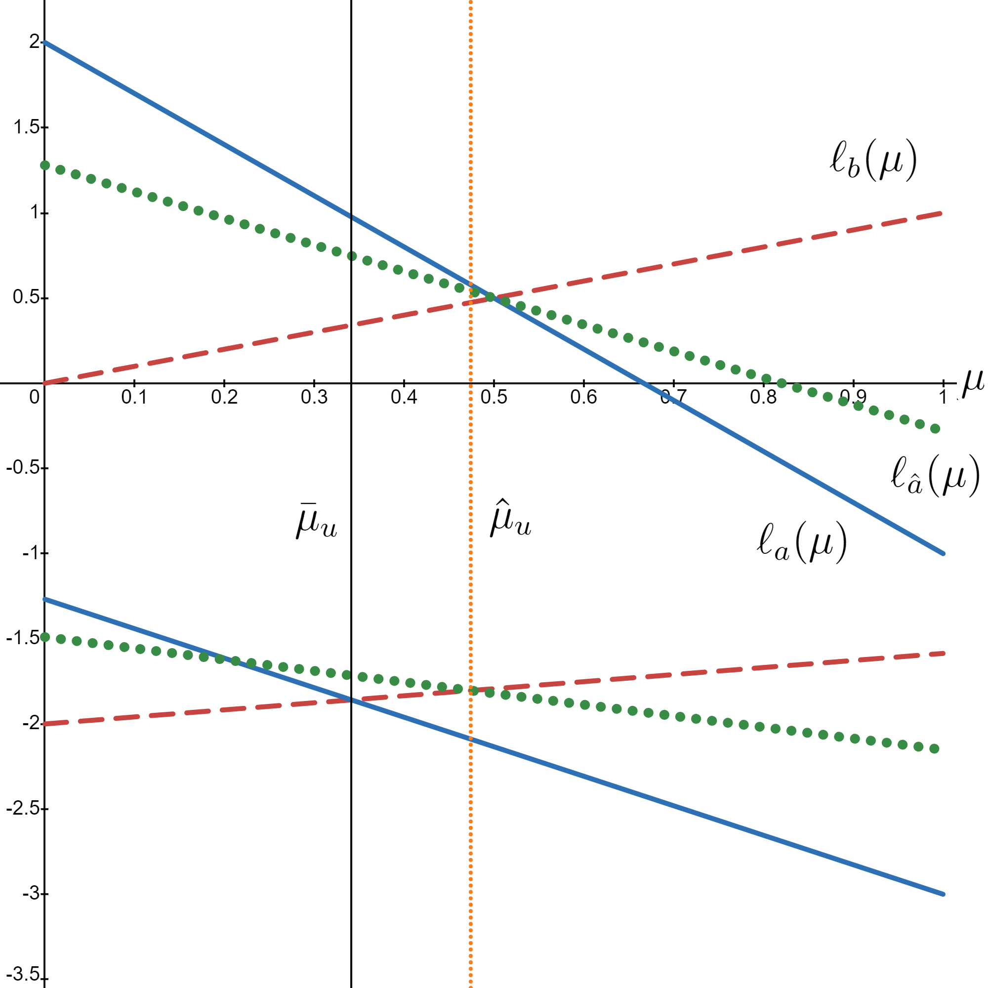
Another perspective on this theorem is a purely geometric one. Take the line, in belief ,
which is the expected payoff (in money) of action as a function of the belief . In turn, lines
are the expected payoffs to actions and , respectively. It turns out that -superiority of is equivalent to lying weakly above a counter-clockwise rotation of around the point , provided the rotation isn’t too extreme so that . When is a counter-clockwise rotation of , we have made it “more like ,” and this cannot hurt ’s comparative attractiveness versus .
Figure 1 illustrates the benefits of a counter-clockwise rotation. The top three lines are the expected payoffs, in belief , to , , and ; in dashed red, dotted green, and solid blue, respectively. The bottom three lines are the expected utilities (with ) to the three actions, maintaining the same color and fill correspondences. Line is in (thin) solid black and is in (thin) dotted orange. Here is an interactive link, where the line can be rotated by moving the slider. See how moves!
Before going on, let us jot down this informal discussion as a formal result.
Corollary 3.8.
is -superior to if and only if and there exists a such that lies weakly above the line .
So far we have assumed mild but meaningful structure on the DM’s utility function. More is better ( is strictly increasing in the reward), and the DM is risk-averse ( is, at least weakly, concave). Suppose we remove the assumption of risk aversion. We still assume that is strictly increasing but now allow it to take arbitrary shape.
As we now document, this is, in a sense, a step too far. Without the assumption of risk aversion, the only transformations that must make less attractive are unambiguous dominance improvements from to . This is intuitive: think back to Theorem 3.7. There, the necessary transformations were either dominance shifts (which obviously lead to be better versus than ) or spreads or contractions of , depending on the initial structure of the problem. However, the opposite modifications are needed when is convex–which is now permitted. Consequently, other than a dominance improvement, there is no way to ensure the desired outcome when the DM may be either risk loving or risk averse. Formally,
Theorem 3.9.
Action is -better than action if and only if and dominates or .
3.2 More Than Two States
Now let be an compact and metrizable space (endowed with the Borel -algebra). We partition into three sets:
We extend the earlier (two-state) definition of dominance:
Definition 3.10.
Action Dominates action if for all .
Then, for any pair and , let denote the binary distribution over states supported on only and at which the DM is indifferent between and , i.e.,
For any pair of states and , we define an X improvement–where X is either “consistent,” “inconsistent,” or “-state”–to be exactly as defined in the two-state setting (3.1), where state is replaced with , with , and with . Likewise, we extend the definition of “improvement,” so that is an improvement to if for any , , and for any and , and is either a consistent, an inconsistent, or a -state improvement to . Then,
Theorem 3.11.
is -superior to if and only if is an improvement to .
Proof.
We merely sketch the proof, as this theorem is proved identically to Theorem 3.4 in Pease and Whitmeyer (2023). The key observation is that () is a compact convex subset of whose extreme points are the degenerate probability distributions at which () is preferred to and the binary distributions at which the DM is indifferent between () and . By the Krein-Milman theorem, these sets of extreme points characterize the sets and , so the result is equivalent to the extreme points acting in a particular way (moving “away” from each along each edge of the simplex connecting and ) as we go from to . Hence, it is necessary and sufficient to simply aggregate the two-state result. ∎
This extreme points argument goes through without alteration to produce our second result.
Theorem 3.12.
Action is -better than action if and only if for all and dominates or .
Proof.
Omitted as the already-cited extreme-points argument is valid. ∎
4 One Versus Many
What if we look for improvements to that make it more attractive in comparison to multiple alternatives, not just a single one? For simplicity, we restrict our attention to the two-state environment. Let be the DM’s finite set of actions, where we assume that none are (strictly) dominated. Indexing the actions by a finite set (with ), we assume without loss of generality (as we could just relabel actions) that for all , and for all ().
There are two special actions, and . The first is uniquely optimal in state and the second is uniquely optimal in state . We term these the two extreme actions. For a specified , we define and
We define to be the analogous set with a strict inequality, and sets and their compatriots once we’ve replaced with .
Definition 4.1.
Action is -Superior to action if the set of beliefs at which the DM prefers to the actions other than , , is a subset of the set of beliefs at which the DM prefers to those other actions, ; and ; no matter the risk-averse agent’s utility function.
We have the following stark result.
Proposition 4.2.
If (), is -superior to if and only if is -superior to (). If is not one of the extreme actions, is -superior to if and only if dominates .
Proof.
Let (the proof for is identical). Observe that if , for all . By the monotonicity of the indifference points between the successive actions are increasing, i.e., the indifference point between and –if it exists–is (weakly) to the left of that between and , which is strictly to the left of that between and , etc.111For any strictly increasing the slopes of the lines are strictly increasing in , which implies this observation. If there is no indifference point between and , must be strictly dominated as a result of the transformation. But then it is obvious that the indifference point between and the lowest undominated () must be to the right of the indifference point between and . We conclude that if .
If it is immediate that dominating implies .
The logic behind this proposition is straightforward. For an action to improve versus the action to its right, we need the induced (risk-neutral) line in belief space to lie above some counterclockwise rotation around the indifference point between the two actions. For an action to improve versus the action to its left, we need the line in belief space to lie above the indifference point between the two actions (which is strictly to the left of the other indifference point). A dominance shift is the only way to reconcile these requirements.
5 Robustness to Aggregate Risk
What if the DM also has unknown (to us) random wealth? Formally, in any state , the DM’s utility from action is , where is a state-independent (finite-mean) random variable .
Abusing notation, we define to be the subset of for which is preferred to :
is this set’s strict-preference counterpart.
We extend our definitions in the natural way:
Definition 5.1.
Action is - and Wealth-Superior to action if the set of beliefs at which the DM prefers to , , is a subset of the set of beliefs at which the DM prefers to , ; and the set of beliefs at which the DM strictly prefers to , , is a subset of the set of beliefs at which the DM strictly prefers to , ; no matter the risk-averse agent’s utility function (for any strictly increasing, concave ) and no matter the agent’s state-independent random wealth (for any finite-mean, real-valued random variable ).
Definition 5.2.
Action is - and Wealth-Better than action if the set of beliefs at which the DM prefers to , , is a subset of the set of beliefs at which the DM prefers to , ; and the set of beliefs at which the DM strictly prefers to , , is a subset of the set of beliefs at which the DM strictly prefers to , ; no matter the (not necessarily risk-averse) agent’s utility function (for any strictly increasing, concave ) and no matter the agent’s state-independent random wealth (for any finite-mean, real-valued random variable ).
Then,
Theorem 5.3.
is - and wealth-superior to if and only if is an improvement to . is - and wealth-better than if and only if for all and dominates or .
6 Everything Everywhere All at Once
In this paper, we focus on altering a single action, leaving the other action (or actions) unaltered. This is reasonable in many situations–for example, in the two applications in the next section, the other action is the DM’s outside option, which is unalterable. But what if we change both actions and ? As we will see, the basic intuition from the earlier results remains true, though we only provide a partial analysis, primarily to get bogged down in a tedium of cases. We also restrict attention to the two-state environment, as we could just follow the earlier approach to generate the result for a general state space (it will again just be the aggregation of the two-state conditions).
Now, we are going from to and to some . To that end, we define
understanding to be this set’s strict inequality counterpart.
Definition 6.1.
Given and , action is -Superior to action if, no matter the risk-averse agent’s utility function,
-
1.
and
-
2.
i.e., the set of beliefs at which the DM prefers to is a subset of the beliefs at which the DM prefers to .
It is easy to obtain an analogous inequality to Inequality 3.1, which is necessary for -superiority when :
Obviously, dominating or and being dominated by or imply -superiority. Here is a less obvious sufficient condition.
Proposition 6.2.
If Inequality 6 holds, , and , is -superior to action .
As we discussed above, improving upon versus (when is fixed) is equivalent to ’s expected payoff in belief space lying above a counter-clockwise rotation of ’s payoff. When we alter both actions, the rotation point may now shift–think vaguely of a co-movement of payoffs to both and –and ’s payoff and ’s payoffs are both counter-clockwise rotations about this point.
7 Applications
7.1 Robustly Optimal Bilateral Trade Modifications
There is a buyer () and a seller (). possesses an asset that pays out in state and in state . The state is contractible and the status quo trade agreement sees transfers of size from to in each state . We assume that and .
’s payoff from transacting is in state and in state . Similarly, ’s payoff from transacting is in state and in state . ’s outside option is the sure-thing and ’s outside option is the asset, with random payoff in state and in state .
We suppose that the status-quo is acceptable–given the agents’ subjective beliefs about uncertainty and their (concave) utility functions, each is willing to participate in the arrangement. What modifications to the arrangement are robustly optimal in that and will still remain willing to participate?
Observe that if and are risk-neutral, their indifference belief is
and () trades whenever she is sufficiently pessimistic (optimistic). Furthermore, in any modification, it is clear that Inequality 3.1 must hold with equality for both and , as transfers must balance. There are two cases to consider: 1. , and 2. .
Case 1. Suppose . By Lemma 3.4, a monotone alteration to the trade agreement–one that is such that –is acceptable to if and only it is a spread of the initial agreement:
Similarly, a monotone alteration–one that is such that –is acceptable to if and only if it is a contraction of the initial agreement, which corresponds to the conditions in Expression 7.1. By Lemma 3.5, there is no (robustly) acceptable non-monotone alteration.
Remark 7.1.
If , the set of acceptable alterations are monotone and satisfy the conditions in Expression 7.1.
Case 2. Now suppose . Now, the only monotone alteration to the trade agreement acceptable to is a contraction of the initial agreement:
As before, the only monotone alteration is guaranteed to accept is a contraction, so Expression 7.1 specifies the binding constraints.
Finally, Lemma 3.5 implies that and will accept any non-monotone alteration (that preserves the expected value) and strict optimality in state and , respectively:
7.2 Robustly Optimal Insurance Modifications
Now consider the scenario of a risk-neutral insurer and a consumer. The consumer’s payoff without insurance is in state and in state . The status-quo insurance policy pays out to the consumer in state and () in state . We assume further that . Thus, if the consumer buys the status-quo contract, she gets in state and in state . In contrast, if she does not buy insurance, she gets and in the two states, respectively.
The consumer’s (risk-neutral) indifference belief is
A new contract is acceptable if the consumer is willing to accept it, given that she is willing to accept the status-quo contract, no matter her concave utility function or prior. Appealing to Lemma 3.5, we have
Remark 7.3.
If the new contract is such that , , and , the new contract is acceptable.
References
- Athey (2002) Susan Athey. Monotone comparative statics under uncertainty. The Quarterly Journal of Economics, 117(1):187–223, 2002.
- Aumann and Serrano (2008) Robert J Aumann and Roberto Serrano. An economic index of riskiness. Journal of Political Economy, 116(5):810–836, 2008.
- Bali et al. (2011) Turan G Bali, Nusret Cakici, and Fousseni Chabi-Yo. A generalized measure of riskiness. Management science, 57(8):1406–1423, 2011.
- Battigalli et al. (2016) Pierpaolo Battigalli, Simone Cerreia-Vioglio, Fabio Maccheroni, and Massimo Marinacci. A note on comparative ambiguity aversion and justifiability. Econometrica, 84(5):1903–1916, 2016.
- Choi and Smith (2017) Michael Choi and Lones Smith. Ordinal aggregation results via karlin’s variation diminishing property. Journal of Economic theory, 168:1–11, 2017.
- Curello and Sinander (2019) Gregorio Curello and Ludvig Sinander. The preference lattice. Mimeo, 2019.
- Edlin and Shannon (1998) Aaron S Edlin and Chris Shannon. Strict single crossing and the strict spence-mirrlees condition: a comment on monotone comparative statics. Econometrica, 66(6):1417–1425, 1998.
- Foster and Hart (2009) Dean P Foster and Sergiu Hart. An operational measure of riskiness. Journal of Political Economy, 117(5):785–814, 2009.
- Hammond III (1974) John S Hammond III. Simplifying the choice between uncertain prospects where preference is nonlinear. Management Science, 20(7):1047–1072, 1974.
- Jewitt (1987) Ian Jewitt. Risk aversion and the choice between risky prospects: the preservation of comparative statics results. The Review of Economic Studies, 54(1):73–85, 1987.
- Jewitt (1989) Ian Jewitt. Choosing between risky prospects: the characterization of comparative statics results, and location independent risk. Management Science, 35(1):60–70, 1989.
- Karlin and Novikoff (1963) Samuel Karlin and Albert Novikoff. Generalized convex inequalities. Pacific Journal of Mathematics, 13(4), 1963.
- Kartik et al. (2023) Navin Kartik, SangMok Lee, and Daniel Rappoport. Single-crossing differences in convex environments. Review of Economic Studies, page rdad103, 2023.
- Lambert and Hey (1979) Peter J Lambert and John D Hey. Attitudes to risk. Economics Letters, 2(3):215–218, 1979.
- Milgrom and Shannon (1994) Paul Milgrom and Chris Shannon. Monotone comparative statics. Econometrica, pages 157–180, 1994.
- Pease and Whitmeyer (2023) Marilyn Pease and Mark Whitmeyer. Safety, in numbers. Mimeo, 2023.
- Phelps (2009) Robert R Phelps. Convex functions, monotone operators and differentiability, volume 1364. Springer, 2009.
- Quah and Strulovici (2012) John K-H Quah and Bruno Strulovici. Aggregating the single crossing property. Econometrica, 80(5):2333–2348, 2012.
- Riedel and Hellmann (2015) Frank Riedel and Tobias Hellmann. The foster–hart measure of riskiness for general gambles. Theoretical Economics, 10(1):1–9, 2015.
- Rothschild and Stiglitz (1970) Michael Rothschild and Joseph E Stiglitz. Increasing risk: I. a definition. Journal of Economic Theory, 2(3):225–243, 1970.
- Weinstein (2016) Jonathan Weinstein. The effect of changes in risk attitude on strategic behavior. Econometrica, 84(5):1881–1902, 2016.
Appendix A Omitted Proofs
A.1 Lemma 3.4 Proof
Proof.
If and dominates , the result is trivial. So, suppose that and . First, let . It suffices to show the result when is a MPC of , as subsequent dominance can only improve ’s attractiveness in relation to . Moreover, we may also assume and , i.e., . This implies that .
There are two cases: either 1. is such that , or 2. is such that .
Case 1. As the line (in belief space) corresponding to crosses the line corresponding to from above and , it must be that
Moreover, in the terminology of Pease and Whitmeyer (2023), is safer than , so
where the last line follows from the definition of . Consequently, the DM prefers to for all , strictly so for all .
Case 2. Suppose now that , and suppose for the sake of contradiction that
But, as and , this implies that is strictly dominated when the DM has utility , contradicting the two Proposition 1s in Weinstein (2016) and Battigalli, Cerreia-Vioglio, Maccheroni, and Marinacci (2016), which state that an increase in risk aversion cannot shrink the set of undominated actions.
Now let . As before, it suffices to show the result when is a MPS of , as subsequent dominance can only improve ’s attractiveness in relation to . This implies
Consequently,
where the first inequality follows from the Three-chord lemma (Theorem 1.16 in Phelps (2009)), the second inequality from Inequality 3.1, and the third inequality from the Three-chord lemma.
It is obvious that is necessary, so we assume it to hold. First, let and suppose for the sake of contraposition that neither dominates nor a MPC of . This implies that . Moreover, if Inequality 3.1 does not hold we are also done, so we assume that it does hold. This implies that and .
We want to find a concave, strictly increasing such that . Here is one:
for some . Directly, equals
This expression is continuous and decreasing in and is strictly positive when . Accordingly for all sufficiently small , we have that .
Now let and suppose for the sake of contraposition that neither dominates nor a MPS of . Again, this implies and that or . As we may assume Inequality 3.1 holds, it cannot be that both hold, which means that and . Consequently, by monotonicity of the transformation, we must have
Let
for some . Directly, equals
which is strictly positive when .∎
A.2 Lemma 3.5 Proof
Proof.
Let . If and , the result is immediate. Likewise, if , dominates , which yields the result.
Now suppose , , and Inequality 3.1 holds. Fix . By the non-monotonicity of the transformation
viz., is safer than . Furthermore, this means that there exists a such that the DM prefers to for all , strictly so for . As Inequality 3.1 holds and , . This implies that there exists such that the DM prefers to for all strictly so for .
As cannot be strictly dominated (appealing to the Proposition 1s in Weinstein (2016) and Battigalli et al. (2016)), . Consequently, .
If , this direction is immediate, as dominance over or makes relatively more attractive versus than is.
If , this direction is immediate.
So, let . We assume or else the result is immediate. Suppose for the sake of contradiction that neither dominates nor . This implies that . As does not dominate it must be that or else we would have . We assume that Inequality 3.1 holds, or else we are done. This means that . Summarizing things, we have
The location of is ambiguous with respect to , but that won’t matter.
Let
for some in which case equals
which is strictly positive when .∎
A.3 Lemma 3.6 Proof
Proof.
Let . If Condition 1 holds, the result is obvious. So, suppose Condition 2 holds instead. If dominates , we are done, so let that not be the case. This means that (as Inequality 3.1 holds)
Then, the chain of inequalities in Expression A.1 is valid, yielding the result.
It suffices (as the other cases are trivial) to assume that , , and Inequality 3.1 hold, and to suppose for the sake of contraposition that .
Take
for some , so that equals
which is strictly positive when .∎
A.4 Theorem 3.9 Proof
Proof.
This direction is trivial.
Let . We suppose for the sake of contraposition that and that does not dominate . We also assume that Inequality 3.1 holds, or else the result is immediate. This means that either 1. and or 2. and .
Case 1. First suppose so that we have the chain
Take
for some , so that equals
which is strictly positive when .
Now suppose , in which case we have
The same defined in Expression A.4 will do. Thus, equals
If , this equals
when . If , it equals
when .
Case 2. First suppose so that we have the chain
Take
for some , so that equals
which is strictly positive when .
Now suppose , in which case we have
Using the from Expression A.4, equals
If , this equals
when . If , this equals
when . ∎
A.5 Theorem 5.3 Proof
Proof.
The second sufficiency statement is also immediate. Let us tackle the first. We specify–appealing to the aggregation argument from Theorem 3.7–that there are two states, i.e., . We also assume (as the other cases are easy) that doesn’t dominate , and that is strictly preferred to in state and vice-versa in state .
We prove a sequence of lemmas. We note that and remain unchanged (the aggregate risk cancels out), but redefine
and
Lemma A.1.
Suppose the transformation from to is monotone. Then,
-
1.
If , is - and wealth-superior to if dominates a MPC of .
-
2.
If , is - and wealth-superior to if dominates a MPS of .
Proof.
We follow the proof of Lemma 3.4. There are two cases: either 1. is such that , or 2. is such that .
Case 1. As and , it must be that
Moreover, in the terminology of Pease and Whitmeyer (2023), hedges risk better than , so (by Proposition 6.2 in that paper), and defining ,
where the last line follows from the definition of . Consequently, the DM prefers to for all , strictly so for all .
Case 2. Suppose now that , and suppose for the sake of contradiction that
But, as and , this implies that is strictly dominated when the DM has utility . We need to show that this cannot happen.
Claim A.2.
is not strictly dominated when the DM has concave utility .
Proof.
Appealing to the Wald-Pearce lemma, suppose there exists a such that for all
Observe that the function is concave. Accordingly, for all
But as is undominated for a risk-neutral DM, for this , there exists a such that
Combining these inequalities, we get that for some ,
a contradiction. ∎
Now let . As before, it suffices to show the result when is a MPS of , as subsequent dominance can only improve ’s attractiveness in relation to . This implies
Consequently, the chain of inequalities in Expression A.1 can be replicated, replacing function with .∎
Lemma A.3.
Suppose the transformation from to is non-monotone. is - and wealth-superior to if , , and Inequality 3.1 holds.
Proof.
Finally,
Lemma A.4.
Let . Then, is - and wealth-superior to if and Inequality 3.1 holds.
Proof.
Replicate the chain of inequalities in Expression A.1, replacing function with . ∎
This completes the proof of the theorem. ∎