On the Impact of Predictor Serial Correlation on the LASSO

Abstract

We explore inference within sparse linear models, focusing on scenarios where both predictors and errors carry serial correlations. We establish a clear link between predictor serial correlation and the finite sample performance of the LASSO, showing that even orthogonal or weakly correlated stationary AR processes can lead to significant spurious correlations due to their serial correlations. To address this challenge, we propose a novel approach named ARMAr-LASSO (ARMA residuals LASSO), which applies the LASSO to predictor time series that have been pre-whitened with ARMA filters and lags of dependent variable. Utilizing the near-epoch dependence framework, we derive both asymptotic results and oracle inequalities for the ARMAr-LASSO, and demonstrate that it effectively reduces estimation errors while also providing an effective forecasting and feature selection strategy. Our findings are supported by extensive simulations and an application to real-world macroeconomic data, which highlight the superior performance of the ARMAr-LASSO for handling sparse linear models in the context of time series.

Keywords: Time series, serial correlation, spurious correlation, LASSO.

1 Introduction

The LASSO (Tibshirani, 1996) is perhaps the most commonly employed approach to handle regressions with a large number of predictors. From a theoretical standpoint, its effectiveness in terms of estimation, prediction, and feature selection is contingent upon either orthogonality or reasonably weak correlation among predictors (see Zhao and Yu 2006; Bickel et al. 2009; Negahban et al. 2012; and Hastie 2015). This hinders the use of the LASSO for the analysis of economic time series data, which are notoriously characterized by intrinsic multicollinearity; that is, by predictor correlations at the population level (Forni et al., 2000; Forni and Lippi, 2001; Stock and Watson, 2002a; De Mol et al., 2008; Medeiros and F.Mendes, 2012). A common procedure to address this issue is to model multicollinearity and remove it, as proposed, e.g., by  Fan et al. (2020), who filter time series using common factors and then apply the LASSO to the filtered residuals. However, mitigating or even eliminating multicollinearity is not the end of the story, as effectiveness of the LASSO can also be affected by spurious correlations. These occur when predictors are orthogonal or weakly correlated at the population level, but a lack of sufficient independent replication (lack of degrees of freedom) introduces correlations at the sample level, potentially leading to false scientific discoveries and incorrect statistical inferences (Fan and Zhou, 2016; Fan et al., 2018). This issue has been broadly explored in ultra-high dimensional settings, where the number of predictors can vastly exceed the available sample size (Fan et al., 2014). We argue that in time series data, lack of independent replication can be due not only to a shortage of available observations but also to serial correlation.

This article introduces two elements of novelty. First, we establish an explicit link between serial correlations and spurious correlations. At a theoretical level, we derive the density of the sample correlation between two orthogonal stationary Gaussian AR(1) processes, and show how such density depends not only on the sample size but also on the degree of serial correlation; at any given sample size, an increase in serial correlation results in a larger probability of sizable spurious correlations. Then we use extensive simulations to show how this dependence holds in much more general settings (e.g., when the underlying processes are not orthogonal, or non Gaussian ARMA).

Second, we propose an approach that, using a filter similar to that proposed by Fan et al. (2020), rescues the performance of the LASSO in the presence of serially correlated predictors. Our approach, which we name ARMAr-LASSO (ARMA residuals LASSO), relies upon a working model where, instead of the observed predictor time series, we use as regressors the residuals of ARMA processes fitted on such series, augmented with lags of the dependent variable. We motivate our choice of working model and provide some asymptotic arguments concerning limiting distribution and feature selection consistency. Subsequently, we employ the mixingale and near-epoch dependence framework (Davidson, 1994; Adamek et al., 2023) to prove oracle inequalities for the estimation and forecast error bounds of the ARMAr-LASSO, while simultaneously addressing the issue of estimating ARMA residuals. To complete the analysis, we use simulations to validate and generalize the theoretical result. Furthermore, we apply our methodology to a high-dimensional dataset for forecasting the consumer price index in the Euro Area. Simulations and empirical exercises demonstrate that the ARMAr-LASSO produces more parsimonious models, better coefficient estimates, and more accurate forecasts than LASSO-based methods applied to time series. Notably, both theoretical and numerical results concerning our approach hold even in contexts of factor-induced multicollinearity, provided that the idiosyncratic components are orthogonal or weakly correlated processes exhibiting serial correlation. Code and replicability material is available at https://doi.org/10.5281/zenodo.13335323.

Our work complements the vast literature on error bounds for LASSO-based methods in time series analysis, which addresses estimation and forecast consistency in scenarios with autocorrelated errors and autoregressive processes (Bartlett, 1935; Granger and Newbold, 1974; Granger et al., 2001; Hansheng Wang and Jiang, 2007; Wang et al., 2007; Hsu et al., 2008; Nardi and Rinaldo, 2011; Chronopoulos et al., 2023; Baillie et al., 2024). Moreover, our methodology aligns with the prevailing literature on pre-whitening filters, which are commonly employed to mitigate autocorrelation in the error component or to enhance cross-correlation analysis. For instance, Robinson (1988) suggests obtaining residuals from partial linear models and then applying least squares to estimate a non-parametric component. Belloni et al. (2013) propose a similar approach in high-dimensional settings, using LASSO on the residuals from a parametric component. Hansen and Liao (2019) show that, in panel data model inference, applying a PCA filter to eliminate multicollinearity and using LASSO on its residuals can produce reliable confidence intervals. Finally, as mentioned, Fan et al. (2020) illustrate how latent factors create strong dependencies among regressors, complicating feature selection, while selection improves on idiosyncratic components.

The remainder of the article is organized as follows. Section 2 introduces the problem setup and our results concerning the link between serial correlations and spurious correlations. Section 3 introduces the ARMAr-LASSO and explores its theoretical properties. Section 4 presents simulations and real data analyses to evaluate the performance of our proposed methodology. Section 5 provides some final remarks.

We summarize here some notation that will be used throughout. Bold letters denote vectors, for example $\mathbf{a}=(a_{1},\dots,a_{p})^{\prime}$. Supp$(\mathbf{a})$ denotes the support of a vector, that is, $\{i\in\{1,\dots,p\}:a_{i}\neq 0\}$, and $|\text{Supp}(\mathbf{a})|$ the support cardinality. The $\ell_{q}$ norm of a vector is $||\mathbf{a}||_{q}\coloneqq\mathopen{}\mathclose{{}\left(\sum_{j=1}^{p}|a_{j}|^{q}}\right)^{1/q}$ for $0<q<\infty$, with $||\mathbf{a}||_{q}^{k}\coloneqq\mathopen{}\mathclose{{}\left(\sum_{j=1}^{p}|a_{j}|^{q}}\right)^{k/q}$, and with the usual extension $||\mathbf{a}||_{0}\coloneqq|\text{Supp}(\mathbf{a})|$. Bold capital letters denote matrices, for example $\mathbf{A}$, where $\mathopen{}\mathclose{{}\left(\mathbf{A}}\right)_{ij}=a_{ij}$ is the $i$-row $j$-column element. Furthermore, $\boldsymbol{0}_{p}$ denotes a $p$-length vector of zeros, $\boldsymbol{I}_{p}$ the $p\times p$ identity matrix, and $\text{Sign}(r)$ the sign of a real number $r$. To simplify the analysis, we frequently make use of arbitrary positive finite constants $C$.

2 Problem Setup

Consider the linear regression model

$$y_{t}=\mathbf{x}_{t}^{\prime}\boldsymbol{\alpha}^{*}+\varepsilon_{t}\ \ ,\ \ \ \ \ \ t=1,\ldots,T\ \ ,$$ (1)

where $\mathbf{x}_{t}=(x_{1,t},\ldots,x_{n,t})^{\prime}$ is a $n\times 1$ vector of predictors, $\boldsymbol{\alpha}^{*}$ is a $n\times 1$ unknown $s$-sparse vector of regression coefficients, i.e. $||\boldsymbol{\alpha}^{*}||_{0}=s<n$, and $\varepsilon_{t}$ is an error term. We impose the following assumptions on the processes $\mathopen{}\mathclose{{}\left\{\mathbf{x}_{t}}\right\}$ and $\mathopen{}\mathclose{{}\left\{\varepsilon_{t}}\right\}$.

Assumption 1:

$\mathopen{}\mathclose{{}\left\{\mathbf{x}_{t}}\right\}$ and $\mathopen{}\mathclose{{}\left\{\varepsilon_{t}}\right\}$ are non-deterministic second order stationary processes.

Under Assumption 1, the predictors and the error terms are weakly stationary and admit an ARMA representation of the form

$$x_{i,t}=\sum_{l=1}^{p_{i}}\phi_{i,l}x_{i,t-l}+\sum_{k=1}^{q_{i}}\theta_{i,k}u_{i,t-k}+u_{i,t}\ \ ,\ \ \ \ \ \ i=1,\dots,n\ \ ,$$ (2)

$$\varepsilon_{t}=\sum_{l=1}^{p_{\varepsilon}}\phi_{\varepsilon,l}\varepsilon_{t-l}+\sum_{k=1}^{q_{\varepsilon}}\theta_{\varepsilon,k}\omega_{t-k}+\omega_{t}\ \ ,$$ (3)

where the innovation processes $u_{i,t}\sim w.n.(0,\sigma_{i}^{2})$, $\omega_{t}\sim w.n.(0,\sigma_{\omega}^{2})$ are sequences of zero-mean white noise ($w.n.$) with finite variances (see Reinsel 1993, ch. 1.2 for details).

Assumption 2:

$u_{i,t}\perp u_{j,t-l}$ for any $i\neq j,t$ and $l\neq 0$; and $u_{i,t-l}\perp\omega_{t}$ for any $i,t$ and $l$.

There are several approaches to estimate $\boldsymbol{\alpha}^{*}$ when $n$ is comparable to or larger than $T$ (Zhang and Zhang, 2012; James et al., 2013); here we focus on the LASSO estimator (Tibshirani, 1996) given by $\widehat{\boldsymbol{\alpha}}=\underset{\boldsymbol{\alpha}\in\mathbb{R}^{n}}{\operatornamewithlimits{argmin\ }}\>\mathopen{}\mathclose{{}\left\{\frac{1}{2T}||\mathbf{y}-\mathbf{X}^{\prime}\boldsymbol{\alpha}||_{2}^{2}+\lambda||\boldsymbol{\alpha}||_{1}}\right\},$ where $\lambda>0$ is the weight of the $\ell_{1}$ penalty and must be “tuned” to guarantee that regression coefficient estimates are effectively shrunk to zero – thus ensuring predictor, or feature, selection.

However, linear associations among predictors are well known to affect LASSO performance. Bickel et al. (2009); Bühlmann and van de Geer (2011) and Negahban et al. (2012) have shown that the LASSO estimation and prediction accuracy are inversely proportional to the minimum eigenvalue of the predictor sample covariance matrix. Thus, highly correlated predictors deteriorate estimation and prediction performance. Moreover,  Zhao and Yu (2006) proved that the LASSO struggles to differentiate between relevant (i.e., $\{i\in\{1,\dots,n\}:\alpha_{i}^{*}\neq 0\}$) and irrelevant (i.e., $\{i\in\{1,\dots,n\}:\alpha_{i}^{*}=0\}$) predictors when they are closely correlated, leading to false positives. Thus, highly correlated predictors may also deteriorate feature selection performance. The weak irrepresentable condition addresses this issue ensuring both estimation and feature selection consistency through bounds on the sample correlations between relevant and irrelevant predictors (Zhao and Yu 2006, see also Bühlmann and van de Geer 2011). Nevertheless, orthogonality or weak correlation seldom hold in the context of economic and financial data. For instance, decades of literature provide evidence for co-movements of macroeconomic variables (Forni et al., 2000; Forni and Lippi, 2001; Forni et al., 2005; Stock and Watson, 2002a, b). Special methods have been proposed to mitigate the negative effects of these linear associations, such as Factor-Adjusted Regularized Model Selection (FarmSelect) (Fan et al., 2020), which applies the LASSO to the idiosyncratic components of economic variables, obtained by filtering the variables through a factor model. Although approaches such as FarmSelect can be very effective in addressing multicollinearity, strong spurious correlations can emerge at the sample level and affect the LASSO even when predictors are orthogonal or weakly correlated at the population level. This is the case for large regressions, where the number of predictors is comparable to or even larger than the sample size, and even more so for large regressions involving time series, where independent replication can be further hindered by serial correlations. This article focuses specifically on spurious sample-level correlations; in the next section, we introduce a theoretical result linking serial correlations within time series to the sample correlations between them.

2.1 Serial and Sample Correlations for Time Series

Consider a first order $n$-variate autoregressive process $\mathbf{x}_{t}=\boldsymbol{\phi}^{\prime}\mathbf{x}_{t-1}+\mathbf{u}_{t}$, $t=1,\dots,T$, where $\boldsymbol{\phi}=(\phi_{1},\dots,\phi_{n})^{\prime}$ are autoregressive coefficients such that $|\phi_{i}|<1$ for each $i=1,\dots,n$, and $\mathbf{u}_{t}\sim N\mathopen{}\mathclose{{}\left(\boldsymbol{0}_{n},\boldsymbol{I}_{n}}\right)$. Assume that each $\mathbf{x}_{i}$ is standardized so that $\frac{1}{T-1}\sum_{t}x_{i,t}=0$ and $\frac{1}{T}\sum_{t}x_{i,t}^{2}=1$, and let $\widehat{\mathbf{C}}_{x}=\frac{1}{T}\mathbf{X}\mathbf{X}^{\prime}$ be the sample covariance, or equivalently, correlation matrix – with generic off-diagonal element $\widehat{c}_{ij}^{x}$ and eigenvalues $\widehat{\psi}_{max}^{x}\geq\ldots\geq\widehat{\psi}_{min}^{x}$. Here $\mathbf{x}_{t}\sim$ $N\mathopen{}\mathclose{{}\left(\boldsymbol{0}_{n},\mathbf{C}_{x}}\right)$ with $\mathopen{}\mathclose{{}\left(\mathbf{C}_{x}}\right)_{ii}=\frac{1}{1-\phi_{i}^{2}}$, and $\mathopen{}\mathclose{{}\left(\mathbf{C}_{x}}\right)_{ij}={c}_{ij}^{x}=0$, for $i\neq j$. Our next task is to link $\Pr\mathopen{}\mathclose{{}\left(|\widehat{c}_{ij}^{x}|\geq\tau}\right)$, $\tau\in[0,1)$, to serial correlations. To this end, the following theorem provides an approximation for the density of the sample correlation coefficient.

Theorem 1:

Let $\{\mathbf{x}_{t}\}$ be a stationary $n$-variate Gaussian AR(1) process with autoregressive residuals $\mathbf{u}_{t}\sim N\mathopen{}\mathclose{{}\left(\boldsymbol{0}_{n},\boldsymbol{I}_{n}}\right)$. Let $\ddot{\phi}=\phi_{i}\phi_{j}$, where $\phi_{i}$ and $\phi_{j}$ are the autoregressive coefficients of the $i$-th and $j$-th processes, respectively. Then, the density of $\widehat{c}_{ij}^{x}$ is approximated by

$$\small\mathcal{D}_{\widehat{c}_{ij}^{x}}=\frac{\Gamma\mathopen{}\mathclose{{}\left(\frac{T-1}{2}}\right)(1-\ddot{\phi})}{\Gamma\mathopen{}\mathclose{{}\left(\frac{T-2}{2}}\right)\sqrt{\pi}}(1-(\widehat{c}_{ij}^{x})^{2})^{\frac{T-4}{2}}\mathopen{}\mathclose{{}\left(1-\ddot{\phi}^{2}}\right)^{\frac{T-2}{2}}\mathopen{}\mathclose{{}\left(\frac{1}{1-\ddot{\phi}^{2}+2(\widehat{c}_{ij}^{x})^{2}\ddot{\phi}(\ddot{\phi}-1)}}\right)^{\frac{T-1}{2}}.$$

Proof: see Supplement B.1

Theorem 1 shows that, in a finite sample setting, the density $\mathcal{D}_{\widehat{c}_{ij}^{x}}$ and thus the probability $\Pr\mathopen{}\mathclose{{}\left(|\widehat{c}_{ij}^{x}|\geq\tau}\right)\approx\int_{-1}^{-\tau}\mathcal{D}_{\widehat{c}_{ij}^{x}}d\widehat{c}_{ij}^{x}+\int_{\tau}^{1}\mathcal{D}_{\widehat{c}_{ij}^{x}}d\widehat{c}_{ij}^{x}$ of observing sizable spurious correlations between two orthogonal Gaussian autoregressive processes, depends on their degrees of serial correlation, i.e., on both the magnitude and the sign of $\ddot{\phi}=\phi_{i}\phi_{j}$. When $Sign(\phi_{i})=Sign(\phi_{j})$, an increase in $|\ddot{\phi}|$ results in a density with thicker tails, and thus a higher $\Pr\mathopen{}\mathclose{{}\left(|\widehat{c}_{ij}^{x}|\geq\tau}\right)$. This, in turn, leads to a higher probability of a small minimum eigenvalue (as a consequence of the inequality $\Pr\mathopen{}\mathclose{{}\left(\widehat{\psi}_{min}^{x}\leq 1-\tau}\right)\geq\Pr\mathopen{}\mathclose{{}\left(|\widehat{c}_{ij}^{x}|\geq\tau}\right)$; see Supplement A for details), and a higher chance of breaking the irrepresentable condition if, say, one of the processes is relevant for the response and the other is not ($\alpha_{i}^{*}\neq 0$ and $\alpha_{j}^{*}=0$, or vice versa). When $Sign(\phi_{i})\neq Sign(\phi_{j})$, an increase in $|\ddot{\phi}|$ results in a density more concentrated around the origin. In Supplement C we provide an extensive numerical validation of Theorem 1, investigating the impact of the sign of $\ddot{\phi}$, as well as more realistic scenarios with correlated, non-Gaussian, and/or ARMA processes, through multiple simulation experiments.

We conclude this Section with a simple “toy experiment”. We generate data for $t=1,\dots,T$ from a $10$-variate process $\mathbf{x}_{t}=\boldsymbol{\phi}^{\prime}\mathbf{x}_{t-1}+\mathbf{u}_{t}$, where all components share the same autoregressive coefficient $\phi_{i}=\phi$, $i=1,\ldots,10$, and $\mathbf{u}_{t}\sim N\mathopen{}\mathclose{{}\left(\boldsymbol{0}_{10},\boldsymbol{I}_{10}}\right)$. Because of orthogonality, the maximum off-diagonal element and the minimum eigenvalue of the population correlation matrix $\mathbf{C}_{x}$ are, respectively, $\underset{i\neq j}{\text{max}}|c_{ij}^{x}|=0$ and $\psi_{min}^{x}=1$. We consider $\phi=0.0,0.3,0.6,0.9,0.95$, and $T=100,250$. For each scenario we calculate the average and standard deviation of $\underset{i\neq j}{\text{max}}|\widehat{c}_{ij}^{x}|$ and $\widehat{\psi}_{min}^{x}$ over 5000 Monte Carlo replications. Results are shown in Figure 1; a stronger persistence (higher $\phi$) increases the largest spurious sample correlations and decreases the smallest eigenvalue. However, as expected, an increase in the sample size from $T=100$ (panel (a)) to $T=250$ (panel (b)), reduces the impact of $\phi$. For example, the values of $\underset{i\neq j}{\text{max}}|\widehat{c}_{ij}^{x}|$ and $\widehat{\psi}_{min}^{x}$ in the case of $T=100$ and $\phi=0.6$ are quite similar to those obtained for $T=250$ and $\phi=0.9$.

(a)

(b)

Figure 1: Results from a numerical “toy example”. Panel (a) $T=100$, Panel (b) $T=250$. Orange circles/bars and blue triangles/bars represent, respectively, means/standard deviations of $\max_{i\neq j}|\widehat{c}_{ij}^{x}|$ and $\widehat{\psi}_{min}^{x}$, for various values of the autoregressive coefficient $\phi$, as obtained from 5000 Monte Carlo replications.

Note that these results are valid for any type of orthogonal or weakly correlated predictors, as long as they carry serial correlations. These predictors can be either directly observed variables or, for example, factor model residuals.

3 The ARMAr-LASSO

We now switch to describing ARMAr-LASSO (ARMA residuals LASSO), the approach that we propose to rescue LASSO performance in the presence of serially correlated predictors. ARMAr-LASSO is formulated as a two-step procedure. In the first step we estimate a univariate ARMA model on each predictor. In the second step, we run the LASSO using, instead of the original predictors, the residuals from the ARMA model, i.e., estimates of the $u$’s in equation (2), plus one or more lags of the response. We start by introducing the “working model” on which our proposal relies; that is, the model that contains the true (not observable) ARMA residuals (their estimation will be addressed later)

$$y_{t}=\mathbf{w}_{t}^{\prime}\boldsymbol{\beta}^{*}+v_{t}\ \ .$$ (4)

Model (4) is the linear projection of $y_{t}$ on $\mathbf{w}_{t}=(u_{1,t},\dots,u_{n,t},y_{t-1},\dots,y_{t-p_{y}})$, which contains $n$ ARMA residuals and $p_{y}$ lagged values of the response. $\boldsymbol{\beta}^{*}=\mathopen{}\mathclose{{}\left(\boldsymbol{\alpha}^{*^{\prime}},\phi_{y,1},\dots,\phi_{y,p_{y}}}\right)^{\prime}$ represents the corresponding best linear projection coefficients and $v_{t}$ is the error term, which is unlikely to be a white noise. It should be noted that the choice of $p_{y}$ is arbitrary and that some lags will be relevant while others will not. The relevant lags will be directly selected using LASSO. Model (4) is misspecified, in the sense that it does not correspond to the true data generating process (DGP) for the response, but it is similar in spirit to the factor filter used in the literature to mitigate multicollinearity (Fan et al., 2020). The idea behind model (4) is to leverage the serial independence of the $u$ terms, thereby avoiding the risk of sizable spurious correlation. However, the $u$ terms alone may explain only a small portion of the variance of $y_{t}$, particularly in situations with high persistence. This is why we introduce the response lags as additional predictors; these amplify the signal in our model and consequently improve the forecast of $y_{t}$. We list some important facts that capture how misspecification affects coefficient estimation and feature selection.

Fact 1:

(on the ARMA residuals) ($i$) $E(v_{t}|\mathbf{u}_{t})=0$; ($ii$) $E(\mathbf{u}_{t}y_{t-l})=\boldsymbol{0}$, $\forall$ $l\geq 1$, and $E(u_{it}y_{t-l}|u_{it-1}y_{t-l-1},u_{it-2}y_{t-l-2},\dots)=0$, $\forall$ $i,j\geq 1$.

Fact 1 follows from Assumptions 1 and 2. Fact 1 ($i$) ensures that the least square estimator of $\boldsymbol{\alpha}^{*}$ is unbiased and consistent (see Supplement D). Fact 1 ($ii$) is crucial for feature selection among the $u$’s. In particular, $E(\mathbf{u}_{t}y_{t-l})=\boldsymbol{0}$ removes population level multicollinearity, while $E(u_{it}y_{t-l}|u_{it-1}y_{t-l-1},u_{it-2}y_{t-l-2},\dots)=0$ removes the risk of spurious correlation due to serial correlation (see Section 2.1).

Fact 2:

(on the lags of $y_{t}$) ($i$) $E(v_{t}|y_{t-1},y_{t-2},\dots)$ can be $\neq 0$; ($ii$) $E(y_{t-l}|y_{t-l-1},y_{t-l-2},\dots)\neq 0$, $\forall$ $l\geq 0$.

Fact 2 ($i$) relates to the possible misspecification of the working model (4), which leads to an endogeneity problem between $v_{t}$ and the lags of $y_{t}$. However, as previously said, the lags of $y_{t}$ and the corresponding parameters $\phi_{y,1},\dots,\phi_{y,p_{y}}$ are introduced to enhance the variance explained, and thus the ability to forecast the response – tolerating a potential endogenous variable bias. Fact 2 ($ii$) relates to potential correlations between the lags of $y_{t}$, which is serial in nature. This implies that relevant lags may be represented by irrelevant ones. However, selection of relevant lags of $y_{t}$ is not of interest in this context.

Next, we provide three illustrative examples. In the first, and simplest, predictors and error terms have an AR(1) representation with a common coefficient; we refer to this as the common AR(1) restriciton case. In the second, the AR(1) processes have different autoregressive coefficients. Finally, in the third, predictors admit a common factor representation with AR(1) idiosyncratic components. Note that in all the examples $p_{y}=1$.

Example 1:

(common AR(1) restriction). Suppose both predictors and error terms in model (1) admit an AR(1) representation; that is, $x_{i,t}=\phi x_{i,t-1}+u_{i,t}$ and $\varepsilon_{t}=\phi\varepsilon_{t-1}+\omega_{t}$. In this case

$$y_{t}=\sum_{i=1}^{n}\alpha_{i}^{*}x_{i,t}+\varepsilon_{t}=\sum_{i=1}^{n}\alpha_{i}^{*}(\phi x_{i,t-1}+u_{i,t})+\phi\varepsilon_{t-1}+\omega_{t}=\sum_{i=1}^{n}\alpha_{i}^{*}u_{i,t}+\phi y_{t-1}+\omega_{t}\ \ .$$

Thus, under the common AR(1) restriction (also known as common factor restriction, Mizon 1995), the working model (4) is equivalent to the true model (1) because of the decomposition of the AR(1) processes $\{\mathbf{x}_{t}\}$ and $\{\varepsilon_{t}\}$.

Remark 1:

The working model (4) coincides with the true model (1) under a common AR($p$) restriction; that is, when $x_{i,t}=\sum_{l=1}^{p}\phi_{l}x_{i,t-l}+u_{i,t}$ and $\varepsilon_{t}=\sum_{l=1}^{p}\phi_{l}\varepsilon_{t-l}+\omega_{t}$. In fact, it is easy to show that $y_{t}=\sum_{i=1}^{n}\alpha_{i}^{*}x_{i,t}+\varepsilon_{t}=\sum_{i=1}^{n}\alpha_{i}^{*}u_{i,t}+\sum_{l=1}^{p}\phi_{l}y_{t-l}+\omega_{t}$ for any autoregressive order $p$. Moreover, in this case $v_{t}=\omega_{t}$ and $E(v_{t}|\mathbf{w}_{t})=0$ – so we have unbiasedness and consistency also for the coefficients of the lags of $y_{t}$.

Example 2:

(different AR(1) coefficients). Suppose $x_{i,t}=\phi_{i}x_{i,t-1}+u_{i,t}$ and $\varepsilon_{t}=\phi_{\varepsilon}\varepsilon_{t-1}+\omega_{t}$, where $u_{i,t},\ \omega_{t}\sim i.i.d.\ N(0,1)$. Then the working model (4) has $v_{t}=\sum_{i=1}^{n}(\phi_{i}-\phi_{y})x_{i,t-1}+(\phi_{\varepsilon}-\phi_{y})\varepsilon_{t-1}+\omega_{t},$ where $\phi_{y}=\frac{E(y_{t}y_{t-1})}{E(y_{t}^{2})}=\mathopen{}\mathclose{{}\left(\sum_{i=1}^{n}\frac{\phi_{i}\alpha_{i}^{*2}}{1-\phi_{i}^{2}}+\frac{\phi_{\varepsilon}}{1-\phi_{\varepsilon}^{2}}}\right)/\mathopen{}\mathclose{{}\left(\sum_{i=1}^{n}\frac{\alpha_{i}^{*2}}{1-\phi_{i}^{2}}+\frac{1}{1-\phi_{\varepsilon}^{2}}}\right)$. Therefore, $E(v_{t}|\mathbf{u}_{t})=0$ and $E(v_{t}|y_{t-1})=\sum_{i=1}^{n}(\phi_{i}-\phi_{y})x_{i,t-1}+(\phi_{\varepsilon}-\phi_{y})\varepsilon_{t-1}\neq 0$.

Example 3:

(common factor representation). Suppose $x_{i,t}=\lambda_{i}f_{t}+z_{t},\ f_{t}=\phi_{f}f_{t-1}+\delta_{t},\ z_{i,t}=\phi_{i}z_{i,t-1}+\eta_{i,t}$ and $\varepsilon_{t}=\phi_{\varepsilon}\varepsilon_{t-1}+\omega_{t},$ where $\delta_{t},\eta_{it},\omega_{t}\sim i.i.d\ N(0,1).$ In this case, any $x_{it}$ is a sum of two independent AR(1) processes and, therefore, $x_{it}\sim ARMA(2,1)$ (Granger and Morris, 1976). Again, by Assumptions 1 and 2 we have $E(v_{t}|\mathbf{u}_{t})=0$ and $E(v_{t}|y_{t-1})\neq 0$.

In the next section, we will show the limiting distribution and feature selection consistency of the LASSO estimator of $\boldsymbol{\beta}^{*}$ in working model (4), which is obtained as

$$\widehat{\boldsymbol{\beta}}=\underset{\boldsymbol{\beta}\in\mathbb{R}^{n+p_{y}}}{\operatornamewithlimits{argmin\ }}\>\mathopen{}\mathclose{{}\left\{\>\frac{\>\mathopen{}\mathclose{{}\left|\mathopen{}\mathclose{{}\left|\mathbf{y}-\mathbf{W}^{\prime}\boldsymbol{\beta}}\right|}\right|_{2}^{2}}{T}+2\lambda||\boldsymbol{\beta}||_{1}\>}\right\}\ \ ,$$ (5)

where $\lambda>0$ is a tuning parameter. Next, in Section 3.2, we will establish oracle inequalities for the estimation and forecast error bounds of the ARMAr-LASSO, where we also tackle the problem of estimating the $u$’s. Henceforth, we assume that each row of the $(n+p_{y})\times T$ design matrix $\mathbf{W}=\{\mathbf{w}_{t}\}_{t=1}^{T}$ has been standardized to have mean 0 and variance 1, which implies $\frac{1}{T}\underset{1\leq t\leq T}{\text{max}}\mathbf{w}_{t}^{\prime}\mathbf{w}_{t}\rightarrow 0$. Moreover, $\widehat{\mathbf{C}}_{w}=\frac{1}{T}\sum_{t=1}^{T}\mathbf{w}_{t}\mathbf{w}_{t}^{\prime}\rightarrow\mathbf{C}_{w},$ where $\mathbf{C}_{w}=E(\mathbf{w}_{t}\mathbf{w}_{t}^{\prime})$ is a nonnegative definite matrix.

Let $\mathbf{q}_{t}=(\mathbf{w}_{t}^{\prime},v_{t})^{\prime}$. To derive theoretical results for ARMAr-LASSO, we rely on the fact that, due to Assumptions 1 and 2, $\mathbf{q}_{t}$ depends almost entirely on the “near epoch” of its shock. In particular, it is characterized as near-epoch dependent (NED) (refer to Davidson 1994 ch. 17 and Adamek et al. 2023 for details). NED is a very popular tool for modeling dependence in econometrics. It allows for cases where a variable’s behavior is primarily governed by the recent history of explanatory variables or shock processes, potentially assumed to be mixing. Davidson (1994) shows that even if a variable is not mixing, its reliance on the near epoch of its shocks makes it suitable for applying limit theorems, particularly the mixingale property (see Supplement B.4 for details). The NED framework accommodates a wide range of models, including those that are misspecified as our working model (4). For instance, in Examples 2 and 3, $(\mathbf{w}_{t}^{\prime},v_{t})$ have a moving average representation with geometrically decaying coefficients, and are thus NED on $(\mathbf{u}_{t}^{\prime},\omega_{t})$ and $(\delta_{t},\boldsymbol{\eta}_{t}^{\prime},\omega_{t})$, respectively.

3.1 Asymptotic Results

This section is devoted to the asymptotic behavior and feature selection consistency of the LASSO applied to working model (4). Our results build upon Theorem 2 of Fu and Knight (2000) and Theorem 1 of  Zhao and Yu (2006). Let $\boldsymbol{\mu}_{vy}=\mathopen{}\mathclose{{}\left(E(v_{t}y_{t-1}),\dots,E(v_{t}y_{t-p_{y}})}\right)^{\prime}$ be the mean vector, and $\boldsymbol{\Gamma}_{vy}$ the $p_{y}\times p_{y}$ covariance matrix, of $\mathopen{}\mathclose{{}\left(v_{t}y_{t-1},\dots,v_{t}y_{t-p_{y}}}\right)$. The following theorem provides the asymptotic behavior of the LASSO solution.

Theorem 2:

Let Assumptions 1 and 2 hold. If $\lambda/\sqrt{T}\rightarrow\lambda_{0}\geq 0$ and $\widehat{\mathbf{C}}_{w}$ is nonsingular, then the solution $\widehat{\boldsymbol{\beta}}$ of the optimization in (5) is such that

$$\sqrt{T}(\widehat{\boldsymbol{\beta}}-\boldsymbol{\beta}^{*})\overset{d}{\to}\underset{\mathbf{a}\in\mathbb{R}^{n+p_{y}}}{\operatornamewithlimits{argmin\ }}(V(\mathbf{a}))\ \ ,$$

where $V(\mathbf{a})=-2\mathbf{a}^{\prime}\mathbf{m}+\mathbf{a}^{\prime}\mathbf{C}_{w}\mathbf{a}+\lambda_{0}\sum_{i=1}^{n+p_{y}}\mathopen{}\mathclose{{}\left[a_{i}Sign(\beta_{i}^{*})I(\beta_{i}^{*}\neq 0)+|a_{i}|I(\beta_{i}^{*}=0)}\right],$ and

$\mathbf{m}$ is an $n+p_{y}$ dimensional random vector with a $N\mathopen{}\mathclose{{}\left(\mathopen{}\mathclose{{}\left(\boldsymbol{0}_{n}^{\prime},\boldsymbol{\mu}_{vy}}\right)^{\prime},\mathopen{}\mathclose{{}\left({\begin{array}[]{cc}\sigma_{v}^{2}\mathbf{C}_{u}&\boldsymbol{0}_{n\times p_{y}}\\ \boldsymbol{0}_{p_{y}\times n}&\boldsymbol{\Gamma}_{vy}\\ \end{array}}}\right)}\right)$ distribution.

Proof: see Supplement B.2

Next, we consider the feature selection properties of (5). Let $s_{y}\leq p_{y}$ denote the number of relevant lags of $y_{t}$, and separate the coefficients of relevant and irrelevant features into $\boldsymbol{\beta}^{*}(1)=(\alpha_{1}^{*},\dots,\alpha_{s}^{*},\phi_{y1},\dots,\phi_{ys_{y}})^{\prime}$ and $\boldsymbol{\beta}^{*}(2)=(\alpha_{s+1}^{*},\dots,\alpha_{n}^{*},\phi_{ys_{y}+1},\dots,\phi_{yp_{y}})^{\prime}$, respectively. Also, let $\mathbf{W}(1)$ and $\mathbf{W}(2)$ denote the rows of $\mathbf{W}$ corresponding to relevant and irrelevant features. We can rewrite $\widehat{\mathbf{C}}_{w}$ in block-wise form as follows

$$\widehat{\mathbf{C}}_{w}=\mathopen{}\mathclose{{}\left({\begin{array}[]{cc}\widehat{\mathbf{C}}_{w}(11)&\widehat{\mathbf{C}}_{w}(12)\\ \widehat{\mathbf{C}}_{w}(21)&\widehat{\mathbf{C}}_{w}(22)\\ \end{array}}}\right)\ \ ,$$

where $\widehat{\mathbf{C}}_{w}(11)=\frac{1}{T}\mathbf{W}(1)\mathbf{W}(1)^{\prime}$, $\widehat{\mathbf{C}}_{w}(22)=\frac{1}{T}\mathbf{W}(2)\mathbf{W}(2)^{\prime}$, $\widehat{\mathbf{C}}_{w}(12)=\frac{1}{T}\mathbf{W}(1)\mathbf{W}(2)^{\prime}$ and $\widehat{\mathbf{C}}_{w}(21)=\frac{1}{T}\mathbf{W}(2)\mathbf{W}(1)^{\prime}$. We then introduce a critical assumption on $\widehat{\mathbf{C}}_{w}$.

Assumption 3:

(weak irrepresentable condition (Zhao and Yu, 2006)) Assuming $\widehat{\mathbf{C}}_{w}(11)$ is invertible, $|\widehat{\mathbf{C}}_{w}(21)(\widehat{\mathbf{C}}_{w}(11))^{-1}Sign(\boldsymbol{\beta}^{*}(1))|<\boldsymbol{1},$ where the inequality holds element-wise.

Zhao and Yu (2006) showed that Assumption 3 is sufficient and almost necessary for both estimation and sign consistencies of the LASSO. The former requires $||\widehat{\boldsymbol{\beta}}-\boldsymbol{\beta}^{*}||\overset{p}{\to}0$. The latter requires $\underset{T\rightarrow\infty}{\text{lim}}P(Sign(\widehat{\boldsymbol{\beta}})=Sign(\boldsymbol{\beta}^{*}))=1$ and implies selection consistency; namely, $P(Supp(\widehat{\boldsymbol{\beta}})=Supp(\boldsymbol{\beta}^{*}))\rightarrow 1$ as $T\rightarrow\infty$. Zhao and Yu (2006) also provided some conditions that guarantee the weak irrepresentable condition. The following are examples of such conditions: when $|\widehat{c}_{ij}|<\frac{1}{2||\boldsymbol{\beta}^{*}||_{0}-1}$ for any $i\neq j$ (Zhao and Yu 2006, Corollary 2); when $\widehat{c}_{ij}=\rho^{|i-j|}$ for $|\rho|<1$ (Zhao and Yu 2006, Corollary 3); or when these conditions are block-wise satisfied (Zhao and Yu 2006, Corollary 5). As a consequence of Fact 1 ($ii$), $\widehat{\mathbf{C}}_{w}$ exhibits a block-wise structure, whereby one block encompasses the correlations between $u$’s and another block encompasses the correlations between lags of $y_{t}$. Thus, Assumption 3 is satisfied if, for instance, the bound $\frac{1}{2||\boldsymbol{\beta}^{*}||_{0}-1}$ holds for the first block and the power decay bound $\rho^{|i-j|}$ holds for the second (see also Nardi and Rinaldo 2011). The following theorem states the selection consistency of our LASSO solution under Assumption 3.

Theorem 3:

Let Assumptions 1, 2 and 3 hold. If $\lambda/T\rightarrow 0$ and $\lambda/T^{\frac{1+c}{2}}\rightarrow\infty$ with $c\in[0,1)$, then the solution $\widehat{\boldsymbol{\beta}}$ of the optimization in (5) is such that

$$P\mathopen{}\mathclose{{}\left(\exists\lambda\geq 0:Sign(\widehat{\boldsymbol{\beta}})=Sign(\boldsymbol{\beta}^{*})}\right)\rightarrow 1\ \ .$$

Proof: see Supplement B.3

Remark 2:

Under the common AR($p$) restriction (see Remark 1), $v_{t}=\omega_{t}$ and $E(v_{t}|y_{t-l-1},y_{t-l-2},\dots)=0$, $\forall l\geq 1$. Thus, Theorem 2 holds with $\mathbf{m}\sim N\mathopen{}\mathclose{{}\left(\boldsymbol{0}_{n+p_{y}},\sigma_{\omega}^{2}\mathbf{C}_{w}}\right)$ (Fu and Knight (2000), Thm. 2) and Theorem 3 ensures $P\mathopen{}\mathclose{{}\left(\exists\lambda\geq 0:Sign(\widehat{\boldsymbol{\beta}})=Sign(\boldsymbol{\beta}^{*})}\right)=1-o(e^{-T^{c}})$ for $c\in[0,1)$ (Zhao and Yu (2006), Thm. 1).

3.2 Oracle Inequalities

In this section, we derive the oracle inequalities that provide bounds for the estimation and forecast errors of the ARMAr-LASSO. We need the following two Assumptions, which bound the unconditional moments of the predictors in the true model (1), and of the predictors (ARMA residuals and response lags) and errors in the working model (4).

Assumption 4:

There exist constants $b_{2}>b_{1}>2$ such that $\underset{i\leq n,t\leq T}{\text{max}}E\mathopen{}\mathclose{{}\left(\mathopen{}\mathclose{{}\left|x_{i,t}}\right|^{2b_{2}}}\right)\leq C$.

Assumption 5:

Consider $\mathbf{q}_{t}=(\mathbf{w}_{t}^{\prime},v_{t})^{\prime}$. There exist constants $c_{2}>c_{1}>2$ such that $\underset{i\leq n+p_{y}+1,\ t\leq T}{\text{max}}E\mathopen{}\mathclose{{}\left(\mathopen{}\mathclose{{}\left|q_{i,t}}\right|^{2c_{2}}}\right)\leq C$.

To derive the error bound of the ARMAr-LASSO estimator from (5), we follow the typical procedure presented in technical textbooks (see as example Bühlmann and van de Geer 2011, ch. 6). We need $\lambda$ to be sufficiently large to exceed the empirical process $\underset{i}{\text{max}}\mathopen{}\mathclose{{}\left|T^{-1}\sum_{t=1}^{T}w_{i,t}v_{t}}\right|$ with high probability. In addition, since equation (5) is formulated in terms of true ARMA residuals instead of the estimated ones; we need the two to be sufficiently close. To this end, let $\boldsymbol{\gamma}_{i}$ and $\widehat{\boldsymbol{\gamma}_{i}}$ be the vector of the autocovariance functions of the $i$-th variable and its estimate, respectively. We thus have the following Theorem.

Theorem 4:

Let Assumptions 1, 2, 4 and 5 hold. Furthermore, let $\lambda\geq C\mathopen{}\mathclose{{}\left(\sqrt{\text{log(T)}}}\right)^{1/c_{1}}\cfrac{(n+p_{y})^{1/c_{1}}}{\sqrt{T}}$. When $n$ and $T$ are sufficiently large, the following inequalities hold simultaneously with probability at least $1-C\mathopen{}\mathclose{{}\left(\sqrt{\text{log(T)}}}\right)^{-1}$: ($i$) $\underset{i\leq n+p_{y},l\leq T}{\text{max}}\mathopen{}\mathclose{{}\left|\sum_{t=1}^{l}w_{i,t}v_{t}}\right|\leq\frac{T\lambda}{4}$; ($ii$) $\underset{i\leq n}{\text{max}}\mathopen{}\mathclose{{}\left|\mathopen{}\mathclose{{}\left|\widehat{\boldsymbol{\gamma}_{i}}-\boldsymbol{\gamma}_{i}}\right|}\right|_{\infty}\leq C$.

Proof: see Supplement B.4.

Theorem 4 establishes that the inequalities we need for the error bound of the proposed ARMAr-LASSO estimator hold with high probability. The term $\sqrt{\text{log(T)}}$ is chosen arbitrarily as a sequence that grows slowly as $T\rightarrow\infty$. However, we can use any sequence that tends to infinity sufficiently slowly. For example, Adamek et al. (2023) use $\text{log}(\text{log}(T))$ to derive the properties of LASSO in a high-dimensional time series model under weak sparsity. Note that the importance of inequality ($ii$) stems from the role of $\widehat{\boldsymbol{\gamma}_{i}}$ in the estimation of ARMA coefficients (see Brockwell and Davis 2002, ch. 5). Next, we introduce an assumption on the “restricted” positive definiteness of the covariance matrix of the predictors, which allows us to generalize subsequent results to the high-dimensional framework.

Assumption 6:

(restricted eigenvalue) For $\boldsymbol{\beta}\in\mathbb{R}^{n+p_{y}}$ and any subset $\tilde{S}\subseteq\mathopen{}\mathclose{{}\left\{1,\dots,n+p_{y}}\right\}$ with cardinality $\tilde{s}$, let $\boldsymbol{\beta}_{\tilde{S}}\in\mathbb{R}^{\tilde{S}}$ and $\boldsymbol{\beta}_{\tilde{S}^{c}}\in\mathbb{R}^{\tilde{S}^{c}}$. Define the compatibility constant

$$\gamma_{w}^{2}=\underset{\tilde{S}\subseteq\{1,\dots,n+p_{y}\}}{\text{min}}\ \ \underset{{||\boldsymbol{\beta}_{\tilde{S}^{c}}||_{1}\leq 3||\boldsymbol{\beta}_{\tilde{S}}||_{1};\ \boldsymbol{\beta}\in\mathbb{R}^{n+p_{y}}\backslash\{0\}}}{\text{min}}\ \ \frac{\boldsymbol{\beta}^{\prime}\mathbf{W}\mathbf{W}^{\prime}\boldsymbol{\beta}}{T\mathopen{}\mathclose{{}\left|\mathopen{}\mathclose{{}\left|\boldsymbol{\beta}_{\tilde{S}}}\right|}\right|_{2}^{2}}\ \ ,$$ (6)

and assume that $\gamma_{w}^{2}>0$. This implies that $\mathopen{}\mathclose{{}\left|\mathopen{}\mathclose{{}\left|\boldsymbol{\beta}_{\tilde{S}}}\right|}\right|_{1}^{2}\leq\tilde{s}\ \frac{\boldsymbol{\beta}^{\prime}\mathbf{W}\mathbf{W}^{\prime}\boldsymbol{\beta}}{T\gamma_{w}^{2}}.$

Assumption 6, named restricted eigenvalue condition (Bickel et al., 2009), restricts the smallest eigenvalue of $\frac{1}{T}\mathbf{W}\mathbf{W}^{\prime}$ as a function of sparsity. In particular, instead of minimizing over all of $\mathbb{R}^{n+p_{y}}$, the minimum in (6) is restricted to those vectors which satisfy $||\boldsymbol{\beta}_{\tilde{S}^{c}}||_{1}\leq 3||\widehat{\boldsymbol{\beta}}_{\tilde{S}}||_{1}$, and where $\tilde{S}$ has cardinality $\tilde{s}$. Therefore, the compatibility constant is a lower bound for the restricted eigenvalue of the matrix $\frac{1}{T}\mathbf{WW}^{\prime}$ (Bühlmann and van de Geer 2011, p. 106). Note also that if $(n+p_{y})<T$, the restricted eigenvalue condition is trivially satisfied if $\frac{1}{T}\mathbf{WW}^{\prime}$ is nonsingular, since $\boldsymbol{\beta}_{\widehat{S}}^{\prime}\boldsymbol{\beta}_{\widehat{S}}\leq\boldsymbol{\beta}^{\prime}\boldsymbol{\beta}$ for every $\boldsymbol{\beta}\in\mathbb{R}^{n+p_{y}}$, and so $\frac{\boldsymbol{\beta}^{\prime}\mathbf{WW}^{\prime}\boldsymbol{\beta}}{T\mathopen{}\mathclose{{}\left|\mathopen{}\mathclose{{}\left|\boldsymbol{\beta}_{\widehat{S}}}\right|}\right|_{2}^{2}}\geq\frac{\boldsymbol{\beta}^{\prime}\mathbf{WW}^{\prime}\boldsymbol{\beta}}{T\mathopen{}\mathclose{{}\left|\mathopen{}\mathclose{{}\left|\boldsymbol{\beta}}\right|}\right|_{2}^{2}}\geq\underset{\boldsymbol{\beta}\in\mathbb{R}^{n+p_{y}}\setminus\{0\}}{\text{min}}\frac{\boldsymbol{\beta}^{\prime}\mathbf{WW}^{\prime}\boldsymbol{\beta}}{T\mathopen{}\mathclose{{}\left|\mathopen{}\mathclose{{}\left|\boldsymbol{\beta}}\right|}\right|_{2}^{2}}>0$. In other words, we require $\widehat{\psi}_{min}^{w}>0$, where $\widehat{\psi}_{min}^{w}$ is the minimum eigenvalue of $\frac{1}{T}\mathbf{WW}^{\prime}$.

Remark 3:

Let $\gamma_{x}^{2}$ be the compatibility constant of the restricted eigenvalue of $\frac{1}{T}\mathbf{XX}^{\prime}$. Since this captures how strongly predictors are correlated in the sample, as a consequence of the theoretical treatment of Section 2.1, we have $\gamma_{w}^{2}>\gamma_{x}^{2}$ with high probability as the degree of serial correlation increases (when both $\frac{1}{T}\mathbf{WW}^{\prime}$ and $\frac{1}{T}\mathbf{XX}^{\prime}$ are nonsingular, we have $\widehat{\psi}_{min}^{w}>\widehat{\psi}_{min}^{x}$ with high probability). Of course, $\gamma_{w}^{2}$ and $\gamma_{x}^{2}$ also depend on the cardinalities $\tilde{s}$ and $s$. However, here we emphasize the role of serial correlation.

The following theorem, which expresses the oracle inequalities for the ARMAr-LASSO, is a direct consequence of Theorem 4.

Theorem 5:

Let Assumptions 1, 2, 4, 5 and 6 hold. Furthermore, let the conditions of Theorem 4 hold. When $n$ and $T$ are sufficiently large, the following oracle inequalities hold simultaneously with probability at least $1-C\mathopen{}\mathclose{{}\left(\sqrt{\text{log(T)}}}\right)^{-1}$: ($i$) $\frac{1}{T}\mathopen{}\mathclose{{}\left|\mathopen{}\mathclose{{}\left|\mathbf{W}^{\prime}(\widehat{\boldsymbol{\beta}}-\boldsymbol{\beta}^{*})}\right|}\right|_{2}^{2}\leq\frac{4\tilde{s}\lambda^{2}}{\gamma_{w}^{2}}$; ($ii$) $\mathopen{}\mathclose{{}\left|\mathopen{}\mathclose{{}\left|\widehat{\boldsymbol{\beta}}-\boldsymbol{\beta}^{*}}\right|}\right|_{1}\leq\frac{4\tilde{s}\lambda}{\gamma_{w}^{2}}$.

Proof: see Supplement B.5

Remark 4:

Under the additional assumption that $\tilde{s}\lambda\rightarrow 0$ one can also establish, as an immediate corollary to Theorem 5, the following convergence rates: ($i$) $\frac{1}{T}\mathopen{}\mathclose{{}\left|\mathopen{}\mathclose{{}\left|\mathbf{W}^{\prime}(\widehat{\boldsymbol{\beta}}-\boldsymbol{\beta}^{*})}\right|}\right|_{2}^{2}=O\mathopen{}\mathclose{{}\left(\frac{\tilde{s}}{T}\mathopen{}\mathclose{{}\left(\frac{n+p_{y}}{\zeta_{T}}}\right)^{2/c_{1}}}\right)$; ($ii$) $\mathopen{}\mathclose{{}\left|\mathopen{}\mathclose{{}\left|\widehat{\boldsymbol{\beta}}-\boldsymbol{\beta}^{*}}\right|}\right|_{1}=O\mathopen{}\mathclose{{}\left(\frac{\tilde{s}}{\sqrt{T}}\mathopen{}\mathclose{{}\left(\frac{n+p_{y}}{\zeta_{T}}}\right)^{1/c_{1}}}\right)$.

4 Simulations and Empirical Application

In this section, we analyze the performance of the ARMAr-LASSO by means of both simulations and a real data application.

4.1 Monte Carlo Experiments

The response variable $y_{t}$ is generated using the model $y_{t}=\sum_{i=1}^{n}\alpha_{i}^{*}x_{i,t-1}+\varepsilon_{t}$, and we consider the following DGPs for the predictors and error terms:

1. Common AR(1) Restriction: $x_{i,t}=\phi x_{i,t-1}+u_{i,t},\ \varepsilon_{t}=\phi\varepsilon_{t-1}+\omega_{t}$.

2. Common AR(1) Restriction with Common Factor: $x_{i,t}=f_{t}+z_{i,t}$, where $f_{t}=\phi f_{t-1}+\delta_{t},$ $z_{i,t}=\phi z_{i,t-1}+\eta_{i,t},$ $\varepsilon_{t}=\phi\varepsilon_{t-1}+\omega_{t}$.

3. General AR/ARMA Setting: ${x}_{j,t}=0.8{x}_{j,t-1}+u_{j,t}$; ${x}_{h,t}=0.6{x}_{h,t-1}+0.3{x}_{h,t-2}+u_{h,t}$; $x_{w,t}=0.5x_{w,t-1}+0.4x_{w,t-2}+u_{w,t}+0.3u_{w,t-1}$; $x_{k,t}=0.7x_{k,t-1}+u_{k,t}+0.4u_{k,t-1}$, for $t=1,\dots,T$, and $j=1,\dots,4;\ h=5,\dots,7;\ w=7,\dots,10;\ k=11,\dots,n$. The error terms are generated as $\varepsilon_{t}=0.7\varepsilon_{t-1}+0.2\varepsilon_{t-2}+\omega_{t}$.

4. General AR/ARMA Setting with Common Factor: $x_{i,t}=f_{t}+z_{i,t}$, where $f_{t}=0.9f_{t-1}+\delta_{t}$. Idiosyncratic components and the error terms are generated as in (C).

The shocks are generated as follows: $u_{i,t}\sim i.i.d.\ N(0,1)$ with $\mathopen{}\mathclose{{}\left(\mathbf{C}_{u}}\right){ij}=c_{ij}^{u}=\rho^{|i-j|}$, $\delta_{t},\ \eta_{i,t}\sim i.i.d.\ N(0,1)$ with $\mathopen{}\mathclose{{}\left(\mathbf{C}_{\eta}}\right){ij}=c_{ij}^{\eta}=\rho^{|i-j|}$, and $\omega_{t}\sim i.i.d.\ N(0,\sigma_{\omega}^{2})$. For the DGPs in (A) and (C) we set $\rho=0.8$, while for the DGPs in (B) and (D) we set $\rho=0.4$ to generate predictors primarily influenced by the common factor, with weakly correlated AR and/or ARMA idiosyncratic components. Finaly, we vary the value of $\sigma_{\omega}^{2}$ to explore different signal-to-noise ratios (SNR).

We compare our ARMAr-LASSO (ARMAr-LAS) with the standard LASSO applied to the observed time series (LAS), LASSO applied to the observed time series plus lags of $y_{t}$ (LASy), and FarmSelect as proposed by Fan et al. (2020), which employs LASSO on factor model residuals (FaSel). Each method’s performance is evaluated based on average results from 1000 simulations, focusing on the coefficient estimation error (CoEr), the Root Mean Square Forecast Error (RMSFE), and the percentages of true positives (%TP) and false positives (%FP). Simulations vary in the number of variables (dimensionality), by setting $n=50,150,300$, and maintaining a constant sample size of $T=150$. In this way we cover low ($n=50$), intermediate ($n=150$), and high ($n=300$) dimensional scenarios. For all methods, the tuning parameter $\lambda$ is selected using the Bayesian Information Criterion (BIC). Regardless of the choice of $n$, $\boldsymbol{\alpha}^{*}$ is always taken to have the first 10 entries equal to 1 and all others equal to 0.

4.1.1 Common AR(1) Restriction

For DGPs (A) and (B) we investigate different settings varying $\phi$ ($0.3,0.6,0.9,0.95$), along with the SNR ($0.5,1,5,10$). For our working model, the $\widehat{u}$’s are obtained by filtering each series with an AR(1) process, and we consider $p_{y}=1$; that is, we take one lag of $y_{t}$ as additional predictor. Results are presented in Tables 1 and 2 for DGPs (A) and (B), respectively. We report here findings for SNR values of 1 and 5, but complete results are provided in Supplement E. For each SNR, CoEr and RMSFE (both relative to LAS), as well as %TP, and %FP are given for every $n$ and $\phi$ value considered (the best CoEr and RMSFE are in bold). For DGPs (A), ARMAr-LAS achieves the best CoEr and RMSFE across different $\phi$, $n$ and SNR values, demonstrating superior accuracy in both estimation and forecasting compared to LAS, LASy, and FaSel. ARMAr-LAS demonstrates also superior performance in feature selection, with a higher true positives rate and a lower false positives rate. These gains are more evident under conditions of stronger serial correlation (when $\phi$ is 0.6 or higher). For DGPs (B), ARMAr-LAS confirms the better performance in all considered metrics and across values of $\phi$, $n$ and SNR, with the exception of SNR=1 where LASy achieves better CoEr, especially for low and intermediate $\phi$. This indicates the effectiveness of our proposal in handling DGPs with a factor structure, where the multicollinearities might be more complex than for simple AR processes.

4.1.2 General AR/ARMA Setting

Next we evaluate a context where the common AR(1) restriction does not hold. For our working model, the $\widehat{u}$’s are obtained by filtering each series with an ARMA($p_{i},q_{i}$) process, with the orders $p_{i}$ and $q_{i}$ (max 2) selected via BIC. We consider $p_{y}=3$; that is, three $y_{t}$ lags as additional predictors. Results are presented in Table 3 for SNR $=5$. ARMAr-LAS outperforms LAS, LASy, and FaSel in terms of accuracy in coefficient estimation, forecasting, and feature selection across both DGPs (C) and (D). The effectiveness of our proposal in these settings highlights its suitability also when tackling differing AR and ARMA processes and common factors, where the working model (4) does not coincide with the true DGP of $y_{t}$.

Table 1: DGPs (A). CoEr, RMSFE (relative to LAS), %TP and %FP for LASSO-based benchmarks and ARMAr-LASSO. For each $n$ and $\phi$ setting the best CoEr and RMSFE are in bold.

			n			50					150					300
			$\phi$		0.3	0.6	0.9	0.95		0.3	0.6	0.9	0.95		0.3	0.6	0.9	0.95
SNR 1
	CoEr
		LASy			0.99	0.84	0.49	0.51		0.99	0.86	0.62	0.65		0.86	0.86	0.86	0.86
		FaSel			1.12	1.16	2.25	2.91		1.12	1.33	2.19	2.95		1.17	1.75	1.27	1.20
		ARMAr-LAS			0.98	0.82	0.36	0.34		0.98	0.82	0.50	0.52		0.82	0.83	0.83	0.82
	RMSFE
		LASy			0.98	0.90	0.79	0.80		0.99	0.89	0.90	0.83		0.99	0.92	0.89	0.89
		FaSel			0.97	0.97	0.94	0.94		0.97	0.98	0.97	0.93		0.89	0.94	0.93	0.95
		ARMAr-LAS			0.97	0.83	0.62	0.63		0.96	0.82	0.73	0.67		0.99	0.84	0.76	0.73
	% TP
		LAS			61.10	56.70	60.90	62.90		58.80	54.00	56.60	57.20		57.20	52.50	54.90	56.80
		LASy			61.70	57.10	51.70	52.50		59.00	54.10	49.60	51.80		57.40	52.40	48.60	52.00
		FaSel			12.60	16.60	44.50	49.10		29.60	37.20	49.60	54.80		51.20	48.40	52.50	57.40
		ARMAr-LAS			64.70	65.60	68.10	71.10		61.50	62.20	65.10	68.00		59.60	60.00	62.80	67.40
	% FP
		LAS			2.70	7.70	42.00	44.40		1.00	3.40	17.40	16.30		0.40	2.00	9.60	9.40
		LASy			2.80	5.00	19.50	24.20		1.00	1.80	8.10	9.50		0.40	1.00	4.70	6.00
		FaSel			2.20	6.20	36.90	39.70		0.80	3.60	16.30	16.60		11.50	7.30	9.30	9.30
		ARMAr-LAS			3.20	3.60	3.80	3.90		1.10	1.10	1.20	1.30		0.50	0.50	0.60	0.60
SNR 5
	CoEr
		LASy			1.00	0.94	0.83	0.84		1.00	0.95	0.89	0.89		1.00	0.96	0.92	0.92
		FaSel			1.59	1.48	2.30	3.11		1.37	1.36	2.37	3.21		1.78	1.58	2.36	3.18
		ARMAr-LAS			0.95	0.79	0.45	0.44		0.96	0.82	0.60	0.59		0.97	0.81	0.64	0.62
	RMSFE
		LASy			1.00	0.97	0.92	0.94		1.00	0.97	0.98	0.94		1.00	0.98	0.96	0.97
		FaSel			0.99	1.01	0.95	0.97		0.96	0.99	0.94	0.89		0.92	0.95	0.93	0.95
		ARMAr-LAS			0.98	0.85	0.64	0.63		0.98	0.83	0.71	0.67		0.98	0.85	0.73	0.74
	% TP
		LAS			90.70	84.60	80.50	82.60		89.80	84.00	80.60	81.40		88.90	83.20	81.90	81.60
		LASy			90.70	85.20	79.40	81.30		89.80	84.10	79.90	80.90		89.00	83.50	81.10	81.00
		FaSel			27.50	34.10	58.50	64.30		57.30	65.80	77.00	81.90		81.10	79.20	81.30	83.90
		ARMAr-LAS			92.70	92.40	93.60	94.70		91.10	91.30	92.70	94.10		90.50	90.70	92.10	93.70
	% FP
		LAS			3.80	9.70	41.00	42.90		1.30	4.00	15.00	12.90		0.60	2.40	8.60	7.80
		LASy			3.70	8.30	34.60	37.30		1.30	3.40	12.60	11.20		0.60	2.10	7.60	7.00
		FaSel			7.00	13.10	38.90	40.90		2.30	5.50	15.80	15.00		6.90	5.90	8.60	8.40
		ARMAr-LAS			4.50	4.40	4.40	4.80		1.40	1.40	1.50	1.50		0.70	0.70	0.70	0.80

Table 2: DGPs (B). CoEr, RMSFE (relative to LAS), %TP and %FP for LASSO-based benchmarks and ARMAr-LASSO. For each $n$ and $\phi$ setting the best CoEr and RMSFE are in bold.

SNR 1
	CoEr
		LASy			0.99	0.96	0.88	0.94		1.00	0.96	0.93	0.97		1.00	0.95	0.95	0.97
		FaSel			1.18	1.19	2.15	2.29		1.07	1.10	1.86	1.91		4.12	3.10	1.74	1.76
		ARMAr-LAS			1.11	1.03	0.86	0.88		1.09	1.02	0.95	0.96		1.10	1.02	0.98	0.99
	RMSFE
		LASy			0.98	0.89	0.79	0.81		0.99	0.91	0.91	0.85		1.00	0.91	0.85	0.87
		FaSel			1.00	1.00	1.00	0.98		0.99	1.02	0.99	0.95		1.21	1.04	0.96	0.95
		ARMAr-LAS			0.96	0.81	0.62	0.63		0.97	0.85	0.79	0.69		0.98	0.84	0.76	0.73
	% TP
		LAS			58.60	50.40	57.20	60.90		44.70	38.50	41.90	42.60		37.60	31.50	34.80	35.60
		LASy			59.00	51.80	42.40	46.80		45.30	39.80	31.90	34.80		38.00	31.90	26.30	29.40
		FaSel			4.40	13.00	50.80	55.00		3.70	10.00	37.40	41.00		63.10	48.20	32.30	34.60
		ARMAr-LAS			62.10	63.30	65.40	69.20		48.60	50.30	53.50	57.80		40.30	42.40	46.50	52.30
	% FP
		LAS			12.50	15.40	42.60	44.70		6.00	7.90	18.80	17.70		3.70	4.80	10.40	9.90
		LASy			12.70	14.30	22.40	26.20		6.10	6.90	10.20	10.90		3.70	4.10	6.00	6.50
		FaSel			0.60	5.10	42.60	44.00		0.20	2.00	19.80	20.40		48.80	34.00	11.60	11.20
		ARMAr-LAS			14.00	14.30	14.60	14.90		6.70	7.10	7.10	7.50		4.00	4.30	4.50	4.60
SNR 5
	CoEr
		LASy			1.00	1.00	1.01	1.01		1.00	1.00	1.01	1.01		1.00	1.00	1.01	1.01
		FaSel			1.33	1.23	1.44	1.43		1.20	1.15	1.25	1.17		2.39	1.75	1.19	1.12
		ARMAr-LAS			0.93	0.80	0.65	0.61		0.94	0.84	0.72	0.65		0.95	0.85	0.74	0.69
	RMSFE
		LASy			1.00	0.97	0.93	0.94		1.00	0.98	0.96	0.95		1.00	0.97	0.95	0.97
		FaSel			1.07	1.05	0.97	0.98		1.06	1.07	0.96	0.90		1.23	1.02	0.96	0.91
		ARMAr-LAS			0.97	0.84	0.67	0.64		0.97	0.85	0.73	0.66		0.97	0.86	0.74	0.71
	% TP
		LAS			93.30	86.50	81.60	83.70		89.50	80.90	73.80	73.00		85.70	76.40	71.80	68.90
		LASy			93.30	87.00	80.30	82.00		89.40	81.40	72.60	71.50		85.70	76.80	70.00	67.10
		FaSel			53.90	61.40	73.50	76.50		51.80	55.90	71.70	75.90		82.70	73.70	71.80	71.10
		ARMAr-LAS			94.70	95.30	95.60	96.50		91.20	90.90	92.10	94.30		88.20	87.50	90.50	91.60
	% FP
		LAS			16.50	20.10	42.90	46.50		8.40	10.90	16.70	14.40		5.40	6.80	9.90	8.40
		LASy			16.30	18.90	37.80	41.90		8.30	10.30	14.80	12.90		5.40	6.40	8.80	7.60
		FaSel			5.90	16.40	45.30	48.80		1.60	6.30	21.40	21.20		40.40	26.30	13.40	12.20
		ARMAr-LAS			17.20	17.00	17.20	17.80		8.80	8.80	9.00	9.00		5.70	5.60	5.80	5.80

Table 3: DGPs (C) and (D). CoEr, RMSFE (relative to LAS), %TP and %FP for LASSO-based benchmarks and ARMAr-LASSO. For each $n$ setting the best CoEr and RMSFE are in bold.

			DGPs (C)				DGPs (D)
		n	50	150	300		50	150	300
CoEr
	LASSOy		0.92	1.01	1.06		0.92	1.01	1.03
	FaSel		1.50	1.84	1.90		2.12	2.09	2.00
	ARMAr-LAS		0.62	0.76	0.81		0.60	0.71	0.76
RMSFE
	LASSOy		0.92	0.96	0.98		0.93	0.94	0.95
	FaSel		1.37	1.28	1.23		1.31	1.43	1.48
	ARMAr-LAS		0.65	0.73	0.77		0.66	0.71	0.74
% TP
	LASSO		79.80	80.60	80.60		76.60	70.40	65.10
	LASSOy		78.50	79.40	80.20		73.90	68.30	63.60
	FaSel		35.80	59.30	65.90		30.00	24.90	20.40
	ARMAr-LAS		94.90	93.30	92.50		93.70	90.90	88.10
% FP
	LASSO		36.20	16.10	9.70		40.00	18.50	11.00
	LASSOy		31.50	13.80	8.70		34.20	16.20	9.90
	FaSel		12.30	7.60	5.00		10.20	3.90	2.20
	ARMAr-LAS		7.80	2.40	1.20		19.20	9.20	5.80

4.2 Empirical Application

We consider Euro Area (EA) data composed by 309 monthly macroeconomic time series spanning the period between January 1997 and December 2018. The series are listed in Supplement F, grouped according to their measurement domain: Industry & Construction Survey (ICS), Consumer Confidence Indicators (CCI), Money & Interest Rates (M&IR), Industrial Production (IP), Harmonized Consumer Price Index (HCPI), Producer Price Index (PPI), Turnover & Retail Sale (TO), Harmonized Unemployment Rate (HUR), and Service Surveys (SI). Supplement F also reports transformations applied to the series to achieve stationarity (we did not attempt to identify or remove outliers). The target variable is the Overall EA Consumer Price Index (CPI), which is transformed as I(2) (i.e. integration of order 2) following Stock and Watson (2002b):

$$\small y_{t+h}=(1200/h)\text{log}(CPI_{t+h}/CPI_{t})-1200\ \text{log}(CPI_{t}/CPI_{t-1})\ \ ,$$

where $y_{t}=1200\ \text{log}(CPI_{t}/CPI_{t-1})-1200\ \text{log}(CPI_{t-1}/CPI_{t-2})$, and $h$ is the forecasting horizon. We compute forecasts of $y_{t+h}$ at horizons $h=12$ and $24$ using a rolling $\omega$-year window $[t-\omega,t+1]$; the models are re-estimated at each $t$, adding one observation on the right of the window and removing one observation on the left. The last forecast is December 2018. The methods employed for our empirical exercise are:

• Univariate AR($p$): the autoregressive forecasting model based on $p$ lagged values of the target variable, i.e. $\widehat{y}_{t+h}=\widehat{\alpha}_{0}+\sum_{i=1}^{p}\widehat{\phi}_{i}y_{t-i+1}$, which serves as a benchmark.

• LASSO (Tibshirani, 1996): forecasts are obtained from the equation $\widehat{y}_{t+h}^{x}=\widehat{\alpha}_{0}+\widehat{\boldsymbol{\beta}}_{x}^{\prime}\mathbf{v}_{t},$ where $\widehat{\boldsymbol{\beta}}_{x}=(\widehat{\phi}_{1},\dots,\widehat{\phi}_{12},\widehat{\boldsymbol{\alpha}}_{x}^{\prime})^{\prime}$ is the sparse vector of penalized regression coefficients estimated by the LASSO, and $\mathbf{v}_{t}=(y_{t},\dots,y_{t-11},\mathbf{x}^{\prime}_{t})^{\prime}$.

• FaSel (Fan et al., 2020): the FarmSelector that applies feature selection on factors residuals. The forecasting equation is $\widehat{y}_{t+h}=\widehat{\alpha}_{0}+\widehat{\boldsymbol{\alpha}}^{\prime}\widehat{\boldsymbol{f}}_{t}+\widehat{\boldsymbol{\alpha}}^{\prime}\widehat{\mathbf{z}}_{t}+\sum_{i=1}^{p}\widehat{\phi}_{i}y_{t-i+1},$ where $\widehat{\boldsymbol{f}}_{t}$ is a $r$-dimensional vector of factors estimated with PCA (as in Stock and Watson (2002a, b)), $\widehat{\mathbf{z}}_{t}=\widehat{\boldsymbol{f}}^{\prime}_{t}\widehat{\boldsymbol{\Lambda}}-\mathbf{x}_{t}$, where $\widehat{\boldsymbol{\Lambda}}^{\prime}$ is the $n\times r$ matrix of loadings, and $\widehat{\boldsymbol{\alpha}}$ is the sparse vector obtained applying LASSO on $\widehat{z}_{t}$. The number of factors $r$ is chosen with the approach described in Ahn and Horenstein (2013).

• ARMAr-LASSO: our proposal, where LASSO is applied to the estimated ARMA residuals. Forecasts are obtained from the equation $\widehat{y}_{t+h}^{x}=\widehat{\alpha}_{0}+\widehat{\boldsymbol{\beta}}_{\widehat{u}}^{\prime}\mathbf{w}_{t},$ where $\widehat{\boldsymbol{\beta}}_{\widehat{u}}=(\widehat{\phi}_{1},\dots,\widehat{\phi}_{12},\widehat{\boldsymbol{\alpha}}_{\widehat{u}}^{\prime})^{\prime}$ is the sparse vector of penalized regression coefficients estimated by the LASSO on the estimated ARMA residuals, and $\mathbf{w}_{t}=(y_{t},\dots,y_{t-11},\widehat{\mathbf{u}}^{\prime}_{t})^{\prime}$.

For the AR($p$) benchmark the lag order $p$ is selected by BIC within $0\leq p\leq 12$. For the ARMAr-LASSO, estimated residuals are obtained filtering each time series with an ARMA($p_{i},q_{i}$), where $p_{i}$ and $q_{i}$ are selected by BIC within $0\leq p_{i},q_{i}\leq 12$, $i=1,\dots,n$. The shrinkage parameter $\lambda$ of LASSO, FaSel and ARMAr-LASSO is also selected by BIC. Forecasting accuracy for all methods is evaluated using the root mean square forecast error (RMSFE), defined as

$$\small RMSFE=\sqrt{\frac{1}{T_{1}-T_{0}}\sum_{\tau=T_{0}}^{T_{1}}\Bigl{(}\widehat{y}_{\tau}-y_{\tau}\Bigr{)}^{2}}\ \ ,$$

where $T_{0}$ and $T_{1}$ are the first and last time points used for the out-of-sample evaluation. For LASSO, FaSel and ARMAr-LASSO we also consider the number of selected variables. Table 4 reports ratios of RMSFEs between pairs of methods (RMSFE (ratio)), as well as significance of the corresponding Diebold-Mariano test (Diebold and Mariano, 1995). Furthermore, the column “Selected Varables (Av.)” reports the average number of selected variables with ARMAr-LASSO (on the left side of the vertical bar), and LASSO or FaSel (on the right side of the vertical bar). Notably, ARMAr-LASSO produces significantly better forecasts than the classical LASSO, FaSel and the AR($p$), and provides a more parsimonious model than the LASSO and FaSel. This is, in principle, consistent with the theoretical analysis we provided earlier. The sparser ARMAr-LASSO output may be due to fewer false positives, as compared to other LASSO-based methods – since the latter suffer from the effects of spurious correlations induced by serial correlation. However, since in this real data application we do not know the true DGP, any comments regarding accuracy in feature selection is necessarily speculative.

Table 4: RMSFE (ratio): ratios of RMSFE contrasting pairs of employed methods; for each ratio, we perform a Diebold-Mariano test (alternative: the second method is less accurate in forecasting) and report p-values as 0 ’***’ 0.001 ’**’ 0.01 ’*’ 0.05 ’${}^{\mathbin{\vbox{\hbox{\scalebox{0.5}{$\bullet$}}}}}$’ 0.1”. Selected Variables (Av.): average of the number of variables selected by ARMAr-LASSO (left side of the vertical bar) and LASSO or FaSel (right side of the vertical bar).

Method 1		Method 2		RMSFE (ratio)				Selected Variables (Av.)
				$h$=12		$h=24$		$h$=12		$h=24$
ARMAr-LAS		LASSO		0.69***		0.82*		6.0$|$67.9		6.2$|$60.9
ARMAr-LAS		FarSel		0.71***		0.73***		6.0$|$77.2		6.2$|$72.5
ARMAr-LAS		AR($p$)		0.94		0.89*		–		–
LASSO		AR($p$)		1.36		1.08		–		–
FarSel		AR($p$)		1.31		1.21		–		–

• Note: For AR($p$) coefficients are estimated using the R function lm. For ARMAr-LAS estimated residuals are obtained by means of an ARMA($p_{i},q_{i}$) filter. The penalty parameter $\lambda$ is selected with BIC using the R package HDeconometrics.

In terms of selected variables, Figure 2 summarizes patterns over time for LASSO and ARMAr-LASSO. The heatmaps represent the number of selected variables categorized according to the nine main domains (see above). LASSO selects variables largely, though not exclusively, from the domains ICS, M&IR and HUR. ARMAr-LASSO is more targeted, selecting variables in the HCPI domain. The top 5 variables in terms of selection frequency across forecasting samples are listed in Table 5. Regardless of the forecasting horizon $h$, the top predictor for ARMAr-LASSO is the Goods Index. The other top predictors, also in the HCPI domain, include EA measurements (e.g., Services Index), or are specific to France and Germany (e.g., All-Items). In summary, ARMAr-LASSO exploits cross-sectional information mainly focusing on prices, and accrues a forecasting advantage – as LASSO uses many more variables to produce significantly worse forecasts.

Table 5: Five most frequently selected variables. Selection percentages are ratios between the number of times a variable appears in a forecast and total number of forecasts (120 for $h$=12 and 96 for $h=24$).

Rank		Selected Variables
		$h$=12		$h=24$
I°		Goods, Index		Goods, Index
		85.8%		85.4%
II°		Industrial Goods, Index		Services, Index
		47.5%		43.8%
III°		Services, Index		All-Items (De)
		40.8%		35.4%
IV°		All-Items Excluding Tobacco, Index		All-Items Excluding Tobacco, Index
		32.5%		32.3%
V°		All-Items (Fr)		Industrial Goods, Index
		24.2%		30.2%

(a)

(b)

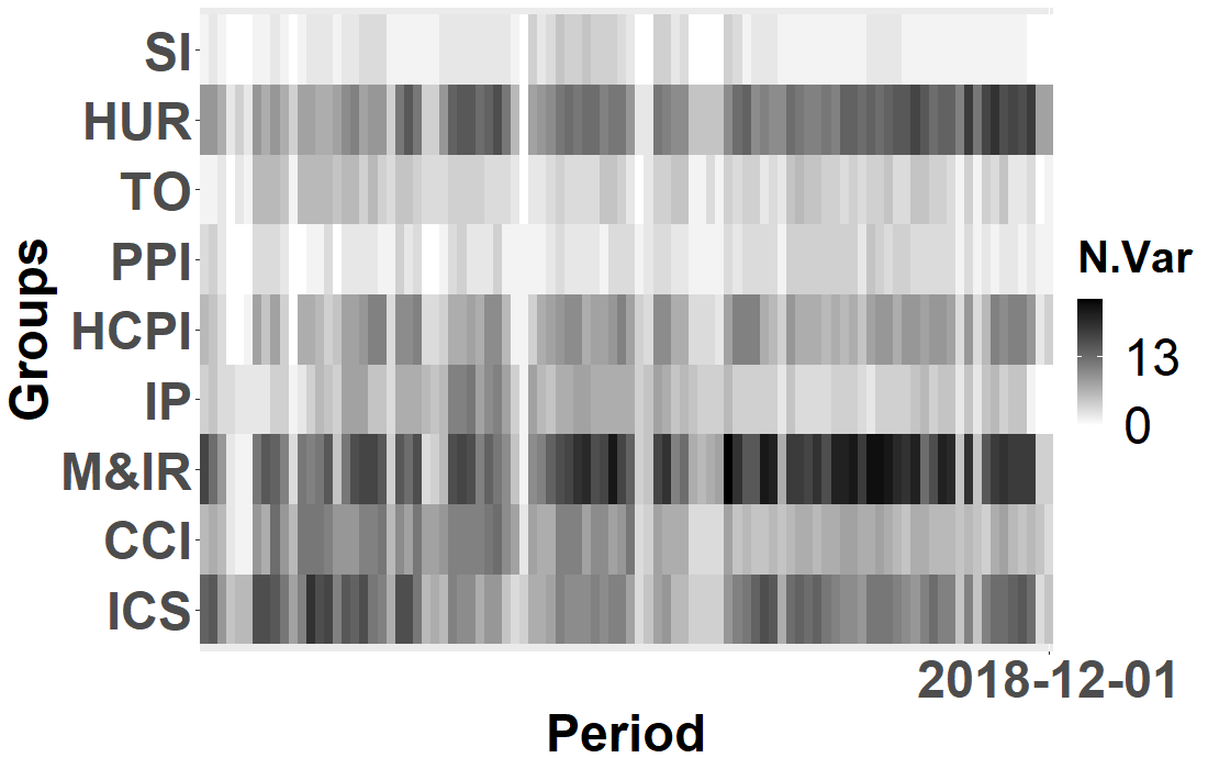
(c)

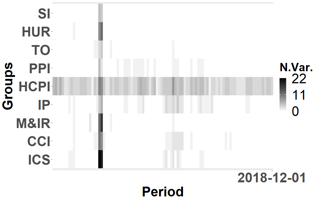
(d)

Figure 2: Heatmaps representing the number of variables selected by LASSO (left) and ARMAr-LAS (right) in the nine main domains. The tuning procedure is BIC.

5 Concluding Remarks

In this paper, we demonstrated that the probability of spurious correlations between stationary orthogonal or weakly correlated processes depends not only on the sample size, but also on the degree of predictors serial correlation. Through this result, we pointed out that serial correlation negatively affects the finite sample estimation and forecasting error bounds of LASSO. In order to improve the performance of LASSO in a time series context, we proposed an approach based on applying LASSO to pre-whitened (i.e., ARMA filtered) time series. This proposal relies on a working model that mitigates large spurious correlation and improves both estimation and forecasting accuracy. We characterized limiting distribution and feature selection consistency, as well as finite sample forecast and estimation error bounds, for our proposal. Furthermore, we assessed its performance through Monte Carlo simulations and an empirical application to Euro Area macroeconomic time series. Through simulations, we observed that ARMAr-LASSO, i.e., LASSO applied to ARMA residuals, reduces the probability of large spurious correlations and outperforms LASSO-based benchmarks from the literature applied to the original predictors in terms of both coefficient estimation and forecasting. The empirical application confirms that ARMAr-LASSO improves the forecasting performance of the benchmarks and produces more parsimonious models.

Supplement - On the Impact of Predictor Serial Correlation on the LASSO

Appendix A Upper Bound for $\psi_{min}$

To support this argument, we start by recalling an inequality that links off-diagonal elements and eigenvalues of $\widehat{\mathbf{C}}_{x}$; namely, $\widehat{\psi}_{min}^{x}\leq 1-\underset{i\neq j}{\text{max}}|\widehat{c}_{ij}^{x}|$ Because of this, for any given $\tau\in[0,1)$ we have

$$\Pr\mathopen{}\mathclose{{}\left(\widehat{\psi}_{min}^{x}\leq 1-\tau}\right)\geq\Pr\mathopen{}\mathclose{{}\left(1-\max_{i\neq j}|\widehat{c}_{ij}^{x}|\leq 1-\tau}\right)\geq\Pr\mathopen{}\mathclose{{}\left(1-|\widehat{c}_{i\neq j}^{x}|\leq 1-\tau}\right)=\Pr\mathopen{}\mathclose{{}\left(|\widehat{c}_{i\neq j}^{x}|\geq\tau}\right)$$

which emphasizes how the probability of a generic sample correlation being large in absolute value affects the probability of the minimum eigenvalue being small – and thus the estimation error bounds of the LASSO, as established by Bickel et al. (2009). As the next example shows, point the inequality $\widehat{\psi}_{min}^{x}\leq 1-\underset{i\neq j}{\text{max}}|\widehat{c}_{ij}^{x}|$ can be easily fixed.

Example A.1:

Let $e_{i}$ and $e_{j}$ be vectors from the standard basis of $\mathbb{R}^{n}$, $i,j\in{1,\dots,N}$. Moreover, let $x_{\pm}=2^{-1/2}(e_{i}\pm e_{j})$, satisfying $||x_{\pm}||_{2}=1$, and let $A$ be a correlation matrix with $a_{k}$ be the $k$-th column. Then we have

$$x_{\pm}^{\prime}Ax_{\pm}=\frac{1}{2}(e_{i}\pm e_{j})^{\prime}(a_{i}\pm a_{j})=\frac{1}{2}(a_{ii}\pm 2a_{ij}+a_{jj})=1\pm a_{ij}\ \ .$$

Thus, $\psi_{min}\leq 1-|a_{ij}|$ for all $i\neq j$ and so

$$\psi_{min}\leq 1-\max_{i\neq j}|a_{ij}|\ \ .$$

Appendix B Theoretical Results

B.1 Proof of Theorem 1

Consider a first order $n$-variate autoregressive process $\mathbf{x}_{t}=\boldsymbol{\phi}^{\prime}\mathbf{x}_{t-1}+\mathbf{u}_{t}$, $t=1,\dots,T$, where $\boldsymbol{\phi}=(\phi_{1},\dots,\phi_{n})^{\prime}$ are the autoregressive coefficients where $|\phi_{i}|<1$ for each $i=1,\dots,n$, and the autoregressive residuals are assumed to be $\mathbf{u}_{t}\sim N\mathopen{}\mathclose{{}\left(\boldsymbol{0}_{n},\boldsymbol{I}_{n}}\right)$. Here $\mathbf{x}_{t}\sim$ $N\mathopen{}\mathclose{{}\left(\boldsymbol{0}_{n},\mathbf{C}_{x}}\right)$ with $\mathopen{}\mathclose{{}\left(\mathbf{C}_{x}}\right)_{ii}=\frac{1}{1-\phi_{i}^{2}}$, and $\mathopen{}\mathclose{{}\left(\mathbf{C}_{x}}\right)_{ij}={c}_{ij}^{x}=0$, for $i\neq j$.

In this setting, we focus on the density of the sample correlation coefficient defined as

$$\widehat{c}_{ij}^{x}=\frac{a_{ij}}{\sqrt{a_{11}}\sqrt{a_{22}}}\ \ ,$$

where $a_{i,j}=\sum_{t=1}^{T}(x_{i,t}-\overline{x}_{i})(x_{j,t}-\overline{x}_{j})=\sum_{t=1}^{T}x_{i,t}x_{j,t}$, since $\overline{x}_{i}=0$, $i\neq j$. In particular, when $c_{ij}^{u}=0$, $b=a_{21}/a_{11}$ and $v=a_{22}-a_{21}^{2}/a_{11}$, then

$$\cfrac{\sqrt{a_{11}}\ b}{\sqrt{v/(T-2)}}=\sqrt{T-2}\cfrac{a_{ij}/\sqrt{a_{11}a_{22}}}{\sqrt{1-a_{ij}^{2}/(a_{11}a_{22})}}=\sqrt{T-2}\cfrac{\widehat{c}_{ij}^{x}}{\sqrt{1-(\widehat{c}_{ij}^{x})^{2}}}\ \ .$$ (7)

Note that $b$ is the least squares regression coefficient of $x_{2t}$ on $x_{1t}$, and $v$ is the sum of the square of residuals of such regression. Thus, to derive the finite sample density of $\widehat{c}_{ij}^{x}$ we need the sample densities of $b$ and $v$.

Remark B.1:

In contrast to asymptotic statements, our theoretical analysis is intended to derive distributions and densities of estimators that hold for $T<\infty$. Hence we will not employ the usual concepts of convergence in probability and in distribution; rather we will use a notion of approximation, whose “precision” needs to be evaluated. The precision of our approximations will be extensively tested under several finite $T$ scenarios in Supplement C.

Sample Distribution of $b$.

We start by deriving the sample distribution of $b$, the OLS regression coefficient for $x_{2}$ on $x_{1}$. The same holds if we regress $x_{1}$ on $x_{2}$.

Lemma B.1:

The sample distribution of $b$ is approximately $N\mathopen{}\mathclose{{}\left(0,\frac{(1-\phi_{1}^{2}\phi_{2}^{2})(1-\phi_{1}^{2})}{(T-1)(1-\phi_{2}^{2})(1-\phi_{1}\phi_{2})^{2}}}\right)$.

Proof: We first focus on the distribution of the sample covariance between $x_{1}$ and $x_{2}$, which is

$$\widehat{Cov}(x_{1},x_{2})=\frac{a_{ij}}{(T-1)}=\\ =\mathopen{}\mathclose{{}\left[\sum_{l=1}^{T-1}\phi_{1}^{l}\widehat{Cov}(u_{1[-l]},u_{2})+\sum_{l=1}^{T-1}\phi_{2}^{l}\widehat{Cov}(u_{2[-l]},u_{1})+\widehat{Cov}(u_{1},u_{2})}\right](1-\phi_{1}\phi_{2})^{-1}\ \ ,$$ (8)

where $\widehat{Cov}(u_{i[-l]},u_{j})=\sum_{t=l+1}^{T}(u_{i,t-l}-\overline{u}_{i})(u_{j,t}-\overline{u}_{j})/(T-l-1)$, for $i\neq j=1,2$, $\overline{u}_{i}=\frac{1}{T-l-1}\sum_{t=l+1}^{T}u_{i,t-l}$ and $\overline{u}_{j}=\frac{1}{T-l-1}\sum_{t=l+1}^{T}u_{j,t}$. Since $u_{1}$ and $u_{2}$ are standard Normal, we have (see Glen et al. 2004 and Supplement H)

$$\widehat{Cov}(u_{1},u_{2})\approx N\mathopen{}\mathclose{{}\left(0\>,\>\cfrac{1}{(T-1)}}\right)\ \ .$$

Moreover, the quantity

$$\eta_{ij}=\sum_{l=1}^{T-1}\phi_{1}^{l}\widehat{Cov}(u_{1[-l]},u_{2})+\sum_{l=1}^{T-1}\phi_{2}^{l}\widehat{Cov}(u_{2[-l]},u_{1})\ \ ,$$

is a linear combination of the sample covariances between the residual of a time series at time $t$ and the lagged residuals of the other time series. Note that $\eta_{ij}$ is a linear combination of $N\mathopen{}\mathclose{{}\left(0,\frac{\phi_{i}^{2l}}{T-l-1}}\right)$, $i=1,2$. However, because $|\phi_{i}|<1$, we can approximate $\eta_{ij}$ as a linear combination of centered Normals with variance $\frac{1}{T-1}$, so that

$$\eta_{ij}\approx N\mathopen{}\mathclose{{}\left(0,\frac{\phi_{1}^{2}+\phi_{2}^{2}-2\phi_{1}^{2}\phi_{2}^{2}}{(T-1)(1-\phi_{1}^{2})(1-\phi_{2}^{2})}}\right)$$

and

$$\widehat{Cov}(x_{1},x_{2})\approx N\mathopen{}\mathclose{{}\left(0\>,\>\frac{1-\phi_{1}^{2}\phi_{2}^{2}}{(T-1)(1-\phi_{1}^{2})(1-\phi_{2}^{2})(1-\phi_{1}\phi_{2})^{2}}}\right)\ \ .$$

Since $a_{11}$ is $T-1$ times the sample variance of $x_{1}$, $a_{11}\approx\frac{T-1}{1-\phi_{1}^{2}}$. Therefore, $b=\frac{a_{21}}{a_{11}}$ is Normally distributed and, based on the approximation of mean and variance of a ratio (see Stuart and Ord 1998), we have $E(b)=0$ and

$$\begin{split}Var(b)=(T-1)^{2}\frac{Var(a_{ij})}{E(a_{11})^{2}}&\approx(T-1)^{2}Var\mathopen{}\mathclose{{}\left(\widehat{Cov}(x_{1},x_{2})}\right)\mathopen{}\mathclose{{}\left(\frac{1-\phi_{1}^{2}}{T-1}}\right)^{2}\\ &=\frac{(1-\phi_{1}^{2}\phi_{2}^{2})(1-\phi_{1}^{2})}{(T-1)(1-\phi_{2}^{2})(1-\phi_{1}\phi_{2})^{2}}\ \ .\end{split}$$

$\blacksquare$

Lemma B.1 shows that the OLS estimate $b$ is normally distributed with a variance that strongly depends on the degree of predictors serial correlation. In this context, it is common to adjust the standard error of the OLS to achieve consistency in the presence of heteroskedasticity and/or serial correlation; this leads, for instance, to the Heteroskedasticity and Autocorrelation Consistent (HAC) estimator of Newey and West (1987) (NW). However, NW estimates can be highly sub-optimal (or inefficient) in the presence of strong serial correlation (Baillie et al., 2024). In Supplement G we provide a simulation study to corroborate the result in Lemma B.1.

Sample Distribution of $v$.

Here we derive the sample distribution of the sum of the square of residuals obtained by regressing $x_{2}$ on $x_{1}$.

Lemma B.2:

The sample distribution of $v$ is approximately $\Gamma\mathopen{}\mathclose{{}\left(\frac{T-2}{2},\frac{2}{1-\phi_{2}^{2}}}\right)$.

Proof: To obtain the sample distribution of $v$ we adapt Theorem 3.3.1 in Anderson (2003, p. 75) to the case of AR(1) processes.

Consider a $(T-1)\times(T-1)$ orthogonal matrix $D=\mathopen{}\mathclose{{}\left(d_{h,t}}\right)$ with first row $\mathbf{x}_{1}^{\prime}/\sqrt{a_{11}}$ and let $s_{h}=\sum_{t=1}^{T-1}d_{h,t}x_{2t}$, $h=1,\dots,(T-1)$, $t=1,\dots,(T-1)$. We have

$$b=\frac{\sum_{t=1}^{T-1}x_{1t}x_{2t}}{\sum_{t=1}^{T-1}x_{1t}^{2}}=\frac{\sum_{t=1}^{T-1}d_{1t}x_{2t}}{\sqrt{a_{11}}}=\frac{s_{1}}{\sqrt{a_{11}}}\ \ .$$

Then, from Lemma 3.3.1 in Anderson (2003, p. 76), we have

$$v=\sum_{t=1}^{T-1}x_{2t}^{2}-b^{2}\sum_{t=1}^{T-1}x_{1t}^{2}=\sum_{t=1}^{T-1}s_{t}^{2}-s_{1}^{2}=\sum_{t=2}^{T-1}s_{t}^{2}\ \ .$$

Thus, $v$ approximates the sum of $T-2$ Normal variables with variance $1/(1-\phi_{2}^{2})$. Now, let $z_{t}$ be the variable obtained by standardizing $x_{2t}$. We have

$$v=\sum_{t=2}^{T-1}s_{t}^{2}\approx\sum_{t=2}^{T-1}\frac{z_{t}^{2}}{1-\phi_{2}^{2}}\ \ .$$ (9)

The right side of (9) is a Gamma distribution with shape parameter $\frac{T-2}{2}$ and rate parameter $\frac{2}{1-\phi_{2}^{2}}$. $\blacksquare$

Sample Density of $\widehat{c}_{ij}^{x}$.

Note that $b$ and $v$ are independent. Using Lemmas B.1 and B.2 and Equation (7) we can now derive the density of the sample distribution of $\widehat{c}_{ij}^{x}$.

Because of Lemma B.1, $\sqrt{a_{11}}b$ is approximately $N\mathopen{}\mathclose{{}\left(0,\frac{1-\phi_{1}^{2}\phi_{2}^{2}}{(1-\phi_{2}^{2})(1-\phi_{1}\phi_{2})^{2}}}\right)$. Let $\delta^{2}=\frac{1-\phi_{1}^{2}\phi_{2}^{2}}{(1-\phi_{2}^{2})(1-\phi_{1}\phi_{2})^{2}}$, $\theta^{2}=\frac{1}{1-\phi_{2}^{2}}$ and $t=\frac{\sqrt{a_{11}}\ b}{\sqrt{v/(T-2)}}$. In the reminder of the proof, we consider the distributions of $b$ and $v$ in Lemmas B.1 and B.2 as exact, not approximate. Thus, we have the densities

$$g\mathopen{}\mathclose{{}\left(\sqrt{a_{11}}b}\right) =\frac{1}{\delta\sqrt{2\pi}}\text{exp}\mathopen{}\mathclose{{}\left(-\frac{a_{11}b^{2}}{2\delta^{2}}}\right)\ ,$$ (10)

$$h(v) =\frac{1}{(2\theta^{2})^{\frac{T-2}{2}}\Gamma\mathopen{}\mathclose{{}\left(\frac{T-2}{2}}\right)}v^{\frac{T-2}{2}-1}\text{exp}\mathopen{}\mathclose{{}\left(-\frac{v}{2\theta^{2}}}\right)\ .$$ (11)

We focus on

$$\begin{split}f(t)&=\int\sqrt{\frac{v}{T-2}}g\mathopen{}\mathclose{{}\left(\sqrt{\frac{v}{T-2}}t}\right)h(v)dv\\ &=\int_{0}^{\infty}\sqrt{\frac{v}{T-2}}\frac{1}{\delta\sqrt{2\pi}}\text{exp}\mathopen{}\mathclose{{}\left(-\frac{vt^{2}}{(T-2)2\delta^{2}}}\right)\frac{v^{\frac{T-2}{2}-1}\text{exp}\mathopen{}\mathclose{{}\left(-\frac{v}{2\theta^{2}}}\right)}{(2\theta^{2})^{\frac{T-2}{2}}\Gamma\mathopen{}\mathclose{{}\left(\frac{T-2}{2}}\right)}dv\\ &=\frac{1}{\sqrt{2\pi(T-2)}\delta(2\theta^{2})^{\frac{T-2}{2}}\Gamma\mathopen{}\mathclose{{}\left(\frac{T-2}{2}}\right)}\int_{0}^{\infty}v^{\frac{1}{2}}v^{\frac{T-2}{2}-1}\text{exp}\mathopen{}\mathclose{{}\left(-\frac{vt^{2}}{(T-2)2\delta^{2}}}\right)\text{exp}\mathopen{}\mathclose{{}\left(-\frac{v}{2\theta^{2}}}\right)dv\\ &=\frac{1}{\sqrt{2\pi(T-2)}\delta(2\theta^{2})^{\frac{T-2}{2}}\Gamma\mathopen{}\mathclose{{}\left(\frac{T-2}{2}}\right)}\int_{0}^{\infty}v^{\frac{T-3}{2}}\text{exp}\mathopen{}\mathclose{{}\left(-\mathopen{}\mathclose{{}\left(\frac{1}{\theta^{2}}\frac{t^{2}}{(T-2)\delta^{2}}}\right)\frac{v}{2}}\right)dv\ .\end{split}$$

Now define $\Upsilon=\frac{1}{\sqrt{2\pi(T-2)}\delta(2\theta^{2})^{\frac{T-2}{2}}\Gamma\mathopen{}\mathclose{{}\left(\frac{T-2}{2}}\right)}$ and $x=\mathopen{}\mathclose{{}\left(\frac{1}{\theta^{2}}+\frac{t^{2}}{(T-2)\delta^{2}}}\right)\frac{v}{2}$. Then

$$\begin{split}f(t)&=\Upsilon\int_{0}^{\infty}\mathopen{}\mathclose{{}\left[2x\mathopen{}\mathclose{{}\left(\frac{1}{\theta^{2}}+\frac{t^{2}}{(T-2)\delta^{2}}}\right)^{-1}}\right]^{\frac{T-3}{2}}\text{exp}\mathopen{}\mathclose{{}\left(-x}\right)dx\\ &=\Upsilon\ 2^{\frac{T-1}{2}}\mathopen{}\mathclose{{}\left(\frac{1}{\theta^{2}}+\frac{t^{2}}{(T-2)\delta^{2}}}\right)^{-\frac{T-1}{2}}\int_{0}^{\infty}x^{\frac{T-1}{2}-1}\text{exp}\mathopen{}\mathclose{{}\left(-x}\right)dx\ .\end{split}$$

The integral on the right hand side can be represented by using the gamma function

$$\Gamma(\alpha)=\int_{0}^{\infty}x^{\alpha-1}\text{exp}\mathopen{}\mathclose{{}\left(-x}\right)dx\ .$$

Thus we obtain

$$\begin{split}f(t)&=\Upsilon\ 2^{\frac{T-1}{2}}\mathopen{}\mathclose{{}\left[\frac{(T-2)\delta^{2}+t^{2}\theta^{2}}{\theta^{2}(T-2)\delta^{2}}}\right]^{-\frac{T-1}{2}}\Gamma\mathopen{}\mathclose{{}\left(\frac{T-1}{2}}\right)\\ &=\frac{\Gamma\mathopen{}\mathclose{{}\left(\frac{T-1}{2}}\right)2^{\frac{T-1}{2}}}{\sqrt{2\pi(T-2)}\delta(2\theta^{2})^{\frac{T-2}{2}}\Gamma\mathopen{}\mathclose{{}\left(\frac{T-2}{2}}\right)}\mathopen{}\mathclose{{}\left[\frac{(T-2)\delta^{2}+t^{2}\theta^{2}}{\theta^{2}(T-2)\delta^{2}}}\right]^{-\frac{T-1}{2}}\\ &=\frac{\Gamma\mathopen{}\mathclose{{}\left(\frac{T-1}{2}}\right)\theta}{\sqrt{\pi(T-2)}\delta\Gamma\mathopen{}\mathclose{{}\left(\frac{T-2}{2}}\right)}\mathopen{}\mathclose{{}\left[\frac{(T-2)\delta^{2}+t^{2}\theta^{2}}{(T-2)\delta^{2}}}\right]^{-\frac{T-1}{2}}.\end{split}$$

Substituting $\delta^{2}$ with $\frac{1-\phi_{1}^{2}\phi_{2}^{2}}{(1-\phi_{2}^{2})(1-\phi_{1}\phi_{2})^{2}}$ and $\theta^{2}$ with $\frac{1}{1-\phi_{2}^{2}}$, we obtain the density

$$\begin{split}f(t)&=\frac{\Gamma\mathopen{}\mathclose{{}\left(\frac{T-1}{2}}\right)(1-\phi_{1}\phi_{2})\sqrt{(1-\phi_{2}^{2}})}{\Gamma\mathopen{}\mathclose{{}\left(\frac{T-2}{2}}\right)\sqrt{\pi(T-2)(1-\phi_{1}^{2}\phi_{2}^{2})(1-\phi_{2}^{2})}}\mathopen{}\mathclose{{}\left[1+\frac{t^{2}(1-\phi_{1}\phi_{2})^{2}(1-\phi_{2}^{2})}{(T-2)(1-\phi_{1}^{2}\phi_{2}^{2})(1-\phi_{2}^{2})}}\right]^{-\frac{T-1}{2}}\\ &=\frac{\Gamma\mathopen{}\mathclose{{}\left(\frac{T-1}{2}}\right)(1-\phi_{1}\phi_{2})}{\Gamma\mathopen{}\mathclose{{}\left(\frac{T-2}{2}}\right)\sqrt{\pi(T-2)(1-\phi_{1}^{2}\phi_{2}^{2})}}\mathopen{}\mathclose{{}\left[1+\frac{t^{2}(1-\phi_{1}\phi_{2})^{2}}{(T-2)(1-\phi_{1}^{2}\phi_{2}^{2})}}\right]^{-\frac{T-1}{2}}\ .\end{split}$$

The density of $w=\widehat{c}_{ij}^{x}\mathopen{}\mathclose{{}\left[1-(\widehat{c}_{ij}^{x})^{2}}\right]^{-\frac{1}{2}}$ is thus

$$\begin{split}f(w)&=\frac{\Gamma\mathopen{}\mathclose{{}\left(\frac{T-1}{2}}\right)(1-\phi_{1}\phi_{2})}{\Gamma\mathopen{}\mathclose{{}\left(\frac{T-2}{2}}\right)\sqrt{\pi(1-\phi_{1}^{2}\phi_{2}^{2})}}\mathopen{}\mathclose{{}\left[1+\frac{w^{2}(1-\phi_{1}\phi_{2})^{2}}{(1-\phi_{1}^{2}\phi_{2}^{2})}}\right]^{-\frac{T-1}{2}}\ .\end{split}$$

Next, define $\kappa(\widehat{c}_{ij}^{x})=w=\widehat{c}_{ij}^{x}\mathopen{}\mathclose{{}\left[1-(\widehat{c}_{ij}^{x})^{2}}\right]^{-\frac{1}{2}}$, from which $\kappa^{\prime}(\widehat{c}_{ij}^{x})=\mathopen{}\mathclose{{}\left[1-(\widehat{c}_{ij}^{x})^{2}}\right]^{-\frac{3}{2}}$, $\ddot{\phi}=\phi_{1}\phi_{2}$ and $\Theta=\mathopen{}\mathclose{{}\left[\Gamma\mathopen{}\mathclose{{}\left(\frac{T-1}{2}}\right)(1-\ddot{\phi})}\right]/\mathopen{}\mathclose{{}\left[\Gamma\mathopen{}\mathclose{{}\left(\frac{T-2}{2}}\right)\sqrt{\pi(1-\ddot{\phi}^{2})}}\right]$. We can use these quantities to write

$$\begin{split}\mathcal{D}_{\widehat{c}_{ij}^{x}}&=f_{w}(\kappa(\widehat{c}_{ij}^{x}))\kappa^{\prime}(\widehat{c}_{ij}^{x})=\Theta\mathopen{}\mathclose{{}\left[1+\mathopen{}\mathclose{{}\left(\widehat{c}_{ij}^{x}(1-(\widehat{c}_{ij}^{x})^{2})^{-\frac{1}{2}}}\right)^{2}\frac{(1-\ddot{\phi})^{2}}{(1-\ddot{\phi}^{2})}}\right]^{-\frac{T-1}{2}}\mathopen{}\mathclose{{}\left[1-(\widehat{c}_{ij}^{x})^{2}}\right]^{-\frac{3}{2}}\\ &=\Theta\mathopen{}\mathclose{{}\left[1+\frac{(\widehat{c}_{ij}^{x})^{2}(1-\ddot{\phi})^{2}}{(1-(\widehat{c}_{ij}^{x})^{2})(1-\ddot{\phi}^{2})}}\right]^{-\frac{T-1}{2}}\mathopen{}\mathclose{{}\left[1-(\widehat{c}_{ij}^{x})^{2}}\right]^{-\frac{3}{2}}\\ &=\Theta\mathopen{}\mathclose{{}\left[\frac{(1-(\widehat{c}_{ij}^{x})^{2})(1-\ddot{\phi}^{2})+(\widehat{c}_{ij}^{x})^{2}(1-\ddot{\phi})^{2}}{(1-(\widehat{c}_{ij}^{x})^{2})(1-\ddot{\phi}^{2})}}\right]^{-\frac{T-1}{2}}\mathopen{}\mathclose{{}\left[1-(\widehat{c}_{ij}^{x})^{2}}\right]^{-\frac{3}{2}}\\ &=\Theta\mathopen{}\mathclose{{}\left[\frac{1-\ddot{\phi}^{2}+2(\widehat{c}_{ij}^{x})^{2}\ddot{\phi}(\ddot{\phi}-1)}{(1-(\widehat{c}_{ij}^{x})^{2})(1-\ddot{\phi}^{2})}}\right]^{-\frac{T-1}{2}}\mathopen{}\mathclose{{}\left[1-(\widehat{c}_{ij}^{x})^{2}}\right]^{-\frac{3}{2}}\\ &=\Theta\mathopen{}\mathclose{{}\left[1-(\widehat{c}_{ij}^{x})^{2}}\right]^{\frac{T-4}{2}}\mathopen{}\mathclose{{}\left[\frac{(1-\ddot{\phi}^{2})}{1-\ddot{\phi}^{2}+2(\widehat{c}_{ij}^{x})^{2}\ddot{\phi}(\ddot{\phi}-1)}}\right]^{\frac{T-1}{2}}\ .\end{split}$$

Thus, the (finite) sample density of $\widehat{c}_{ij}^{x}$, taking the densities in (10) and (11) as exact, is

$$\mathcal{D}_{\widehat{c}_{ij}^{x}}=\frac{\Gamma\mathopen{}\mathclose{{}\left(\frac{T-1}{2}}\right)(1-\ddot{\phi})}{\Gamma\mathopen{}\mathclose{{}\left(\frac{T-2}{2}}\right)\sqrt{\pi}}\mathopen{}\mathclose{{}\left[1-(\widehat{c}_{ij}^{x})^{2}}\right]^{\frac{T-4}{2}}\mathopen{}\mathclose{{}\left(1-\ddot{\phi}^{2}}\right)^{\frac{T-2}{2}}\mathopen{}\mathclose{{}\left[\frac{1}{1-\ddot{\phi}^{2}+2(\widehat{c}_{ij}^{x})^{2}\ddot{\phi}(\ddot{\phi}-1)}}\right]^{\frac{T-1}{2}}\ .$$

$\blacksquare$

B.2 Proof of Theorem 2

Define $V_{T}(\mathbf{a})=\sum_{t=1}^{T}\mathopen{}\mathclose{{}\left[(v_{t}-\mathbf{a}^{\prime}\mathbf{w}_{t}/\sqrt{T})^{2}-v_{t}^{2}}\right]+\lambda\sum_{i=1}^{n+p_{y}}\mathopen{}\mathclose{{}\left[|\beta_{i}^{*}+a_{i}/\sqrt{T}|-|\beta_{i}^{*}|}\right],$ where, $\mathbf{a}=(a_{1}\dots,a_{n+p_{y}})^{\prime}$. We note that $V_{T}(\mathbf{a})$ is minimized at $\sqrt{T}(\widehat{\beta}_{i}-\beta_{i}^{*})$ and

$$V_{T}(\mathbf{a}) =\sum_{t=1}^{T}(v_{t}-\mathbf{a}^{\prime}\mathbf{w}_{t}/\sqrt{T})^{2}+\lambda\sum_{i=1}^{n+p_{y}}|\beta_{i}^{*}+a_{i}/\sqrt{T}|-\mathopen{}\mathclose{{}\left(\sum_{t=1}^{T}v_{t}^{2}+\lambda\sum_{i=1}^{n+p_{y}}|\beta_{i}^{*}|}\right)=$$

$$=\sum_{t=1}^{T}(y_{t}-\mathbf{w}_{t}^{\prime}\boldsymbol{\beta}^{*}-\mathbf{a}^{\prime}\mathbf{w}_{t}/\sqrt{T})^{2}+\lambda\sum_{i=1}^{n+p_{y}}|\beta_{i}^{*}+a_{i}/\sqrt{T}|-\mathopen{}\mathclose{{}\left(\sum_{t=1}^{T}(y_{t}-\mathbf{w}_{t}^{\prime}\boldsymbol{\beta}^{*})^{2}+\lambda\sum_{i=1}^{n+p_{y}}|\beta_{i}^{*}|}\right)$$

$$=A_{T}(\mathbf{a})-A\ \ ,$$

where

$$A_{T}(\mathbf{a})=\sum_{t=1}^{T}(y_{t}-\mathbf{w}_{t}^{\prime}\boldsymbol{\beta}^{*}-\mathbf{a}^{\prime}\mathbf{w}_{t}/\sqrt{T})^{2}+\lambda\sum_{i=1}^{n+p_{y}}|\beta_{i}^{*}+a_{i}/\sqrt{T}|\ \ ,$$

and

$$A=\sum_{t=1}^{T}(y_{t}-\mathbf{w}_{t}^{\prime}\boldsymbol{\beta}^{*})^{2}+\lambda\sum_{i=1}^{n+p_{y}}|\beta_{i}^{*}|\ \ .$$

Since $A$ does not depend on $\mathbf{a}$, minimizing $V_{T}(\mathbf{a})$ with respect to $\mathbf{a}$ is equivalent to minimizing $A_{T}(\mathbf{a})$ with respect to $\mathbf{a}$. Thus, in order to show that $\sqrt{T}(\widehat{\beta}_{i}-\beta_{i}^{*})$ is the minimizer of $V_{T}(\mathbf{a})$ it is sufficient to show that it is the minimizer of $A_{T}(\mathbf{a})$.

$$A_{T}\mathopen{}\mathclose{{}\left(\sqrt{T}(\widehat{\boldsymbol{\beta}}-\boldsymbol{\beta}^{*})}\right) =\sum_{t=1}^{T}\mathopen{}\mathclose{{}\left(y_{t}-(\boldsymbol{\beta}^{*}+\widehat{\boldsymbol{\beta}}-\boldsymbol{\beta}^{*})^{\prime}\mathbf{w}_{t}}\right)^{2}+\lambda\sum_{i=1}^{n+p_{y}}|\beta_{i}^{*}+\widehat{\beta}_{i}-\beta_{i}^{*}|=\noindent$$ (12)

$$=\sum_{t=1}^{T}\mathopen{}\mathclose{{}\left(y_{t}-\widehat{\boldsymbol{\beta}}^{\prime}\mathbf{w}_{t}}\right)^{2}+\lambda\sum_{i=1}^{n+p_{y}}|\widehat{\beta}_{i}|\noindent$$ (13)

$$\leq\sum_{t=1}^{T}\mathopen{}\mathclose{{}\left(y_{t}-(\boldsymbol{\beta}^{*}+\mathbf{a}/\sqrt{T})^{\prime}\mathbf{w}_{t}}\right)^{2}+\lambda\sum_{i=1}^{n+p_{y}}|\beta_{i}^{*}+\mathbf{a}/\sqrt{T}|=A_{T}(\mathbf{a})\noindent$$ (14)

for all $\mathbf{a}$. Thus, we see that

$$\underset{\mathbf{a}\in\mathbb{R}^{n+p_{y}}}{\operatornamewithlimits{argmin\ }}V_{T}(\mathbf{a})=\sqrt{T}(\widehat{\beta}_{i}-\beta_{i}^{*})\ \ .$$

By the Argmin Theorem (Geyer, 1996), we can claim that $\underset{\mathbf{a}\in\mathbb{R}^{n+p_{y}}}{\operatornamewithlimits{argmin\ }}V_{T}(\mathbf{a})\overset{d}{\to}\underset{\mathbf{a}\in\mathbb{R}^{n+p_{y}}}{\operatornamewithlimits{argmin\ }}V(\mathbf{a})$, which implies that $\sqrt{T}(\widehat{\beta}_{i}-\beta_{i}^{*})\overset{d}{\to}\underset{\mathbf{a}\in\mathbb{R}^{n+p_{y}}}{\operatornamewithlimits{argmin\ }}V(\mathbf{a})$, which would prove the Theorem. In what follows we show that $V_{T}(\mathbf{a})\overset{d}{\to}V(\mathbf{a})$ for all $\mathbf{a}$. Note that

$$V_{T}(\mathbf{a})=\sum_{t=1}^{T}\mathopen{}\mathclose{{}\left[(v_{t}-\mathbf{a}^{\prime}\mathbf{w}_{t}/\sqrt{T})^{2}-v_{t}^{2}}\right]+\lambda\sum_{i=1}^{n+p_{y}}\mathopen{}\mathclose{{}\left(|\beta_{i}^{*}+a_{i}/\sqrt{T}|-|\beta_{i}^{*}|}\right)=I(\mathbf{a})+II(\mathbf{a})\ \ .$$

Recall that

$$I(\mathbf{a})=\sum_{t=1}^{T}\mathopen{}\mathclose{{}\left[(v_{t}-\mathbf{a}^{\prime}\mathbf{w}_{t}/\sqrt{T})^{2}-v_{t}^{2}}\right]=\mathbf{a}^{\prime}\mathopen{}\mathclose{{}\left(\frac{1}{T}\sum_{t=1}^{T}\mathbf{w}_{t}\mathbf{w}_{t}^{\prime}}\right)\mathbf{a}-\frac{2}{\sqrt{T}}\sum_{t-1}^{T}v_{t}\mathbf{a}^{\prime}\mathbf{w}_{t}\ \ .$$

As $T\to\infty$ we have $\mathbf{a}^{\prime}\mathopen{}\mathclose{{}\left(\frac{1}{T}\sum_{t=1}^{T}\mathbf{w}_{t}\mathbf{w}_{t}^{\prime}}\right)\mathbf{a}\to\mathbf{a}^{\prime}\boldsymbol{\Sigma}_{w}\mathbf{a}$. Note that $\{v_{t}y_{t-l}\},l\geq 1$, has mean $0$, autocovariance function $\gamma(\cdot)$ such that $\sum_{h=-\infty}^{\infty}|\gamma(h)|<\infty$, and autocorrelation coefficient $\phi_{l}$ such that $\sum_{j=0}^{\infty}\phi_{j}\neq 0$. Thus, we can apply the CLT for dependent processes (see Brockwell and Davis 1991, ch. 7.3) to obtain

$$\frac{1}{\sqrt{T}}\sum_{t=1}^{T}v_{t}\mathbf{a}^{\prime}\mathbf{w}_{t}\overset{d}{\to}N\mathopen{}\mathclose{{}\left(\mathopen{}\mathclose{{}\left(\boldsymbol{0}_{n}^{\prime},\boldsymbol{\mu}_{vy}}\right)^{\prime},\mathbf{a}^{\prime}\mathopen{}\mathclose{{}\left({\begin{array}[]{cc}\sigma_{v}^{2}\mathbf{C}_{u}&\boldsymbol{0}_{n\times p_{y}}\\ \boldsymbol{0}_{p_{y}\times n}&\boldsymbol{\Gamma}_{vy}\\ \end{array}}}\right)\mathbf{a}}\right)\ \ .$$

Therefore, $\frac{1}{\sqrt{T}}\sum_{t=1}^{T}v_{t}\mathbf{a}^{\prime}\mathbf{w}_{t}\overset{d}{\to}\mathbf{a}^{\prime}\mathbf{m},$ where, $\mathbf{m}\sim N\mathopen{}\mathclose{{}\left(\mathopen{}\mathclose{{}\left(\boldsymbol{0}_{n}^{\prime},\boldsymbol{\mu}_{vy}}\right)^{\prime},^{\prime}\mathopen{}\mathclose{{}\left({\begin{array}[]{cc}\sigma_{v}^{2}\mathbf{C}_{u}&\boldsymbol{0}_{n\times p_{y}}\\ \boldsymbol{0}_{p_{y}\times n}&\boldsymbol{\Gamma}_{vy}\\ \end{array}}}\right)}\right)\ \ .$

Applying Slutsky’s theorem, we have $I(\mathbf{a})\overset{d}{\to}\mathbf{a}^{\prime}\mathbf{C}_{w}\mathbf{a}-2\mathbf{a}^{\prime}\mathbf{m}.$

Recall $II(\mathbf{a})=\lambda\sum_{i=1}^{n+p_{y}}\mathopen{}\mathclose{{}\left(|\beta_{i}^{*}+a_{i}/\sqrt{T}|-|\beta_{i}^{*}|}\right)$. When $\beta_{i}^{*}=0$,

$$II(\mathbf{a})=\frac{\lambda}{\sqrt{T}}\sum_{i=1}^{n+p_{y}}|a_{i}|\overset{T\to\infty}{\to}\lambda_{0}\sum_{i=1}^{n+p_{y}}|a_{i}|\ \ ,$$

that is a consequence of the assumption $\lambda/\sqrt{T}\to\lambda_{0}\geq 0$. Thus, when $\beta_{i}^{*}\neq 0$, we have to show that $\lambda\sum_{i=1}^{n+p_{y}}a_{i}Sign(\beta_{i}^{*})I(\beta_{i}^{*}\neq 0)$. Observe that

$$|\beta_{i}^{*}+a_{i}/\sqrt{T}|-|\beta_{i}^{*}|=\frac{1}{\sqrt{T}}\mathopen{}\mathclose{{}\left(|\sqrt{T}\beta_{i}^{*}+a_{i}|-|\sqrt{T}\beta_{i}^{*}|}\right)=$$

$$=\frac{1}{\sqrt{T}}\mathopen{}\mathclose{{}\left(\sqrt{T}Sign(\beta_{i}^{*})\beta_{i}^{*}+Sign(\beta_{i}^{*})a_{i}-|\sqrt{T}\beta_{i}^{*}|}\right)=\frac{1}{\sqrt{T}}Sign(\beta_{i}^{*})a_{i}\ \ ,$$

where the last equality is due to $Sign(\beta_{i})\beta_{i}=|\beta_{i}|$. Therefore

$$\lambda\mathopen{}\mathclose{{}\left(|\beta_{i}^{*}+a_{i}/\sqrt{T}|-|\beta_{i}^{*}|}\right)=\frac{\lambda}{\sqrt{T}}Sign(\beta_{i}^{*})a_{i}\overset{T\to\infty}{\to}\lambda_{0}Sign(\beta_{i}^{*})a_{i}\ \ .$$

We can now say that $\lambda\sum_{i=1}^{n+p_{y}}\mathopen{}\mathclose{{}\left(|\beta_{i}^{*}+a_{i}/\sqrt{T}|-|\beta_{i}^{*}|}\right)\to\lambda_{0}\sum_{i=1}^{n+p_{y}}a_{i}Sign(\beta_{i}^{*})I(\beta_{i}^{*}\neq 0)$. Hence

$$II(\mathbf{a})\to\lambda_{0}\sum_{i=1}^{n+p_{y}}\mathopen{}\mathclose{{}\left[a_{i}Sign(\beta_{i}^{*})I(\beta_{i}^{*}\neq 0)|a_{i}|I(\beta_{i}^{*}=0)}\right]\ \ .$$

Using Slutsky’s theorem, and combining the two results, we have

$$I(\mathbf{a})+II(\mathbf{a})\overset{d}{\to}\mathbf{a}^{\prime}\mathbf{C}_{w}\mathbf{a}-2\mathbf{a}^{\prime}\mathbf{m}+\lambda_{0}\sum_{i=1}^{n+p_{y}}\mathopen{}\mathclose{{}\left[a_{i}Sign(\beta_{i}^{*})I(\beta_{i}^{*}\neq 0)+|a_{i}|I(\beta_{i}^{*}=0)}\right]\ \ ,$$

which shows that $V_{T}(\mathbf{a})\overset{d}{\to}V(\mathbf{a}).$ $\blacksquare$

B.3 Proof of Theorem 3

Define two distinct events:

$$\mathcal{E}.1_{T} =\mathopen{}\mathclose{{}\left\{\mathopen{}\mathclose{{}\left|\widehat{\mathbf{c}}_{i}(11)^{-1}_{i}b_{i}(1)}\right|<\sqrt{T}\mathopen{}\mathclose{{}\left(|\beta_{i}^{*}|-\frac{\lambda}{2T}\mathopen{}\mathclose{{}\left|\widehat{\mathbf{c}}_{i}(11)^{-1}Sign(\beta_{i}^{*})}\right|}\right)}\right\},\ i=1,\dots,s,n+1,\dots,n+s_{y}$$

$$\mathcal{E}.2_{T} =\mathopen{}\mathclose{{}\left\{|b_{i}-b_{i}(2)|\leq\frac{\lambda}{2\sqrt{T}}}\right\},\ i=s+1,\dots,n,n+s_{y}+1,\dots,n+p_{y}\ \ .$$

$\mathcal{E}.1_{T}$ implies that the signs of the relevant predictors are correctly estimated, while $\mathcal{E}.1_{T}$ and $\mathcal{E}.2_{T}$ together imply that the signs of the irrelevant predictors are shrunk to zero. To show $P\mathopen{}\mathclose{{}\left(\exists\lambda\geq 0:Sign(\widehat{\boldsymbol{\beta}})=Sign(\boldsymbol{\beta}^{*})}\right)\rightarrow 1$, it is sufficient to show that $P\mathopen{}\mathclose{{}\left(\exists\lambda\geq 0:Sign(\widehat{\boldsymbol{\beta}})=Sign(\boldsymbol{\beta}^{*})}\right)\geq P\mathopen{}\mathclose{{}\left(\mathcal{E}.1_{T}\cap\mathcal{E}.2_{T}}\right)$. Using the identity of $1-P\mathopen{}\mathclose{{}\left(\mathcal{E}.1_{T}\cap\mathcal{E}.2_{T}}\right)\leq P\mathopen{}\mathclose{{}\left(\mathcal{E}.1_{T}^{C}}\right)+P\mathopen{}\mathclose{{}\left(\mathcal{E}.2_{T}^{C}}\right)$ we have that

$$P\mathopen{}\mathclose{{}\left(\mathcal{E}.1_{T}^{C}}\right)+P\mathopen{}\mathclose{{}\left(\mathcal{E}.2_{T}^{C}}\right)\leq \sum_{i=1}^{s,n+1,\dots,n+s_{y}}P\mathopen{}\mathclose{{}\left(\frac{1}{\sqrt{T}}|\widehat{\mathbf{c}}_{i}(11)^{-1}\mathbf{w}_{i}^{\prime}\mathbf{v}|\geq\sqrt{T}\mathopen{}\mathclose{{}\left(|\beta_{i}^{*}|-\frac{\lambda}{2T}|\widehat{\mathbf{c}}_{i}(11)^{-1}Sign(\beta_{i}^{*})|}\right)}\right)$$

$$+\sum_{i=1}^{s+1,\dots,n,n+s_{y}+1,\dots,n+p_{y}}P\mathopen{}\mathclose{{}\left(\frac{1}{\sqrt{T}}|b_{i}-\mathbf{w}_{i}^{\prime}\mathbf{v}|\geq\frac{\lambda}{2\sqrt{T}}}\right)=I_{T}+II_{T}\ \ .$$

Note that by the union bound, Markov’s inequality and the mixingale concentration inequality (see Hansen 1991, Lemma 2), we have that

$$I_{T} \leq(s+s_{y})P\mathopen{}\mathclose{{}\left(\underset{i}{\operatornamewithlimits{max\ }}\mathopen{}\mathclose{{}\left|\sum_{t=1}^{T}w_{i,t}v_{t}}\right|\geq\widehat{c}_{i}(11)T\mathopen{}\mathclose{{}\left(|\beta_{i}^{*}|-\frac{\lambda}{2T}|\widehat{c}_{i}(11)^{-1}Sign(\beta_{i}^{*})|}\right)}\right)$$

$$\leq\mathopen{}\mathclose{{}\left[\widehat{c}_{i}(11)T\mathopen{}\mathclose{{}\left(|\beta_{i}^{*}|-\frac{\lambda}{2T}|\widehat{c}_{i}(11)^{-1}Sign(\beta_{i}^{*})|}\right)}\right]^{-c_{1}}(s+s_{y})E\mathopen{}\mathclose{{}\left[\max_{l\leq T}\mathopen{}\mathclose{{}\left|\sum_{t=1}^{l}w_{i,t}v_{t}}\right|^{c_{1}}}\right]$$

$$\leq\mathopen{}\mathclose{{}\left[\widehat{c}_{i}(11)T\mathopen{}\mathclose{{}\left(|\beta_{i}^{*}|-\frac{\lambda}{2T}|\widehat{c}_{i}(11)^{-1}Sign(\beta_{i}^{*})|}\right)}\right]^{-c_{1}}(s+s_{y})C_{A}^{c_{1}}\mathopen{}\mathclose{{}\left(\sum_{t=1}^{T}d_{t}^{2}}\right)^{c_{1}/2}\leq$$

$$C(s+s_{y})T^{c_{1}/2}\mathopen{}\mathclose{{}\left[\widehat{c}_{i}(11)T\mathopen{}\mathclose{{}\left(|\beta_{i}^{*}|-\frac{\lambda}{2T}|\widehat{c}_{i}(11)^{-1}Sign(\beta_{i}^{*})|}\right)}\right]^{-c_{1}}$$

$$=C(s+s_{y})\mathopen{}\mathclose{{}\left(\frac{1}{\widehat{c}_{i}(11)\sqrt{T}\mathopen{}\mathclose{{}\left(|\beta_{i}^{*}|-\frac{\lambda}{2T}|\widehat{c}_{i}(11)^{-1}Sign(\beta_{i}^{*})|}\right)}}\right)^{c_{1}}\overset{T\to\infty}{\to}0\ \ .$$ (15)

Conducting a similar analysis for $II_{T}$ we obtain $P\mathopen{}\mathclose{{}\left(\exists\lambda\geq 0:Sign(\widehat{\boldsymbol{\beta}})=Sign(\boldsymbol{\beta}^{*})}\right)\rightarrow 1.$ $\blacksquare$

B.4 Proof of Theorem 4

Before providing the proof of Theorem 4, we introduce some important definitions.

Definition B.1:

Let $\mathopen{}\mathclose{{}\left(\Omega,\mathcal{F},P}\right)$ be a probability space and let $\mathcal{G}$ and $\mathcal{H}$ be sub-$\mathbf{\sigma}$-fields of $\mathcal{F}$. Then

$$\alpha(\mathcal{G},\mathcal{H})=\sup_{G\in\mathcal{G},H\in\mathcal{H}}|\Pr(G\cap H)-\Pr(G)\Pr(H)|$$

is known as the strong mixing coefficient. For a sequence $\mathopen{}\mathclose{{}\left\{X_{t}}\right\}_{-\infty}^{+\infty}$ let $\mathopen{}\mathclose{{}\left\{\mathcal{F}_{-\infty}^{t}}\right\}=\mathbf{\sigma}(\dots,X_{t-1},X_{t})$ and similarly define $\mathopen{}\mathclose{{}\left\{\mathcal{F}_{t+m}^{\infty}}\right\}=\mathbf{\sigma}(X_{t+m},X_{t+m+1},\dots)$. The sequence is said to be $\alpha$-mixing (or strong mixing) if lim${}_{m\rightarrow\infty}\alpha_{m}=0$ where

$$\alpha_{m}=\sup_{t}\alpha(\mathcal{F}_{-\infty}^{t},\mathcal{F}_{t+m}^{\infty}).$$

Definition B.2:

(Mixingale, Davidson (1994), ch. 16). The sequence of pairs $\mathopen{}\mathclose{{}\left\{X_{t},\mathcal{F}}\right\}_{-\infty}^{+\infty}$ in a filtered probability space $\mathopen{}\mathclose{{}\left(\Omega,\mathcal{F},P}\right)$ where the $X_{t}$ are integrable r.v.s is called $L_{p}$-mixingale if, for $p\geq 1$, there exist sequences of non-negative constants $\mathopen{}\mathclose{{}\left\{d_{t}}\right\}_{-\infty}^{+\infty}$ and $\mathopen{}\mathclose{{}\left\{\nu_{m}}\right\}_{0}^{\infty}$ such that $\nu_{m}\rightarrow 0$ as $m\rightarrow\infty$ and

$$||E(X_{t}|\mathcal{F}_{t-m})||_{p}\leq d_{t}\nu_{m}$$

$$||X_{t}-E(X_{t}|\mathcal{F}_{t+m})||_{p}\leq d_{t}\nu_{m+1},$$

hold for all $t$ and $m\geq 0$. Furthermore, we say that $\mathopen{}\mathclose{{}\left\{X_{t}}\right\}$ is $L_{p}$-mixingale of size -$a$ with respect to $\mathcal{F}_{t}$ if $\nu_{m}=O(m^{-a-\epsilon})$ for some $\epsilon>0$.

Definition B.3:

(Near-Epoch Dependence, Davidson (1994), ch. 17). For a possibly vector-valued stochastic sequence $\mathopen{}\mathclose{{}\left\{\mathbf{V}_{t}}\right\}_{-\infty}^{+\infty}$, in a probability space $\mathopen{}\mathclose{{}\left(\Omega,\mathcal{F},P}\right)$ let $\mathcal{F}_{t-m}^{t+m}=\mathbf{\sigma\mathopen{}\mathclose{{}\left(\mathbf{V}_{t-m},\dots,\mathbf{V}_{t+m}}\right)}$, such that $\mathopen{}\mathclose{{}\left\{\mathcal{F}_{t-m}^{t+m}}\right\}_{m=0}^{\infty}$ is a non-decreasing sequence of $\mathbf{\sigma}$-fields. If for $p>0$ a sequence of integrable r.v.s $\mathopen{}\mathclose{{}\left\{X_{t}}\right\}_{-\infty}^{+\infty}$ satisfies

$$||X_{t}-E(X_{t}|{F}_{t-m}^{t+m})||_{p}\leq d_{t}\nu_{m},$$

where $\nu_{m}\rightarrow 0$ and $\mathopen{}\mathclose{{}\left\{d_{t}}\right\}_{-\infty}^{+\infty}$ is a sequence of positive constants, $X_{t}$ will be said to be near-epoch dependent in $L_{p}$-norm ($L_{p}$-NED) on $\mathopen{}\mathclose{{}\left\{\mathbf{V}_{t}}\right\}_{-\infty}^{+\infty}$. Furthermore, we say that $\mathopen{}\mathclose{{}\left\{X_{t}}\right\}$ is $L_{p}$-NED of size -$a$ on $\mathbf{V}_{t}$ if $\nu_{m}=O(m^{-a-\epsilon})$ for some $\epsilon>0$.

Note that we use the same notation for the constants $d_{t}$ and sequence $\nu_{m}$ as for the near-epoch dependence, since they play the same role in both types of dependence.

To simplify the analysis, we frequently make use of arbitrary positive finite constants $C$, as well as of its sub-indexed version $C_{i}$, whose values may change from line to line throughout the paper, but they are always independent of the time and cross-sectional dimension. Generic sequences converging to zero as $T\rightarrow\infty$ are denoted by $\zeta_{T}$. We say a sequence $\zeta_{T}$ is of size $-\phi_{0}$ if $\zeta_{T}=O(T-\phi_{0}-\varepsilon)$ for some $\varepsilon>0$.

Remark B.2:

Under Assumptions 1 and 2 of the main text the process $\{x_{i,t}\}$ is $L_{2b_{1}}$-NED of size $-a$, with $a\geq 1$, while the process $\{q_{i,t}\}$ is $L_{2c_{1}}$-NED of size $-d$, with $d\geq 1$. By Theorems 17.5 in ch.17 of Davidson (1994), they are also $L_{b_{1}}$ and $L_{c_{1}}$-Mixingale, respectively. In later theorems, the NED order and sequence size are important for asymptotic rates. Assumption 5 requires $\mathbf{q}_{t}$ to have slightly more moments than $c_{1}$. More moments mean tighter error bounds and weaker tuning parameter conditions, but a high $c_{2}$ imposes stronger model restrictions. Under strong dependence, fewer moments are needed, and the reduction from $c_{2}$ to $c_{1}$ reflects the cost of allowing greater dependence through a smaller mixing rate.

The proof of Theorem 4 follows that of Theorem 1 in Adamek et al. (2023). We need of the two following auxiliary Lemmas.

Lemma B.3:

Let $\mathcal{B}_{T}\coloneqq\mathopen{}\mathclose{{}\left\{\underset{i\leq n}{\text{max}}\mathopen{}\mathclose{{}\left|\mathopen{}\mathclose{{}\left|\widehat{\boldsymbol{\gamma}}_{i}-\boldsymbol{\gamma}_{i}}\right|}\right|_{\infty}\leq C}\right\}$. Under assumptions 1,2 and 4, for $a\geq 1$ and a sequence $\zeta_{T}\rightarrow 0$ such that $\zeta_{T}\leq\frac{np_{i}}{e}$, if $\sqrt{T}\geq C(np_{i})^{\frac{b_{1}+a-1}{a(b_{1}-1)}}\zeta_{T}^{-\frac{b_{1}+a-1}{a(b_{1}-1)}}$, then $\Pr(\mathcal{B}_{T})\geq 1-3\zeta_{T}\rightarrow 1$.

Proof of Lemma B.3: By the union bound we have

$$\Pr(\mathcal{B}_{T}^{c}) \leq\sum_{i=1}^{n}\sum_{l=1}^{p_{i}}\Pr\mathopen{}\mathclose{{}\left(\mathopen{}\mathclose{{}\left|\sum_{t=1}^{T}(x_{i,t}x_{i,t-l}-E(x_{i,t}x_{i,t-l}))}\right|>CT}\right)$$

$$\leq n\max_{j\leq n}\sum_{l=1}^{p_{j}}P\mathopen{}\mathclose{{}\left(\mathopen{}\mathclose{{}\left|\sum_{t=1}^{T}(x_{j,t}x_{j,t-l}-E(x_{j,t}x_{j,t-l}))}\right|>CT}\right).$$

Now, we apply the Triplex inequality (Jiang, 2009) and obtain

$$P\mathopen{}\mathclose{{}\left(\mathopen{}\mathclose{{}\left|\sum_{t=1}^{T}(x_{j,t}x_{j,t-l}-E(x_{j,t}x_{j,t-l})}\right|>CT}\right)\leq 2m\ \text{exp}\mathopen{}\mathclose{{}\left(\frac{-TC^{2}}{288m^{2}\kappa^{2}}}\right)+$$

$$\cfrac{6}{CT}\sum_{t=1}^{T}E\mathopen{}\mathclose{{}\left[\mathopen{}\mathclose{{}\left|E(x_{j,t}x_{j,t-l}|\mathcal{F}_{t-m})-E(x_{j,t}x_{j,t-l})}\right|}\right]+$$

$$\cfrac{15}{CT}\sum_{t=1}^{T}E\mathopen{}\mathclose{{}\left[\mathopen{}\mathclose{{}\left|x_{j,t}x_{j,t-l}}\right|1_{\{|x_{j,t}x_{j,t-l}|>\kappa\}}}\right]\coloneqq I_{1}+I_{2}+I_{3}\ \ .$$

For the first term we have

$$n\sum_{l=1}^{p_{j}}I_{1}=2np_{i}m\ \text{exp}\mathopen{}\mathclose{{}\left(\frac{-TC^{2}}{288m^{2}\kappa^{2}}}\right),$$

so we need $np_{i}m\ \text{exp}\mathopen{}\mathclose{{}\left(\frac{-T}{m^{2}\kappa^{2}}}\right)\rightarrow 0$.

Without loss of generality, by assumptions 1, 2 and 4, as a consequence of the Cauchy-Schwarz inequality, and Theorems 17.5,17.8-17.10 in Davidson (1994), $\{x_{j,t}x_{j,t-l}-E(x_{j,t}x_{j,t-l})\}$ is $b_{2}$-bounded and $L_{b_{1}}$-mixingale with respect to $\mathcal{F}_{ut}\coloneqq\sigma(\mathbf{u}_{t},\mathbf{u}_{t-1},\dots)$, with non negative mixingale constants $d_{t}\leq C$ and mixingale sequence $\nu_{m}$ of size -$a$, with $a\geq 1$. Therefore, for the Jensen inequality, we have that $E\mathopen{}\mathclose{{}\left(|E(x_{j,t}x_{j,t-l}|\mathcal{F}_{t-m})-E(x_{j,t}x_{j,t-l})|}\right)\leq d_{t}\nu_{m}$. Thus, for the second term we have

$$I_{2}\leq\frac{6}{CT}\sum_{t=1}^{T}d_{t}\nu_{m}\leq C\nu_{m};\ \ \ \ \ n\sum_{l=1}^{p_{j}}I_{2}\leq Cnp_{i}m^{-a},$$

so we need $np_{i}m^{-a}\rightarrow 0$.

For the third term, by Holder’s and Markov’s inequality we have that

$$E\mathopen{}\mathclose{{}\left(|x_{j,t}x_{j,t-l}|1_{|\{x_{j,t}x_{j,t-l}\}|>\kappa}}\right)\leq\mathopen{}\mathclose{{}\left(E\mathopen{}\mathclose{{}\left(|x_{j,t}x_{j,t-l}|^{b_{1}}}\right)}\right)^{1/b_{1}}\mathopen{}\mathclose{{}\left(\frac{E\mathopen{}\mathclose{{}\left(|x_{j,t}x_{j,t-l}|^{b_{1}}}\right)}{\kappa^{b_{1}}}}\right)^{1-1/b_{1}}\leq$$

$$\leq\kappa^{1-b_{1}}E\mathopen{}\mathclose{{}\left(|x_{j,t}x_{j,t-l}|^{b_{1}}}\right),\ \ \ \ \ n\sum_{l=1}^{p_{j}}I_{3}\leq Cnp_{i}\kappa^{1-b_{1}},$$

so we need $np_{i}\kappa^{1-b_{1}}\rightarrow 0.$

We jointly bound the three terms by a sequence $\zeta_{T}\rightarrow 0$ as follows:

$$Cnp_{i}m\ \text{exp}\mathopen{}\mathclose{{}\left(\frac{-T}{m^{2}\kappa^{2}}}\right)\leq\zeta_{T},\ \ \ \ \ Cnp_{i}m^{-a}\leq\zeta_{T},\ \ \ \ \ Cnp_{i}\kappa^{1-b_{1}}\leq\zeta_{T}.$$

First, note that $m\in\mathbb{Z}^{+},\ \kappa>0$. Moreover, we assume that $\frac{\zeta_{T}}{np_{i}}\leq\frac{1}{e}\Longrightarrow\frac{\zeta_{T}}{np_{i}m}\leq\frac{1}{e}$. We isolate $\kappa$ from the first and third terms

$$Cnp_{i}m\ \text{exp}\mathopen{}\mathclose{{}\left(\frac{-T}{m^{2}\kappa^{2}}}\right)\leq\zeta_{T}\ \ \Longleftrightarrow\ \ \kappa\leq C\frac{\sqrt{T}}{m}\frac{1}{\text{log}\mathopen{}\mathclose{{}\left(np_{i}m/\zeta_{T}}\right)}\ \ ,$$

$$Cnp_{i}\kappa^{1-b_{1}}\leq\zeta_{T}\ \ \Longleftrightarrow\ \ \kappa\geq C(np_{i})^{1/(b_{1}-1)}\zeta_{T}^{-1/(b_{1}-1)}\ \ .$$

Since we have a lower and upper bound on $\kappa$, we need to make sure both bounds are satisfied:

$$C_{1}(np_{i})^{1/(b_{1}-1)}\zeta_{T}^{-1/(b_{1}-1)}\leq C_{1}\frac{\sqrt{T}}{m}\frac{1}{\sqrt{\text{log}\mathopen{}\mathclose{{}\left(np_{i}m/\zeta_{T}}\right)}}$$

$$\Longleftrightarrow m\sqrt{\text{log}\mathopen{}\mathclose{{}\left(np_{i}m/\zeta_{T}}\right)}\leq C\sqrt{T}(np_{i})^{-1/(b_{1}-1)}\zeta_{T}^{1/(b_{1}-1)}\ \ .$$

Isolating $m$, we have that $Cnp_{i}m^{-a}\leq\zeta_{T}\Longleftrightarrow m\geq C(np_{i})^{1/a}\zeta_{T}^{-1/a}.$ Assuming $\frac{\zeta_{T}}{np_{i}m}\leq\frac{1}{e}$, we have that $m\leq m\sqrt{\text{log}(np_{i}m/\zeta_{T})}$ and therefore we need to ensure that

$$C(np_{i})^{1/a}\zeta_{T}^{-1/a}\leq C\sqrt{T}(np_{i})^{-1/(b_{1}-1)}\zeta_{T}^{1/(b_{1}-1)}$$

$$\Longleftrightarrow\sqrt{T}\geq C(np_{i})^{\frac{b_{1}+a-1}{a(b_{1}-1)}}\zeta_{T}^{-\frac{b_{1}+a-1}{a(b_{1}-1)}}\ \ .$$ (16)

Thus, when (16) is satisfied, $n\sum_{l=1}^{p_{j}}I_{1}+I_{2}+I_{3}\leq 3\zeta_{T}$ and $\Pr(\mathcal{B}_{T})\geq 1-3\zeta_{T}$. $\blacksquare$

Note that under assumption 4 we have that $\Pr(\mathcal{B}_{T})\geq 1-2\zeta_{T}$, since $Cnp_{i}m^{-a}=0$, instead of $1-3\zeta_{T}$, given that $\{x_{j,t}x_{j,t-l}\}$ is a $L_{m_{1}}$-mixingale of size $-\infty$.

Lemma B.4:

Let $\mathcal{A}_{T}\coloneqq\mathopen{}\mathclose{{}\left\{\underset{i\leq n+p_{y},t\leq T}{\text{max}}\mathopen{}\mathclose{{}\left|\sum_{t=1}^{T}w_{i,t}v_{t}}\right|\leq\frac{T\lambda}{4}}\right\}$. Under assumption 1, 2 and 5, for $\zeta_{T}$ as in Lemma B.3, if $\lambda\geq\frac{C(n+p_{y})^{1/c_{1}}\zeta_{T}^{-1/c_{1}}}{\sqrt{T}}$, then $\Pr(\mathcal{A}_{T})\geq 1-\zeta_{T}$.

Proof of Lemma B.4: By assumptions 1, 2, 5 and Theorems 17.5, 17.9 and 17.10 in Davidson (1994), we have that $\{w_{i,t}v_{i,t}\}$ is an $L_{m}$-mixingale of appropriate size. By the union bound, the Markov’s inequality and the Hansen’s mixingale concentration inequality, it follows that

$$P\mathopen{}\mathclose{{}\left(\max_{i\leq n+p_{y},l\leq T}\mathopen{}\mathclose{{}\left[\mathopen{}\mathclose{{}\left|\sum_{t=1}^{l}w_{i,t}v_{t}}\right|}\right]>\frac{T\lambda}{4}}\right)\leq\sum_{i=1}^{n+p_{y}}P\mathopen{}\mathclose{{}\left(\max_{l\leq T}\mathopen{}\mathclose{{}\left[\mathopen{}\mathclose{{}\left|\sum_{t=1}^{l}w_{i,t}v_{t}}\right|}\right]>\frac{T\lambda}{4}}\right)\leq$$

$$\mathopen{}\mathclose{{}\left(\frac{T\lambda}{4}}\right)^{-c_{1}}\sum_{i=1}^{n+p_{y}}E\mathopen{}\mathclose{{}\left[\max_{l\leq T}\mathopen{}\mathclose{{}\left|\sum_{t=1}^{l}w_{i,t}v_{t}}\right|^{c_{1}}}\right]\leq\mathopen{}\mathclose{{}\left(\frac{T\lambda}{4}}\right)^{-c_{1}}\sum_{i=1}^{n+p_{y}}C_{1}^{c_{1}}\mathopen{}\mathclose{{}\left(\sum_{t=1}^{T}d_{t}^{2}}\right)^{c_{1}/2}\leq$$

$$C(n+p_{y})T^{c_{1}/2}\mathopen{}\mathclose{{}\left(\frac{T\lambda}{4}}\right)^{-c_{1}}\ \ .$$

This means that $\Pr(\mathcal{A}_{T})\geq 1-C\mathopen{}\mathclose{{}\left(n+p_{y}}\right)\mathopen{}\mathclose{{}\left(\frac{1}{\sqrt{T}\lambda}}\right)^{c_{1}}$. The Lemma follows from choosing $(n+p_{y})(\lambda\sqrt{T})^{-c_{1}}\leq\zeta_{T}$, for which $\lambda\geq\frac{C(n+p_{y})^{1/c_{1}}\zeta_{T}^{-1/c_{1}}}{\sqrt{T}}$. $\blacksquare$

Proof of Theorem 4: We combine the results of Lemmas B.3 and B.4. By Lemma B.4 we have $\Pr(\mathcal{A}_{T})\geq 1-\zeta_{T}$ when $\lambda\geq C\zeta_{T}^{-1/c_{1}}\frac{(n+p_{y})^{1/c_{1}}}{\sqrt{T}}$. For Lemma B.3 we need $\zeta_{T}\leq\frac{np_{i}}{e}$, $\sqrt{T}\geq C(np_{i})^{\frac{b_{1}+a-1}{a(b_{1}-1)}}\zeta_{T}^{-\frac{b_{1}+a-1}{a(b_{1}-1)}}$. Therefore, for $n$ and $T$ sufficiently large, we have $\Pr(\mathcal{B}_{T})\geq 1-\zeta_{T}$. The result then follows by the union bound $\Pr(\mathcal{A}_{T}\cap\mathcal{B}_{T})\geq 1-C\zeta_{T}\rightarrow 1$ as $n,T\rightarrow\infty$. The result of the Theorem follows by choosing $\zeta_{T}=\mathopen{}\mathclose{{}\left(\sqrt{\text{log(T)}}}\right)^{-1}$. $\blacksquare$

B.5 Proof Theorem 5

The proof is based on the relevant contribution on LASSO oracle inequalities provided in Chapter 6 of Bühlmann and van de Geer (2011).

By Lemma 6.1 in Bühlmann and van de Geer (2011) we obtain

$$\frac{1}{T}\mathopen{}\mathclose{{}\left|\mathopen{}\mathclose{{}\left|\mathbf{W}^{\prime}(\widehat{\boldsymbol{\beta}}-\boldsymbol{\beta}^{*})}\right|}\right|_{2}^{2}\leq\frac{2}{T}\mathbf{W}\mathbf{v}\bigl{(}\widehat{\boldsymbol{\beta}}-\boldsymbol{\beta}^{*}\bigl{)}+\lambda\Bigl{(}||\boldsymbol{\beta}^{*}||_{1}-||\widehat{\boldsymbol{\beta}}||_{1}\Bigl{)}.$$

Note that the empirical process $\frac{2}{T}\mathbf{W}\mathbf{v}(\widehat{\boldsymbol{\beta}}-\boldsymbol{\beta}^{*})$, i.e., the random part can be easily bounded in terms of the $\ell_{1}$ norm of the parameters, such that,

$$\frac{1}{T}\mathopen{}\mathclose{{}\left|\mathbf{W}^{\prime}(\widehat{\boldsymbol{\beta}}-\boldsymbol{\beta}^{*})}\right|\leq\frac{2}{T}\mathopen{}\mathclose{{}\left|\mathopen{}\mathclose{{}\left|\mathbf{W}\mathbf{v}}\right|}\right|_{\infty}||\widehat{\boldsymbol{\beta}}-\boldsymbol{\beta}^{*}||_{1}.$$

The penalty $\lambda$ is chosen such that $T^{-1}\mathopen{}\mathclose{{}\left|\mathopen{}\mathclose{{}\left|\mathbf{W}\mathbf{v}}\right|}\right|_{\infty}\leq\lambda$. The event $\mathcal{A}_{T}\coloneqq\mathopen{}\mathclose{{}\left\{T^{-1}\mathopen{}\mathclose{{}\left|\mathopen{}\mathclose{{}\left|\mathbf{W}\mathbf{v}}\right|}\right|_{\infty}\leq\frac{\lambda_{0}}{2}}\right\}$ has to hold with high probability, where $\lambda_{0}\leq\frac{\lambda}{2}$. Lemma B.4 and Theorem 4 of the main text prove that $\Pr(\mathcal{A}_{T})\geq 1-\zeta_{T}$ and $\Pr(\mathcal{A}_{T}\cap\mathcal{B}_{T})\geq 1-C\zeta_{T}$ for some $C>0$.

Since $\lambda\geq 2\lambda_{0}$ under $\mathcal{A}_{T}$ and by Assumption 6, we can use the following dual norm inequality (Theorem 6.1 Bühlmann and van de Geer 2011)

$$\frac{1}{T}|\mathopen{}\mathclose{{}\left|\mathopen{}\mathclose{{}\left|\mathbf{W}^{\prime}(\widehat{\boldsymbol{\beta}}-\boldsymbol{\beta}^{*})}\right|}\right|_{2}^{2}+\lambda\mathopen{}\mathclose{{}\left|\mathopen{}\mathclose{{}\left|\widehat{\boldsymbol{\beta}}-\boldsymbol{\beta}^{*}}\right|}\right|_{1}\leq\frac{4\tilde{s}\lambda}{\gamma_{w}^{2}},$$

which leads to

$$\frac{1}{T}\mathopen{}\mathclose{{}\left|\mathopen{}\mathclose{{}\left|\mathbf{W}^{\prime}(\widehat{\boldsymbol{\beta}}-\boldsymbol{\beta}^{*})}\right|}\right|_{2}^{2}\leq\frac{4\tilde{s}\lambda^{2}}{\gamma_{w}^{2}},$$

$$\mathopen{}\mathclose{{}\left|\mathopen{}\mathclose{{}\left|\widehat{\boldsymbol{\beta}}-\boldsymbol{\beta}^{*}}\right|}\right|_{1}\leq\frac{4\tilde{s}\lambda}{\gamma_{w}^{2}},$$

with probability at least $1-\zeta_{t}$. The result of the Theorem follows from choosing $\zeta_{t}=C\mathopen{}\mathclose{{}\left(\sqrt{\text{log}(T)}}\right)^{-1}$, for a large enough constant $C>0$. $\blacksquare$

Appendix C Monte Carlo Experiments

In this Section, we conduct Monte Carlo experiments to assess numerically the approximation of the density of $\widehat{c}_{ij}^{x}$ described in Section 2.1. After, we expand the theoretical results in more generic contexts, relaxing the assumption that the predictors are orthogonal Gaussian AR(1) processes. We indicate the density of $\widehat{c}_{ij}^{x}$ obtained by simulations as $d_{s}(\widehat{c}_{ij}^{x})$.

C.1 Numerical Approximation of $d_{s}(\widehat{c}_{12}^{x})$ to $\mathcal{D}_{\widehat{c}_{12}^{x}}$

We generate data from the bivariate process $\mathbf{x}_{t}=\mathbf{D}_{\phi}\mathbf{x}_{t-1}+\mathbf{u}_{t}$ for $t=1,\dots,T$, where $\mathbf{D}_{\phi}$ is a $2\times 2$ diagonal matrix with the same autocorrelation coefficient $\phi$ in both positions along the diagonal, and $u_{t}\sim N(\boldsymbol{0}_{2},\boldsymbol{I}_{2})$. We consider $T=50,100,250$ and $\phi=0.3,0.6,0.9,0.95$ – thus, the parameter $\ddot{\phi}$ in $\mathcal{D}_{\widehat{c}_{12}^{x}}$, here equal to $\phi^{2}$, takes values 0.09, 0.36, 0.81, 0.90. The first row of Figure 3 (Plots (a), (b), (c)) shows, for various values of $T$ and $\ddot{\phi}$, the density $d_{s}(\widehat{c}_{12}^{x})$ generated through 5000 Monte Carlo replications. The second row of Figure 3 (Plots (d), (e), (f)) shows the corresponding $\mathcal{D}_{\widehat{c}_{12}^{x}}$. These were plotted using 5000 values of the argument starting at -1 and increasing by steps of size 0.0004 until 1. As expected, we observe that the degree of approximation of $d_{s}(\widehat{c}_{12}^{x})$ to $\mathcal{D}_{\widehat{c}_{12}^{x}}$ improves as $T$ increases and/or $\ddot{\phi}$ decreases. In particular, Plots (a) and (d) in Figure 3, where $T=50$, show that $\mathcal{D}_{\widehat{c}_{12}^{x}}$ approximates $d_{s}(\widehat{c}_{12}^{x})$ well for a low-to-intermediate degree of serial correlation ($\ddot{\phi}\leq 0.36$, i.e. $\phi\leq 0.6$). In contrast, in cases with high degree of serial correlation ($\ddot{\phi}\geq 0.81$, i.e. $\phi\geq 0.9$), $\mathcal{D}_{\widehat{c}_{12}^{x}}$ has larger tails compared to $d_{s}(\widehat{c}_{12}^{x})$; that is, the latter over-estimates the probability of large spurious correlations. However, it is noteworthy that the difference between the two densities is negligible for $T\geq 100$ (Figure 3, Plots (b) and (e) for $T=100$, and Plots (c) and (f) for $T=250$), also with high degree of serial correlation ($\ddot{\phi}\approx 0.90$, i.e. $\phi=0.95$). These numerical experiments corroborate the fact that the sample cross-correlation between orthogonal Gaussian AR(1) processes is affected by the degree of serial correlation in a way that is well approximated by $\mathcal{D}_{\widehat{c}_{12}^{x}}$. In fact, for a sufficiently large finite $T$, we observe that $\Pr\mathopen{}\mathclose{{}\left\{|\widehat{c}_{12}^{x}|\geq\tau}\right\}$, $\tau>0$, increases with $\ddot{\phi}$ in a similar way for $d_{s}(\widehat{c}_{12}^{x})$ and $\mathcal{D}_{\widehat{c}_{12}^{x}}$.

(a)

(b)

(c)

(d)

(e)

(f)

Figure 3: Monte Carlo densities for $\widehat{c}_{12}^{x}$ (top) and corresponding $\mathcal{D}_{\widehat{c}_{12}^{x}}$ (bottom) for various $T$ and $\ddot{\phi}$.

The Impact of $Sign(\ddot{\phi})$

In Section 2.1 of the main text we pointed out that the impact of $\ddot{\phi}$ on $\mathcal{D}_{\widehat{c}_{12}^{x}}$ depends on $Sign(\ddot{\phi})$. In particular, when $-1<\ddot{\phi}<0$, an increment on $|\ddot{\phi}|$ makes the density of $\widehat{c}_{12}^{x}$ more concentrated around $0$. In order to validate this result, we run simulations with $T=100$ and different values for the second element of the diagonal of $\mathbf{D}_{\phi}$; namely, $-0.3,-0.6,-0.9,-0.95$. Results are shown in Plots (a) and (b) of Figure 4. In this case, we see that when $Sign(\phi_{1})\neq Sign(\phi_{2})$ and $|\ddot{\phi}|$ increases, $d_{s}(\widehat{c}_{12}^{x})$ increases its concentration around $0$ in a way that is, again, well approximated by $\mathcal{D}_{\widehat{c}_{12}^{x}}$.

C.2 General Case

To generalize our findings to the case of non-Gaussian weakly correlated AR and ARMA processes, we generate predictors according to the following DGPs: ${x}_{1t}=(\phi+0.1){x}_{1t-1}+(\phi+0.1){x}_{1t-2}-0.2{x}_{1t-3}+u_{1t}$, and ${x}_{2t}=\phi x_{2t-1}+\phi x_{2t-2}+{u}_{2t}+0.8{u}_{2t-1}$, where $t=1,\ldots,100$ and $\phi=0.15,0.3,0.45,0.475$. Moreover, we generate $u_{1t}$ and $u_{2t}$ from a bivariate Laplace distribution with means $0$, variances $1$, and $c_{12}^{u}=0.2$. In these more general cases, we do not know an approximate theoretical density for $\widehat{c}_{12}^{u}$. Therefore, we rely entirely on simulations to show the effect of serial correlation on $\Pr\mathopen{}\mathclose{{}\left\{|\widehat{c}_{12}^{x}|\geq\tau}\right\}$. Plot (c) of Figure 4 shows $d_{s}(\widehat{c}_{12}^{x})$ obtained from 5000 Monte Carlo replications for the different values of $\phi$. In short, also in the more general cases where predictors are non-Gaussian, weakly correlated AR(3) and ARMA(2,1) processes, the probability of getting large sample cross-correlations depends on the degree of serial correlation. More simulation results are provided below.

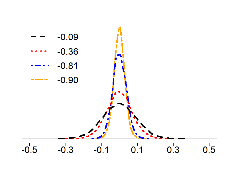
(a)

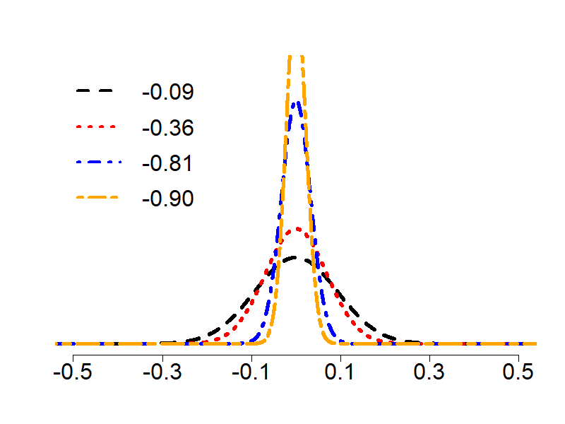
(b)

(c)

Figure 4: Monte Carlo densities for $\widehat{c}_{12}^{x}$ (a) and corresponding $\mathcal{D}_{\widehat{c}_{12}^{x}}$ (b), for $T$=100 and various (negative) $\ddot{\phi}$’s. Monte Carlo densities for $\widehat{c}_{12}^{x}$ in the case of Laplace weakly correlated AR(3) and ARMA(2,1) processes, for $T=100$ and various $\phi$’s (c).

C.3 More General Cases

We study the density of $\widehat{c}_{12}^{x}$ in three different cases: non-Gaussian processes; weakly and high cross-correlated processes; and ARMA processes with different order. Note that for the first two cases the variables are AR(1) processes with $T=100$ and autocorrelation coefficient $\phi=0.3,0.6,0.9,0.95$. Since we do not have $\mathcal{D}_{\widehat{c}_{12}^{x}}$ for these cases, we rely on the densities obtained on 5000 Monte Carlo replications, i.e. $d_{s}(\widehat{c}_{12}^{x})$, to show the effect of serial correlation on $\Pr\mathopen{}\mathclose{{}\left\{|\widehat{c}_{12}^{x}|\geq\tau}\right\}$.

The Impact of non-Gaussianity

The theoretical contribution reported in Section 2.1 requires the Gaussianity of $u_{1}$ and $u_{2}$. With the following simulation experiments we show that the impact of $\ddot{\phi}$ on the density of $\widehat{c}_{12}^{x}$ is relevant also when $u_{1t}$ and $u_{2t}$ are non-Gaussian random variables. To this end, we generate $u_{1t}$ and $u_{2t}$ from the following distributions: Laplace with mean 0 and variance 1 (case (a)); Cauchy with location parameter 0 and scale parameter 1 (case (b)); and from a $t$-student with 1 degree of freedom (case (c)). Figure 5 reports the results of the simulation experiment. We can state that regardless the distribution of the processes, whenever $Sign(\phi_{1})=Sign(\phi_{2})$, the probability of large values of $\widehat{c}_{12}^{x}$ increases with $\ddot{\phi}$. As a curiosity, this result is more evident for the case of Laplace variables, whereas for Cauchy and $t$-student the effect of $\ddot{\phi}$ declines.

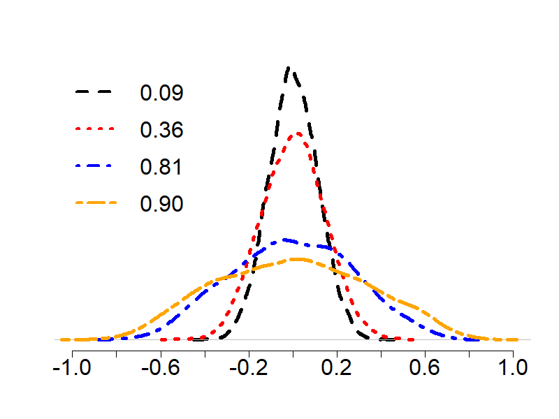
(a)

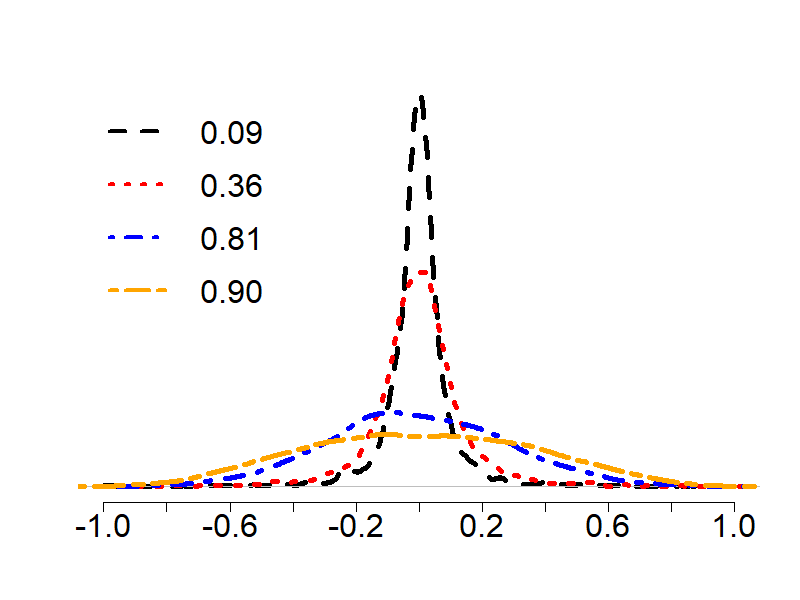
(b)

(c)

Figure 5: Simulated density of $\widehat{c}_{12}^{x}$ in the case of non-Gaussian processes, for $T=100$ and various values of $\phi$.

The Impact of Population Cross-Correlation

Since orthogonality is an unrealistic assumption for most economic applications, here we admit population cross-correlation. In Figure 6 we report $d_{s}(\widehat{c}_{12}^{x})$ when the processes are weakly cross-correlated with $c_{12}^{u}=0.2$, and when the processes are multicollinear with $c_{12}^{u}=0.8$ (usually we refer to multicollinearity when $c_{12}^{u}\geq 0.7$). We observe that the impact of $\ddot{\phi}$ on $d_{s}(\widehat{c}_{12}^{x})$ depends on the degree of (population) cross-correlation as follows. In the case of weakly correlated processes, an increase in $\ddot{\phi}$ yields a high probability of observing large sample correlations in absolute value. In the case of multicollinear processes, on the other hand, an increase in $\ddot{\phi}$ leads to a high probability of underestimating the true population cross-correlation.

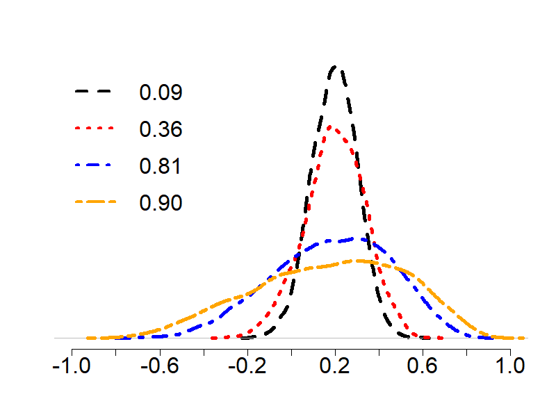
(a)

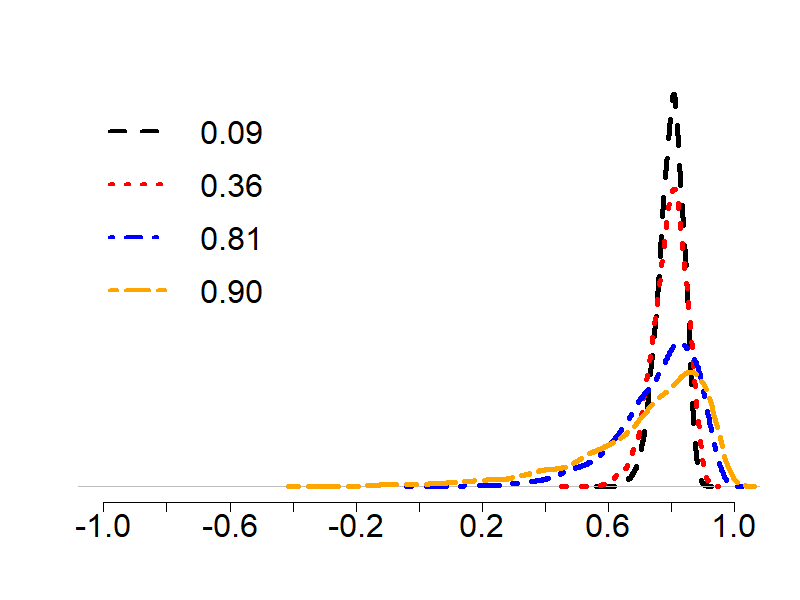
(b)

Figure 6: $d_{s}(\widehat{c}_{12}^{x})$ obtained through simulations in the case of $c_{12}^{x}=0.2$ (a) and $c_{12}^{x}=0.8$ (b), for $T=100$ and various values of $\phi$.

Density of $\widehat{c}_{12}^{x}$ in the case of ARMA$(p_{i},q_{i})$ processes

To show the effect of serial correlation on a more general case, we generate $x_{1}$ and $x_{2}$ through the following ARMA processes

$${x}_{1t}={\phi}{x}_{1t-1}+\phi{x}_{1t-2}-\phi{x}_{1t-3}{u}_{1t}+0.5u_{1t-1},$$

$${x}_{2t}={\phi}{x}_{2t-1}+\phi{x}_{2t-2}+{u}_{2t}+0.7{u}_{2t-1}-0.4u_{3t-2},$$

where $t=1,\dots,100$ and $u_{i}\sim N(0,1)$. In Figure 7 we report the density of $\widehat{c}_{12}^{x}$ in the case of $T=100$ and $\phi=0.1,0.2,0.3,0.33$. With no loss of generality we can observe that $d_{s}(\widehat{c}_{12}^{x})$ gets larger as $\phi$ increases, that is $\Pr\mathopen{}\mathclose{{}\left\{|\widehat{c}_{12}^{x}|\geq\tau}\right\}$ increases with $|\phi|$.

Figure 7: Densities of $d_{s}(\widehat{c}_{12}^{x})$ between two uncorrelated ARMA Gaussian processes, for $T=100$ and various values of $\phi$.

Appendix D Least Square Applied to Working Model

Here, we describe two asymptotic results on estimation and forecasting performance of the non-penalized fit, which we prove under strong simplifying assumptions and validate in more general settings through simulations in Section 4. The following Proposition describes the asymptotic behavior of the non-penalized, least square fit of working model (4) in terms of estimation.

Proposition D.1:

Let $\phi_{x}=\frac{E(x_{i,t}x_{i,t-1})}{E(x_{i,t}^{2})}$, for each $i=1,\dots,n$. Moreover, let $\sigma_{y}^{2}$ be the variance of $y$ and $R^{2}={\boldsymbol{\alpha}^{*}}^{\prime}\mathbf{C}_{x}\boldsymbol{\alpha}^{*}/\sigma_{y}^{2}$ be the asymptotic coefficient of determination, where $\mathbf{X}\mathbf{X}^{\prime}/T\ \overset{p}{\to}\ \mathbf{C}_{x}$. As $T\to\infty$, the least squares estimates for model (4) converge as follows: $\widehat{\phi}_{y}\ \overset{p}{\to}\ \phi_{x}R^{2}+\phi_{\varepsilon}(1-R^{2}),\ \ \ \widehat{\boldsymbol{\alpha}}\ \overset{p}{\to}\ \boldsymbol{\alpha}^{*}$.

Proof: To simplify notation, we report results in matrix form, where the subscript $-j$ denotes the corresponding matrix or vector of $j$ period lagged values. We start with the case of common AR(1) restriction. We consider the following model $\mathbf{y}=\mathbf{X}_{-1}^{\prime}\boldsymbol{\alpha}^{*}+\boldsymbol{\varepsilon},\ \mathbf{X}=\phi\mathbf{X}_{-1}+\mathbf{U},\ \boldsymbol{\varepsilon}=\phi_{\varepsilon}\boldsymbol{\varepsilon}_{-1}+\boldsymbol{\omega}$. As a consequence of Assumption 2 in the text of the main paper:

$$\mathbf{X}_{-1}\boldsymbol{\varepsilon}/T\ \overset{p}{\to}\ 0;\ \ \ \ \ \phi\mathbf{X}_{-1}\mathbf{U}^{\prime}/T\ \overset{p}{\to}\ 0;\ \ \ \ \ \phi_{\varepsilon}\boldsymbol{\varepsilon}_{-1}^{\prime}\boldsymbol{\omega}/T\ \overset{p}{\to}\ 0;\ \ \ \ \ \mathbf{U}_{-1}\boldsymbol{\omega}/T\ \overset{p}{\to}\ 0.$$

Let:

$$\mathbf{X}_{-1}\mathbf{X}_{-1}^{\prime}/T\ \overset{p}{\to}\ \mathbf{C}_{x};\ \ \ \ \ \boldsymbol{\varepsilon}^{\prime}\boldsymbol{\varepsilon}/T\ \overset{p}{\to}\ c_{\varepsilon}.$$

Moreover, $var(y)=\sigma_{y}^{2}={\boldsymbol{\alpha}^{*}}^{\prime}\mathbf{C}_{x}\boldsymbol{\alpha}^{*}+c_{\varepsilon}$.

Our working model consists in using $(\mathbf{U}_{-1}^{\prime},\mathbf{y}_{-1})^{\prime}$ as regressors of the OLS model to obtain $\widehat{\boldsymbol{\alpha}}$ and $\widehat{\phi}_{y}$. We have the following preliminary results:

$$\mathbf{U}_{-1}\mathbf{U}_{-1}^{\prime}/T\ \overset{p}{\to}\ \mathbf{C}_{u};\ \ \ \ \ \mathbf{U}_{-1}\mathbf{y}/T\ \overset{p}{\to}\ \mathbf{C}_{u}\boldsymbol{\alpha}^{*};\ \ \ \ \ \mathbf{U}_{-1}\mathbf{y}_{-1}/T\ \overset{p}{\to}\ 0;\ \ \ \ \ \mathbf{y}_{-1}^{\prime}\mathbf{y}/T\ \overset{p}{\to}\ \phi{\boldsymbol{\alpha}^{*}}^{\prime}\mathbf{C}_{x}\boldsymbol{\alpha}^{*}+\phi_{\varepsilon}c_{\varepsilon}.$$

Thus,

$$\begin{bmatrix}\widehat{\phi}_{y}\\ \widehat{\boldsymbol{\alpha}}\end{bmatrix}=\begin{bmatrix}\mathbf{y}_{-1}^{\prime}\mathbf{y}_{-1}/T&\mathbf{y}_{-1}^{\prime}\mathbf{U}_{-1}^{\prime}/T\\ \mathbf{U}_{-1}\mathbf{y}_{-1}/T&\mathbf{U}_{-1}\mathbf{U}_{-1}^{\prime}/T\end{bmatrix}^{-1}\begin{bmatrix}\mathbf{y}_{-1}^{\prime}\mathbf{y}/T\\ \mathbf{U}_{-1}\mathbf{y}/T\end{bmatrix},$$

and applying the preliminary results above gives:

$$\begin{bmatrix}\widehat{\phi}_{y}\\ \widehat{\boldsymbol{\alpha}}\end{bmatrix}\ \overset{p}{\to}\ \begin{bmatrix}\sigma_{y}^{2}&0\\ 0&\mathbf{C}_{u}\end{bmatrix}^{-1}\begin{bmatrix}\phi{\boldsymbol{\alpha}^{*}}^{\prime}\mathbf{C}_{x}\boldsymbol{\alpha}^{*}+\phi_{\varepsilon}c_{\varepsilon}\\ \mathbf{C}_{u}\boldsymbol{\alpha}^{*}\end{bmatrix},$$

from which

$$\begin{bmatrix}\widehat{\phi}_{y}\\ \widehat{\boldsymbol{\alpha}}\end{bmatrix}\ \overset{p}{\to}\ \cfrac{1}{\sigma_{y}^{2}}\begin{bmatrix}1&0\\ 0&\cfrac{\sigma_{y}^{2}}{\mathbf{C}_{u}}\end{bmatrix}\begin{bmatrix}\phi{\boldsymbol{\alpha}^{*}}^{\prime}\mathbf{C}_{x}\boldsymbol{\alpha}^{*}+\phi_{\varepsilon}c_{\varepsilon}\\ \mathbf{C}_{u}\boldsymbol{\alpha}^{*}\end{bmatrix}.$$

After some algebra we get:

$$\widehat{\phi}_{y}\ \overset{p}{\to}\ \phi R^{2}+\phi_{\varepsilon}(1-R^{2})\ ,\ \ \ \ \ \ \ \ \ \widehat{\boldsymbol{\alpha}}\ \overset{p}{\to}\ \boldsymbol{\alpha}^{*}.$$

The results holds for $\phi=\phi_{x}$. Note that in the case of a common AR(1) restriction with a common factor, the proof follows by considering the same procedure where $\phi_{x}R^{2}=\mathopen{}\mathclose{{}\left(\phi_{f}\Delta_{f}+\phi\Delta_{z}}\right)R^{2}$, where $\Delta_{f}$ and $\Delta_{z}$ are the fraction of variance of $X$ explained by $f$ (the common factor) and $z$ (the idiosyncratic component), respectively.

$\blacksquare$

D.1 Monte Carlo Experiments: ARMAr-OLS

In this section, we validate the theoretical properties of our working model within an asymptotic, non-sparse context, by estimating it with the OLS. We refer to it as ARMAr-OLS. We set $T=1000$, $n=10$ and $\alpha_{i}^{*}=1$ for $i=1,\dots,10$. We then conduct a comparative analysis between OLS applied to $x$’s and ARMAr-OLS. We first simulate $x_{i,t}=f_{t}+z_{i,t}$, where $f_{t}=\phi f_{t-1}+\delta_{t},$ $z_{i,t}=\phi z_{i,t-1}+\eta_{i,t},$ $\varepsilon_{t}=\phi\varepsilon_{t-1}+\omega_{t},$ where $\delta_{t}\sim i.i.d.\ N(0,1)$, $\eta_{i,t}\sim i.i.d.\ N(0,1)$ with $\mathopen{}\mathclose{{}\left(\mathbf{C}_{\eta}}\right){ij}=c_{ij}^{\eta}=\rho^{|i-j|}$, and $\omega_{t}\sim i.i.d.\ N(0,\sigma_{\omega}^{2})$. We investigate different situations with $\phi=0.3,0.6,0.9,0.95$. Table 6 presents the average on 1000 simulations of root mean square forecast error (RMSFE) and coefficient estimation error (CoEr) of ARMAr-OLS relative to OLS for various values of $\phi$ under the common AR(1) restriction when $\lambda=0$ and when $\lambda\neq 0$. We observe an improvement in RMSFE for ARMAr-OLS over OLS as $\phi\rightarrow 1^{-}$, due to the SNR in ARMAr-OLS, which also results in more accurate coefficient estimates. To generalize these results, we conduct a new simulation study where $f_{t}=0.9f_{t-1}+\delta_{t}$; ${z}_{i,t}=0.8{z}_{i,t-1}+{\eta}_{i,t},\ i=1,2,3$; ${z}_{j,t}=0.6{z}_{j,t-1}+0.3{z}_{j,t-2}+{\eta}_{j,t},\ j=4,5,6$; ${z}_{wt}=0.5{z}_{wt-1}+0.4{z}_{wt-2}+{\eta}_{wt}+0.3{\eta}_{wt-1},\ w=7,8$; ${z}_{kt}=0.7{z}_{kt-1}+{\eta}_{kt}+0.4{\eta}_{kt-1},\ k=9,10$, for $t=1,\dots,T$. The error term follows an AR(2) pattern, $\varepsilon_{t}=0.7\varepsilon_{t-1}+0.2\varepsilon_{t-2}+\omega_{t}$. The results are now reported in Table 7 and show that, also in a general setting out-off the common AR(1) restriction, our working model maintains an advantage in both coefficient estimation and forecasting compared to the classical OLS applied to the $x$’s.

Table 6: Root mean square forecast error (RMSFE) and coefficient estimation error (CoEr) of ARMAr-OLS relative to OLS for various values of $\phi$ for $\lambda=0$ and $\lambda\neq 0$, under common AR(1) restriction.

	$\lambda=0$					$\lambda\neq 0$
$\phi$	0.3	0.6	0.9	0.95		0.3	0.6	0.9	0.95
RMSFE	0.96	0.79	0.44	0.32		0.95	0.79	0.46	0.31
CoEr	0.93	0.74	0.36	0.26		0.94	0.72	0.35	0.25

Table 7: Root mean square forecast error (RMSFE) and coefficient estimation error (CoEr) of ARMAr-OLS relative to OLS for $\lambda=0$ and $\lambda\neq 0$, under general AR/ARMA setting

	$\lambda=0$	$\lambda\neq 0$
RMSFE	0.60	0.57
CoEr	0.14	0.29

Appendix E Experiments

Table 8: DGPs (A).

			n			50					150					300
			$\phi$		0.3	0.6	0.9	0.95		0.3	0.6	0.9	0.95		0.3	0.6	0.9	0.95
SNR
	RMSFE
		LASSOy			0.98	0.88	0.73	0.74		0.99	0.89	0.80	0.80		0.99	0.89	0.83	0.83
		FaSel			0.96	0.97	0.95	0.95		0.97	0.96	0.96	0.95		0.88	0.92	0.95	0.94
		ARMAr-LAS			0.98	0.83	0.62	0.62		0.98	0.86	0.72	0.70		0.99	0.84	0.75	0.72
	% TP
		LASSO			46.70	43.70	55.10	57.40		43.20	39.80	46.10	47.80		40.30	37.40	44.50	45.20
0.5		LASSOy			47.50	44.20	36.90	38.60		44.10	40.10	34.70	37.80		40.70	38.20	33.50	35.70
		FaSel			7.90	11.40	42.10	44.00		18.30	25.10	39.40	44.80		39.20	36.00	41.70	45.40
		ARMAr-LAS			49.90	51.80	54.60	58.10		45.90	47.80	51.00	54.80		42.50	45.10	48.00	52.20
	% FP
		LASSO			2.20	7.00	42.60	45.40		0.70	3.00	17.90	17.40		0.40	1.80	10.00	9.60
		LASSOy			2.40	4.00	11.10	16.10		0.70	1.40	5.20	7.20		0.40	0.80	3.20	4.20
		FaSel			1.20	5.00	37.10	38.80		0.70	2.90	16.20	17.20		11.60	9.30	9.90	9.60
		ARMAr-LAS			2.70	2.90	3.30	3.10		0.80	1.00	1.10	1.00		0.50	0.50	0.50	0.50
	RMSFE
		LASSOy			0.98	0.90	0.79	0.80		0.99	0.89	0.90	0.83		0.99	0.92	0.89	0.89
		FaSel			0.97	0.97	0.94	0.94		0.97	0.98	0.97	0.93		0.89	0.94	0.93	0.95
		ARMAr-LAS			0.97	0.83	0.62	0.63		0.96	0.82	0.73	0.67		0.99	0.84	0.76	0.73
	% TP
		LASSO			61.10	56.70	60.90	62.90		58.80	54.00	56.60	57.20		57.20	52.50	54.90	56.80
1		LASSOy			61.70	57.10	51.70	52.50		59.00	54.10	49.60	51.80		57.40	52.40	48.60	52.00
		FaSel			12.60	16.60	44.50	49.10		29.60	37.20	49.60	54.80		51.20	48.40	52.50	57.40
		ARMAr-LAS			64.70	65.60	68.10	71.10		61.50	62.20	65.10	68.00		59.60	60.00	62.80	67.40
	% FP
		LASSO			2.70	7.70	42.00	44.40		1.00	3.40	17.40	16.30		0.40	2.00	9.60	9.40
		LASSOy			2.80	5.00	19.50	24.20		1.00	1.80	8.10	9.50		0.40	1.00	4.70	6.00
		FaSel			2.20	6.20	36.90	39.70		0.80	3.60	16.30	16.60		11.50	7.30	9.30	9.30
		ARMAr-LAS			3.20	3.60	3.80	3.90		1.10	1.10	1.20	1.30		0.50	0.50	0.60	0.60
	RMSFE
		LASSOy			1.00	0.97	0.92	0.94		1.00	0.97	0.98	0.94		1.00	0.98	0.96	0.97
		FaSel			0.99	1.01	0.95	0.97		0.96	0.99	0.94	0.89		0.92	0.95	0.93	0.95
		ARMAr-LAS			0.98	0.85	0.64	0.63		0.98	0.83	0.71	0.67		0.98	0.85	0.73	0.74
	% TP
		LASSO			90.70	84.60	80.50	82.60		89.80	84.00	80.60	81.40		88.90	83.20	81.90	81.60
5		LASSOy			90.70	85.20	79.40	81.30		89.80	84.10	79.90	80.90		89.00	83.50	81.10	81.00
		FaSel			27.50	34.10	58.50	64.30		57.30	65.80	77.00	81.90		81.10	79.20	81.30	83.90
		ARMAr-LAS			92.70	92.40	93.60	94.70		91.10	91.30	92.70	94.10		90.50	90.70	92.10	93.70
	% FP
		LASSO			3.80	9.70	41.00	42.90		1.30	4.00	15.00	12.90		0.60	2.40	8.60	7.80
		LASSOy			3.70	8.30	34.60	37.30		1.30	3.40	12.60	11.20		0.60	2.10	7.60	7.00
		FaSel			7.00	13.10	38.90	40.90		2.30	5.50	15.80	15.00		6.90	5.90	8.60	8.40
		ARMAr-LAS			4.50	4.40	4.40	4.80		1.40	1.40	1.50	1.50		0.70	0.70	0.70	0.80
	RMSFE
		LASSOy			1.00	0.98	0.96	0.95		1.00	0.98	0.97	0.95		1.00	0.99	0.99	0.99
		FaSel			1.01	0.95	0.95	0.95		1.02	0.98	0.92	0.89		0.92	0.94	0.91	0.90
		ARMAr-LAS			0.97	0.80	0.63	0.62		0.97	0.84	0.70	0.63		0.99	0.84	0.74	0.68
	% TP
		LASSO			97.60	94.20	89.40	90.60		97.40	93.20	90.20	88.80		97.20	93.60	91.20	90.00
10		LASSOy			97.60	94.40	89.30	90.60		97.40	93.40	89.80	88.20		97.20	93.60	90.60	89.50
		FaSel			35.50	45.60	65.70	72.30		67.10	77.50	88.60	90.60		90.00	90.10	90.90	92.60
		ARMAr-LAS			98.30	98.40	98.50	98.80		98.10	98.00	98.20	98.70		97.70	97.80	98.10	98.60
	% FP
		LASSO			4.00	10.00	39.70	42.20		1.30	4.20	13.40	11.40		0.70	2.60	8.00	7.00
		LASSOy			4.00	9.20	37.20	40.30		1.30	3.80	12.40	10.40		0.70	2.50	7.40	6.30
		FaSel			10.70	19.00	40.20	41.90		3.10	6.80	15.50	14.20		6.80	5.80	8.40	7.90
		ARMAr-LAS			4.40	4.60	4.80	4.90		1.60	1.50	1.60	1.60		0.80	0.80	0.80	0.80

Table 9: DGPs (B).

			n			50					150					300
			$\phi$		0.3	0.6	0.9	0.95		0.3	0.6	0.9	0.95		0.3	0.6	0.9	0.95
SNR
	RMSFE
		LASSOy			0.99	0.89	0.75	0.73		0.98	0.88	0.82	0.84		0.99	0.91	0.85	0.87
		FaSel			0.99	1.01	1.00	0.98		0.98	1.00	0.98	0.98		1.21	1.03	0.98	0.97
		ARMAr-LAS			0.97	0.82	0.65	0.60		1.00	0.84	0.74	0.75		1.00	0.86	0.76	0.76
	% TP
		LASSO			39.30	34.70	50.40	53.10		25.20	22.60	32.90	32.80		19.50	17.40	23.80	24.60
		LASSOy			40.40	36.00	28.00	31.70		25.70	23.80	19.00	21.00		20.20	18.20	13.50	16.10
0.5		FaSel			2.00	8.40	46.10	48.80		1.40	5.40	29.50	31.70		58.50	41.80	22.20	23.50
		ARMAr-LAS			43.60	45.40	47.80	52.60		28.00	31.80	35.20	39.40		21.10	24.30	26.40	31.60
	% FP
		LASSO			9.70	12.90	42.60	45.30		4.20	6.10	19.00	18.40		2.80	4.00	10.60	10.00
		LASSOy			9.90	11.20	14.50	19.30		4.30	5.40	7.20	8.40		3.00	3.20	4.20	4.80
		FaSel			0.40	4.20	41.80	44.90		0.20	1.80	19.40	19.70		49.30	34.00	11.60	11.20
		ARMAr-LAS			11.00	12.10	12.20	13.30		4.70	5.60	6.00	6.20		3.70	3.40	3.50	3.70
	RMSFE
		LASSOy			0.98	0.89	0.79	0.81		0.99	0.91	0.91	0.85		1.00	0.91	0.85	0.87
		FaSel			1.00	1.00	1.00	0.98		0.99	1.02	0.99	0.95		1.21	1.04	0.96	0.95
		ARMAr-LAS			0.96	0.81	0.62	0.63		0.97	0.85	0.79	0.69		0.98	0.84	0.76	0.73
	% TP
		LASSO			58.60	50.40	57.20	60.90		44.70	38.50	41.90	42.60		37.60	31.50	34.80	35.60
		LASSOy			59.00	51.80	42.40	46.80		45.30	39.80	31.90	34.80		38.00	31.90	26.30	29.40
1		FaSel			4.40	13.00	50.80	55.00		3.70	10.00	37.40	41.00		63.10	48.20	32.30	34.60
		ARMAr-LAS			62.10	63.30	65.40	69.20		48.60	50.30	53.50	57.80		40.30	42.40	46.50	52.30
	% FP
		LASSO			12.50	15.40	42.60	44.70		6.00	7.90	18.80	17.70		3.70	4.80	10.40	9.90
		LASSOy			12.70	14.30	22.40	26.20		6.10	6.90	10.20	10.90		3.70	4.10	6.00	6.50
		FaSel			0.60	5.10	42.60	44.00		0.20	2.00	19.80	20.40		48.80	34.00	11.60	11.20
		ARMAr-LAS			14.00	14.30	14.60	14.90		6.70	7.10	7.10	7.50		4.00	4.30	4.50	4.60
	RMSFE
		LASSOy			1.00	0.97	0.93	0.94		1.00	0.98	0.96	0.95		1.00	0.97	0.95	0.97
		FaSel			1.07	1.05	0.97	0.98		1.06	1.07	0.96	0.90		1.23	1.02	0.96	0.91
		ARMAr-LAS			0.97	0.84	0.67	0.64		0.97	0.85	0.73	0.66		0.97	0.86	0.74	0.71
	% TP
		LASSO			93.30	86.50	81.60	83.70		89.50	80.90	73.80	73.00		85.70	76.40	71.80	68.90
		LASSOy			93.30	87.00	80.30	82.00		89.40	81.40	72.60	71.50		85.70	76.80	70.00	67.10
5		FaSel			53.90	61.40	73.50	76.50		51.80	55.90	71.70	75.90		82.70	73.70	71.80	71.10
		ARMAr-LAS			94.70	95.30	95.60	96.50		91.20	90.90	92.10	94.30		88.20	87.50	90.50	91.60
	% FP
		LASSO			16.50	20.10	42.90	46.50		8.40	10.90	16.70	14.40		5.40	6.80	9.90	8.40
		LASSOy			16.30	18.90	37.80	41.90		8.30	10.30	14.80	12.90		5.40	6.40	8.80	7.60
		FaSel			5.90	16.40	45.30	48.80		1.60	6.30	21.40	21.20		40.40	26.30	13.40	12.20
		ARMAr-LAS			17.20	17.00	17.20	17.80		8.80	8.80	9.00	9.00		5.70	5.60	5.80	5.80
	RMSFE
		LASSOy			1.00	0.99	0.96	0.95		1.00	0.99	0.97	0.97		1.00	0.99	0.98	0.97
		FaSel			1.06	1.03	0.98	0.97		1.05	1.05	0.93	0.85		1.12	1.04	0.91	0.87
		ARMAr-LAS			0.97	0.82	0.67	0.63		0.98	0.84	0.71	0.64		0.98	0.87	0.74	0.67
	% TP
		LASSO			98.90	96.50	92.20	93.40		97.80	93.70	87.70	85.30		96.40	91.70	85.30	81.90
		LASSOy			98.90	96.60	91.60	92.90		97.80	93.90	87.00	84.50		96.50	91.80	85.20	81.30
10		FaSel			89.60	85.80	86.60	88.90		86.60	84.00	88.40	88.80		91.10	88.10	86.50	86.70
		ARMAr-LAS			99.20	99.40	99.40	99.60		98.50	98.50	98.70	99.20		97.60	97.70	98.20	98.10
	% FP
		LASSO			16.90	21.60	44.30	46.60		8.80	11.20	15.60	12.90		5.50	7.20	9.20	7.80
		LASSOy			16.70	21.00	41.70	44.50		8.70	11.00	14.70	12.10		5.40	7.00	8.70	7.30
		FaSel			12.20	23.40	48.30	50.90		3.30	10.10	23.20	21.90		26.90	20.30	13.60	12.70
		ARMAr-LAS			17.70	17.30	17.80	17.30		9.30	9.10	9.30	9.10		5.80	6.00	5.90	5.90

Appendix F List of Time Series in the Euro Area Data

We report the list of series for the Euro Area dataset adopted in the forecasting exercise (obtained from Proietti and Giovannelli (2021)). As for the FRED data, the column tcode denotes the data transformation for a given series $x_{t}$: (1) no transformation; (2) $\Delta x_{t}$; (3)$\Delta^{2}x_{t}$; (4) $\text{log}(x_{t})$; (5) $\Delta\text{log}(x_{t})$; (6) $\Delta^{2}\text{log}(x_{t})$. (7) $\Delta(x_{t}/x_{t-}-1.0)$.

The acronyms for the sectors refer to:

• ICS: Industry & Construction Survey

• CCI: Consumer Confidence Indicators

• M&IR: Money & Interest Rates

• IP: Industrial Production

• HCPI: Harm. Consumer Price Index

• PPI: Producer Price Index

• TO: Turnover & Retail Sale

• HUR: Harm. Unemployment rate

• SI: Service Svy.

Table 10: A sample long table.

ID	Description	Area	Sector	Tcode
1	Ind Svy: Employment Expectations	EA	ICS	1
2	Ind Svy: Export Order-Book Levels	EA	ICS	1
3	Ind Svy: Order-Book Levels	EA	ICS	1
4	Ind Svy: Mfg - Selling Price Expectations	EA	ICS	1
5	Ind Svy: Production Expectations	EA	ICS	1
6	Ind Svy: Production Trend	EA	ICS	1
7	Ind Svy: Mfg - Stocks Of Finished Products	EA	ICS	1
8	Constr. Svy: Price Expectations	EA	ICS	1
9	Ind Svy: Export Order Book Position	EA	ICS	1
10	Ind Svy: Production Trends In Recent Mth.	EA	ICS	1
11	Ind Svy: Selling Prc. Expect. Mth. Ahead	EA	ICS	1
12	Ret. Svy: Employment	EA	ICS	1
13	Ret. Svy: Orders Placed With Suppliers	EA	ICS	1
14	Constr. Svy: Synthetic Bus. Indicator	FR	ICS	1
15	Bus. Svy: Constr. Sector - Capacity Utilisation Rate	FR	ICS	1
16	Constr. Svy: Activity Expectations	FR	ICS	1
17	Constr. Svy: Price Expectations	FR	ICS	1
18	Constr. Svy: Unable To Increase Capacity	FR	ICS	1
19	Constr. Svy: Workforce Changes	FR	ICS	1
20	Constr. Svy: Workforce Forecast Changes	FR	ICS	1
21	Svy: Mfg Output - Order Book & Demand	FR	ICS	1
22	Svy: Mfg Output - Order Book & Foreign Demand	FR	ICS	1
23	Svy: Mfg Output - Personal Outlook	FR	ICS	1
24	Svy: Auto Ind - Order Book & Demand	FR	ICS	1
25	Svy: Auto Ind - Personal Outlook	FR	ICS	1
26	Svy: Basic & Fab Met Pdt Ex Mach & Eq - Personal Outlook	FR	ICS	1
27	Svy: Ele & Elec Eq, Mach Eq - Order Book & Demand	FR	ICS	1
28	Svy: Ele & Elec Eq, Mach Eq - Order Book & Foreign Demand	FR	ICS	1
29	Svy: Ele & Elec Eq, Mach Eq - Personal Outlook	FR	ICS	1
30	Svy: Mfg Output - Price Outlook	FR	ICS	1
31	Svy: Mfg Of Chemicals & Chemical Pdt - Order Book & Demand	FR	ICS	1
32	Svy: Mfg Of Chemicals & Chemical Pdt - Personal Outlook	FR	ICS	1
33	Svy: Mfg Of Food Pr & Beverages - Order Book & Demand	FR	ICS	1
34	Svy: Mfg Of Food Pr & Beverages - Order Book & Foreign Demand	FR	ICS	1
35	Svy: Mfg Of Trsp Eq - Finished Goods Inventories	FR	ICS	1
36	Svy: Mfg Of Trsp Eq - Order Book & Demand	FR	ICS	1
37	Svy: Mfg Of Trsp Eq - Order Book & Foreign Demand	FR	ICS	1
38	Svy: Mfg Of Trsp Eq - Personal Outlook	FR	ICS	1
39	Svy: Oth Mfg, Mach & Eq Rpr & Instal - Ord Book & Demand	FR	ICS	1
40	Svy: Oth Mfg, Mach & Eq Rpr & Instal - Ord Book & Fgn Demand	FR	ICS	1
41	Svy: Oth Mfg, Mach & Eq Rpr & Instal - Personal Outlook	FR	ICS	1
42	Svy: Other Mfg - Order Book & Demand	FR	ICS	1
43	Svy: Rubber, Plastic & Non Met Pdt - Order Book & Demand	FR	ICS	1
44	Svy: Rubber, Plastic & Non Met Pdt - Order Book & Fgn Demand	FR	ICS	1
45	Svy: Rubber, Plastic & Non Met Pdt - Personal Outlook	FR	ICS	1
46	Svy: Total Ind - Order Book & Demand	FR	ICS	1
47	Svy: Total Ind - Order Book & Foreign Demand	FR	ICS	1
48	Svy: Total Ind - Personal Outlook	FR	ICS	1
49	Svy: Total Ind - Price Outlook	FR	ICS	1
50	Svy: Wood & Paper, Print & Media - Ord Book & Fgn Demand	FR	ICS	1
51	Trd. & Ind: Bus Sit	DE	ICS	1
52	Trd. & Ind: Bus Expect In 6Mo	DE	ICS	1
53	Trd. & Ind: Bus Sit	DE	ICS	1
54	Trd. & Ind: Bus Climate	DE	ICS	1
55	Cnstr Ind: Bus Climate	DE	ICS	1
56	Mfg: Bus Climate	DE	ICS	1
57	Mfg: Bus Climate	DE	ICS	1
58	Mfg Cons Gds: Bus Climate	DE	ICS	1
59	Mfg (Excl Fbt): Bus Climate	DE	ICS	1
60	Whsle (Incl Mv): Bus Climate	DE	ICS	1
61	Mfg: Bus Sit	DE	ICS	1
62	Mfg: Bus Sit	DE	ICS	1
63	Mfg (Excl Fbt): Bus Sit	DE	ICS	1
64	Mfg (Excl Fbt): Bus Sit	DE	ICS	1
65	Cnstr Ind: Bus Expect In 6Mo	DE	ICS	1
66	Cnstr Ind: Bus Expect In 6Mo	DE	ICS	1
67	Mfg: Bus Expect In 6Mo	DE	ICS	1
68	Mfg: Bus Expect In 6Mo	DE	ICS	1
69	Mfg Cons Gds: Bus Expect In 6Mo	DE	ICS	1
70	Mfg (Excl Fbt): Bus Expect In 6Mo	DE	ICS	1
71	Mfg (Excl Fbt): Bus Expect In 6Mo	DE	ICS	1
72	Rt (Incl Mv): Bus Expect In 6Mo	DE	ICS	1
73	Whsle (Incl Mv): Bus Expect In 6Mo	DE	ICS	1
74	Bus. Conf. Indicator	IT	ICS	1
75	Order Book Level: Ind	ES	ICS	1
76	Order Book Level: Foreign - Ind	ES	ICS	1
77	Order Book Level: Investment Goods	ES	ICS	1
78	Order Book Level: Int. Goods	ES	ICS	1
79	Production Level - Ind	ES	ICS	1
80	Cons. Confidence Indicator	EA	CCI	1
81	Cons. Svy: Economic Situation Last 12 Mth. - Emu 11/12	EA	CCI	1
82	Cons. Svy: Possible Savings Opinion	FR	CCI	1
83	Cons. Svy: Future Financial Situation	FR	CCI	1
84	Svy - Households, Economic Situation Next 12M	FR	CCI	1
85	Cons. Confidence Indicator - DE	DE	CCI	1
86	Cons. Confidence Index	DE	CCI	5
87	Gfk Cons. Climate Svy - Bus. Cycle Expectations	DE	CCI	1
88	Cons.S Confidence Index	DE	CCI	5
89	Cons. Confidence Climate (Balance)	DE	CCI	1
90	Cons. Svy: Economic Climate Index (N.West It)	IT	CCI	5
91	Cons. Svy: Economic Climate Index (Southern It)	IT	CCI	5
92	Cons. Svy: General Economic Situation (Balance)	IT	CCI	1
93	Cons. Svy: Prices In Next 12 Mths. - Lower	IT	CCI	5
94	Cons. Svy: Unemployment Expectations (Balance)	IT	CCI	1
95	Cons. Svy: Unemployment Expectations - Approx. Same	IT	CCI	5
96	Cons. Svy: Unemployment Expectations - Large Increase	IT	CCI	5
97	Cons. Svy: Unemployment Expectations - Small Increase	IT	CCI	5
98	Cons. Svy: General Economic Situation (Balance)	IT	CCI	1
99	Cons. Svy: Household Budget - Deposits To/Withdrawals	ES	CCI	5
100	Cons. Svy: Household Economy (Cpy) - Much Worse	FR	CCI	5
101	Cons. Svy: Italian Econ.In Next 12 Mths.- Much Worse	FR	CCI	5
102	Cons. Svy: Major Purchase Intentions - Balance	FR	CCI	1
103	Cons. Svy: Major Purchase Intentions - Much Less	FR	CCI	5
104	Cons. Svy: Households Fin Situation - Balance	FR	CCI	1
105	Indl. Prod. - Excluding Constr.	EA	IP	5
106	Indl. Prod. - Cap. Goods	EA	IP	5
107	Indl. Prod. - Cons. Non-Durables	EA	IP	5
108	Indl. Prod. - Cons. Durables	EA	IP	5
109	Indl. Prod. - Cons. Goods	EA	IP	5
110	Indl. Prod.	FR	IP	5
111	Indl. Prod. - Mfg	FR	IP	5
112	Indl. Prod. - Mfg (2010=100)	FR	IP	5
113	Indl. Prod. - Manuf. Of Motor Vehicles, Trailers, Semitrailers	FR	IP	5
114	Indl. Prod. - Int. Goods	FR	IP	5
115	Indl. Prod. - Indl. Prod. - Constr.	FR	IP	5
116	Indl. Prod. - Manuf. Of Wood And Paper Products	FR	IP	5
117	Indl. Prod. - Manuf. Of Computer, Electronic And Optical Prod	FR	IP	5
118	Indl. Prod. - Manuf. Of Electrical Equipment	FR	IP	5
119	Indl. Prod. - Manuf. Of Machinery And Equipment	FR	IP	5
120	Indl. Prod. - Manuf. Of Transport Equipment	FR	IP	5
121	Indl. Prod. - Other Mfg	FR	IP	5
122	Indl. Prod. - Manuf. Of Chemicals And Chemical Products	FR	IP	5
123	Indl. Prod. - Manuf. Of Rubber And Plastics Products	FR	IP	5
124	Indl. Prod. - Investment Goods	IT	IP	5
125	Indl. Prod.	IT	IP	5
126	Indl. Prod.	IT	IP	5
127	Indl. Prod. - Cons. Goods - Durable	IT	IP	5
128	Indl. Prod. - Investment Goods	IT	IP	5
129	Indl. Prod. - Int. Goods	IT	IP	5
130	Indl. Prod. - Chemical Products & Synthetic Fibres	IT	IP	5
131	Indl. Prod. - Machines & Mechanical Apparatus	IT	IP	5
132	Indl. Prod. - Means Of Transport	IT	IP	5
133	Indl. Prod. - Metal & Metal Products	IT	IP	5
134	Indl. Prod. - Rubber Items & Plastic Materials	IT	IP	5
135	Indl. Prod. - Wood & Wood Products	IT	IP	5
136	Indl. Prod.	IT	IP	5
137	Indl. Prod. - Computer, Electronic And Optical Products	IT	IP	5
138	Indl. Prod. - Basic Pharmaceutical Products	IT	IP	5
139	Indl. Prod. - Constr.	DE	IP	5
140	Indl. Prod. - Ind Incl Cnstr	DE	IP	5
141	Indl. Prod. - Mfg	DE	IP	5
142	Indl. Prod. - Rebased To 1975=100	DE	IP	5
143	Indl. Prod. - Chems & Chem Prds	DE	IP	5
144	Indl. Prod. - Ind Excl Cnstr	DE	IP	5
145	Indl. Prod. - Ind Excl Energy & Cnstr	DE	IP	5
146	Indl. Prod. - Mining & Quar	DE	IP	5
147	Indl. Prod. - Cmptr, Eleccl & Opt Prds, Elecl Eqp	DE	IP	5
148	Indl. Prod. - Interm Goods	DE	IP	5
149	Indl. Prod. - Cap. Goods	DE	IP	5
150	Indl. Prod. - Durable Cons Goods	DE	IP	5
151	Indl. Prod. - Tex & Wearing Apparel	DE	IP	5
152	Indl. Prod. - Pulp, Paper&Prds, Pubshg&Print	DE	IP	5
153	Indl. Prod. - Chem Prds	DE	IP	5
154	Indl. Prod. - Rub&Plast Prds	DE	IP	5
155	Indl. Prod. - Basic Mtls	DE	IP	5
156	Indl. Prod. - Cmptr, Eleccl & Opt Prds, Elecl Eqp	DE	IP	5
157	Indl. Prod. - Motor Vehicles, Trailers&Semi Trail	DE	IP	5
158	Indl. Prod. - Tex & Wearing Apparel	DE	IP	5
159	Indl. Prod. - Paper & Prds, Print, Reprod Of Recrd Media	DE	IP	5
160	Indl. Prod. - Chems & Chem Prds	DE	IP	5
161	Indl. Prod. - Basic Mtls, Fab Mtl Prds, Excl Mach&Eqp	DE	IP	5
162	Indl. Prod. - Repair & Install Of Mach & Eqp	DE	IP	5
163	Indl. Prod. - Mfg Excl Cnstr & Fbt	DE	IP	5
164	Indl. Prod. - Mining & Ind Excl Fbt	DE	IP	5
165	Indl. Prod. - Ind Excl Fbt	DE	IP	5
166	Indl. Prod. - Interm & Cap. Goods	DE	IP	5
167	Indl. Prod. - Fab Mtl Prds Excl Mach & Eqp	ES	IP	5
168	Indl. Prod.	ES	IP	5
169	Indl. Prod. - Cons. Goods	ES	IP	5
170	Indl. Prod. - Cap. Goods	ES	IP	5
171	Indl. Prod. - Int. Goods	ES	IP	5
172	Indl. Prod. - Energy	ES	IP	5
173	Indl. Prod. - Cons. Goods, Non-Durables	ES	IP	5
174	Indl. Prod. - Mining	ES	IP	5
175	Indl. Prod. - Mfg Ind	ES	IP	5
176	Indl. Prod. - Other Mining & Quarrying	ES	IP	5
177	Indl. Prod. - Textile	ES	IP	5
178	Indl. Prod. - Chemicals & Chemical Products	ES	IP	5
179	Indl. Prod. - Plastic & Rubber Products	ES	IP	5
180	Indl. Prod. - Other Non-Metal Mineral Products	ES	IP	5
181	Indl. Prod. - Metal Processing Ind	ES	IP	5
182	Indl. Prod. - Metal Products Excl. Machinery	ES	IP	5
183	Indl. Prod. - Electrical Equipment	ES	IP	5
184	Indl. Prod. - Automobile	ES	IP	5
185	Euro Interbank Offered Rate - 3-Month (Mean)	EA	M&IR	5
186	Money Supply: Loans To Other Ea Residents Excl. Govt.	EA	M&IR	5
187	Money Supply: M3	EA	M&IR	5
188	Euro Short Term Repo Rate	FR	M&IR	5
189	Datastream Euro Share Price Index (Mth. Avg.)	FR	M&IR	1
190	Euribor: 3-Month (Mth. Avg.)	FR	M&IR	5
191	Mfi Loans To Resident Private Sector	FR	M&IR	5
192	Money Supply - M1	FR	M&IR	5
193	Money Supply - M3	FR	M&IR	5
194	Share Price Index - Sbf 250	DE	M&IR	1
195	Fibor - 3 Month (Mth.Avg.)	DE	M&IR	5
196	Money Supply - M3	DE	M&IR	5
197	Money Supply - M2	DE	M&IR	5
198	Bank Prime Lending Rate / Ecb Marginal Lending Facility	DE	M&IR	5
199	Dax Share Price Index, Ep	IT	M&IR	1
200	Interbank Deposit Rate-Average On 3-Months Deposits	IT	M&IR	5
201	Official Reserve Assets	ES	M&IR	5
202	Money Supply: M3 - Spanish	ES	M&IR	5
203	Madrid S.E - General Index	ES	M&IR	5
204	Hicp - Overall Index	EA	HCPI	6
205	Hicp - All-Items Excluding Energy, Index	EA	HCPI	6
206	Hicp - Food Incl. Alcohol And Tobacco, Index	EA	HCPI	6
207	Hicp - Processed Food Incl. Alcohol And Tobacco, Index	EA	HCPI	6
208	Hicp - Unprocessed Food, Index	EA	HCPI	6
209	Hicp - Goods, Index	EA	HCPI	6
210	Hicp - Industrial Goods, Index	EA	HCPI	6
211	Hicp - Industrial Goods Excluding Energy, Index	EA	HCPI	6
212	Hicp - Services, Index	EA	HCPI	6
213	Hicp - All-Items Excluding Tobacco, Index	EA	HCPI	6
214	Hicp - All-Items Excluding Energy And Food, Index	EA	HCPI	6
215	Hicp - All-Items Excluding Energy And Unprocessed Food, Index	EA	HCPI	6
216	All-Items Hicp	DE	HCPI	6
217	All-Items Hicp	ES	HCPI	6
218	All-Items Hicp	FR	HCPI	6
219	All-Items Hicp	IT	HCPI	6
220	Goods (Overall Index Excluding Services)	DE	HCPI	6
221	Goods (Overall Index Excluding Services)	FR	HCPI	6
222	Processed Food Including Alcohol And Tobacco	DE	HCPI	6
223	Processed Food Including Alcohol And Tobacco	ES	HCPI	6
224	Processed Food Including Alcohol And Tobacco	FR	HCPI	6
225	Processed Food Including Alcohol And Tobacco	IT	HCPI	6
226	Unprocessed Food	DE	HCPI	6
227	Unprocessed Food	ES	HCPI	6
228	Unprocessed Food	FR	HCPI	6
229	Unprocessed Food	IT	HCPI	6
230	Non-Energy Industrial Goods	DE	HCPI	6
231	Non-Energy Industrial Goods	FR	HCPI	6
232	Services (Overall Index Excluding Goods)	DE	HCPI	6
233	Services (Overall Index Excluding Goods)	FR	HCPI	6
234	Overall Index Excluding Tobacco	DE	HCPI	6
235	Overall Index Excluding Tobacco	FR	HCPI	6
236	Overall Index Excluding Energy	DE	HCPI	6
237	Overall Index Excluding Energy	FR	HCPI	6
238	Overall Index Excluding Energy And Unprocessed Food	DE	HCPI	6
239	Overall Index Excluding Energy And Unprocessed Food	FR	HCPI	6
240	Ppi: Ind Excluding Constr. & Energy	EA	PPI	6
241	Ppi: Cap. Goods	EA	PPI	6
242	Ppi: Non-Durable Cons. Goods	EA	PPI	6
243	Ppi: Int. Goods	EA	PPI	6
244	Ppi: Non Dom. - Mining, Mfg & Quarrying	EA	PPI	6
245	Ppi: Non Dom. Mfg	DE	PPI	6
246	Ppi: Int. Goods Excluding Energy	DE	PPI	6
247	Ppi: Cap. Goods	DE	PPI	6
248	Ppi: Cons. Goods	DE	PPI	6
249	Ppi: Fuel	DE	PPI	6
250	Ppi: Indl. Products (Excl. Energy)	DE	PPI	6
251	Ppi: Machinery	DE	PPI	6
252	Deflated T/O: Ret. Sale In Non-Spcld Str With Food, Bev & Tob	DE	T/O	5
253	Deflated T/O: Oth Ret. Sale In Non-Spcld Str	DE	T/O	5
254	Deflated T/O: Sale Of Motor Vehicle Pts & Acces	DE	T/O	5
255	Deflated T/O: Wholesale Of Agl Raw Matls & Live Animals	DE	T/O	5
256	Deflated T/O: Wholesale Of Household Goods	IT	T/O	5
257	T/O: Ret. Trd, Exc Of Mv , Motorcyles & Fuel	ES	T/O	5
258	T/O: Ret. Sale Of Clth & Leath Gds In Spcld Str	ES	T/O	5
259	T/O: Ret. Sale Of Non-Food Prds (Exc Fuel)	ES	T/O	5
260	T/O: Ret. Sale Of Info, Househld & Rec Eqp In Spcld Str	ES	T/O	5
261	Ek Unemployment: All	EA	HUR	5
262	Ek Unemployment: Persons Over 25 Years Old	EA	HUR	5
263	Ek Unemployment: Women Under 25 Years Old	EA	HUR	5
264	Ek Unemployment: Women Over 25 Years Old	EA	HUR	5
265	Ek Unemployment: Men Over 25 Years Old	EA	HUR	5
266	Fr Hur All Persons (All Ages)	FR	HUR	5
267	Fr Hur Femmes (Ages 15-24)	FR	HUR	5
268	Fr Hur Femmes (All Ages)	FR	HUR	5
269	Fr Hur Hommes (Ages 15-24)	FR	HUR	5
270	Fr Hur Hommes (All Ages)	FR	HUR	5
271	Fr Hur All Persons (Ages 15-24)	FR	HUR	5
272	Fr Hurall Persons(Ages 25 And Over)	FR	HUR	5
273	Fr Hur Females (Ages 25 And Over)	FR	HUR	5
274	Fr Hur Males (Ages 25 And Over)	FR	HUR	5
275	Bd Hur All Persons (All Ages)	DE	HUR	5
276	Bd Hur Femmes (Ages 15-24)	DE	HUR	5
277	Bd Hur Femmes (All Ages)	DE	HUR	5
278	Bd Hur Hommes (Ages 15-24)	DE	HUR	5
279	Bd Hur Hommes (All Ages)	DE	HUR	5
280	Bd Hur All Persons (Ages 15-24)	DE	HUR	5
281	Bd Hurall Persons(Ages 25 And Over)	DE	HUR	5
282	Bd Hur Females (Ages 25 And Over)	DE	HUR	5
283	Bd Hur Males (Ages 25 And Over)	DE	HUR	5
284	It Hur All Persons (All Ages)	IT	HUR	5
285	It Hur Femmes (All Ages)	IT	HUR	5
286	It Hur Hommes (All Ages)	IT	HUR	5
287	It Hur All Persons (Ages 15-24)	IT	HUR	5
288	It Hurall Persons(Ages 25 And Over)	IT	HUR	5
289	Es Hur All Persons (All Ages)	ES	HUR	5
290	Es Hur Femmes (Ages 16-24)	ES	HUR	5
291	Es Hur Femmes (All Ages)	ES	HUR	5
292	Es Hur Hommes (Ages 16-24)	ES	HUR	5
293	Es Hur Hommes (All Ages)	ES	HUR	5
294	Es Hur All Persons (Ages 16-24)	ES	HUR	5
295	Es Hurall Persons(Ages 25 And Over)	ES	HUR	5
296	Es Hur Females (Ages 25 And Over)	ES	HUR	5
297	Es Hur Males (Ages 25 And Over)	ES	HUR	5
298	De - Service Confidence Indicator	DE	SI	1
299	De Services - Buss. Dev. Past 3 Months	DE	SI	1
300	De Services - Evol. Demand Past 3 Months	DE	SI	1
301	De Services - Exp. Demand Next 3 Months	DE	SI	1
302	De Services - Evol. Employ. Past 3 Months	DE	SI	1
303	Fr - Service Confidence Indicator	FR	SI	1
304	Fr Services - Buss. Dev. Past 3 Months	FR	SI	1
305	Fr Services - Evol. Demand Past 3 Months	FR	SI	1
306	Fr Services - Exp. Demand Next 3 Months	FR	SI	1
307	Fr Services - Evol. Employ. Past 3 Months	FR	SI	1
308	Fr Services - Exp. Employ. Next 3 Months	FR	SI	1
309	Fr Services - Exp. Prices Next 3 Months	FR	SI	1

Appendix G Distribution of $b$

Consider two orthogonal Gaussian AR(1) processes generated according to the model ${x}_{i,t}=\phi_{i}{x}_{i,t-1}+{u}_{i,t}$, where $u_{i,t}\sim N(0,1)$, $i=1,2,\ t=1,\dots,100$ and $\phi_{1}=\phi_{2}=\phi$. In this simulation exercise we run the model

$$x_{2t}=\beta x_{1t}+e_{t},$$ (17)

where $e_{t}\sim N(0,\sigma_{e}^{2})$, and study the distribution of the OLS estimator $b$ of $\beta$ in the following four cases in terms of degrees of serial correlation: $\phi=0.3,0.6,0.9,0.95$. Figure 8 reports the density of $b$ across the $\phi$ values obtained on 5000 Monte Carlo replications. We compare this density with that of three zero-mean Gaussian variables where the variances are respectively:

• $S_{1}^{2}=\frac{\widehat{\sigma}^{2}_{\widehat{e}}}{\sum_{t=1}^{T}(x_{1t}-\overline{x}_{1})^{2}}$, where $\widehat{\sigma}^{2}_{\widehat{e}}$ is the sample variance of the estimated residual $\widehat{e}_{t}=x_{2t}-bx_{1t}$. This is the OLS estimator for the variance of $\beta$.

• $S_{2}^{2}=\frac{1}{T}\frac{\frac{1}{T-2}\sum_{t=1}^{T}(x_{1t}-\overline{x}_{1})^{2}\widehat{e}_{t}^{2}}{\mathopen{}\mathclose{{}\left[\frac{1}{T}\sum_{t=1}^{T}(x_{1t}-\overline{x}_{1})^{2}}\right]^{2}}\widehat{f}_{t}$, is the Newey-West (NW) HAC estimator (Newey and West, 1987; Stock and Watson, 2008), where $\widehat{f}_{t}=\mathopen{}\mathclose{{}\left(1+2\sum_{j=1}^{m-1}\mathopen{}\mathclose{{}\left(\frac{m-j}{m}}\right)\widehat{\rho}_{j}}\right)$ is the correction factor that adjusts for serially correlated errors and involves estimates of $m-1$ autocorrelation coefficients $\widehat{\rho}_{j}$, and $\widehat{\rho}_{j}=\frac{\sum_{t=j+1}^{T}\widehat{v}_{t}\widehat{v}_{t-j}}{\sum_{t=1}^{T}\widehat{v}_{t}^{2}}$, with $\widehat{v}_{t}=(x_{1t}-\overline{x}_{1})\widehat{e}_{t}$. A rule of thumb for choosing $m$ is $m=[0.75T^{1/3}]$.

• $S_{3}^{2}=\frac{(1-\phi_{1}^{2}\phi_{2}^{2})(1-\phi_{1}^{2})}{(T-1)(1-\phi_{2}^{2})(1-\phi_{1}\phi_{2})^{2}}$, is the theoretical variance of $b$ obtained in Lemma 2.

From Figure 8 we observe that the variance of $b$ increases with the degree of serial correlation ($\phi$) in a way that is well approximated by the distribution derived in Lemma 2 (see dotted line). On the contrary, OLS (solid line) and NW (dashed line), are highly sub-optimal in the presence of strong serial correlation, underestimating the variability of $b$ as the serial correlation increases.

(a) $\phi=0.3,\ T=100$

(b) $\phi=0.6,\ T=100$

(c) $\phi=0.9,\ T=100$

(d) $\phi=0.95,\ T=100$

Figure 8: Density of $b$ between uncorrelated AR(1) Gaussian processes. Solid line indicates the approximated density obtained by using the classical OLS estimator, dashed line indicates the approximated density obtained by using the NW estimator, and, finally, dotted line shows the theoretical approximated density obtained in Lemma 2.

Appendix H Distribution of $\widehat{Cov}(u_{1},u_{2})$

In Figure 9 we report the density of $\widehat{Cov}(u_{1},u_{2})$ when $u_{1}$ and $u_{2}$ are standard Normal in the cases of $T=10$ and 100. Red line shows the density of $N\mathopen{}\mathclose{{}\left(0,\frac{1}{T-1}}\right)$. Observations are obtained on 5000 Monte Carlo replications. We observe that the approximation of $\widehat{Cov}(u_{1},u_{2})$ to $N(0,\frac{1}{T-1})$ holds also when $T$ is small (see Figure 9 (a) relative to $T$=10). This analysis corroborate numerically the results in Glen et al. (2004), which show that if $x$ and $y$ are $N\mathopen{}\mathclose{{}\left(0,1}\right)$, then the probability density function of $xy$ is $\frac{K_{0}(|xy|)}{pi}$, where $K_{0}(|xy|)$ is the Bessel function of the second kind.

(a) $T=10$

(b) $T=100$

Figure 9: Density of $\widehat{Cov}(u_{1},u_{2})$ between two uncorrelated standard Normal variables for $T=10$ (a) and $T=100$ (b).

References

- Adamek et al. (2023) Adamek, R., S. Smeekes, and I. Wilms (2023). Lasso inference for high-dimensional time series. Journal of Econometrics 235(2), 1114–1143.
- Ahn and Horenstein (2013) Ahn, S. C. and A. R. Horenstein (2013). Eigenvalue ratio test for the number of factors. Econometrica 81(3), 1203–1227.
- Anderson (2003) Anderson, T. W. (2003). An Introduction to Multivariate Statistical Analysis (3rd ed.). New York.
- Baillie et al. (2024) Baillie, R. T., F. X. Diebold, G. Kapetanios, K. H. Kim, and A. Mora (2024, June). On robust inference in time series regression. Working Paper 32554, National Bureau of Economic Research.
- Bartlett (1935) Bartlett, M. S. (1935). Some aspects of the time-correlation problem in regard to tests of significance. j-J-R-STAT-SOC-SUPPL 98(3), 536–543.
- Belloni et al. (2013) Belloni, A., V. Chernozhukov, and C. Hansen (2013, 11). Inference on Treatment Effects after Selection among High-Dimensional Controls†. The Review of Economic Studies 81(2), 608–650.
- Bickel et al. (2009) Bickel, P. J., Y. Ritov, and A. B. Tsybakov (2009, Aug). Simultaneous analysis of lasso and dantzig selector. The Annals of Statistics 37(4), 1705–1732.
- Brockwell and Davis (1991) Brockwell, P. and R. Davis (1991). Time Series: Theory and Methods. Springer Series in Statistics. Springer.
- Brockwell and Davis (2002) Brockwell, P. J. and R. A. Davis (2002). Introduction to time series and forecasting. Springer.
- Bühlmann and van de Geer (2011) Bühlmann, P. and S. van de Geer (2011). Statistics for high-dimensional data. Springer Series in Statistics. Springer, Heidelberg. Methods, theory and applications.
- Chronopoulos et al. (2023) Chronopoulos, I., K. Chrysikou, and G. Kapetanios (2023). High dimensional generalised penalised least squares.
- Davidson (1994) Davidson, J. (1994). Stochastic limit theory: An introduction for econometricians. OUP Oxford.
- De Mol et al. (2008) De Mol, C., D. Giannone, and L. Reichlin (2008). Forecasting using a large number of predictors: Is bayesian shrinkage a valid alternative to principal components? Journal of Econometrics 146(2), 318–328.
- Diebold and Mariano (1995) Diebold, F. X. and R. S. Mariano (1995, July). Comparing Predictive Accuracy. Journal of Business & Economic Statistics 13(3), 253–263.
- Fan et al. (2014) Fan, J., F. Han, and H. Liu (2014, feb). Challenges of big data analysis. National Science Review 1(2), 293–314.
- Fan et al. (2020) Fan, J., Y. Ke, and K. Wang (2020). Factor-adjusted regularized model selection. Journal of Econometrics 216(1), 71 – 85. Annals Issue in honor of George Tiao: Statistical Learning for Dependent Data.
- Fan et al. (2018) Fan, J., Q.-M. Shao, and W.-X. Zhou (2018, Jun). Are discoveries spurious? distributions of maximum spurious correlations and their applications. The Annals of Statistics 46(3).
- Fan and Zhou (2016) Fan, J. and W.-X. Zhou (2016). Guarding against spurious discoveries in high dimensions. Journal of Machine Learning Research 17(203), 1–34.
- Forni et al. (2000) Forni, M., M. Hallin, M. Lippi, and L. Reichlin (2000). The generalized dynamic-factor model: Identification and estimation. The Review of Economics and Statistics 82(4), 540–554.
- Forni et al. (2005) Forni, M., M. Hallin, M. Lippi, and L. Reichlin (2005). The generalized dynamic factor model: One-sided estimation and forecasting. Journal of the American Statistical Association 100(471), 830–840.
- Forni and Lippi (2001) Forni, M. and M. Lippi (2001, 02). The generalized dynamic factor model: Representation theory. Econometric Theory 17, 1113–1141.
- Fu and Knight (2000) Fu, W. and K. Knight (2000). Asymptotics for lasso-type estimators. The Annals of Statistics 28(5), 1356 – 1378.
- Geyer (1996) Geyer, C. J. (1996). On the asymptotics of convex stochastic optimization. Unpublished manuscript 37.
- Glen et al. (2004) Glen, A. G., L. M. Leemis, and J. H. Drew (2004). Computing the distribution of the product of two continuous random variables. Computational Statistics & Data Analysis 44(3), 451–464.
- Granger et al. (2001) Granger, C., N. Hyung, and Y. Jeon (2001). Spurious regressions with stationary series. Applied Economics 33(7), 899–904.
- Granger and Newbold (1974) Granger, C. and P. Newbold (1974). Spurious regressions in econometrics. Journal of Econometrics 2(2), 111 – 120.
- Granger and Morris (1976) Granger, C. W. J. and M. J. Morris (1976). Time series modelling and interpretation. Journal of the Royal Statistical Society. Series A (General) 139(2), 246–257.
- Hansen (1991) Hansen, B. E. (1991). Strong laws for dependent heterogeneous processes. Econometric Theory 7, 213 – 221.
- Hansen and Liao (2019) Hansen, C. and Y. Liao (2019). The factor-lasso and k-step bootstrap approach for inference in high-dimensional economic applications. Econometric Theory 35(3), 465–509.
- Hansheng Wang and Jiang (2007) Hansheng Wang, G. L. and G. Jiang (2007). Robust regression shrinkage and consistent variable selection through the lad-lasso. Journal of Business & Economic Statistics 25(3), 347–355.
- Hastie (2015) Hastie, T. (2015). Statistical learning with sparsity : the lasso and generalizations. Chapman & Hall/CRC monographs on statistics & applied probability ; 143. Boca Raton, FL: CRC Press.
- Hsu et al. (2008) Hsu, N.-J., H.-L. Hung, and Y.-M. Chang (2008). Subset selection for vector autoregressive processes using lasso. Computational Statistics & Data Analysis 52(7), 3645–3657.
- James et al. (2013) James, G., D. Witten, T. Hastie, and R. Tibshirani (2013). An introduction to statistical learning: with applications in r.
- Jiang (2009) Jiang, W. (2009). On uniform deviations of general empirical risks with unboundedness, dependence, and high dimensionality. Journal of Machine Learning Research 10(4).
- Medeiros and F.Mendes (2012) Medeiros, M. C. and E. F.Mendes (2012, August). Estimating High-Dimensional Time Series Models. Textos para discussão 602, Department of Economics PUC-Rio (Brazil).
- Mizon (1995) Mizon, G. E. (1995). A simple message for autocorrelation correctors: Don’t. Journal of Econometrics 69(1), 267–288.
- Nardi and Rinaldo (2011) Nardi, Y. and A. Rinaldo (2011). Autoregressive process modeling via the lasso procedure. Journal of Multivariate Analysis 102(3), 528–549.
- Negahban et al. (2012) Negahban, S. N., P. Ravikumar, M. J. Wainwright, and B. Yu (2012, Nov). A unified framework for high-dimensional analysis of -estimators with decomposable regularizers. Statistical Science 27(4).
- Newey and West (1987) Newey, W. K. and K. D. West (1987). A simple, positive semi-definite, heteroskedasticity and autocorrelation consistent covariance matrix. Econometrica 55(3), 703–708.
- Proietti and Giovannelli (2021) Proietti, T. and A. Giovannelli (2021). Nowcasting monthly gdp with big data: A model averaging approach. Journal of the Royal Statistical Society Series A 184(2), 683–706.
- Reinsel (1993) Reinsel, G. (1993). Elements of Multivariate Time Series Analysis. Graduate Texts in Mathematics. Springer-Verlag.
- Robinson (1988) Robinson, P. M. (1988). Root-n-consistent semiparametric regression. Econometrica 56(4), 931–954.
- Stock and Watson (2002a) Stock, J. H. and M. W. Watson (2002a). Forecasting using principal components from a large number of predictors. Journal of the American Statistical Association 97(460), 1167–1179.
- Stock and Watson (2002b) Stock, J. H. and M. W. Watson (2002b). Macroeconomic forecasting using diffusion indexes. Journal of Business & Economic Statistics 20(2), 147–162.
- Stock and Watson (2008) Stock, J. H. and M. W. Watson (2008). Introduction to econometrics / James H. Stock, Mark W. Watson. (Brief ed. ed.). The Addison-Wesley series in economics. Pearson/Addison-Wesley.
- Stuart and Ord (1998) Stuart, A. and K. Ord (1998). Kendall’s advanced theory of statistics (Sixth ed.), Volume 1, Classical Inference and Relationship.
- Tibshirani (1996) Tibshirani, R. (1996). Regression shrinkage and selection via the lasso. Journal of the Royal Statistical Society Series B 58, 267–288.
- Wang et al. (2007) Wang, H., G. Li, and C.-L. Tsai (2007). Regression coefficient and autoregressive order shrinkage and selection via the lasso. Journal of the Royal Statistical Society Series B: Statistical Methodology 69(1), 63–78.
- Zhang and Zhang (2012) Zhang, C.-H. and T. Zhang (2012). A general theory of concave regularization for high-dimensional sparse estimation problems. Statistical Science, 576–593.
- Zhao and Yu (2006) Zhao, P. and B. Yu (2006, December). On model selection consistency of lasso. The Journal of Machine Learning Research 7, 2541–2563.