Generalized Voronoi Diagrams and Lie Sphere Geometry

Abstract.

We use Lie sphere geometry to describe two large categories of generalized Voronoi diagrams that can be encoded in terms of the Lie quadric, the Lie inner product, and polyhedra. The first class consists of diagrams defined in terms of extremal spheres in the space of Lie spheres, and the second class includes minimization diagrams for functions that can be expressed in terms of affine functions on a higher-dimensional space. These results unify and generalize previous descriptions of generalized Voronoi diagrams as convex hull problems. Special cases include classical Voronoi diagrams, power diagrams, order $k$ and farthest point diagrams, Apollonius diagrams, medial axes, and generalized Voronoi diagrams whose sites are combinations of points, spheres and half-spaces. We describe the application of these results to algorithms for computing generalized Voronoi diagrams and find the complexity of these algorithms.

1. Introduction

1.1. History

The classical Voronoi diagram for a set of points $\mathcal{P}=\{p_{1},p_{2},\ldots,p_{n}\}$ in the Euclidean plane is the subdivision of the plane into Voronoi cells, one for each point in $\mathcal{P}$. The Voronoi cell for the point $p_{k}$ is the set

$$\operatorname{Vor}(p_{k})=\{x\in\mathbb{R}^{2}\,|\,\text{$\operatorname{dist}(x,p_{k})\leq\operatorname{dist}(x,p_{i})$ for all $i$}\}$$

of points $x$ in the plane so that $p_{k}$ is a point in $\mathcal{P}$ closest to $x$. This notion is so fundamental that it arises in a multitude of contexts, both in theoretical mathematics and in the real world. See [Aur91, dBvKOS97, DO11, AKL13] for background and surveys.

The notion of Voronoi diagram may be expanded by changing the underlying geometry, by allowing the sites to be sets rather than points, by weighting sites, by subdividing the domain based on farthest point rather than closest point, or by subdividing the domain based on which $k$ sites are closest. Because there are so many applications of Voronoi diagrams in applications, it is of considerable interest to find efficient algorithms for their computation.

By representing Voronoi cells in $\mathbb{R}^{d}$ as projections of the facets of certain polyhedra in $\mathbb{R}^{d+1}$, Brown was able to use geometric inversion to translate the computation of Voronoi cells into a convex hull problem that can be implemented with efficient algorithms [Bro79]. Aurenhammer and Edelsbrunner provided rigorous justification for Brown’s work in [AE84]. Edelsbrunner and Seidel [ES86] and others have translated various types of generalized Voronoi diagrams to lifting problems wherein the diagram in $\mathbb{R}^{d}$ is computed by translating quadratic defining conditions in $\mathbb{R}^{d}$ to linear conditions in one dimension higher, so that the cells of the diagram are projections of the facets of a polyhedron in $\mathbb{R}^{d+1}$ to $\mathbb{R}^{d}$. Finding the necessary polyhedron is a convex hull problem. In some cases, generalized Voronoi diagrams are translated to embedding problems: the desired diagram in $\mathbb{R}^{d}$ is identified with a subset of a different generalized Voronoi diagram in a higher-dimensional Euclidean space. Then the desired diagram may be found by intersection and projection. Lifting and embedding methods can be used to find multiplicatively weighted Voronoi diagrams [AE84], Voronoi diagrams for spheres [Aur87], power diagrams [Aur87], order $k$ Voronoi diagrams [Ros91], and farthest point Voronoi diagrams [Bro79, ADK06].

1.2. Spaces of spheres

Viewing Voronoi diagrams and Delaunay triangulations in terms of empty spheres goes back almost a century [D⁺34]. The classical Voronoi diagram for a set $\mathcal{P}$ of point sites in $\mathbb{R}^{d}$ may be characterized solely in terms of empty spheres without any reference to distance functions. A point $y$ in $\mathbb{R}^{d}$ is in the Voronoi cell $\operatorname{Vor}(p_{k})$ for the point $p_{k}$ if and only if $y$ is the center of an empty sphere incident to $p_{k}$, where “empty” means that the sphere has no point sites from the set $\mathcal{P}$ in its interior. The point $y$ is on the boundary of $\operatorname{Vor}(p_{k})$ if and only if it is the center of an empty sphere which has $p_{k}$ and at least one other site from $\mathcal{P}$ incident to it. Thus, the classical Voronoi cells and their boundaries can be found from incidence properties of spheres in a space of empty spheres. See [DMT92] for a mathematical model of the space of unoriented spheres and applications to various types of Voronoi diagrams.

The space of unoriented spheres and hyperplanes lies in the realm of Möbius geometry. We work in the more general setting of Lie sphere geometry, which is concerned with the moduli space of Lie spheres: points (including a point at infinity), oriented spheres, and oriented hyperplanes. The basic objects are Lie spheres, so that oriented hyperplanes, oriented spheres and points are all viewed as points in the Lie quadric rather than as subsets of $\mathbb{R}^{d}$. By considering oriented spheres and hyperplanes, we may discuss oriented tangency, in addition to incidence, angle, interiority and exteriority. The Lie quadric $\mathcal{Q}$ in the projective space $\mathbb{P}^{d+2}$ parametrizes the set of Lie spheres. The Lie quadric is equipped with a natural symmetric bilinear form (the Lie product) and a Lie group that acts transitively on the space. Both Laguerre geometry and Möbius geometry are subgeometries of Lie sphere geometry in the sense of Klein’s Erlangen program.

There are several benefits to using Lie sphere geometry for geometric problems in Euclidean space. In the Lie quadric, points and spheres are on the same footing as hyperplanes, and there is no conceptual difference between inward and outward orientation of spheres. In this framework, the set of sites for a generalized Voronoi diagram can be a set of points, or spheres, or hyperplanes, or a mix of these, with no real computational difference, thus housing many different kinds of diagrams under a single roof. Another benefit is that second order geometric conditions on spheres in Euclidean space such as incidence, angle and tangency become first order conditions on points in $\mathcal{Q}$ in terms of the Lie inner product. The solution of the geometric conditions becomes a convex hull problem, yielding a polyhedron. The cost of the linearity is that Lie quadric $\mathcal{Q}$ of $\mathbb{P}^{d+2}$ is defined with a second order condition, so mapping solutions back to $\mathbb{R}^{d}$ may require intersecting a polyhedron with a quadric.

1.3. Overview

We view generalized Voronoi diagrams as minimization diagrams for sets of functions where each function measures some kind of generalized distance to some object. We consider two classes of generalized Voronoi diagrams in $\mathbb{R}^{d}$. Both are minimization diagrams for functions that can be expressed in terms of the Lie quadric and the Lie inner product.

The first class is generalized Voronoi diagrams which can be formulated in terms of extremal spheres. The second class is of minimization functions on $\mathbb{R}^{d}$ which may be expressed in terms of affine functions with domain $\mathbb{R}^{d+3}$ restricted to standard coordinates for the Lie quadric. These two classes include infinitely many generalized Voronoi diagrams encompassing many classes previously studied, along with new classes.

In Section 2, we formally state the main theorems, Theorem 2.2 and Theorem 2.4, and in Theorem 2.7 we show that the efficiency of an algorithm for computating generalized Voronoi diagrams with defining data as in the hypotheses of Theorem 2.2 is $O(n\log{n}+n^{\lfloor\frac{d+3}{2}\rfloor}+nd^{2})$. Theorem 2.2 involves generalized Voronoi diagrams defined in terms of empty spheres, and Theorem 2.4 is about minimization diagrams for functions that arise via restrictions of affine functions to submanifolds. Preliminaries on minimization diagrams and Lie sphere geometry are in Section 3. Section 4 is dedicated to the proof of Theorem 2.2 and applications of that theorem. The proof of the Theorem 2.4 and its applications are in Section 5, along with a useful basic result about minimization diagrams for restrictions of functions to images of embeddings, Proposition 5.1. Finally, in Section 6, we describe the algorithm for computating generalized Voronoi diagrams with defining data as in Theorem 2.2 and we prove Theorem 2.7.

2. Main results

We view generalized Voronoi diagrams in $\mathbb{R}^{d}$ as minimization diagrams for collections $\mathcal{F}=\{f_{i}\}$ of functions from $\mathbb{R}^{d}$ to $\mathbb{R}$, where the functions $f_{i}$ in $\mathcal{F}$ measure some kind of generalized distance to some general notion of site. The minimization diagram $\operatorname{MD}(\mathcal{F})$ for $\mathcal{F}$ is the set of minimization regions, where a minimization region $MR(I)$ for a set of indices $I$ is equal to the closure of the set of $\mathbf{x}\in\mathbb{R}^{d}$ so that $f_{i}(\mathbf{x})=f_{j}(\mathbf{x})$ for all for all $i,j\in I$ and $f_{i}(\mathbf{x})<f_{k}(\mathbf{x})$ for all $i,j\in I$ and $k\not\in I$. See Section 3.1 for precise definitions and details.

We state the two main theorems and describe some of their applications.

2.1. Diagrams defined by extremal empty spheres

First we establish notation and terminology. Let $S(\mathbf{q},r)$ denote the sphere in $\mathbb{R}^{d}$ with center $\mathbf{q}$ and positive radius $r.$ The set $\operatorname{ext}(S(\mathbf{q},r))=\{\mathbf{x}\in\mathbb{R}^{d}\,:\,\|\mathbf{x}-\mathbf{q}\|>r\}$ is the exterior of $S(\mathbf{q},r)$ and $\operatorname{int}(S(\mathbf{q},r))=\{\mathbf{x}\in\mathbb{R}^{d}\,:\,\|\mathbf{x}-\mathbf{q}\|<r\}$ is the interior of $S(\mathbf{q},r)$. For a unit vector $\mathbf{n}$ in $\mathbb{R}^{d}$ and a real number $h,$ the closed half-space defined by $\mathbf{n}$ with the height $h$ is the set $H_{\mathbf{n},h}=\{\mathbf{x}\in\mathbb{R}^{d}\,:\,\mathbf{x}\cdot\mathbf{n}\geq h\}$. The Möbius scalar product $\rho$ of spheres $S_{1}=S(\mathbf{q}_{1},r_{1})$ and $S_{2}=S(\mathbf{q}_{2},r_{2})$ in $\mathbb{R}^{d}$ is

(2.1) $$\rho(S_{1},S_{2})=\textstyle{\frac{1}{2}}(r_{1}^{2}+r_{2}^{2}-\|\mathbf{q}_{1}-\mathbf{q}_{2}\|^{2}).$$

In Theorem 2.2, we consider generalized Voronoi diagrams whose minimization regions may be described by geometric conditions on spheres in $\mathbb{R}^{d}$. Different geometric conditions encode different types of Voronoi diagrams. For example, as described previously, for the classical Voronoi diagram with point sites in a set $\mathcal{P}$, the cell for a point site $\mathbf{p}$ from $\mathcal{P}$ can be characterized as the set of all points $\mathbf{x}$ satisfying the geometric condition “there exists a sphere $S(\mathbf{x},r)$ about $\mathbf{x}$ which is incident to $\mathbf{p}$ and whose interior contains no points from $\mathcal{P}$.” The sites of the generalized Voronoi diagrams for Theorem 2.2 will be encoded in a data set with five types of data points. These data points play the role of point sites in the classical case. The data set is a quintuple $(\mathcal{P}^{-},\mathcal{P}^{+},\mathcal{H},\mathcal{S},\mathcal{T})$ of two sets of points, one set of half spaces, and two sets of spheres. For each of the five types of data point, there is a different type of geometric cell-defining condition involving points being centers of spheres with certain kinds of properties. The exact forms of those conditions are presented in the next definition.

Definition 2.1.

Let $\mathcal{P}^{-}$ and $\mathcal{P}^{+}$ be finite sets of points in $\mathbb{R}^{d},$ let $\mathcal{H}$ be a finite set of closed half-spaces in $\mathbb{R}^{d}$, and let $\mathcal{S}$ and $\mathcal{T}$ be finite sets of spheres in $\mathbb{R}^{d},$ where not all of these sets are empty. We call the list $\mathcal{D}=(\mathcal{P}^{-},\mathcal{P}^{+},\mathcal{H},\mathcal{S},\mathcal{T})$ a data set. We call the elements of $\mathcal{P}^{-}\cup\mathcal{P}^{+}\cup\mathcal{H}\cup\mathcal{S}\cup\mathcal{T}$ the sites of the data set $\mathcal{D}$.

The data set defines a set $\operatorname{Sph}(\mathcal{D})$ of spheres as follows. A sphere $S$ is in the set $\operatorname{Sph}(\mathcal{D})$ if and only $S$ simultaneously satisfies the following closed conditions:

1. $\mathcal{P}^{-}\subseteq\overline{\operatorname{ext}(S)}$,

2. $\mathcal{P}^{+}\subseteq\overline{\operatorname{int}(S)}$,

3. If $\mathcal{H}\neq\emptyset$, then $S$ is a subset of the polyhedron $\cap_{H\in\mathcal{H}}\overline{H}$,

4. $\rho(S,T)\leq 0$ for all spheres $T$ in $\mathcal{S}$, and

5. If $\mathcal{T}\neq\emptyset$, then $S$ is a subset of the closed set $\cap_{T\in\mathcal{T}}\overline{\operatorname{ext}(T)}$ that is the intersection of the closures of the exteriors of the spheres $T$ in $\mathcal{T}$.

The data set $\mathcal{D}$ also defines the subset $Z(\mathcal{D})$ of sphere centers in $\mathbb{R}^{d}$. A point $\mathbf{x}$ in $\mathbb{R}^{d}$ is in $Z(\mathcal{D})$ if and only if there is a sphere $S$ whose center $\mathbf{x}$ is in $\operatorname{Sph}(\mathcal{D}).$

We will see in Corollary 4.2 that taking all the sets in the data set to be trivial except for $\mathcal{P}^{-}$ yields the classical Voronoi diagram, while in Corollary 4.3 we see that taking all the sets to be trivial except for $\mathcal{P}^{+}$ yields the farthest point Voronoi diagram. Corollary 4.4 shows that the Voronoi diagram for spherical sites arises from all the sets in the data set being trivial except for $\mathcal{T},$ and in Corollary 4.5, we see that when $\mathcal{S}$ is the only nontrivial set in the data set, we obtain the power diagram. Corollary 4.6 shows that the medial axis of a polyhedron results when $\mathcal{H}$ is the only nontrivial set. Thus, our notion of generalized Voronoi diagrams defined by a data set includes familiar diagrams as special cases while also now allowing combinations of sites of different types.

Our first main theorem, Theorem 2.2, describes the structure of the minimization regions for generalized Voronoi diagrams defined by data sets and conditions on spheres as in Definition 2.1. We will see in Subsection 3.4 that oriented spheres in $\mathbb{R}^{d}$ can be parametrized by the set

$$\operatorname{Sph}(\mathbb{R}^{d})=\{\mathbf{x}\in\mathbb{R}^{d+3}\,:\,x_{1}+x_{2}=1,\langle\mathbf{x},\mathbf{x}\rangle=0\},$$

where $\langle\mathbf{x},\mathbf{x}\rangle=-x_{1}^{2}+x_{2}^{2}+\cdots+x_{d+2}^{2}-x_{d+3}^{2}.$ This is a subset of the cone

$$Q^{d}=\{(x_{1},\ldots,x_{d+3})\,:\,-x_{1}^{2}+x_{2}^{2}+\cdots+x_{d+2}^{2}-x_{d+3}^{2}=0\}\subseteq\mathbb{R}^{d+3}.$$

The projection map $\operatorname{pr_{c}}:(x_{1},\ldots,x_{d+3})\mapsto(x_{3},\ldots,x_{d+2})$ sends a sphere in $\operatorname{Sph}(\mathbb{R}^{d})$ to its center in $\mathbb{R}^{d}.$ Now we are ready to state the theorem.

Theorem 2.2.

Let $\mathcal{P}^{-}$ and $\mathcal{P}^{+}$ be finite sets of points in $\mathbb{R}^{d},$ $\mathcal{H}$ be a finite set of half-spaces in $\mathbb{R}^{d}$, and let $\mathcal{S}$ and $\mathcal{T}$ be finite sets of spheres in $\mathbb{R}^{d}$, where not all of these sets are empty. Let $\operatorname{Sph}(\mathcal{D})$ be the set of spheres determined by the data set $\mathcal{D}=(\mathcal{P}^{-},\mathcal{P}^{+},\mathcal{H},\mathcal{S},\mathcal{T})$ and let $Z(\mathcal{D})$ be the subset of sphere centers in $\mathbb{R}^{d}$ determined by the data set $\mathcal{D}$. Assume that $\operatorname{Sph}(\mathcal{D})$ is nonempty. Then

1. Each site in the data set can be assigned a non-strict homogeneous linear inequality in $\mathbb{R}^{d+3}.$ The solution to this system of inequalities is a nonempty polyhedron $P$ in $\mathbb{R}^{d+3}$.

2. $P\cap\operatorname{Sph}(\mathbb{R}^{d})$ parametrizes the set of spheres $\operatorname{Sph}(\mathcal{D})$ defined by the data set $\mathcal{D}$.

3. The boundary of $P\cap\operatorname{Sph}(\mathbb{R}^{d})$ corresponds to the set of spheres so that at least one condition from Definition 2.1 hold extremally. The number of conditions which hold extremally is equal to the number of inequalities from Part (1) for which equalities hold.

4. The set of sphere centers $Z(\mathcal{D})$ is equal to the image $\operatorname{pr_{c}}(P\cap\operatorname{Sph}(\mathbb{R}^{d}))$ of $P\cap\operatorname{Sph}(\mathbb{R}^{d})$ under the projection map $\operatorname{pr_{c}}$ from $\mathbb{R}^{d+3}$ to $\mathbb{R}^{d}$.

The inequalities defining the polyhedron from the data set $\mathcal{D}=(\mathcal{P}^{-},\mathcal{P}^{+},\mathcal{H},\mathcal{S},\mathcal{T})$ can be found in Table 9. In Corollaries 4.2, 4.3, 4.4, 4.5, and 4.6 to Theorem 2.2, we obtain the previously known results that the problems of computing classical Voronoi diagram, the farthest point Voronoi diagram, the Voronoi diagram for spherical sites, the power diagram, and the medial axis of a convex polygon are “convex hull problems”; that is, the diagrams may be obtained via the intersection of half-spaces in higher dimensions. See Table 1. An example of a new type of diagram that can be found with the theorem is in Example 4.7.

Diagram type	Inequality
Classical Voronoi diagram with data $\{\xi_{i}\}$	$\langle\xi_{i},\sigma\rangle\leq 0$
Voronoi diagram with spherical sites $\{\sigma_{i}\}$	$\langle\sigma_{i},\sigma\rangle\leq 0$
Farthest point diagram with data $\{\xi_{i}\}$	$\langle\xi_{i},\sigma\rangle\geq 0$
Order two Voronoi diagram with data $\{\xi_{i}\}$	$\langle\xi_{i}+\xi_{j},\sigma\rangle\leq 0$
Power diagram with data $\{\sigma_{i}\}$	$\langle\sigma_{i}^{\prime},\sigma\rangle\leq 0$
Medial skeleton with data $\{\pi_{i}\}$	$\langle\pi_{i},\sigma\rangle\leq 0$

Table 1. Generalized Voronoi diagrams defined by incidence or tangency conditions on oriented spheres. The notation is defined in Section 3.

Remark 2.3.

Some conditions on the centers and radii of spheres in Theorem 2.2, such as the center of the sphere lying in a half-space or the radius having a fixed value or bound, may be expressed in linear equalities or inequalities in the variables $\sigma_{1},\ldots,\sigma_{d+3}$. In order to simplify the notation and exposition, we have not incorporated these options into the statement of Theorem 2.2 and leave this as a simple exercise for the reader.

2.2. Diagrams for restrictions of affine functions

In Section 5, we consider minimization diagrams for families of functions defined on subsets of $\mathbb{R}^{d}$ that arise from affine functions with domain $\mathbb{R}^{d+3}.$ To be precise, let $\phi:\mathbb{R}^{d}\to\mathbb{R}^{d+3}$ be the embedding of $\mathbb{R}^{d}$ into the previously defined cone $Q^{d}$ with

$$\phi(\mathbf{x})=\left(\textstyle{\frac{1}{2}}(1+\mathbf{x}\cdot\mathbf{x}),\textstyle{\frac{1}{2}}(1-\mathbf{x}\cdot\mathbf{x}),\mathbf{x},0\right)$$

for $\mathbf{x}$ in $\mathbb{R}^{d}.$ Let $L:\mathbb{R}^{d+3}\to\mathbb{R}$ be an affine function. Associate to $L$ the function $f_{L}=L\circ\phi$ from $\mathbb{R}^{d}$ to $\mathbb{R}.$ Theorem 2.4 says that the minimization diagram for families of function of form $f_{L}$ may be found by solving linear systems of inequalities in $\mathbb{R}^{d+3}$ and pulling the faces of the resulting polyhedron back to $\mathbb{R}^{d}$ using $\phi.$

Theorem 2.4.

Let $\mathcal{L}=\{L_{i}\}_{i=1}^{n}$ be a family of affine functions from $\mathbb{R}^{d+3}$ to $\mathbb{R}.$ Let $\mathcal{F}=\{f_{L_{i}}\}$ be the quadratic functions $f_{L_{i}}=L_{i}\circ\phi$ from $\mathbb{R}^{d}$ to $\mathbb{R}$ as defined above. Let $\operatorname{MD}(\mathcal{F})=\{\operatorname{MR^{\mathcal{F}}}(I)\}$ denote the minimization diagram for $\mathcal{F}$, where $\operatorname{MR^{\mathcal{F}}}(I)\subseteq\mathbb{R}^{d}$ is the minimization region for indices $I\subseteq[n]$; and let $\operatorname{MD}(\mathcal{L})=\{\operatorname{MR^{\mathcal{L}}}(I)\}$ denote the minimization diagram for the family of affine functions $\mathcal{L}$, where $\operatorname{MR^{\mathcal{L}}}(I)\subseteq\mathbb{R}^{d+3}$ is the minimization region for the index set $I\subseteq[n]$. The minimization diagram for $\mathcal{F}$ has minimization regions

$$\operatorname{MR^{\mathcal{F}}}(I)=\phi^{-1}(\operatorname{MR^{\mathcal{L}}}(I)\cap Q^{d}),\quad\text{for all $I\subseteq[n]$}.$$

In particular, each minimization region is the pre-image under $\phi$ of a facet of a polyhedron and the quadric hypersurface $Q^{d}.$

It is natural to ask which functions $f:\mathbb{R}^{d}\to\mathbb{R}$ are of the form $L\circ\phi$ as in the previous theorem. The next proposition answers that question.

Proposition 2.5.

A function $f:\mathbb{R}^{d}\to\mathbb{R}$ is of form $L\circ\phi$ if and only if it is of form

$$f(\mathbf{x})=a\|\mathbf{x}-\mathbf{q}\|^{2}+\mathbf{b}\cdot\mathbf{x}+c,\enskip\text{where $a,c\in\mathbb{R}$ and $\mathbf{b}\in\mathbb{R}^{d}$.}$$

It follows that the following kinds of diagrams in $\mathbb{R}^{d}$ may be expressed in terms of polyhedra in $\mathbb{R}^{d+3}$ as in Theorem 2.4: classical Voronoi diagrams, farthest point Voronoi diagrams, power diagrams, additively weighted Voronoi diagrams, multiplicatively weighted Voronoi diagrams, and medial axes of convex polygons. (See Proposition 5.2.)

2.3. Order $k$ generalized Voronoi diagrams

Let $\mathcal{F}=\{f_{1},f_{2},\ldots,f_{m}\}$ be a set of continuous functions mapping $\mathbb{R}^{d}$ to $\mathbb{R}.$ Let $k\in[m]$. The order $k$ Voronoi diagram $\operatorname{Vor}^{k}(\mathcal{F})$ for $\mathcal{F}$ is the set of cells indexed by $k$-combinations of $[m]$, where each cell is determined by the $k$ smallest values among the values of $f_{i}(\mathbf{x})$, with $i\in[m].$ The cell $\operatorname{Cell}(i)$ for the subset $i=\{i_{1},i_{2},\ldots,i_{k}\}$ of size $k$ is the closure of the set of all $x$ in $\mathbb{R}^{d}$ so that

$$f_{j}(\mathbf{x})\leq f_{l}(\mathbf{x})\quad\text{for $j\in\{i_{1},i_{2},\ldots,i_{k}\}$ and $l\not\in\{i_{1},i_{2},\ldots,i_{k}\}$}.$$

The cells for the order 1 Voronoi diagram $\operatorname{Vor}^{1}(\mathcal{F})$ are a subset of the usual minimization diagram $\operatorname{MD}(\mathcal{F})$ for $\mathcal{F}.$

Proposition 2.6.

Let $\mathcal{F}=\{f_{i}\}$ be a family of continuous real-valued functions with domain $\mathbb{R}^{d}$, where for each $i,$

$$f_{i}(\mathbf{x})=a_{i}\|\mathbf{x}-\mathbf{q}_{i}\|^{2}+\mathbf{b}_{i}\cdot\mathbf{x}+c_{i},\enskip\text{where $a_{i},c_{i}\in\mathbb{R}$ and $\mathbf{b}_{i}\in\mathbb{R}^{d}$.}$$

The order $k$ Voronoi diagram $\operatorname{Vor}^{k}(\mathcal{F})$ for $\mathcal{F}$ may be computed as in Theorem 2.4.

Specifically, the cells of $\operatorname{Vor}^{k}(\mathcal{F})$ are minimization regions for a minimization diagram defined by a family of functions $\mathcal{F}^{k}$. See Proposition 5.3. This is similar to Theorem 4.8 of [BCY18], which describes the classical order $k$ Voronoi diagram for a set $S$ of points in $\mathbb{R}^{d}$ as a weighted Voronoi diagram for which the points are the centroids of cardinality $k$ subsets of $S$.

2.4. Computation

Suppose that we have a data set $\mathcal{D}=(\mathcal{P}-,\mathcal{P}^{+},\mathcal{H},\mathcal{S},\mathcal{T})$ of points, hyperplanes, and hyperspheres as in Definition 2.1 defining a polytope as in Theorem 2.2. Let $\operatorname{MD}(\mathcal{D})$ be a minimization diagram defined by the data set. we compute the minimization diagram by finding the halfpsace intersection and intersection with the Lie quadric, then mapping back to $\mathbb{R}^{d}$ to get the minimization diagram. The algorithm is given in Section 6.

Theorem 2.7.

The algorithm in Section 6 is $O(n\log{n}+n^{\lfloor\frac{d+3}{2}\rfloor}+nd^{2})$.

Acknowledgments.

We are grateful to Idaho State University’s Student Career Path Internship program and Office of Research for funding Egan Schafer’s work on this project while he was a student. This project was completed during the second author’s sabbatical visit at the University of Arizona. She is grateful to Dave Glickenstein for hosting her visit and for many illuminating discussions on various aspects of computational geometry.

3. Preliminaries

In this section we review minimization diagrams and Lie sphere geometry.

Conventions.

We will always work in $\mathbb{R}^{d},$ with $d\geq 2$. We denote the standard orthonormal basis vectors in $\mathbb{R}^{d}$ by $\mathbf{e}_{1},\mathbf{e}_{2},\ldots,\mathbf{e}_{d}$, where the entries of $\mathbf{e}_{k}$ are all zero, except the $k$th entry, which is a one. We represent the coordinates of a vector $\mathbf{x}=(x_{i})$ in $\mathbb{R}^{d}$ by $x_{1},\ldots,x_{d}.$ For $n\in\mathbb{N},$ we denote the set $\{1,2,\ldots,n\}$ by $[n].$

When we work with $d$-dimensional projective space $\mathbb{P}^{d}$, we always identify $\mathbb{P}^{d}$ with nonzero points in $\mathbb{R}^{d+1}$ modulo rescaling: $\mathbb{P}^{d}=\{[\mathbf{x}]\,:\,\mathbf{x}\in\mathbb{R}^{d+1}\setminus\{\mathbf{0}\}\}$, where $[\mathbf{x}]$ is the equivalence class $\{\lambda\mathbf{x}\,:\,\lambda\neq 0\}$ for any nonzero $\mathbf{x}$ in $\mathbb{R}^{d+1}$.

We always assume that the data defining a generalized Voronoi diagram or minimization diagram consists of two or more sites or functions.

3.1. Minimization diagrams

We view generalized Voronoi diagrams in $\mathbb{R}^{d}$ as minimization diagrams. Let $\mathcal{F}=\{f_{1},f_{2},\ldots,f_{m}\}$ be a set of continuous real-valued functions with domain $\mathbb{R}^{d}$. The lower envelope of $\mathcal{F}$ is the function $f^{-}:\mathbb{R}^{d}\to\mathbb{R}$ defined by $f^{-}(\mathbf{x})=\min\{f_{i}(\mathbf{x})\,:\,i\in[m]\}.$ For $\mathbf{x}\in\mathbb{R}^{d},$ the minimal index set $I(\mathbf{x})$ for $\mathbf{x}$ is the set of indices $i$ for which the function values $f_{i}(\mathbf{x})$ of $f$ at $\mathbf{x}$ are minimal:

(3.1) $$I(\mathbf{x})=\{i\in[m]\,:\,f_{i}(\mathbf{x})=f^{-}(\mathbf{x})\}.$$

For a subset $J$ of $[m],$ the minimization region $MR(J)$ for $J$ is the set of the $\mathbf{x}$ in $\mathbb{R}^{d}$ so that the minimum value of $\{f_{i}(\mathbf{x})\,:\,i\in[m]\}$ is achieved by precisely the functions with indices in $J$:

(3.2) $$MR(J)=\{\mathbf{x}\in\mathbb{R}^{d}\,:\,I(\mathbf{x})=J\}.$$

For $i\in[m]$, the minimization cell $\operatorname{Cell}(i)$ is defined by

$$\operatorname{Cell}(i)=\{\mathbf{x}\in\mathbb{R}^{d}\,:\,f_{i}(\mathbf{x})\leq f_{j}(\mathbf{x})\enskip\text{for all $j\in[m]$}\}.$$

It is the union of all minimization regions $MR(J)$ with $i\in J.$ The minimization diagram $\operatorname{MD}(\mathcal{F})$ for $\mathcal{F}$ is the collection $\{\overline{MR(J)}\,:\,J\subseteq[m]\}$ of the closures of all minimization regions.

Example 3.1.

Given a set $\mathcal{P}=\{p_{1},\ldots,p_{m}\}$ of point sites in $\mathbb{R}^{d},$ if $f_{i}(\cdot)=\operatorname{dist}(\cdot,p_{i})$ for $i\in[m]$, then the minimization diagram for $\mathcal{F}=\{f_{i}\}_{i=1}^{m}$ yields the classical Voronoi diagram for the set $\mathcal{P}$. The lower envelope $f^{-}$ measures the distance from a point in in $\mathbb{R}^{d}$ to the set $\mathcal{P}$ and the minimal index set $I(\mathbf{x})$ for $\mathbf{x}$ in $\mathbb{R}^{d}$ consists of the indices of the point or points in $\mathcal{P}$ that are closest to $\mathbf{x}.$ For $J\subseteq[m]$, the minimization region $MR(J)$ is the set of points $\mathbf{x}$ whose set of closest points is $\{p_{j}\,:\,j\in J\}.$ The classical Voronoi cells are the closures of the minimization cells $\operatorname{Cell}(\{i\})=\{\mathbf{x}\in\mathbb{R}^{d}\,:\,\operatorname{dist}(\mathbf{x},p_{i})\leq\operatorname{dist}(\mathbf{x},p_{j})\enskip\text{for all $j\in[m]$}\}$.

The power $\operatorname{pow}(\mathbf{p},S(\mathbf{q},r))$ of a point $\mathbf{p}$ in $\mathbb{R}^{d}$ with respect to a sphere $S(\mathbf{q},r)\subseteq\mathbb{R}^{d}$ with center $\mathbf{q}$ and radius $r$ is

(3.3) $$\operatorname{pow}(\mathbf{p},S(\mathbf{q},r))=\operatorname{dist}^{2}(\mathbf{p},\mathbf{q})-r^{2}.$$

Example 3.2.

Let $\mathcal{S}=\{S_{1},S_{2},\ldots,S_{m}\}$ be a set of spheres in $\mathbb{R}^{d}$. The power diagram of $\mathcal{S}$ is the minimization diagram for the set of power functions $\{\operatorname{pow}(\cdot,S_{i})\}_{i=1}^{m}$.

3.2. Möbius geometry, Laguerre geometry and Lie sphere geometry

In this section, we summarize the basics of Lie sphere geometry, following the reference [Cec], omitting the motivation and proofs that may be found there.

3.2.1. Möbius geometry

For a point $\mathbf{q}$ in $\mathbb{R}^{d}$ and a real number $r$ which is possibly nonpositive, let $S(\mathbf{q},r)$ denote the sphere with center $\mathbf{q}$ and radius $r$

$$S(\mathbf{q},r)=\{\mathbf{x}\in\mathbb{R}^{d}\,:\,\|\mathbf{x}-\mathbf{q}\|^{2}=r^{2}\}.$$

If the sphere is oriented, it is endowed with unit normal vector $\mathbf{n}(\mathbf{x})=\frac{1}{r}(\mathbf{q}-\mathbf{x})$ when $r$ is nonzero. When $r$ is positive, this normal vector is inward, when $r$ is negative, the normal vector is outward. When $r$ is zero, the sphere is an unoriented point sphere.

For unit vector $\mathbf{n}$ in $\mathbb{R}^{d}$ and a real number $h,$ the oriented hyperplane $H_{\mathbf{n},h}$ with normal vector $\mathbf{n}$ and height $h$ is the set

$$H_{\mathbf{n},h}=\{\mathbf{x}\in\mathbb{R}^{d}\,:\,\mathbf{x}\cdot\mathbf{n}=h\}.$$

The positive (open) half-space defined by $H_{\mathbf{n},h}$ and the negative (open) half-space $H^{-}_{\mathbf{n},h}$ defined by $H_{\mathbf{n},h}$ are

$$H^{+}_{\mathbf{n},h} =\{\mathbf{x}\in\mathbb{R}^{d}\,:\,\mathbf{x}\cdot\mathbf{n}>h\}\quad\text{and}$$

$$H^{-}_{\mathbf{n},h} =\{\mathbf{x}\in\mathbb{R}^{d}\,:\,\mathbf{x}\cdot\mathbf{n}<h\},$$

respectively. The normal vector points in the direction of increasing $h$ and “into” $H^{+}_{\mathbf{n},h}.$

Stereographic projection $\rho:\mathbb{R}^{d}\to\mathbb{R}^{d+1}$ maps $\mathbb{R}^{d}$ homeomorphically and conformally onto the punctured unit sphere $S(\mathbf{0},1)\setminus\{-\mathbf{e}_{1}\}$ in $\mathbb{R}^{d+1}$. For a point $\mathbf{x}$ in $\mathbb{R}^{d},$ its image in $\mathbb{R}^{d+1}$ under stereographic projection is

$$\rho(\mathbf{x})=\left(\frac{1-\|\mathbf{x}\|^{2}}{1+\|\mathbf{x}\|^{2}},\frac{2}{1+\|\mathbf{x}\|^{2}}\,\mathbf{x}\right)\in\mathbb{R}^{d+1}.$$

The south pole $-\mathbf{e}_{1}$ in $S(\mathbf{0},1)$ corresponds to the point at infinity in the one point compactification of $\mathbb{R}^{d}.$

Let $\mathbb{P}^{d+1}$ denote $(d+1)$-dimensional projective space. Let $\phi:\mathbb{R}^{d+1}\to\mathbb{P}^{d+1}$ be the affine embedding of $\mathbb{R}^{d+1}$ into $\mathbb{P}^{d+1}$ given by $\phi(\mathbf{x})=[(1,\mathbf{x})]$ for $\mathbf{x}\in\mathbb{R}^{d+1}$. The composition $\phi\circ\rho:\mathbb{R}^{d}\to\mathbb{P}^{d+1}$ maps $\mathbf{x}$ in $\mathbb{R}^{d}$ to $(\phi\circ\rho)(\mathbf{x})=[\xi_{\mathbf{x}}^{\prime}]$ in $\mathbb{P}^{d+1},$ where

(3.4) $$\xi_{\mathbf{x}}^{\prime}=\left(\frac{1+\|\mathbf{x}\|^{2}}{2},\frac{1-\|\mathbf{x}\|^{2}}{2},\mathbf{x}\right).$$

The range of $\phi\circ\rho$ is

$$(\phi\circ\rho)(\mathbb{R}^{d})=\{[(1,\mathbf{x})]\,:\,\|\mathbf{x}\|=1\}\setminus\{[(1,-1,\mathbf{0})]\}\subseteq\mathbb{P}^{d+1}.$$

The missing point $[(1,-1,\mathbf{0})]$ corresponds to the point at infinity in $\mathbb{R}^{d}$ and is called the improper point.

Endow $\mathbb{R}^{d+2}$ with the Lorentz inner product

$$B(\mathbf{x},\mathbf{y})=-x_{1}y_{1}+x_{2}y_{2}+\cdots+x_{d+2}y_{d+2}.$$

A point $\mathbf{x}$ in $\mathbb{R}^{d+2}$ is called timelike, spacelike or lightlike if $B(\mathbf{x},\mathbf{x})$ is negative, positive or zero respectively. Although $B$ is not well-defined on $\mathbb{P}^{d+1}$, it still makes sense to talk about the vanishing, positivity and negativity of $B([\mathbf{x}],[\mathbf{x}])$, and the vanishing or nonvanishing of $B([\mathbf{x}],[\mathbf{y}])$, for $[\mathbf{x}]$ and $[\mathbf{y}]$ in $\mathbb{P}^{d+1}$, as these properties are invariant under rescaling by nonzero scalars. We say that $[\mathbf{x}]\in\mathbb{P}^{d+1}$ is timelike, spacelike and lightlike if $B(\mathbf{x},\mathbf{x})$ is negative, positive or zero respectively. Given $[\mathbf{x}]\in\mathbb{P}^{d+1},$ let $[\mathbf{x}]^{\perp}=\{[\mathbf{y}]\in\mathbb{P}^{d+1}\,:\,B(\mathbf{x},\mathbf{y})=0\}$.

The Möbius sphere $\Sigma^{d}\subseteq\mathbb{P}^{d+1}$ is the $d$-dimensional set

$$\Sigma^{d}=\{[\mathbf{x}]\in\mathbb{P}^{d+1}\,:\,B(\mathbf{x},\mathbf{x})=0\}$$

of lightlike points in $\mathbb{P}^{d+1}$. Since

$$\Sigma^{d} =\{[\mathbf{x}]\in\mathbb{P}^{d+1}\,:\,x_{1}^{2}=x_{2}^{2}+\cdots+x_{d+2}^{2}\}$$

$$=\phi(S(\mathbf{0},1))$$

$$=(\phi\circ\rho)(\mathbb{R}^{d})\cup\{[(1,-1,\mathbf{0})]\},$$

the map $\phi\circ\rho$ is a bijection between $\mathbb{R}^{d}\cup\{\infty\}$ and the Möbius sphere.

It can be shown that the set of spacelike points in $\mathbb{P}^{d+1}$ parametrizes the set of hyperspheres and hyperplanes in $\mathbb{R}^{d}$. A spacelike point $[\xi]$ defines the codimension one subset of the Möbius sphere:

(3.5) $$[\xi]^{\perp}\cap\Sigma^{d}=\{\zeta\in\Sigma^{d}\subseteq\mathbb{P}^{d+1}\,:\,B(\xi,\zeta)=0\}.$$

The pre-image of $[\xi]^{\perp}\cap\Sigma^{d}$ under $\phi\circ\rho$ is a hyperplane or hypersphere in $\mathbb{R}^{d}$; which of these it is depends on whether or not $[\xi]^{\perp}\cap\Sigma^{d}$ contains the improper point $[(1,-1,\mathbf{0})]$, or equivalently, whether or not $\xi_{1}+\xi_{2}$ is zero. To be precise, the hypersphere $S(\mathbf{p},r)$ is represented by $[\sigma_{\mathbf{p},r}^{\prime}]^{\perp}\cap\Sigma^{d}\subseteq\mathbb{P}^{d+1}$, where

(3.6) $$\sigma_{\mathbf{p},r}^{\prime}=\left(\frac{1+\mathbf{p}\cdot\mathbf{p}-r^{2}}{2},\frac{1-\mathbf{p}\cdot\mathbf{p}+r^{2}}{2},\mathbf{p}\right),$$

and the hyperplane $H_{\mathbf{n},h}$ is represented by $[\pi_{\mathbf{n},h}^{\prime}]^{\perp}\cap\Sigma^{d}\subseteq\mathbb{P}^{d+1}$, where

(3.7) $$\pi_{\mathbf{n},h}^{\prime}=(h,-h,\mathbf{n}).$$

Note that when $r=0$ in Equation (3.6), we get the the equation for the center of the sphere in Equation (3.4); that is, $\sigma_{\mathbf{p},0}^{\prime}=\xi_{\mathbf{p}}^{\prime}.$

The vectors $\xi_{\mathbf{x}}^{\prime},\sigma_{\mathbf{p},r}^{\prime}$ and $\pi_{\mathbf{n},h}^{\prime}$ in $\mathbb{R}^{d+2}$ as in Equations (3.4), (3.6) and (3.7) are standard coordinates for the equivalence classes $[\xi_{\mathbf{x}}^{\prime}],[\sigma_{\mathbf{p},r}^{\prime}]$ and $[\pi_{\mathbf{n},h}^{\prime}]$ denoting points in projective space, and we say the points are in standard form. See Table 2 for a summary of the one-to-one correspondence between points, spheres and hyperplanes in $\mathbb{R}^{d}\cup\{\infty\}$ and subsets of the Möbius sphere $\Sigma^{d}$ expressed in standard coordinates.

Object in $\mathbb{R}^{d}\cup\{\infty\}$	Counterpart in $\Sigma^{d}\subseteq\mathbb{P}^{d+1}$
Point $\mathbf{x}$	$\displaystyle{\left[\left(\frac{1+\mathbf{x}\cdot\mathbf{x}}{2},\frac{1-\mathbf{x}\cdot\mathbf{x}}{2},\mathbf{x}\right)\right]}$
Improper point	$\displaystyle{[(1,-1,\mathbf{0})]}$
Oriented hypersphere $S(\mathbf{p},r)$	$\displaystyle{\left[\left(\frac{1+\mathbf{p}\cdot\mathbf{p}-r^{2}}{2},\frac{1-\mathbf{p}\cdot\mathbf{p}+r^{2}}{2},\mathbf{p}\right)\right]^{\perp}}$$\cap\Sigma^{d}$
Oriented hyperplane $H_{\mathbf{n},h}$	$\displaystyle{[(h,-h,\mathbf{n})]^{\perp}\cap\Sigma^{d}}$

Table 2. Points, unoriented spheres and unoriented hyperplanes in $\mathbb{R}^{d}\cup\{\infty\}$, viewed in the Möbius sphere $\Sigma^{d}$, expressed using standard coordinates.

See Table 3 for a summary of the values of the Lorentz inner product of vectors in standard coordinates representing points, spheres and hyperplanes. From these values, it is not hard to show that for $\mathbf{x}\in\mathbb{R}^{d}$,

• $\mathbf{x}$ is incident to $S(\mathbf{p},r)\subseteq\mathbb{R}^{d}$ if and only if $[\xi_{\mathbf{x}}]\in[\sigma_{\mathbf{p},r}^{\prime}]^{\perp}$,

• $\mathbf{x}$ is incident to they hyperplane $H_{\mathbf{n},h}$ if and only if $[\xi_{\mathbf{x}}]\in[\pi_{\mathbf{n},h}]^{\perp}$,

• $\mathbf{x}$ is inside the sphere $S(\mathbf{q},r)$ if and only if $B(\xi_{\mathbf{x}},\sigma_{\mathbf{q},r})>0$, and

• $\mathbf{x}$ is inside the half space $H_{\mathbf{n},h}^{+}$ if and only if $B(\xi_{\mathbf{x}},\pi_{\mathbf{n},h})>0$.

Pair of objects in $\Sigma^{d}$	Lorentz inner product
Points $\xi_{\mathbf{p}}^{\prime}$ and $\xi_{\mathbf{q}}^{\prime}$	$-\|\mathbf{p}-\mathbf{q}\|^{2}$
Sphere $\sigma_{\mathbf{q},r}^{\prime}$ and point $\xi_{\mathbf{p}}^{\prime}$	$r^{2}-\|\mathbf{p}-\mathbf{q}\|^{2}$
Spheres $\sigma_{\mathbf{q}_{1},r_{1}}^{\prime}$ and $\sigma_{\mathbf{q}_{2},r_{2}}^{\prime}$	$\textstyle{\frac{1}{2}}(r_{1}^{2}+r_{2}^{2}-\|\mathbf{q}_{1}-\mathbf{q}_{2}\|^{2})$
Sphere $\sigma_{\mathbf{q},r}^{\prime}$ and hyperplane $\pi_{\mathbf{n},h}^{\prime}$	$\mathbf{q}\cdot\mathbf{n}-h$
Point $\xi_{\mathbf{p}}^{\prime}$ and hyperplane $\pi_{\mathbf{n},h}^{\prime}$	$\mathbf{p}\cdot\mathbf{n}-h$
Hyperplanes $\pi_{\mathbf{n}_{1},h_{1}}^{\prime}$ and $\pi_{\mathbf{n}_{2},h_{2}}^{\prime}$	$\mathbf{n}_{1}\cdot\mathbf{n}_{2}$

Table 3. The values of the Lorentz inner product $B(\tau,\zeta)$ of vectors $\tau$ and $\zeta$ in $\mathbb{R}^{d+2}$, in standard coordinates, that encode spheres, hyperplanes, and points.

3.2.2. Lie sphere geometry

Thus far, we have been working in the setting of Möbius geometry, which is the study of unoriented spheres, angles, and conformal diffeomorphisms of the Möbius sphere. Laguerre geometry is concerned with oriented spheres and oriented hyperplanes, and the oriented contact of these. We now widen our scope and move to the setting of Lie sphere geometry, which has both Möbius geometry and Laguerre geometry as subgeometries. A Lie sphere is an oriented sphere, a point in $\mathbb{R}^{d}\cup\{\infty\}$, or an oriented hyperplane. These are the fundamental objects in Lie sphere geometry.

Endow $\mathbb{R}^{d+3}$ with the Lie product defined by

$$\langle\mathbf{x},\mathbf{y}\rangle=-x_{1}y_{1}+x_{2}y_{2}+\cdots+x_{d+2}y_{d+2}-x_{d+3}y_{d+3},$$

for $\mathbf{x}$ and $\mathbf{y}$ in $\mathbb{R}^{d+3}$. The Lie quadric $\mathcal{Q}^{d+1}$ is the quadric hypersurface in $(d+2)$-dimensional projective space $\mathbb{P}^{d+2}$

$$\mathcal{Q}^{d+1} =\{[\mathbf{x}]\in\mathbb{P}^{d+2}\,:\,\langle\mathbf{x},\mathbf{x}\rangle=0\}$$

$$=\{[(x_{1},x_{2},\ldots,x_{d+3})]\,:\,-x_{1}^{2}+x_{2}^{2}+\cdots+x_{d+2}^{2}-x_{d+3}^{2}=0\}.$$

Now we describe a bijection between Lie spheres in $\mathbb{R}^{d}$ and points in the Lie quadric $\mathcal{Q}^{d+1}.$ The points in $\mathcal{Q}^{d+1}$ are called Lie coordinates for the corresponding Lie spheres as subsets of $\mathbb{R}^{d}$. The point $\mathbf{p}$ in $\mathbb{R}^{d}$ maps to $[\xi_{\mathbf{p}}]$ in $\mathcal{Q}^{d+1}$, where

(3.8) $$\xi_{\mathbf{p}}=\left(\frac{1+\mathbf{p}\cdot\mathbf{p}}{2},\frac{1-\mathbf{p}\cdot\mathbf{p}}{2},\mathbf{p},0\right),$$

and the point at infinity maps to $[(1,-1,\mathbf{0},0)]$. The oriented hypersphere $S(\mathbf{p},r)$ maps to $[\sigma_{\mathbf{p},r}]$ in $\mathcal{Q}^{d+1}$, where

(3.9) $$\sigma_{\mathbf{p},r}=\left(\frac{1+\mathbf{p}\cdot\mathbf{p}-r^{2}}{2},\frac{1-\mathbf{p}\cdot\mathbf{p}+r^{2}}{2},\mathbf{p},r\right),$$

and the oriented hyperplane $H_{\mathbf{n},h}$ maps to $[\pi_{\mathbf{n},h}]$ in $\mathcal{Q}^{d+1}$, where

$$\pi_{\mathbf{n},h}=(h,-h,\mathbf{n},1).$$

Recall that a positive radius for a sphere indicates an inward-pointing normal vector.

The Möbius sphere $\Sigma^{d}$ is embedded in the Lie quadric $\mathcal{Q}^{d+1}$ as the set of points with last coordinate equal to zero:

$$\Sigma^{d}\cong[\mathbf{e}_{d+3}]^{\perp}\cap\mathcal{Q}^{d+1}=\{[\mathbf{x}]\in\mathcal{Q}^{d+1}\,:\,\langle\mathbf{x},\mathbf{e}_{d+3}\rangle=0\}.$$

Furthermore, if a point in this set is not the point at infinity, it is of form $\left(\frac{1+\mathbf{x}\cdot\mathbf{x}}{2},\frac{1-\mathbf{x}\cdot\mathbf{x}}{2},\mathbf{x},0\right)$ and therefore lies in the affine hyperplane $x_{1}+x_{2}=1$. (See Table 5.) From the equation of the quadric we get $-x_{1}+x_{2}+x_{3}^{2}+\cdots+x_{d+2}^{2}=0$, and if we let $x_{0}=x_{1}-x_{2},$ we have $x_{0}=x_{3}^{2}+\cdots+x_{d+2}^{2},$ a paraboloid $\mathcal{R}$ in the intersection of the hyperplanes $x_{d+3}=0$ and $x_{1}+x_{2}=1$. Thus, the set

(3.10) $$\mathcal{R} =\left\{\left(\frac{1+\mathbf{x}\cdot\mathbf{x}}{2},\frac{1-\mathbf{x}\cdot\mathbf{x}}{2},\mathbf{x},0\right)\,:\,\mathbf{x}\in\mathbb{R}^{d}\right\}$$

$$=\left\{\mathbf{x}\in\mathbb{R}^{d+3}\,:\,x_{1}+x_{2}=1,x_{2}-x_{1}=x_{3}^{2}+\cdots+x_{d+2}^{2},x_{d+3}=0\right\}$$

parametrizes the set of point spheres in $\operatorname{Sph}(\mathbb{R}^{d})$.

Note that if we project to the first $d+2$ coordinates, the point $\xi_{\mathbf{p}}$ maps to the point $\xi_{\mathbf{p}}^{\prime}$ as in Equation (3.4), the oriented sphere $\sigma_{\mathbf{p},r}$ maps to the unoriented sphere $\sigma_{\mathbf{p},r}^{\prime}$ as in Equation (3.6), and the oriented hyperplane $\pi_{\mathbf{n},h}$ maps to the unoriented hyperplane $\pi_{\mathbf{n},h}^{\prime}$ as in Equation (3.7). As in the Möbius setting, points may be viewed as spheres of zero radius, as $\sigma_{\mathbf{p},0}=\xi_{\mathbf{p}}.$

When the elements $[\xi_{\mathbf{p}}],[\sigma_{\mathbf{p},r}]$ and $[\pi_{\mathbf{n},h}]$ of $\mathbb{P}^{d+2}$ are represented with the points $\xi_{\mathbf{p}},\sigma_{\mathbf{p},r}$ and $\pi_{\mathbf{n},h}$ in $\mathbb{R}^{d+3},$ respectively, the coordinates are called standard Lie coordinates, and we say that the points are in standard form. If an oriented sphere $[\mathbf{x}]\in\mathcal{Q}^{d+1}$ is in standard Lie coordinates, the last coordinate is the signed radius. Every element $[\zeta]$ of $\mathcal{Q}^{d+1}$ can be uniquely represented in one of these three standard forms, in which $\zeta_{1}+\zeta_{2}=1$ as in the first two, or $\zeta_{1}+\zeta_{2}=0$ and $\zeta_{d+3}=1$ as in the last. The bijection between Lie spheres in $\mathbb{R}^{d}$ and points $[\mathbf{x}]$ in $\mathcal{Q}^{d+1}$ is summarized in Table 4. The third and fourth columns in Table 5 show how to determine the type of a Lie sphere based on the values of $x_{1}+x_{2}$ and $x_{d+3}$ when it is expressed in standard coordinates $[\mathbf{x}].$ The table shows how to invert the map given in Table 4 and send a point in the Lie quadric to the corresponding set in $\mathbb{R}^{d}\cup\{\infty\}$. Thus, the Lie quadric can be seen as the moduli space of Lie spheres.

A Lie sphere $[\mathbf{x}]$ in the Lie quadric corresponds to a point in $\Sigma^{d}\sim\mathbb{R}^{d}\cup\{\infty\}$ if and only if $x_{n+3}=0$. If a Lie sphere $[\mathbf{x}]$ has $x_{n+3}\neq 0$, then $\mathbf{x}=(\mathbf{w},\pm\sqrt{B(\mathbf{w},\mathbf{w})}),$ where $[\mathbf{w}]$ is a spacelike point in $\mathbb{P}^{d+1}$; the map $[\mathbf{x}]\mapsto[\mathbf{w}]$ is a double covering of the spacelike points (hyperspheres and hyperplane) corresponding to adding orientations.

Objects in $\mathbb{R}^{d}$	Points in $\mathcal{Q}^{d+1}$
Point $\mathbf{x}$	$\displaystyle{\left[\left(\frac{1+\mathbf{x}\cdot\mathbf{x}}{2},\frac{1-\mathbf{x}\cdot\mathbf{x}}{2},\mathbf{x},0\right)\right]}$
Point at infinity	$\displaystyle{[(1,-1,\mathbf{0},0)]}$
Oriented hypersphere $\sigma_{\mathbf{p},r}$	$\displaystyle{\left[\left(\frac{1+\mathbf{p}\cdot\mathbf{p}-r^{2}}{2},\frac{1-\mathbf{p}\cdot\mathbf{p}+r^{2}}{2},\mathbf{p},r\right)\right]}$
Oriented hyperplane $\pi_{\mathbf{n},h}$	$\displaystyle{[(h,-h,\mathbf{n},1)]}$

Table 4. Points in the Lie quadric $\mathcal{Q}^{d+1}\subseteq\mathbb{P}^{d+2}$, in standard coordinates, for Lie spheres in $\mathbb{R}^{d}$.

Objects in $\mathbb{R}^{d}$	$x_{0}=x_{2}-x_{1}$	$x_{1}+x_{2}$	$x_{d+3}$	$(x_{3},\ldots,x_{d+2})$
Point $\mathbf{x}$	$-\|\mathbf{x}\|^{2}$	$1$	$0$	$\mathbf{x}$
Point at infinity	$2$	$0$	$0$	$\mathbf{0}$
Oriented hypersphere $\sigma_{\mathbf{p},r}$	$-\|\mathbf{p}\|^{2}+r^{2}$	$1$	$r\neq 0$	$\mathbf{p}$
Oriented hyperplane $\pi_{\mathbf{n},h}$	$2h$	$0$	$1$	$\mathbf{n}$

Table 5. Properties of standard Lie coordinates for Lie spheres.

Table 6 shows the values of the Lie inner product for various combinations of Lie spheres expressed in standard Lie coordinates. (Note that the distance from a point to a sphere, $\|\mathbf{p}-\mathbf{q}\|-r$, does not arise via the Lie inner product.) Geometric consequences of the values in the table are summarized in Table 7. In particular, oriented contact of Lie spheres is now discernable. Two oriented hyperspheres, or an oriented hypersphere and an oriented hyperplane are said to be in oriented contact if they are tangent at a point and have the same normal vector at that point. The Lie inner product of the standard Lie coordinates $\sigma_{\mathbf{q}_{1},r_{1}}$ and $\sigma_{\mathbf{q}_{2},r_{2}}$ for oriented spheres $S(\mathbf{q}_{1},r_{1})\subseteq\mathbb{R}^{d}$ and $S(\mathbf{p}_{1},r_{1})\subseteq\mathbb{R}^{d}$ is

(3.11) $$\langle\sigma_{\mathbf{q}_{1},r_{1}},\sigma_{\mathbf{q}_{2},r_{2}}\rangle=\textstyle{\frac{1}{2}}\left((r_{1}-r_{2})^{2}-\|\mathbf{q}_{1}-\mathbf{q}_{2}\|^{2}\right).$$

This is zero precisely when the spheres are in oriented contact. Two unoriented spheres $S(\mathbf{q}_{1},r_{1})$ and $S(\mathbf{q}_{2},r_{2})$ with positive radii are tangent with outward normal vectors pointing in opposite directions if and only if the oriented spheres $S(\mathbf{q}_{1},r_{1})$ and $S(\mathbf{q}_{2},-r_{2})$ are in oriented contact. In this situation we say that $S(\mathbf{q}_{1},r_{1})$ and $S(\mathbf{q}_{2},r_{2})$ are externally tangent.

Type of pairing	Lie product $\langle\cdot,\cdot\rangle$
Points $\xi_{\mathbf{p}}$ and $\xi_{\mathbf{q}}$	$-\frac{1}{2}\|\mathbf{p}-\mathbf{q}\|^{2}$
Oriented sphere $\sigma_{\mathbf{q},r}$ and point $\xi_{\mathbf{p}}$	$\frac{1}{2}(r^{2}-\|\mathbf{p}-\mathbf{q}\|^{2})$
Oriented spheres $\sigma_{\mathbf{q}_{1},r_{1}}$ and $\sigma_{\mathbf{q}_{2},r_{2}}$	$\frac{1}{2}\left((r_{1}-r_{2})^{2}-\|\mathbf{q}_{1}-\mathbf{q}_{2}\|^{2}\right)$
Oriented sphere $\sigma_{\mathbf{q},r}$ and hyperplane $\pi_{\mathbf{n},h}$	$\mathbf{q}\cdot\mathbf{n}-h-r$
Oriented hyperplanes $\pi_{\mathbf{n}_{1},h_{1}}$ and $\pi_{\mathbf{n}_{2},h_{2}}$	$\mathbf{n}_{1}\cdot\mathbf{n}_{2}-1$

Table 6. The values of the Lie inner product of points in the Lie quadric represented in standard form. Values for points $\mathbf{p}$ may be found using the equality $\xi_{\mathbf{p}}=\sigma_{\mathbf{p},0}$.

The Lie inner product defines a map from $\mathbb{R}^{d+3}$ to its dual space $(\mathbb{R}^{d+3})^{\ast}$ by sending the vector $\mathbf{a}$ to the linear functional $\langle\mathbf{a},\cdot\rangle.$ This yields an isomorphism between $1$-dimensional subspaces in $\mathbb{R}^{d+3}$ and ($d+2$)-dimensional subspaces in $\mathbb{R}^{d+3}$, and from there, a duality between points in $\mathbb{P}^{d+2}$ and hyperplanes in $\mathbb{P}^{d+2}$. For any points $[\zeta]$ and $[\tau]$ in projective space $\mathbb{P}^{d+2}$ with corresponding projective hyperplanes $[\zeta]$ and $[\tau]$ in $\mathbb{P}^{d+2}$,

$$[\zeta]\in[\tau]^{\perp}\,\Longleftrightarrow\,\langle\zeta,\tau\rangle=0\,\Longleftrightarrow\,[\tau]\in[\zeta]^{\perp}.$$

Thus, the conditions involving incidence, orthogonality and oriented contact in Table 7 may now be interpreted as dual conditions between points and hyperplanes in projective space.

	Property of Lie spheres	Property of corresponding
	as objects in $\mathbb{R}^{d}$	points in the Lie quadric
Incidence
1	Point $\mathbf{p}$ is incident to the oriented hypersphere $S$	$B(\xi^{\prime},\sigma^{\prime})=\langle\xi,\sigma\rangle=0$
2	Point $\mathbf{p}$ is incident to the oriented hyperplane $H$	$B(\xi^{\prime},\pi^{\prime})=\langle\xi,\pi\rangle=0$
Inclusion
3	Point $\mathbf{p}$ is inside the unoriented hypersphere $S$ with $r>0$	$B(\xi^{\prime},\sigma^{\prime})=\langle\xi,\sigma\rangle>0$
4	Point $\mathbf{p}$ is outside the unoriented hypersphere $S$ with $r>0$	$B(\xi^{\prime},\sigma^{\prime})=\langle\xi,\sigma\rangle<0$
5	Point $\mathbf{p}$ is the positive half-space $H^{+}$ defined by oriented hyperplane $H$	$B(\xi^{\prime},\pi^{\prime})=\langle\xi,\pi\rangle>0$
6	Sphere $S$ is a subset of the positive half-space $H^{+}$ defined by oriented hyperplane $H$	$\langle\sigma,\pi\rangle>0$
7	Sphere $S(\mathbf{q}_{1},r_{1})$ is a subset of the exterior of sphere $S(\mathbf{q}_{2},r_{2})$	$\langle\sigma_{\mathbf{q}_{1},r_{1}},\sigma_{\mathbf{q}_{2},-r_{2}}\rangle<0$
Möbius scalar product
8	Möbius scalar product $\rho(S_{1},S_{2})$	$\langle\sigma_{1},\pi(\sigma_{2})\rangle\leq 0$
	is nonpositive
Tangency and oriented contact
9	Oriented hyperspheres $S_{1},S_{2}$ are in oriented contact	$\langle\sigma_{1},\sigma_{2}\rangle=0$
10	Oriented hypersphere $S$ and oriented hyperplane $H$ are in oriented contact	$\langle\sigma,\pi\rangle=0$
11	Unoriented hyperspheres $S(\mathbf{q}_{1},r_{1})$ and $S(\mathbf{q}_{2},r_{2})$ are externally tangent	$\langle\sigma_{\mathbf{q}_{1},r_{1}},\sigma_{\mathbf{q}_{2},-r_{2}}\rangle=0$

Table 7. Translation of properties of subsets in $\mathbb{R}^{d}$ to properties of corresponding points in the Lie quadric $\mathcal{Q}^{d+1}$ in standard form, in terms of the Lie inner product and Minkowski inner product. The point $\mathbf{p}\in\mathbb{R}^{d}$ corresponds to $[\xi]\in\mathcal{Q}^{d+1},$ the oriented hyperspheres $S,S_{1},S_{2}\subseteq\mathbb{R}^{d}$ correspond to $[\sigma],[\sigma_{1}]$ and $[\sigma_{2}]$ in $\mathcal{Q}^{d+1}$, and oriented hyperplanes $H,H_{1},H_{2}\subseteq\mathbb{R}^{d}$ correspond to $[\pi],[\pi_{1}]$ and $[\pi_{2}]$ in $\mathcal{Q}^{d+1}$. The projections of $\xi,\sigma$ and $\pi$ to the first $d+2$ coordinates in $\mathbb{R}^{d+2}$ are given by $\xi^{\prime},\sigma^{\prime}$ and $\pi^{\prime}$ respectively.

Distance in $\mathbb{R}^{d}$	Lie inner product in $\mathbb{R}^{d+3}$
$\operatorname{dist}(\mathbf{p},\mathbf{q})$	$-2\langle\xi_{p},\xi_{\mathbf{q}}\rangle$
$\operatorname{dist}(\mathbf{p},H_{\mathbf{n},h})$ for $\mathbf{p}\in H^{+}_{\mathbf{n},h}$	$\langle\xi_{p},\pi_{\mathbf{n},h}\rangle$
$\operatorname{dist}(S(\mathbf{q},r),H_{\mathbf{n},h})$ for $S(\mathbf{q},r)\subseteq H^{+}_{\mathbf{n},h}$	$\langle\sigma_{\mathbf{q},r},\pi_{\mathbf{n},h}\rangle$
$\operatorname{pow}(\mathbf{p},S(\mathbf{q},r))$	$-2\langle\sigma_{\mathbf{q},r},\xi_{\mathbf{p}}\rangle$

Table 8. Distances between objects in $\mathbb{R}^{d}$ and the power of a point with respect to a sphere expressed in terms of the Lie inner product and Lie spheres in standard coordinates.

3.3. Connections between Möbius geometry and Lie sphere geometry

The Möbius sphere $\Sigma^{d}$ is embedded in the Lie quadric $\mathcal{Q}^{d+1}$ as the set of points with signed radius zero:

$$\Sigma^{d}\cong[\mathbf{e}_{d+3}]^{\perp}\cap\mathcal{Q}^{d+1}=\{[\mathbf{x}]\in\mathcal{Q}^{d+1}\,:\,\langle\mathbf{x},\mathbf{e}_{d+3}\rangle=0\}.$$

A condition on a point $\mathbf{x}$ in $\mathbb{R}^{d}$ expressed in terms of $\xi_{\mathbf{x}}^{\prime}$ in $\mathbb{R}^{d+2}$ and the Lorentz inner product translates to an analogous condition on $\xi_{\mathbf{x}}$ in $\mathbb{R}^{d+3}$ in terms of the Lie inner product because the last coordinate of $\xi_{\mathbf{x}}$ is zero. For any oriented sphere $\sigma_{\mathbf{q},r}$ with corresponding unoriented sphere $\sigma_{\mathbf{q},r}^{\prime}$, $\langle\xi_{\mathbf{x}},\sigma_{\mathbf{q},r}\rangle=B(\xi_{\mathbf{x}}^{\prime},\sigma_{\mathbf{q},r}^{\prime})$ and $\langle\xi_{\mathbf{x}},\pi_{\mathbf{n},h}\rangle=B(\xi_{\mathbf{x}}^{\prime},\pi_{\mathbf{n},h}^{\prime}),$ where $\pi_{\mathbf{n},h}$ is an oriented hyperplane and $\pi_{\mathbf{n},h}^{\prime}$ is same hyperplane without orientation.

For any $\mathbf{x}=(x_{i})\in\mathbb{R}^{d+3}$ let

$$\pi(\mathbf{x})=(x_{1},x_{2},\ldots,x_{d+2},0)$$

denote its orthogonal projection to the coordinate plane $x_{d+3}=0$. For the standard Lie coordinates $\sigma_{\mathbf{q},r}$ of a Lie sphere $S(\mathbf{q},r)$ in $\mathbb{R}^{d}$,

(3.12) $$\pi(\sigma_{\mathbf{q},r})=\left(\frac{1+\mathbf{q}\cdot\mathbf{q}-r^{2}}{2},\frac{1-\mathbf{q}\cdot\mathbf{q}+r^{2}}{2},\mathbf{q},0\right).$$

The Lorentz inner product of unoriented spheres $\sigma_{\mathbf{q}_{1},r_{1}}^{\prime}$ and $\sigma_{\mathbf{q},r}^{\prime}$ in standard coordinates in $\mathbb{R}^{d+2}$ is equal to the Lie inner product of projections of $\sigma_{\mathbf{q}_{1},r_{1}}$ and $\sigma_{\mathbf{q},r}$ in $\mathbb{R}^{d+3}$:

(3.13) $$B(\sigma_{\mathbf{q}_{1},r_{1}}^{\prime},\sigma_{\mathbf{q}_{2},r_{2}}^{\prime})=\langle\pi(\sigma_{\mathbf{q}_{1},r_{1}}),\pi(\sigma_{\mathbf{q},r})\rangle.$$

The Möbius scalar product of spheres $S(\mathbf{p}_{1},r_{1})$ and $S(\mathbf{p}_{2},r_{2})$ as in Equation (2.1) is simply the Lorentzian inner product

$$\rho(S(\mathbf{p}_{1},r_{1}),S(\mathbf{p}_{2},r_{2}))=B(\sigma_{\mathbf{p}_{1},r_{1}}^{\prime},\sigma_{\mathbf{p}_{2},r_{2}}^{\prime})$$

of the corresponding points $\sigma_{\mathbf{p}_{1},r_{1}}^{\prime}$ and $\sigma_{\mathbf{p}_{2},r_{2}}^{\prime}$ in $\mathbb{R}^{d+2}$. But $B(\sigma_{\mathbf{p}_{1},r_{1}}^{\prime},\sigma_{\mathbf{p}_{2},r_{2}}^{\prime})=\langle\pi(\sigma_{\mathbf{p}_{1},r_{1}}),\sigma_{\mathbf{p}_{1},r_{1}}\rangle$. Thus the Möbius scalar product may be expressed in terms of the Lie inner product as

$$\rho(S(\mathbf{p}_{1},r_{1}),S(\mathbf{p}_{2},r_{2}))=\langle\pi(\sigma_{\mathbf{p}_{1},r_{1}}),\sigma_{\mathbf{p}_{1},r_{1}}\rangle.$$

3.4. The space of spheres, in terms of standard Lie coordinates

We would like to describe the space of spheres as a subset of Euclidean space rather than projective space. To do that, we use standard coordinates. From Table 5, we see that the set $\operatorname{Sph}(\mathbb{R}^{d})$ of all representatives for oriented spheres and point spheres in standard form is

$$\operatorname{Sph}(\mathbb{R}^{d})=\{\mathbf{x}\in\mathbb{R}^{d+3}\,:\,x_{1}+x_{2}=1,\langle\mathbf{x},\mathbf{x}\rangle=0\}.$$

We have already seen that the paraboloid $\mathcal{R}$ in Equation (3.10) parametrizes the set of point spheres in $\operatorname{Sph}(\mathbb{R}^{d})$. On the other hand, we can identify the set of oriented spheres with $\mathbb{R}^{d}\times\mathbb{R}$ in the obvious way, assigning $S(\mathbf{q},r)$ to $(\mathbf{q},r)$. Equation (3.9) defines how to map $(\mathbf{q},r)$ to $\,\mathbf{\sigma}_{\mathbf{q},r}=(\sigma_{i})$ in $\operatorname{Sph}(\mathbb{R}^{d})$:

$$\sigma_{1} =\textstyle{\frac{1}{2}}(1+\|\mathbf{q}\|^{2}-r^{2}),$$

$$\sigma_{2} =\textstyle{\frac{1}{2}}(1-\|\mathbf{q}\|^{2}+r^{2})$$

$$(\sigma_{3},\ldots,\sigma_{d+2},\sigma_{d+3}) =(\mathbf{q},r).$$

Conversely, to map $\,\mathbf{\sigma}_{\mathbf{q},r}=(\sigma_{i})$ in to $(\mathbf{q},r)$, one simply projects to the coordinates $(\sigma_{3},\ldots,\sigma_{d+2},\sigma_{d+3}).$ Define the sphere center map $\operatorname{pr_{c}}:\mathbb{R}^{d+3}\to\mathbb{R}^{d}$ and radius map $r:\mathbb{R}^{d+3}\to\mathbb{R}^{d}$, by

(3.14) $$\operatorname{pr_{c}}:(x_{1},x_{2},\ldots,x_{d+3})\mapsto(x_{3},\ldots,x_{d+2}).$$

and

(3.15) $$r:(x_{1},x_{2},x_{3},\ldots,x_{d+2},x_{d+3})\mapsto x_{d+3}.$$

Note that for $\,\mathbf{\sigma}_{\mathbf{q},r}=(\sigma_{i})$ in $\operatorname{Sph}(\mathbb{R}^{d}),$ the radius is given by

$$\sigma_{d+3}=\pm\sqrt{-\sigma_{1}^{2}+\sigma_{2}^{2}+\cdots+\sigma_{d+2}^{2}},$$

where the sign choice depends on the sign of the radius in $\,\mathbf{\sigma}_{\mathbf{q},r}.$

4. Generalized Voronoi diagrams defined by extremal spheres

In this section, we prove Theorem 2.2 and give applications of the theorem.

4.1. Proof of Theorem 2.2

Having set out the basics of Lie sphere geometry, the proof of Theorem 2.2 will follow relatively easily. Let $\mathcal{P}$ be a finite set of points in $\mathbb{R}^{d},$ let $\mathcal{H}$ be a set of half-spaces in $\mathbb{R}^{d}$, and let $\mathcal{S}$ and $\mathcal{T}$ be finite sets of spheres in $\mathbb{R}^{d},$ where not all of these sets are empty. Assume that $\operatorname{Sph}(\mathcal{D})$ is nonempty. Let $Z(\mathcal{D})$ be the set of sphere centers in $\mathbb{R}^{d}$ determined by the data set $\mathcal{D}=(\mathcal{P}^{-},\mathcal{P}^{+},\mathcal{H},\mathcal{S},\mathcal{T})$ as described in Definition 2.1.

We present the set of inequalities in $\mathbb{R}^{d+3}$ determined by the data set. First we convert all the sites into Lie sphere coordinates: for a point $\mathbf{x}$ in $\mathcal{P}^{-}\cup\mathcal{P}^{+}$, let $\xi_{\mathbf{x}}$ be its standard coordinates; for a half-space $H_{\mathbf{n},h}^{+}$, associate the oriented hyperplane $\pi_{\mathbf{n},h}$; to an unoriented sphere $S(\mathbf{q},t)$ in $\mathcal{S}$ associate $\sigma_{\mathbf{q},t}$ (which has positive orientation); and to an unoriented sphere $S(\mathbf{q},t)$ in $\mathcal{T}$, associate the sphere $\sigma_{\mathbf{q},-t}$ (which has negative orientation). For an arbitrary unoriented sphere $S(\mathbf{x},r)$ with center $\mathbf{x}$ and radius $r$, endow it with positive orientation and use $\sigma_{\mathbf{x},r}$ to denote its standard coordinates in $\operatorname{Sph}(\mathbb{R}^{d})$. Next, for each point representing a site in Lie sphere coordinates, define a non-strict linear inequality in $(d+3)$ variables $\sigma=(\sigma_{i})$ expressed in terms of the Lie inner product as laid out in Table 9.

Example 4.1.

Let $\mathcal{D}=(\mathcal{P}^{-},\mathcal{P}^{+},\mathcal{H},\mathcal{S},\mathcal{T})$ be a data set. Suppose that the sphere $S((3,1),5)\subseteq\mathbb{R}^{2}$ is in in the set $\mathcal{S}.$ The Lie sphere coordinates associated to $S((3,1),5)$ are $\sigma_{(3,1),5}=(-7,8,3,1,5)$, and the inequality associated to $S((3,1),5)$ from Table 9 is

$$\langle(-7,8,3,1,5),(\sigma_{1},\sigma_{2},\sigma_{3},\sigma_{4},\sigma_{5})\rangle=7\sigma_{1}+8\sigma_{2}+3\sigma_{3}+\sigma_{4}-5\sigma_{5}\leq 0.$$

Site defining a geometric	Associated inequality
condition on $S(\mathbf{x},r)$	in variable $\sigma=\sigma_{\mathbf{x},r}$
Point $\mathbf{p}$ in $\mathcal{P}^{-}$	$\langle\sigma,\xi_{\mathbf{p}}\rangle\leq 0$
Point $\mathbf{p}$ in $\mathcal{P}^{+}$	$\langle\sigma,\xi_{\mathbf{p}}\rangle\geq 0$
Half-space $H^{+}_{\mathbf{n},h}$ in $\mathcal{H}$	$\langle\sigma,\pi_{\mathbf{n},h}\rangle\leq 0$
Sphere $S_{\mathbf{q},t}$ in $\mathcal{S}$	$\langle\sigma,\pi(\sigma_{\mathbf{q},t})\rangle\leq 0$
Sphere $S_{\mathbf{q},t}$ in $\mathcal{T}$	$\langle\sigma,\sigma_{\mathbf{q},-t}\rangle\leq 0$

Table 9. The system of inequalities encoding the geometric conditions in Definition 2.1.

Now we are ready to prove the theorem.

Proof of Theorem 2.2.

Let $\operatorname{Sph}(\mathcal{D})$ be the set of points in $\mathbb{R}^{d}$ determined by the data set $\mathcal{D}=(\mathcal{P}^{-},\mathcal{P}^{+},\mathcal{H},\mathcal{S},\mathcal{T})$ as described in Definition 2.1. Let $S(\mathbf{x},r)$ be an arbitary unoriented sphere in $\mathbb{R}^{d}$ in the set $\operatorname{Sph}(\mathcal{D})$, and let $\sigma=\sigma_{\mathbf{x},r}.$ For each site in the data set, associate the linear inequality as in Table 9. Let $P$ denote the polyhedron that is the intersection of the half-spaces defined by the inequalities indexed by the data set.

Now we apply facts from Table 7 to the sphere $S(\mathbf{x},r)$:

1. For all points $\mathbf{p}$ in $\mathcal{P}^{-}$, $\mathbf{p}$ is not in the interior of $S(\mathbf{x},r)$ if and only if $\langle\sigma,\xi_{\mathbf{p}}\rangle\leq 0$. (By Row 3 of Table 7.)

2. For all points $\mathbf{p}$ in $\mathcal{P}^{+},$ $\mathbf{p}$ is not in the exterior of $S(\mathbf{x},r)$ if and only if $\langle\sigma,\xi_{\mathbf{p}}\rangle\geq 0$. (By Row 4 of Table 7.)

3. For all half-spaces $H^{+}_{\mathbf{n},h}$ in $\mathcal{H}$, the sphere $S(\mathbf{x},r)$ is a subset of the closed half-space $\overline{H^{+}_{\mathbf{n},h}}$ if and only if $\langle\sigma,\pi_{\mathbf{n},h}\rangle\leq 0$. (By Rows 6 and 10 of Table 7.)

4. For all spheres $S(\mathbf{q},t)$ in $\mathcal{S}$, the Möbius scalar product of $S(\mathbf{x},r)$ and $S(\mathbf{q},t)$ satisfies

   $$\rho(S(\mathbf{x},r),S(\mathbf{q},t))\leq 0$$

   if and only if $\langle\sigma,\pi(\sigma_{\mathbf{q},t})\rangle\leq 0$. (By Row 8 of Table 7.)

5. For all $S(\mathbf{q},t)$ in $\mathcal{T}$, the sphere $S(\mathbf{x},r)$ is a subset of the closure of the exterior of $S(\mathbf{q},t)$ if and only if $\langle\sigma,\pi(\sigma_{\mathbf{q},-t})\rangle\leq 0$. (By Rows 7 and 11 of Table 7.)

It follows that that the Lie sphere $\sigma$ is in the polyhedron $P$ if and only if the sphere $S(\mathbf{x},r)$ satisfies the associated geometric conditions. Because $\operatorname{Sph}(\mathcal{D})$ is nonempty, $P$ is nonempty. This proves the first two parts of the theorem.

The third part of the theorem statement describes extremal spheres. To see that a sphere $S(\mathbf{x},r)$ is extremal occurs for a condition if and only if equality holds in the corresponding inequality, we again refer to Table 7.

1. The condition for a point $\mathbf{p}$ in $\mathcal{P}^{+}$ is extremal if $\mathbf{p}$ is incident to $S(\mathbf{x},r)$. This holds if and only if $\langle\sigma,\xi_{\mathbf{p}}\rangle=0$. (By Row 1 of Table 7.)

2. The condition for a point $\mathbf{p}$ in $\mathcal{P}^{-}$ is extremal if $\mathbf{p}$ is incident to $S(\mathbf{x},r)$. This holds if and only if $\langle\sigma,\xi_{\mathbf{p}}\rangle=0$. (By Row 1 of Table 7.)

3. The condition for a half-space $H^{+}_{\mathbf{n},h}$ in $\mathcal{H}$ is extremal if and only if the sphere $S(\mathbf{x},r)$ is tangent to the boundary of the closed half-space $\overline{H^{+}_{\mathbf{n},h}}$. This occurs if and only if $S(\mathbf{x},r)$ is in oriented contact with the oriented hyperplane. This occurs if and only if $\langle\sigma,\pi_{\mathbf{n},h}\rangle=0$. (By Row 10 of Table 7.)

4. The condition for a sphere $S(\mathbf{q},t)$ in $\mathcal{S}$ holds extremally if and only if

   $$0=\rho(S(\mathbf{x},r),S(\mathbf{q},t))=\langle\sigma_{\mathbf{x},r},\pi(\sigma_{\mathbf{q},t}\rangle.$$

5. The condition for a sphere $S(\mathbf{q},r)$ in $\mathcal{T}$ holds extremally if and only if $S(\mathbf{q},r)$ and $S(\mathbf{x},r)$ are in externally tangent, in which case $\langle\sigma_{\mathbf{x},r},\pi(\sigma_{\mathbf{q},-t}\rangle=0$. (By Row 11 of Table 7.)

The fourth part of the theorem statement follows from the fact that the map $\operatorname{pr_{c}}$ projects $\sigma_{\mathbf{x},r}\in\operatorname{Sph}(\mathbb{R}^{d})$ to the center $\mathbf{x}$ in $\mathbb{R}^{d}.$ ∎

4.2. Applications of Theorem 2.2

In this section, we present direct applications of Theorem 2.2, starting with the classical Voronoi diagram for a set of points in $\mathbb{R}^{d}$.

Corollary 4.2.

Let $\mathcal{P}=\{\mathbf{p}_{1},\mathbf{p}_{2},\ldots,\mathbf{p}_{n}\}$ be a set of points in $\mathbb{R}^{d}.$ The classical Voronoi diagram for $\mathcal{P}$ is obtained from Theorem 2.2 using the data set $(\mathcal{P}^{-},\mathcal{P}^{+},\mathcal{H},\mathcal{S},\mathcal{T})$, where $\mathcal{P}^{-}=\mathcal{P}$ and the remaining sets $\mathcal{P}^{+},\mathcal{H},\mathcal{S}$ and $\mathcal{T}$ are empty. The corresponding system of inequalities in $\mathbb{R}^{d+3}$ is

$$\langle\xi_{\mathbf{p}_{i}},\sigma\rangle\geq 0\qquad\text{for $i=1,\ldots,n$}.$$

Proof.

The classical Voronoi diagram is the minimization diagram for the distance functions $\operatorname{dist}(\mathbf{p}_{i},\cdot)$. For a subset $I$ of $[n]$ a point $\mathbf{x}$ is in $\operatorname{Cell}(I)$ if and only if $\mathbf{x}$ is the center of a sphere $S(\mathbf{x},r)$ incident to $\mathbf{p}_{i}$ for $i\in I$, with all other points outside the sphere $S(\mathbf{x},r).$ ∎

In the next corollary we describe the farthest point generalized Voronoi diagram.

Corollary 4.3.

Let $\mathcal{P}=\{\mathbf{p}_{1},\mathbf{p}_{2},\ldots,\mathbf{p}_{n}\}$ be a set of points in $\mathbb{R}^{d}.$ The farthest point Voronoi diagram for $\mathcal{P}$ is described by Theorem 2.2 using the data set $(\mathcal{P}^{-},\mathcal{P}^{+},\mathcal{H},\mathcal{S},\mathcal{T})$, where $\mathcal{P}^{+}=\mathcal{P}$ and the remaining data sets $\mathcal{P}^{-},\mathcal{H},\mathcal{S}$ and $\mathcal{T}$ are empty. The corresponding system of inequalities is inequalities

$$\langle\xi_{i},\sigma\rangle\leq 0\qquad\text{ for $i=1,\ldots,n$}.$$

See Figure 1 for an example.

Figure 1. The farthest point Voronoi diagram

Proof.

Let $\mathbf{x}$ be a point in $\mathbb{R}^{d}$. The point $\mathbf{p}_{k}$ is the farthest point in $\mathcal{P}$ from $\mathbf{x}$ if and only if there exists a sphere $S(x,r)$ of radius $r$ centered at $x$ such that $\mathbf{p}_{k}$ is incident to the sphere and for all $i$, $p_{i}$ is in $S(x,r)$ or incident to it. ∎

Now we consider the case of spherical sites. Let $\mathcal{T}=\{S(\mathbf{q}_{i},r_{i})\}$ be a finite set of spheres in $\mathbb{R}^{d}$ with positive radii. The Apollonius diagram is the minimization diagram $\operatorname{Vor}(\mathcal{T})$ for the distance functions $f_{i}(x)=\operatorname{dist}(\mathbf{x},S_{i}(\mathbf{q}_{i},r_{i}))$. We take $\operatorname{Dom}(\mathcal{T})=\mathbb{R}^{d}\setminus\cup_{i}\operatorname{int}(S(\mathbf{q}_{i},r_{i}))$ as the common domain of the functions $f_{i}$. (We measure the distance from a point $\mathbf{p}$in $\mathbb{R}^{d}$ to a compact subset $K$ of $\mathbb{R}^{d}$ with the function $\operatorname{dist}(x,K)=\min\{\operatorname{dist}(\mathbf{x},\mathbf{y})\,:\,\mathbf{y}\in K\}.$)

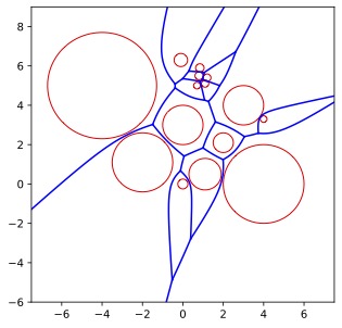
Figure 2. The Apollonius diagram.

Corollary 4.4.

Let $\mathcal{T}_{0}=\{S_{1},S_{2},\ldots,S_{n}\}$ be a set of spheres in $\mathbb{R}^{d}.$ The Voronoi diagram $\operatorname{Vor}(\mathcal{T}_{0})$ is described by Theorem 2.2 using the data sets $(\mathcal{P}^{-},\mathcal{P}^{+},\mathcal{H},\mathcal{S},\mathcal{T})$, with $\mathcal{T}=\mathcal{T}_{0}$, and with the remaining data sets empty. The corresponding system of inequalities is

$$\langle\sigma_{i},\sigma\rangle\leq 0\text{ for $i=1,\ldots,n$}.$$

Proof.

Let $\mathbf{x}$ be in the domain $\operatorname{Dom}(\mathcal{T})$. For any $i,$ let $f_{i}(\mathbf{x})==\operatorname{dist}(\mathbf{x},S_{i}(\mathbf{q}_{i},r_{i}))$. Fix $j\in[n].$ The function $f_{j}$ is minimized by $\mathbf{x}$ if and only if among all the spheres $S(\mathbf{x},r)\subseteq\operatorname{Dom}(\mathcal{T})$ , there is a sphere centered at $x$ externally tangent to $S(\mathbf{q}_{j},r_{j})$. This is equivalent to Condition (5) holding for all $i$ and holding extremally for the index $j$; or, in Lie sphere coordinates,

$$\langle\sigma_{i},\sigma\rangle\leq 0\text{ for $i=1,\ldots,n$},$$

with equality for the equation indexed by $j.$ ∎

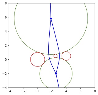
Figure 3. The Voronoi diagram for three small circles (in red). Here the minimization region for the index set $\{1,2,3\}$ is the disjoint union of two points, reflecting the fact that the intersection of the corresponding subspace in $\mathbb{R}^{5}$ intersects the Lie quadric in two distinct points.

When sites are spheres, there may be multiple edges between two vertices of the generalized Voronoi diagram. Note $\operatorname{Cell}({1,2,3})$ has is a set of cardinality two in Figure 3.

Corollary 4.5 ([Aur87]).

Let $\mathcal{S}_{0}=\{S(\mathbf{q}_{i},r_{i})\}$ be a set of $n$ spheres in $\mathbb{R}^{d}$ whose interiors are mutually disjoint. The power diagram for $\mathcal{S}_{0}$ is described by Theorem 2.2 using the data set $(\mathcal{P}^{-},\mathcal{P}^{+},\mathcal{H},\mathcal{S},\mathcal{T})$, where $\mathcal{S}=\mathcal{S}_{0}$ and the remaining sets $\mathcal{P}^{-},\mathcal{P}^{+},\mathcal{H}$ and $\mathcal{T}$ are empty. The corresponding system of inequalities is

$$\langle\sigma_{\mathbf{q}_{i},r_{i}}^{\prime},\sigma\rangle\leq 0\text{ for $i=1,\ldots,n$},$$

where $\sigma_{\mathbf{q}_{i},r_{i}}$ is the Lie sphere coordinates for the sphere $S_{i}$, in standard form.

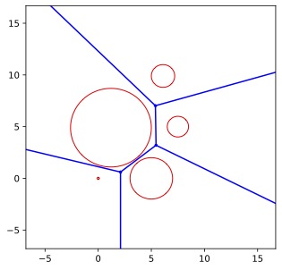
Figure 4. Power diagram

We will view the power diagram in terms of centers of maximally mostly hollow spheres, where the sphere $S(\mathbf{p},r)$ is considered mostly hollow relative to $S(\mathbf{q},t)$ if $\|\mathbf{p}-\mathbf{q}\|^{2}-r^{2}-t^{2}\geq 0,$ or equivalently, $(\sigma_{\mathbf{p},r},\sigma_{\mathbf{q},t})\leq 0.$ This occurs if and only if

$$\langle\sigma_{\mathbf{p},r}^{\prime},\sigma_{\mathbf{q},t}\rangle=(\sigma_{\mathbf{p},r},\sigma_{\mathbf{q},t})=-\textstyle{\frac{1}{2}}(\operatorname{pow}(\mathbf{p},S(\mathbf{q},t))-r^{2})\leq 0$$

Thus, the sphere $S(p,r)$ is mostly hollow relative to $S(\mathbf{p}_{1},r_{1})$ if and only if $\operatorname{pow}(\mathbf{p},S(\mathbf{p}_{1},r_{1}))\geq r^{2}$.

Proof.

Let $\mathcal{S}_{0}=\{S(\mathbf{q}_{i},r_{i})\}$ be a set of spheres as in the statement of the theorem. Let $\mathbf{p}$ be a point so that

$$R_{\mathbf{p}}:=\operatorname{pow}(\mathbf{p},S(\mathbf{p}_{j},r_{j}))=\min_{i}\operatorname{pow}(\mathbf{p},S(\mathbf{p}_{i},r_{i})).$$

Because $\mathbf{p}\not\in\cup_{i}\operatorname{int}S(\mathbf{p}_{i},r_{i})$, we know that $R_{\mathbf{p}}\geq 0.$ Then $S(\mathbf{p},R_{\mathbf{p}})$ is a maximally hollow sphere about $\mathbf{p}$ and$\langle\sigma_{\mathbf{p}_{j},r_{j}}^{\prime},\sigma_{\mathbf{p},r_{\mathbf{p}}}\rangle\leq 0.$ ∎

Next we apply Theorem 2.2 to the medial axis of a convex polygon.

Corollary 4.6.

Let $T=\cup H_{\mathbf{n}_{i},h_{i}}^{+}$ be a polyhedron defined as the intersection of half-spaces $H_{\mathbf{n}_{i},h_{i}}^{+},$ for $i\in[n]$. Let $\pi_{\mathbf{n}_{i},h_{i}}$ be the standard Lie coordinates for the half-space $H_{\mathbf{n}_{i},h_{i}}^{+}.$ The medial axis for $T$ is defined by Theorem 2.2 using the data set $(\mathcal{P}^{-},\mathcal{P}^{+},\mathcal{H},\mathcal{S},\mathcal{T})$, where $\mathcal{P}^{-},\mathcal{P}^{+},\mathcal{S}$ and $\mathcal{T}$ are empty and $\mathcal{H}=\{\pi_{\mathbf{n},h}\}$ The corresponding system of inequalities is inequalities is

$$\langle\xi_{i},\pi_{\mathbf{n},h}\rangle\leq 0\text{ for $i=1,\ldots,n$}.$$

See Figure 5.

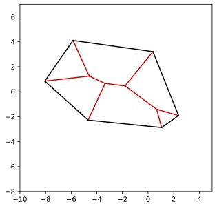
Figure 5. The medial axis of a convex polygon

Proof.

A point $\mathbf{x}$ in $\mathbb{R}^{d}$ is in the medial axis for $T$ if and only if there is a hypersphere (outwardly oriented) centered at $\mathbf{x}$ which is tangent to two or more of the oriented hyperplanes $H_{\mathbf{n}_{i},h_{i}}$. ∎

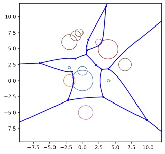
Figure 6. Mixed sites, as described in Example 4.7.

Example 4.7.

In Figure 6 we show an example where the sites in $\mathcal{D}$ are of mixed type. In fact, we have allowed some sites to be unions of objects, and removed edges accordingly to obtain the minimization diagram. Objects of the same color are considered to be part of the same generalized site.

5. Minimization diagrams from restrictions of affine functions

5.1. Observations about minimization diagrams for compositions of affine functions and embeddings.

Before we state the next theorem we make some simple observations about minimization diagrams involving embeddings and intersections.

Suppose that $\{L_{i}\}$ is a family of affine functions from $\mathbb{R}^{n}$ to $\mathbb{R}.$ The minimization diagram for the functions in $\mathcal{L}=\{L_{i}\}$ is straightforward to compute as the functions are affine; each cell is the intersection of half-spaces. Suppose that $N$ is a closed subset of $\mathbb{R}^{n}.$ For each affine function $L_{i},$ let $L_{i}|_{N}:N\to\mathbb{R}$ denote its restriction to $N$, and let $\mathcal{L}^{N}=\{L_{i}|_{N}\}$. Each minimization region for the minimization diagram $\operatorname{MD}(\mathcal{L}^{N})$ is the intersection of $N$ with the corresponding minimization region for $\operatorname{MD}(\mathcal{L})$: The minimization region $\operatorname{MR^{N}}(I)$ in $\operatorname{MD}(\mathcal{L}^{N})$ for an index set $I$ as defined in Equation (3.2) is equal to the intersection of $N$ with the corresponding polyhedral cell in $\operatorname{MD}(\mathcal{L})$. To be precise,

(5.1) $$\operatorname{MD}(\mathcal{L}^{N})=\{\overline{\operatorname{MR^{N}}(I)}\}=\{N\cap\overline{\operatorname{MR(I)}}\,:\overline{\operatorname{MR(I)}}\in\operatorname{MD}(\mathcal{L})\},$$

where $I$ varies over all possible sets of indices. Thus, the minimization diagram $\operatorname{MD}(\mathcal{L}^{N})$ for the family of functions $\mathcal{L}^{N}=\{L_{i}|_{N}\}$ may be obtained intersecting the polyhedra in $\operatorname{MD}(\mathcal{L})$ with $N.$

Figure 7. Functions $f_{i}$ factor through affine maps $L_{i}$

Next, suppose that there is an embedding $\phi:\mathbb{R}^{d}\to\mathbb{R}^{n}$, where $n>d$, and suppose that the image $N=\phi(\mathbb{R}^{d})$ is closed. Let $\mathcal{F}=\{f_{i}\}$ be a set of real-valued functions with common domain $\mathbb{R}^{d}$ such that each one is the composition $f_{i}=L_{i}\circ\phi$, where $L_{i}:\mathbb{R}^{n}\to\mathbb{R}$ is an affine function. See Figure 7. In this situation, for all $\mathbf{x}$ in $\mathbb{R}^{d},$

$$\min_{i}\{f_{i}(\mathbf{x})\}=\min_{i}\{(L_{i}\circ\phi)(\mathbf{x})\}=\min_{i}\{L_{i}(\mathbf{y})\},$$

where $\mathbf{y}=\phi(\mathbf{x})$. As a consequence, the sets of minimizing indices coincide; in the notation as in Equation (3.1), the set $I(\mathbf{x})$ for $\mathcal{F}$ equals the set $I(\phi(\mathbf{x}))$ for $\mathcal{L}=\{L_{i}\}$. Hence, $\mathbf{x}$ is in the minimization region $\operatorname{MR^{\mathcal{F}}}(I)$ for $\{f_{i}\}$ if and only if $\phi(\mathbf{x})$ is in the minimization region $\operatorname{MR^{N}}(I)$ for $\{L_{i}|_{N}\}.$ It follows that for any index set $I$, the minimization region $\operatorname{MR^{\mathcal{F}}}(I)$ is equal to the preimage $\phi^{-1}({\operatorname{MR^{N}}}(I))$ of the corresponding minimization region in $N$. We rewrite using Equation (5.1) to obtain

$$\operatorname{MR^{\mathcal{F}}}(I)=\phi^{-1}(\operatorname{MR^{N}}(I))=\phi^{-1}(N\cap\overline{MR(I)}).$$

Note that $\overline{\operatorname{MR^{\mathcal{F}}}(I)}=\overline{\phi^{-1}(\operatorname{MR^{N}}(I))}=\phi^{-1}(\overline{\operatorname{MR^{N}}(I)})$ as $\phi$ was assumed to be an embedding. We conclude that the miniization diagram for $\mathcal{F}$ is

$$\operatorname{MD}(\mathcal{F})=\{\overline{\phi^{-1}(\operatorname{MR^{N}}(I))}\}=\{\phi^{-1}(N\cap\overline{\operatorname{MR(I)}})\,:\overline{\operatorname{MR(I)}}\in\operatorname{MD}(\mathcal{L})\},$$

where $I$ varies over all possible sets of indices. The upshot of this discussion is that the minimization diagram for $\mathcal{F}$ may be computed by first finding the polyhedral minimization regions for $\operatorname{MD}(\mathcal{L})$, and then for each of these regions, intersecting with $N$ and taking the pre-image under $\phi.$ The following proposition states this precisely.

Proposition 5.1.

Let $\phi:\mathbb{R}^{d}\to\mathbb{R}^{n}$ be an embedding of $\mathbb{R}^{d}$ into $\mathbb{R}^{n}$ with closed image $N$. Let $\mathcal{F}=\{f_{i}\}_{i=1}^{n}$ be a family of real-valued functions with domain $\mathbb{R}^{N}$. Suppose that for each $i$ there is an affine function $L_{i}:\mathbb{R}^{n}\to\mathbb{R}$ so that $f_{i}=L_{i}\circ\phi.$ The minimimization diagram for $\mathcal{F}$ is the set of minimization regions

$$\operatorname{MD}(\mathcal{F})=\{\overline{\phi^{-1}(\operatorname{MR^{N}}(I))}\}=\{\phi^{-1}(N\cap\overline{\operatorname{MR(I)}})\,:\overline{\operatorname{MR(I)}}\in\operatorname{MD}(\mathcal{L})\}.$$

Now we are set to prove Theorem 2.4.

Proof of Theorem 2.4.

Let $\mathcal{F}=\{f_{i}\}_{i=1}^{n}$ and $\mathcal{L}=\{L_{i}\}_{i=1}^{n}$ be as in the statement of the theorem. Let $N=Q^{d}.$ ∎

Next we prove Proposition 2.5.

Proof of Proposition 2.5.

Let $f:\mathbb{R}^{d}\to\mathbb{R}$ be a function of form

$$f(\mathbf{x})=a\|\mathbf{x}-\mathbf{q}\|^{2}+\mathbf{b}\cdot\mathbf{x}+c,\quad\text{for $\mathbf{x}\in\mathbb{R}^{d}$},$$

where $a,c\in\mathbb{R}$ and $\mathbf{b}\in\mathbb{R}^{d}$. We rewrite $f(\mathbf{x})$ as

(5.2) $$f(\mathbf{x}) =a\|\mathbf{x}\|^{2}-2a\,\mathbf{q}\cdot\mathbf{x}+a\|\mathbf{q}\|^{2}+\mathbf{b}\cdot\mathbf{x}+c$$

$$=a\|\mathbf{x}\|^{2}+(\mathbf{b}-2a\mathbf{q})\cdot\mathbf{x}+a\|\mathbf{q}\|^{2}+c.$$

We make a linear change of variables from parameters $(a,\mathbf{b},c)$ to $\mathbf{a}=(a_{i})$ in $\mathbb{R}^{d+3}$ by letting

(5.3) $$\begin{split}\begin{bmatrix}a_{1}\\ a_{2}\end{bmatrix}&=\begin{bmatrix}-1&-1\\ -1&1\end{bmatrix}\begin{bmatrix}a\\ a\|\mathbf{q}\|^{2}+c\end{bmatrix},\\ (a_{3},\ldots,a_{d+2})&=\mathbf{b}-2a\mathbf{q},\enskip\text{and}\\ a_{d+3}&=0.\end{split}$$

This allows us to rewrite $f$ as

(5.4) $$f(\mathbf{x})=\textstyle{\frac{1}{2}}(a_{2}-a_{1})-\textstyle{\frac{1}{2}}(a_{2}+a_{1})\|\mathbf{x}\|^{2}+(a_{3},\ldots,a_{d+2})\cdot\mathbf{x}.$$

Recall that the image of a point $\mathbf{x}$ in $\mathcal{R}$ under $\phi$ is

$$\phi(\mathbf{x})=\left(\frac{1+\mathbf{x}\cdot\mathbf{x}}{2},\frac{1-\mathbf{x}\cdot\mathbf{x}}{2},\mathbf{x},0\right).$$

A short computation shows that $f(\mathbf{x})=\langle\phi(\mathbf{x}),\mathbf{a}\rangle$ where $\langle\cdot,\cdot\rangle$ is the Lie inner product. Hence

$$f(\mathbf{x})=\langle\phi(\mathbf{x}),\mathbf{a}\rangle=L_{\mathbf{a}}(\phi(\mathbf{x}))=(L_{\mathbf{a}}\circ\phi)(\mathbf{x})$$

where $L_{\mathbf{a}}$ is the linear function from $\mathbb{R}^{d+3}$ to $\mathbb{R}$ with $L_{\mathbf{a}}(\mathbf{y})=\langle\mathbf{y},\mathbf{a}\rangle$. This we have shown $f=L_{\mathbf{a}}\circ\phi.$

Conversely, given a linear function $L_{\mathbf{a}}:\mathbb{R}^{d+3}\to\mathbb{R}$ with $L_{\mathbf{a}}(\mathbf{y})=\langle\mathbf{y},\mathbf{a}\rangle$, we may partially invert Equation (5.3), ignoring the $a_{d+3}$ term, to associate to $\mathbf{a}$ the function $f(\mathbf{x})$ as in Equation (5.4) which has the property $f=L_{\mathbf{a}}\circ\phi.$ ∎

5.2. Well-known diagrams obtained from Theorem 2.4

Many kinds of diagrams meet the hypotheses of Theorem 2.4, including some familiar ones.

Proposition 5.2.

The following kinds of diagrams can be obtained as minimization diagrams as described in Theorem 2.4:

1. The classical Voronoi diagram for point sites in $\mathbb{R}^{d}$;

2. Farthest point Voronoi diagrams for point sites in $\mathbb{R}^{d}$;

3. Power diagrams defined by a set of spheres in $\mathbb{R}^{d}$;

4. Multiplicatively weighted Voronoi diagrams for point sites in $\mathbb{R}^{d}$; and

5. The medial axis of a convex polygon.

Proof.

Let $\mathcal{P}=\{\mathbf{p}_{1},\mathbf{p}_{2},\ldots,\mathbf{p}_{m}\}$ be a set of points in $\mathbb{R}^{d}.$ For each $i,$ let the function $f_{i}(\mathbf{x})=\|\mathbf{x}-\mathbf{p}_{i}\|^{2}$ be the squared distance to the point $\mathbf{p}_{i}$.

The classical Voronoi diagram with sites in $\mathcal{P}$ is the minimization diagram for the family $\mathcal{F}=\{f_{i}\}$ of squared distance functions. By Proposition 2.5, these functions meet the hypotheses of Theorem 2.4.

The farthest point Voronoi diagram with sites in $\mathcal{P}$ is the minimization diagram for $-\mathcal{F}=\{-f_{i}\,:\,f_{i}\in\mathcal{F}\}$, the family of the negatives of the squared distance functions.

The power diagram for a set of spheres $\{S_{i}\}$ in $\mathbb{R}^{d}$, by definition, is the minimization diagram for the power functions as defined in Equation (3.3). The form of the power function $\operatorname{pow}(\mathbf{x},S)=\|\mathbf{x}-\mathbf{q}\|^{2}-r^{2}$ for a sphere $S=S(\mathbf{q},r)$ meets the hypotheses of Theorem 2.4.

The multiplicatively weighted Voronoi diagram for the points $\mathcal{P}$ with positive weights $w_{1},\ldots,w_{m}$ is the minimization diagram for the nonnegative functions $\frac{1}{w_{i}}\|\mathbf{x}-\mathbf{p}_{i}\|$. (See [Aur87], Section 6.3). Equivalently, it is the minimization diagram for the functions $\frac{1}{w_{i}^{2}}\|\mathbf{x}-\mathbf{p}_{i}\|^{2}$. The squared functions meet the hypotheses of Theorem 2.4.

Let $P$ be a convex polygon defined by inequalities $\mathbf{x}\cdot\mathbf{a}_{i}\geq h$ for $i=1,\ldots,m$. The medial axis is the minimization diagram for the functions $\mathbf{x}\cdot\frac{1}{\|\mathbf{a}_{i}\|}\mathbf{a}_{i}-\frac{1}{\|\mathbf{a}_{i}\|}h$. These are of the form in the hypotheses of Theorem 2.4. ∎

5.3. Order $k$ minimization diagrams.

In this subsection we will show that Theorem 2.4 applies to order $k$ minimization diagrams. Before we prove Proposition 2.6, we make some definitions and observations involving order $k$ minimization diagrams. Let $\mathcal{F}=\{f_{1},f_{2},\ldots,f_{m}\}$ be a set of continuous functions mapping $\mathbb{R}^{d}$ to $\mathbb{R}$. Let $k\in[m]$. For any subset $\{i_{1},i_{2},\ldots,i_{k}\}$ of $[m]$ of cardinality $k$, define the function $f_{i_{1},i_{2},\ldots,i_{k}}:\mathbb{R}^{d}\to\mathbb{R}$ by

(5.5) $$f_{i_{1},i_{2},\ldots,i_{k}}(\mathbf{x})=f_{i_{1}}(\mathbf{x})+f_{i_{2}}(\mathbf{x})+\cdots+f_{i_{k}}(\mathbf{x}).$$

Let $\mathcal{F}^{k}$ be the collection of the $(\begin{smallmatrix}m\\ k\end{smallmatrix})$ functions $f_{i_{1},i_{2},\ldots,i_{k}}$:

$$\mathcal{F}^{k}=\{f_{i_{1},i_{2},\ldots,i_{k}}\,:\,1\leq i_{1}<i_{2}<\cdots i_{k}\leq m\}.$$

The next proposition states that the cells of the order $k$ Voronoi diagram $\operatorname{Vor}^{k}(\mathcal{F})$ for $\mathcal{F}$ are the same as the cells in the standard minimization diagram $\operatorname{MD}(\mathcal{F}^{k})$ for $\mathcal{F}^{k}$.

Proposition 5.3.

Let $\mathcal{F}=\{f_{1},f_{2},\ldots,f_{m}\}$ be a set of continuous functions mapping $\mathbb{R}^{d}$ to $\mathbb{R}$, let $k\in[m]$, and let $\mathcal{F}^{k}$ be as defined above. There is a one-to-one correspondence between the cells in the order $k$ minimization diagram $\operatorname{Vor}^{k}(\mathcal{F})$ for $\mathcal{F}$ and the cells in the minimization diagram $\operatorname{MD}(\mathcal{F}^{k})$ for $\mathcal{F}^{k}$. The cell for the $k$ functions $f_{i_{1}},f_{i_{2}},\cdots,f_{i_{k}}$ in the order $k$ minimization diagram for $\mathcal{F}$ is equal to the minimization region for the single function $f_{i_{1},i_{2},\ldots,i_{k}}$ in $\operatorname{MD}(\mathcal{F}^{k}).$

Proof.

Fix $\mathbf{x}\in\mathbb{R}^{d}$ and $k\in[m]$. Suppose that $\mathbf{x}$ is in the order $k$ Voronoi cell for $f_{j_{1}},\ldots,f_{j_{k}}$ in the order $k$ minimization diagram for $\mathcal{F},$ where $f_{j_{1}}(\mathbf{x})\leq f_{j_{2}}(\mathbf{x})\leq\cdots\leq f_{j_{k}}(\mathbf{x}).$ Extend this ordering to include all the values $f_{1}(\mathbf{x}),\ldots,f_{m}(\mathbf{x})$:

$$f_{j_{1}}(\mathbf{x})\leq f_{j_{2}}(\mathbf{x})\leq\cdots\leq f_{j_{m}}(\mathbf{x}),$$

where $(j_{1},j_{2},\ldots,j_{m})$ is a permutation of the set $[m].$ It follows directly from this that $f_{j_{1},j_{2},\ldots,j_{k}}(\mathbf{x})\leq f_{i_{1},i_{2},\ldots,i_{k}}(\mathbf{x})$ for all subsets $\{i_{1},i_{2},\ldots,i_{k}\}$ of $[m]$. Hence $\mathbf{x}$ is in the minimization region for $f_{j_{1},j_{2},\ldots,j_{k}}(\mathbf{x})$.

For the converse, suppose that $\mathbf{x}$ minimizes for the function $f_{j_{1},j_{2},\ldots,j_{k}}$. Then

(5.6) $$f_{j_{1},j_{2},\ldots,j_{k}}(\mathbf{x})\leq f_{i_{1},i_{2},\ldots,i_{k}}(\mathbf{x})$$

for all subsets $\{i_{1},i_{2},\ldots,i_{k}\}$ of cardinality $k$. We want to show that $f_{j_{1}}(\mathbf{x}),f_{j_{2}}(\mathbf{x}),\ldots,f_{j_{k}}(\mathbf{x})$ are the $k$ smallest values of $f_{i}(\mathbf{x}),$ for $i\in[m].$ Were this not true, then there would be some $r\not\in\{j_{1},\ldots,j_{k}\}$ so that $f_{r}(\mathbf{x})<f_{j_{i}}(\mathbf{x})$ for some $i\in\{1,2,\ldots,k\}.$ Without loss of generality, suppose that $f_{r}(\mathbf{x})<f_{j_{1}}(\mathbf{x})$. But then $f_{r,j_{2},\ldots,j_{k}}(\mathbf{x})<f_{j_{1},j_{2},\ldots,j_{k}}(\mathbf{x})$, a contradiction to (5.6). ∎

Proposition 2.6 is an immediate consequence of Proposition 5.3.

Proof of Proposition 2.6..

Let $\mathcal{F}=\{f_{i}\}$ be a family of continuous real-valued functions of form $a\|\mathbf{x}-\mathbf{q}\|^{2}+\mathbf{b}\cdot\mathbf{x}+c$ as in the statement of the proposition. Let $\mathcal{F}^{k}=\{f_{{i_{1},i_{2},\ldots,i_{k}}}\}$ be the family of functions defined by $\mathcal{F}$ as in Equation (5.5). A function of form $a\|\mathbf{x}-\mathbf{q}\|^{2}+\mathbf{b}\cdot\mathbf{x}+c$ is a multinomial of degree two or less whose order two terms are $ax_{1}^{2},\ldots,ax_{d}^{2}$ for some real number $a$. The sum of functions of this form are still of the same form. Hence the functions $f_{{i_{1},i_{2},\ldots,i_{k}}}$ are of that form, and Theorem 2.4 applies to the minimization diagram $MD(\mathcal{F}^{k})$ for $\mathcal{F}^{k}.$ By Proposition 5.3, the cells of the order $k$ Voronoi diagram for $\mathcal{F}$ are the cells of $MD(\mathcal{F}^{k}).$ ∎

6. Algorithm

The algorithm is for computing the minimization diagram for a set $S$ of functions given by linear conditions in Lie sphere coordinates for Lie spheres in $\mathbb{R}^{d}.$ Following is the algorithm to compute the generalized Voronoi diagram.

Data: Sites $S$

Result: Voronoi vertices and connectivity

1 Map $S$ to canonical Lie sphere coordinates;

2 Do change of variables on $S$;

3 Compute and map bounding box;

4 Compute and map feasible point using bounding box;

5 Compute convex hull of Lie sphere coordinates by intersecting half-spaces in $\mathbb{R}^{d+2}$;

6 Get 1-dimensional faces $f$ between convex hull vertices;

7 Filter out edges with two bounding box equations;

8 Solve linear inequalities to find the voronoi edges;

9 Intersect edges with Lie quadric to find voronoi vertices (not medial axis);

Let $n$ be $|S|$. Lines 1 and 2 of the algorithm are $O(nd)$. Lines 3 and 4 are $O(d)$. The Lie sphere coordinates are in $\mathbb{R}^{d+2}$. Line 5, the intersection of half-spaces, uses the incremental convex hull algorithm, which is $\mathcal{O}(n\log{n}+n^{\lfloor\frac{d+3}{2}\rfloor})$ ([BCY18, p. 59]). For Line 6, assume the sites are in general position. Each vertex $p$ is “included in exactly $d+2$ of the bounding hyperplanes” ([BCY18, p. 54]). Then the number of 1-dimensional faces incident to each vertex $p$ is $d+2$. If there are $n$ hyperplanes, then there are $n(d+2)/2=\mathcal{O}(nd)$ 1-dimensional faces. Line 7 is $O(nd)$. In Line 8, to find the Voronoi edges, we solve a system of $d+1$ linear inequalities of half-spaces for each 1-dimensional face which is $O(nd^{2})$. Line 9 is $O(nd)$. The algorithm is dominated by lines 5 and 8, yielding $\mathcal{O}(n\log{n}+n^{\lfloor\frac{d+3}{2}\rfloor}+nd^{2})$.

References

- [ADK06] Franz Aurenhammer, Robert L Scot Drysdale, and Hannes Krasser, Farthest line segment Voronoi diagrams, Information Processing Letters 100 (2006), no. 6, 220–225.
- [AE84] F. Aurenhammer and H. Edelsbrunner, An optimal algorithm for constructing the weighted Voronoi diagram in the plane, Pattern Recognition 17 (1984), no. 2, 251–257. MR 765066
- [AKL13] Franz Aurenhammer, Rolf Klein, and Der-Tsai Lee, Voronoi diagrams and Delaunay triangulations, 2013.
- [Aur87] Franz Aurenhammer, Power diagrams: properties, algorithms and applications, SIAM Journal on Computing 16 (1987), no. 1, 78–96.
- [Aur91] by same author, Voronoi diagrams—a survey of a fundamental geometric data structure, ACM Computing Surveys (CSUR) 23 (1991), no. 3, 345–405.
- [BCY18] Jean-Daniel Boissonnat, Frédéric Chazal, and Mariette Yvinec, Geometric and topological inference, vol. 57, Cambridge University Press, 2018.
- [Bro79] Kevin Q Brown, Voronoi diagrams from convex hulls, Information processing letters 9 (1979), no. 5, 223–228.
- [Cec] Thomas E. Cecil, Lie sphere geometry, second ed., Universitext.
- [D+34] Boris Delaunay et al., Sur la sphere vide, Izv. Akad. Nauk SSSR, Otdelenie Matematicheskii i Estestvennyka Nauk 7 (1934), no. 793-800, 1–2.
- [dBvKOS97] Mark de Berg, Marc van Kreveld, Mark Overmars, and Otfried Schwarzkopf, Computational geometry, pp. 147–148, 254, 1997.
- [DMT92] Olivier Devillers, Stefan Meiser, and Monique Teillaud, The space of spheres, a geometric tool to unify duality results on Voronoi diagrams, Ph.D. thesis, INRIA, 1992.
- [DO11] Satyan L Devadoss and Joseph O’Rourke, Discrete and computational geometry, Princeton University Press, 2011.
- [ES86] Herbert Edelsbrunner and Raimund Seidel, Voronoi diagrams and arrangements, Discrete & Computational Geometry 1 (1986), no. 1, 25–44.
- [Ros91] Harald Rosenberger, Order-k Voronoi diagrams of sites with additive weights in the plane, Algorithmica 6 (1991), no. 1, 490–521.