Counterfactual and Synthetic Control Method: Causal Inference with Instrumented Principal Component Analysis

The fundamental problem of causal inference lies in the absence of counterfactuals. Traditional methodologies impute the missing counterfactuals implicitly or explicitly based on untestable or overly stringent assumptions. Synthetic control method (SCM) utilizes a weighted average of control units to impute the missing counterfactual for the treated unit. Although SCM relaxes some strict assumptions, it still requires the treated unit to be inside the convex hull formed by the controls, avoiding extrapolation. In recent advances, researchers have modeled the entire data generating process (DGP) to explicitly impute the missing counterfactual. This paper expands the interactive fixed effect (IFE) model by instrumenting covariates into factor loadings, adding additional robustness. This methodology offers multiple benefits: firstly, it incorporates the strengths of previous SCM approaches, such as the relaxation of the untestable parallel trends assumption (PTA). Secondly, it does not require the targeted outcomes to be inside the convex hull formed by the controls. Thirdly, it eliminates the need for correct model specification required by the IFE model. Finally, it inherits the ability of principal component analysis (PCA) to effectively handle high-dimensional data and enhances the value extracted from numerous covariates.

Keywords: Synthetic Control, Principal Component Analysis, Causal Inference

JEL Codes: G11, G12, G30

1 Introduction

In this paper, we introduce a novel counterfactual imputation method called the Counterfactual and Synthetic Control method with Instrumented Principal Component Analysis (CSC-IPCA). This method combines the dimension reduction capabilities of PCA (Jollife and Cadima (2016)) to handle high-dimensional datasets with the versatility of the factor model (Bai and Perron (2003); Bai (2009)) which accommodates a wide range of data generating processes. Our approach aligns with the previously proposed Counterfactual and Synthetic Control method with Interactive Fixed Effects (CSC-IFE) by Xu (2017). The CSC-IPCA method models the entire DGP, overcoming constraints imposed by untestable and stringent assumptions such as unconfoundedness and common support for matching (Rosenbaum and Rubin (1983); Rubin (1997)), and the parallel trend assumption for difference-in-differences (DID) (Card and Krueger (1993)). Additionally, it addresses limitations found in the original SCM (Abadie et al. (2010)) and its variants (Ben-Michael et al. (2021), Arkhangelsky et al. (2021)), which require the outcomes of treated units to lie inside or not far from the convex hull formed by the controls.

Causal inference in economics and other social sciences is frequently complicated by the absence of counterfactuals, which are essential for evaluating the impact of a treatment or policy intervention. Imbens and Rubin (2015) state that, at some level, all methods for causal inference can be viewed as missing data imputation methods, although some are more explicit than others. For instance, under certain assumptions, the matching method (Abadie and Imbens (2006, 2011)) explicitly imputes the missing counterfactual for treated units with meticulously selected controls. The DID method (Card and Krueger (1993); Ashenfelter (1978)), on the other hand, implicitly imputes the missing counterfactual by differencing the control units before and after treatment. Meanwhile, the SCM method explicitly imputes the missing counterfactual with a weighted average of control units. Our method aligns with the recent trend in the causal inference literature, aiming to explicitly impute the missing counterfactual by modeling the entire DGP, a strategy highlighted by Athey et al. (2021) with their matrix completion (MC) method, and Xu (2017) with their CSC-IFE method.

Factor models have long been explored in the econometrics literature related to modeling panel data, with significant contributions by Bai and Perron (2003), Pesaran (2006), Stock and Watson (2002), Eberhardt and Bond (2009), among others. However, within the context of causal inference, Hsiao et al. (2012) stands out as the first work proposing the use of these methods specifically for predicting missing counterfactuals in synthetic control settings, followed by Gobillon and Magnac (2016), Xu (2017), Chan et al. (2016), and Li (2018). The CSC-IPCA estimator builds upon the instrumented principal component analysis first introduced by Kelly et al. (2020) and Kelly et al. (2019) in the context of predicting stock returns. It belongs to the factor model family; through the instrumented factor loadings, we can estimate the latent factors more accurately, and the instrumented factor loadings will inherit time-varying properties, offering better economic interpretation. Firstly, it assumes a simple factor model, as in Bai and Perron (2003), with only the structural component between factor loadings $\Lambda_{i}$ and factors $F_{t}$:

$$Y_{it}=\Lambda_{i}F^{\prime}_{t}+\mu_{it}$$ (1)

Secondly, it instruments the factor loadings $\Lambda_{i}$ with covariates $X_{it}$, which allows us to capture the time-varying properties of the factor loadings:

$$\Lambda_{it}=X_{it}\Gamma+H_{it}$$ (2)

The static factor loadings $\Lambda_{i}$ in Equation 1 are assumed to be time-invariant by most studies in the related literature. However, in many economic and social science contexts, the factor loadings are not constant but fluctuate over time in response to relevant covariates. This adaptation is particularly realistic in many economic and social science contexts. By instrumenting the factor loadings $\Lambda_{i}$ with covariates $X_{it}$ through Equation 2, we can capture the time-varying properties of the factor loadings. The matrix $\Gamma$, serving as an $L\times K$ mapping function from covariates (number of $L$) to factor loadings (number of $K$), also acts as a dimension reduction operation, which aggregates all the information from the covariates into a smaller number of factors, making the model parsimonious.

The instrumented factor loadings enhance our estimation of the time-varying latent factors $F_{t}$. Unlike the prediction problem addressed in Kelly et al. (2020, 2019), here we utilize only the control units to estimate $F_{t}$ and then update $\Gamma$ with the treated units before treatment. This represents the crucial distinction between our method for causal inference and the IPCA method for prediction, where the mapping matrix $\Gamma$ is assumed to be constant for all units across all periods.

This approach offers three major advantages over the CSC-IFE model and other methods that use factor models for causal inference. First, it removes the need for correct model specification, which is a crucial requirement of the CSC-IFE method. In the CSC-IFE method, aside from the structural component $\lambda_{i}F_{t}$, it also mandates that covariates be included linearly in the functional form as regressors $X_{it}\beta$. Second, in the CSC-IPCA method, the factor loadings $\Lambda_{it}$ are instrumented by covariates, introducing time-varying characteristics to the factor loadings. This property, as we discussed, is particularly realistic in many economic and social science contexts. Third, the CSC-IPCA method includes a dimension reduction step using the matrix $\Gamma$, which is especially beneficial for high-dimensional datasets with a large number of covariates. This feature makes it particularly valuable for financial data (Feng et al. (2020)) and high-dimensional macroeconomic time series data (Brave (2009)).

This paper is structured as follows. Section 2 introduces the framework of the CSC-IPCA method, detailing the functional form and assumptions for identification. Section 3 outlines the estimation procedures, including hyperparameter tuning and inference. Section 4 presents the results of Monte Carlo simulations, comparing different estimation methods and providing finite sample properties. Section 5 demonstrates the application of the CSC-IPCA method in a real-world setting, evaluating the impact of Brexit on foreign direct investment in the U.K. Section 6 concludes the paper with a summary of the main findings and potential future research directions. More detailed proofs and derivations are provided in Appendix A.

2 Framework

Consider $Y_{it}$ as the observed outcome for a specific unit $i\ (i=1,\dots,N)$ at time $t\ (t=1,\dots,T)$. The total number of observed units in the panel is $N=N_{treat}+N_{ctrl}$, where $N_{treat}$ represents the number of units in the treatment group $\mathcal{T}$ and $N_{ctrl}$ represents the number of units in the control group $\mathcal{C}$. Each unit is observed over $T=T_{pre}+T_{post}$ periods, where $T_{pre}$ is the number of periods before treatment and $T_{post}$ is the number of periods after treatment. We observe the treatment effect at $T_{pre}+1$ right after the beginning of the treatment and continue to observe thereafter until the end of the observation periods, a scenario commonly referred to as block assignment. Following Equations 1 and 2, we assume that the outcome variable $Y_{it}$ is given by a simple factor model with factor loadings instrumented by covariates. The functional form is given by:

Assumption 1

Functional form:

$$Y_{it}=D_{it}\circ\delta_{it}+\Lambda_{it}F_{t}^{\prime}+\mu_{it},$$ (3)

$$\Lambda_{it}=X_{it}\Gamma+H_{it}$$

The primary distinction of this functional form from existing interactive fixed effects models (Gobillon and Magnac (2016); Chan et al. (2016)) is that the factor loading $\Lambda_{it}$ is instrumented by observed covariates $X_{it}$, which makes the conventionally static factor loadings exhibit time-varying features. Specifically, $F_{t}=[f_{t}^{1},\ldots,f_{t}^{K}]$ is a vector of $K$ unobserved common factors, and $\Lambda_{it}=[\lambda_{it}^{1},\ldots,\lambda_{it}^{K}]$ represents a vector of factor loadings. Meanwhile, the vector $X_{it}=[x_{it}^{1},\ldots,x_{it}^{L}]$ comprises $L$ observed covariates. The transformation matrix $\Gamma$, which is of size $L\times K$, maps the information from observed covariates $X_{it}$ to factor loadings $\Lambda_{it}$. This integration permits $\Lambda_{it}$ to exhibit variability across time and units, thereby introducing an additional layer of heterogeneity into the model. Another key difference from the CSC-IFE approach by Xu (2017) is that we retain only the interactive component $\Lambda_{it}F_{t}$ between factors and factor loadings; the linear part of covariates $X_{it}\beta$ is not included in the functional form. The logic behind this is that we believe the unit-specific factor loadings, instrumented by covariates, have included all the predictive information from these covariates. This functional form exhibits two major advantages over the CSC-IFE model. Firstly, it does not require the correct model specification, a crucial demand of the CSC-IFE method. Secondly, it incorporates a dimension reduction operation via the matrix $\Gamma$, which allows us to handle high-dimensional datasets, especially when dealing with a large number of covariates.

The remainder of the model adheres to conventional standards, where $D_{it}$ denotes a binary treatment indicator, and $\delta_{it}$ represents the treatment effect, which varies across units and over time. For computational simplicity, we assume $D_{it}=1$ for unit $i$ in the group of treated $\mathcal{T}$ and for period $t>T_{pre}$, with all other $D_{it}$ set to $0$. The model easily accommodates variations in treatment timing by removing the constraint that treatment must commence simultaneously for all treated units. The term $\mu_{it}$ signifies the idiosyncratic error associated with the outcome variable $Y_{it}$. Additionally, $H_{it}=[\eta_{it}^{1},\ldots,\eta_{it}^{K}]$ constitutes the vector of error terms linked to $K$ unobserved factor loadings.

Following Neyman (1932) potential outcome framework (also discussed by Rubin (1974, 2005)), we observe the actual outcome for the treated and untreated units:

$$\begin{cases}Y_{it}^{1}=\delta_{it}+X_{it}\Gamma F^{\prime}_{t}+\epsilon_{it}&if\ i\in\mathcal{T}\ \&\ t>T_{pre}\\ Y_{it}^{0}=X_{it}\Gamma F^{\prime}_{t}+\epsilon_{it}&otherwise.\end{cases}$$ (4)

where Equation 4 represents the actual outcome for the treated and control units combined the two parts together in Equation 3. Our goal is to impute the missing counterfactual $\hat{Y}_{it}^{0}=X_{it}\hat{\Gamma}\hat{F}_{t}$ for the treated units $i\in\mathcal{T}$ when $t>T_{pre}$, where the $\hat{\Gamma}$ and $\hat{F}_{t}$ are estimated parameters. We then calculate the treatment effect for the treated (ATT) as the difference between the actual outcome and imputed missing counterfactual, which is defined as:

$$\widehat{ATT}_{t}=\frac{1}{N_{treat}}\sum_{i\in\mathcal{T}}\left(Y_{it}^{1}-\hat{Y}_{it}^{0}\right)=\frac{1}{N_{treat}}\sum_{i\in\mathcal{T}}\hat{\delta}_{it}.$$ (5)

2.1 Assumptions for identification

To ensure the identification of the treatment effect, we introduce a series of assumptions about the DGPs, in addition to the assumption regarding the functional form. These assumptions are crucial for achieving consistent estimation of the treatment effect, yet they are easy to satisfy in practice.

Assumption 2

Assumptions for consistency:

1. Covariate orthogonality.

2. Moment condition of factors and covariates.

3. Compact parameter space for $\Gamma$.

The assumptions outlined above serve as regularity conditions necessary for ensuring the consistency of the estimator. The first condition reflects the exclusion restriction commonly associated with instrumental variable regression, indicating that the instruments (in this case, covariates) are orthogonal to the error terms. This orthogonality ensures that the covariates do not correlate with any unobserved error terms influencing the outcome. Similarly, the functional form described in Equation 3 aligns with the framework utilized in two-stage instrumental regression. The second condition imposes a limitation on the second moment of a series of random variables, ensuring that their variances remain finite and do not escalate indefinitely. The third condition mandates that the parameter space for the mapping matrix $\Gamma$ be compact, thereby circumventing issues related to rank deficiency. This compactness is vital for the estimability of $\Gamma$ and the existence of its inverse, mirroring standard factor analysis assumptions. We provide detailed explanations of each assumption’s conditions in Appendix A.2.

Assumption 3

Assumptions for asymptotic normality.

1. Panel-wise and cross-sectional central limit theorem.

2. Bounded dependence for covariates and errors.

3. Cross-sectional homoskedasticity of covariates.

To derive the asymptotic properties of the CSC-IPCA estimator, we introduce additional assumptions. Assumption 3 encompasses panel-wise and cross-sectional central limit theorems for various variables, which are fulfilled by diverse mixing processes. These conditions are pivotal for determining the asymptotic distribution of factors and mapping matrix estimations. For an in-depth discussion, we refer to Kelly et al. (2020). The requirement of bounded dependence stipulates that both time series and cross-sectional dependencies of $X_{it}\epsilon_{it}$ are bounded, a crucial step for establishing asymptotic normality. Meanwhile, the assumption of cross-sectional homoskedasticity simplifies the expressions for the asymptotic variances of the estimated mapping matrix $\Gamma$. It should be noted that relaxing this assumption would not alter the convergence rate. Detailed explanations of each assumption’s conditions are provided in Appendix Assumption A.3.

3 Estimation

The CSC-IPCA estimator of the treatment effect for a treated unit $i$ at time $t$ is defined as the difference between the observed outcome and its estimated counterfactual: $\hat{\delta}_{it}=Y_{it}^{1}-\hat{Y}_{it}^{0}$. To combine the functional form in Equation 3, we get the structural component of the potential outcome $Y_{it}=(X_{it}\Gamma)F^{\prime}_{t}$. The CSC-IPCA method is estimated by minimizing the sum of squared residuals of the following objective function:

$$\underset{\Gamma,F_{t}}{\arg\min}\sum_{i}\sum_{t}\left(Y_{it}-(X_{it}\Gamma)F^{\prime}_{t}\right)\left(Y_{it}-(X_{it}\Gamma)F^{\prime}_{t}\right)^{\prime}.$$ (6)

Unlike the IFE method (Bai (2009); Xu (2017)), our approach requires estimating only two parameters, $\Gamma$ and $F_{t}$, simplifying the process. Different from principal component analysis (Jolliffe (2002); Stock and Watson (2002)), our method involves using covariates to instrument the factor loadings. This necessitates the estimation of $\Gamma$ rather than $\Lambda_{i}$, so we can not directly use eigenvalue decomposition. While the objective function in Equation 6 formulates the problem as minimizing a quadratic function with a single unknown variable (e.g., $\Gamma$) while holding the other variable (e.g., $F_{t}$) constant. This structure enables the application of the alternating least squares (ALS) method for a numerical solution. Generally, the imputation for the missing counterfactual $Y_{it}(0)$ is executed in four steps:

Step 1: The initial step entails estimating the time-varying factors $\hat{F}_{t}$ and the mapping matrix $\hat{\Gamma}_{\text{ctrl}}$ utilizing the ALS algorithm, with the control group data exclusively for the whole period.

$$(\hat{\Gamma}_{ctrl},\hat{F_{t}})=\underset{\Gamma,F_{t}}{\arg\min}\sum_{i\in\mathcal{C}}\sum_{t\leq T}\left(Y_{it}-(X_{it}\Gamma)F^{\prime}_{t}\right)\left(Y_{it}-(X_{it}\Gamma)F^{\prime}_{t}\right)^{\prime}.$$ (7)

Step 2: The subsequent step involves estimating the mapping matrix $\hat{\Gamma}_{treat}$ for treated unit $i$ at time $t$, employing the previously estimated time-varying factors $\hat{F}_{t}$ and the observed covariates $X_{it}$, using treated group data exclusively for the pre-treatment period.

$$\hat{\Gamma}_{treat}=\underset{\Gamma}{\arg\min}\sum_{i\in\mathcal{T}}\sum_{t\leq T_{pre}}\left(Y_{it}-(X_{it}\Gamma)\hat{F}^{\prime}_{t}\right)\left(Y_{it}-(X_{it}\Gamma)\hat{F}^{\prime}_{t}\right)^{\prime}.$$ (8)

Step 3: The third step includes normalizing the estimated mapping matrix $\hat{\Gamma}_{treat}$ and factors $\hat{F_{t}}$ by a set of constraints:

$$\Gamma_{norm} =\hat{\Gamma}_{treat}R,$$ (9)

$$F_{norm} =R^{-1}\hat{F}_{t},$$

$$s.t.\Gamma_{norm}^{\prime}\Gamma_{norm} =\mathcal{I}_{K},\quad F_{norm}F_{norm}^{\prime}/T=\text{Diagonal}.$$

Similar to most factor analysis methods, the estimated $\Gamma$ and $F_{t}$ are not deterministic. There exist an infinite number of “rotated” parameters $\Gamma R$ and $R^{-1}F_{t}$ that yield the same objective function value (i.e., $X_{it}\Gamma F_{t}=X_{it}\Gamma RR^{-1}F_{t}$). To make the estimation identifiable, it is necessary to impose some constraints on the estimated $\Gamma$ and $F_{t}$. Following Connor and Korajczyk (1993); Stock and Watson (2002); Bai and Ng (2002), the aforementioned restrictions reduce the model’s complexity and make it easier to understand and interpret the relationships between the factors $F_{t}$ and factor loadings $\Lambda_{it}$. Unlike the estimation methods in Bai (2009); Xu (2017), where normalization constraints are set before the estimation, the structural component $X_{it}\Gamma F_{t}$ allows us to normalize the estimated $\Gamma$ and $F_{t}$ after the estimation. This enables us to easily find the rotation matrix $R$ that satisfies the above constraints.

Step 4: The final step involves imputing the counterfactual outcome $\hat{Y}_{it}^{0}$ for treated unit $i$ at time $t$ by substituting the estimated mapping matrix $\hat{\Gamma}_{norm}$ and the time-varying factors $\hat{F}_{norm}$ into the following equation:

$$\hat{Y}_{it}(0)=(X_{it}\hat{\Gamma}_{norm})\hat{F}^{\prime}_{norm},\quad\forall i\in\mathcal{T}\ \&\ T_{pre}<t\leq T.$$ (10)

The main difference between CSC-IPCA and the instrumented principal component analysis (IPCA) as proposed by Kelly et al. (2020) lies in the purpose of prediction. In the IPCA method, the authors predict the next period stock returns using all covariates from the preceding period, under the assumption that the mapping matrix $\Gamma$ remains constant across all observations. In contrast, CSC-IPCA introduces a pivotal distinction: it operates under the assumption that treated and control groups are characterized by unique mapping matrices, $\Gamma_{\text{treat}}$ and $\Gamma_{\text{ctrl}}$. This assumption is vital for the unbiased estimation of the ATT, setting the CSC-IPCA method apart by directly addressing heterogeneity in the treatment effect through the specification of group-specific mapping matrices. The detailed estimation procedures are presented in the Appendix A.3.

3.1 Hyper parameter tuning

Similar to CSC-IFE methods, researchers often encounter the challenge of selecting the appropriate number of latent factors, $K$, without prior knowledge of the true data generating process. To facilitate this selection, we introduce data-driven approaches for determining the hyperparameter $K$. Utilizing both control and treated units as training and validation data, respectively, offers a practical solution. To enhance the robustness of this process, we propose two validation methods for hyperparameter tuning. Algorithm 1 describes a bootstrap method to ascertain $K$. This approach involves repeatedly sampling $N_{ctrl}$ control units for training data and $N_{treat}$ treated units for validation data, both with replacement. The optimal $K$ is then determined by minimizing the average sum of squared errors across these validations. We also propose a leave-one-out cross-validation method, as detailed in Appendix A.4.

Data: $Y,X$

Result: Optimal hyperparameter $k$

1 Determine the maximum possible hyperparameter $K$ and the number of repetitions $N$;

2

3Initialize an array $MSE$ to store the average of sum squared error for each $k$;

4 for $k\leftarrow 1$ to $K$ do

5       Initialize sum of squared errors: $SSE_{k}\leftarrow 0$;

6       for $n\leftarrow 1$ to $N$ do

7             Construct a bootstrap training dataset $(Y^{b}_{ctrl},X^{b}_{ctrl})$ by sampling $N_{ctrl}$ control observations with replacement;

8            

9            Construct a bootstrap validation dataset $(Y^{b}_{treat},X^{b}_{treat})$ by sampling $N_{treat}$ treated observations with replacement;

10            

11            Estimate parameters $\Gamma$ and $F_{t}$ using the training data via the ALS method;

12            

13            Use the estimated $\hat{\Gamma}$ and $\hat{F}_{t}$ to predict $\hat{Y}^{b}_{treat}$ with the validation data;

14            

15            Compute the sum of squared error for the validation data: $SE_{n}\leftarrow\sum\left(Y^{b}_{treat}-\hat{Y}^{b}_{treat}\right)^{2}$;

16            

17            Accumulate the sum of squared errors: $SSE_{k}\leftarrow SSE_{k}+SE_{n}$;

18            

19       end for

20      Calculate the average sum squared error for $k$: $MSE[k]\leftarrow\frac{SSE_{k}}{N}$;

21      

22 end for

23Select $k$ corresponding to the minimum value in $MSE$;

Algorithm 1 Bootstrap Hyperparameter Tuning

3.2 Inference

In the context of causal inference, the pioneering application of factor models is attributed to Hsiao et al. (2012). Nonetheless, a formal framework for inference using this method was not established until the works of Chan et al. (2016) and Li (2018). These methods of inference rely on a large number of control units and pre-treatment periods to develop asymptotic properties. In recent years, conformal inference (Chernozhukov et al. (2021)) has gained popularity in the causal inference literature, as seen in Ben-Michael et al. (2021), Roth et al. (2023), and Imbens (2024). Conformal inference is a nonparametric method that provides exact and robust inference without requiring the specification of the model. Our causal inference framework, designed for predicting missing counterfactuals, allows us to construct inference procedures based on conformal prediction, as introduced by Shafer and Vovk (2008), to ensure robustness against misspecification. The causal effect is identified as the difference between the observed outcomes and these estimated counterfactuals, expressed mathematically as:

$$\theta_{it}=Y^{1}_{it}-\hat{Y}^{0}_{it},\quad\forall i\in N_{treat}\ \&\ T_{pre}+1\leq t\leq T,$$

where $\theta_{it}$ denotes the treatment effect for unit $i$ at time $t$, and $\hat{Y}_{it}$ represents the imputed counterfactual outcome.

To conduct conformal inference, we first postulate a sharp null hypothesis, $H_{0}:\theta_{it}=\theta_{it}^{0}$. Under this null hypothesis, we adjust the outcome for treated units post-treatment as $\tilde{Y}_{it}=Y_{it}-\theta_{it}$. We then replace the original dataset with this adjusted part, $\tilde{Y}_{it}$.

Secondly, we follow the estimation procedures described in Section 3 to estimate the time-varying factor $F_{t}$ using only control data, as before, and update $\Gamma$ for the newly adjusted treated units using the entire set of treated units. The concept revolves around updating $\Gamma$ using all the treated units, under the assumed null hypothesis, to minimize the occurrence of large residuals after intervention.

Thirdly, we estimate the treatment effect and compute the residuals for the treated units in the post-treatment periods. The test statistic showing how large the residual is under the null:

$$S(\hat{\mu})=\left(\frac{1}{\sqrt{T_{post}}}\sum_{t>T_{pre}}|\hat{\mu}|^{q}\right)$$ (11)

Where $\hat{\mu}$ represents the residual for the treated units in the post-treatment periods, we employ $q=1$ for the permanent intervention effect as designed in our study. A high value of the test statistic indicates a poor post-treatment fit, suggesting that the treatment effect postulated by the null is unlikely to be observed, hence leading to the null’s rejection.

Finally, we block permute the residuals and calculate the test statistic in each permutation. The P-value is defined as:

$$\hat{p}=1-\hat{F}(S(\hat{u})),\text{ where }\hat{F}(x)=\frac{1}{|\Pi|}\sum_{\pi\in\Pi}1\{S(\hat{u}_{\pi})<x\}.$$ (12)

where $\Pi$ represents the set of all block permutations, the test statistic for each permutation is denoted by $S(\hat{\mu}_{\pi})$, with $x$ being the test statistic calculated from the unpermuted residuals. By employing different sets of nulls, we can compute a confidence interval at a specified confidence level.

4 Monte Carlo Simulation

In this section, we employ Monte Carlo simulations to assess the performance of the CSC-IPCA estimator in finite sample settings. We juxtapose the CSC-IPCA estimator against the CSC-IFE and the original SCM estimators. Our comparative analysis focuses on key metrics including bias, mean squared errors, and converage properties.

In this section, we employ Monte Carlo simulations to assess the performance of the CSC-IPCA estimator in finite sample settings. We compare the CSC-IPCA estimator against the CSC-IFE and the original SCM estimators. Our comparative analysis focuses on key metrics, including bias, mean squared errors, and convergence properties.

We initiate our analysis with a data generating process that incorporates $L=10$ covariates and $K=3$ time-varying common factors, along with unit and time-fixed effects:

$$Y_{it}=D_{i}\delta^{\prime}_{t}+X_{it}\beta^{\prime}+(X_{it}\Gamma)F^{\prime}_{t}+\alpha_{i}+\xi_{t}+\epsilon_{it}.$$ (13)

where $X_{it}=[x_{it}^{1},\ldots,x_{it}^{L}]$ denotes a vector of $L\times 1$ covariates, which follows a VAR(1) process. $X_{it}=\mu_{i}+A_{i}X_{i,t-1}+\nu_{it}$, where $A_{i}$ is a $L\times L$ variance-covariance matrix, The drift term $\mu_{i}$ equals 0 for control units and 2 for treated units, and $\nu_{it}$ is a $L\times 1$ vector of i.i.d. standard normal errors. While $F_{t}=[f_{t}^{1},\ldots,f_{t}^{K}]$ denotes the vector of common factors, adhering to a similar VAR(1) process, the variable $\epsilon_{it}$ represents the idiosyncratic error term. Unit and time fixed effects, $\alpha_{i}$ and $\xi_{t}$ respectively, are uniformly drawn from the interval $(0,1)$. The coefficient vector $\beta=[\beta^{1},\ldots,\beta^{L}]$ associated with the covariates is drawn uniformly from $(0,1)$, and $\Gamma$, the $L\times K$ mapping matrix for the factor loadings, is drawn uniformly from $(-0.1,0.1)$. The treatment indicator $D_{it}$ is binary, defined as $D_{it}=1$ for treated units during post-treatment periods, and $D_{it}=0$ otherwise. The heterogeneous treatment effect is modeled as $\delta_{it}=\bar{\delta}_{it}+e_{it}$, where $e_{it}$ is i.i.d as standard normal, and $\bar{\delta_{t}}=[0,\cdots,0,1,2,\ldots,T_{post}]$ represents a time-varying treatment effect. Only the outcome $Y_{it}$, the covariates $X_{it}$, and the treatment indicator $D_{it}$ are observed, while all other variables remain unobserved.

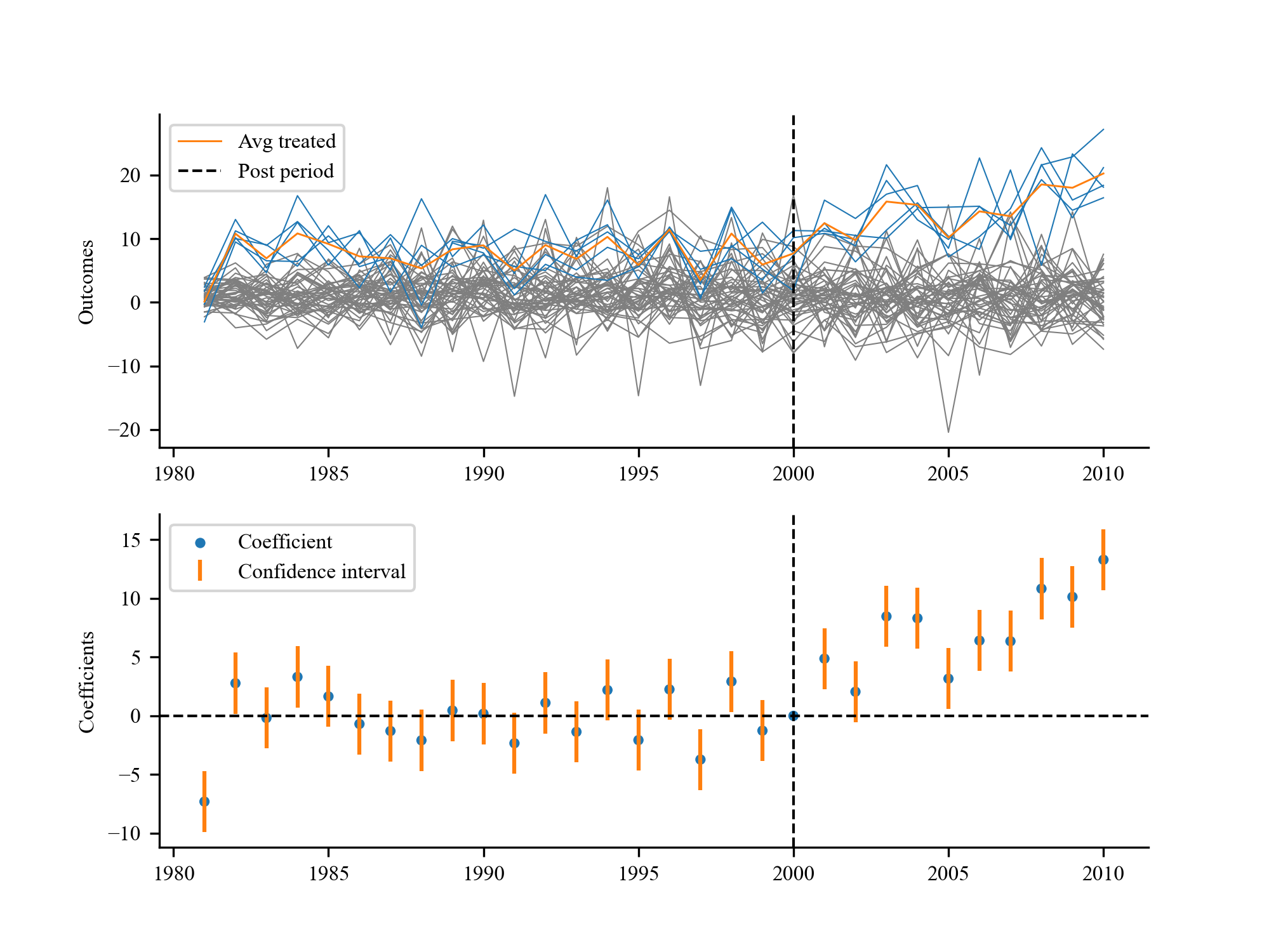
Figure 1: CSC-IPCA Data Generating Process

In this graphic, the upper panel plots simulated data following the above data generating process. The light blue lines represent treated units and the light gray lines represent controls. Key parameters are $N_{treat}=5,N_{ctrl}=45,T_{0}=20,T_{1}=10,L=10$. The lower panel plots a simple event study.

Figure 1 represents the simulated data following our data generating process. Observations from the upper panel indicate that the parallel trend assumption is not met. To verify this, we plot a simple event study, clearly revealing a failure in the parallel trend assumption. Furthermore, outcomes for treated units are marginally higher than for control units. In such cases, the synthetic control method will be biased, as it avoids extrapolation and typically fits poorly for treated units.

4.1 A simulated example

Following this data generating process, Figure 2 illustrates both the raw data and the imputed counterfactual outcomes as estimated by the CSC-IPCA method. In the upper panel, control units are represented in gray and treated units in light blue, with the average outcome for treated units highlighted in orange. The imputed synthetic average for treated outcomes is also shown, delineated by an orange dashed line. The CSC-IPCA method is capable of capturing the trajectory of the average outcome for treated units before treatment, and we observe the divergence after the treatment. The lower panel of Figure 2 shows the estimated ATT (dashed line) alongside the true ATT (solid line) and the 95% confidence interval based on conformal inference. The CSC-IPCA method is able to capture the true ATT, as evidenced by the close alignment between the dashed and solid lines. The confidence interval constructed through conformal inference is also accurate, as it encompasses the true ATT.

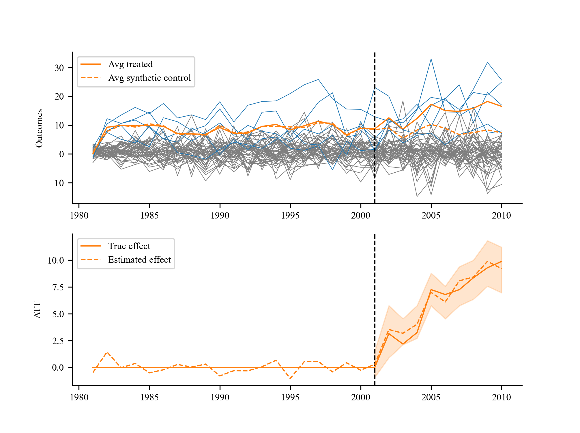
Figure 2: CSC-IPCA Estimated ATT for Simulated Sample

This graphic plots the CSC-IPCA method estimated ATT for simulated data $N_{treat}=5,N_{ctrl}=45,T_{0}=20,T_{1}=10,L=10$.

4.2 Bias comparison

Based on the same data generating process and parameters, we compare the CSC-IPCA, CSC-IFE, and SCM estimators with 1000 simulations. Figure 3 illustrates the bias among these different estimation methods. In panel 1, when all covariates are observed, both CSC-IPCA and CSC-IFE demonstrate unbiasedness and effectively estimate the true ATT. However, due to the outcomes of treated units falling outside the convex hull of control units, the SCM exhibits an upward bias, as Abadie et al. (2010) suggests that in such scenarios, SCM should be avoided. It is often the case in financial and macroeconomic studies that only a subset of covariates is observed, rather than all of them. In panels 2 and 3, we observe only 2/3 and 1/3 of the covariates, respectively. As the number of unobserved covariates increases, both CSC-IPCA and CSC-IFE lose efficiency, but the CSC-IPCA estimator remains less biased than the CSC-IFE estimator. We compare the bias of different estimators with different DGPs in Appendix C.4, and the results are consistent with the above findings.

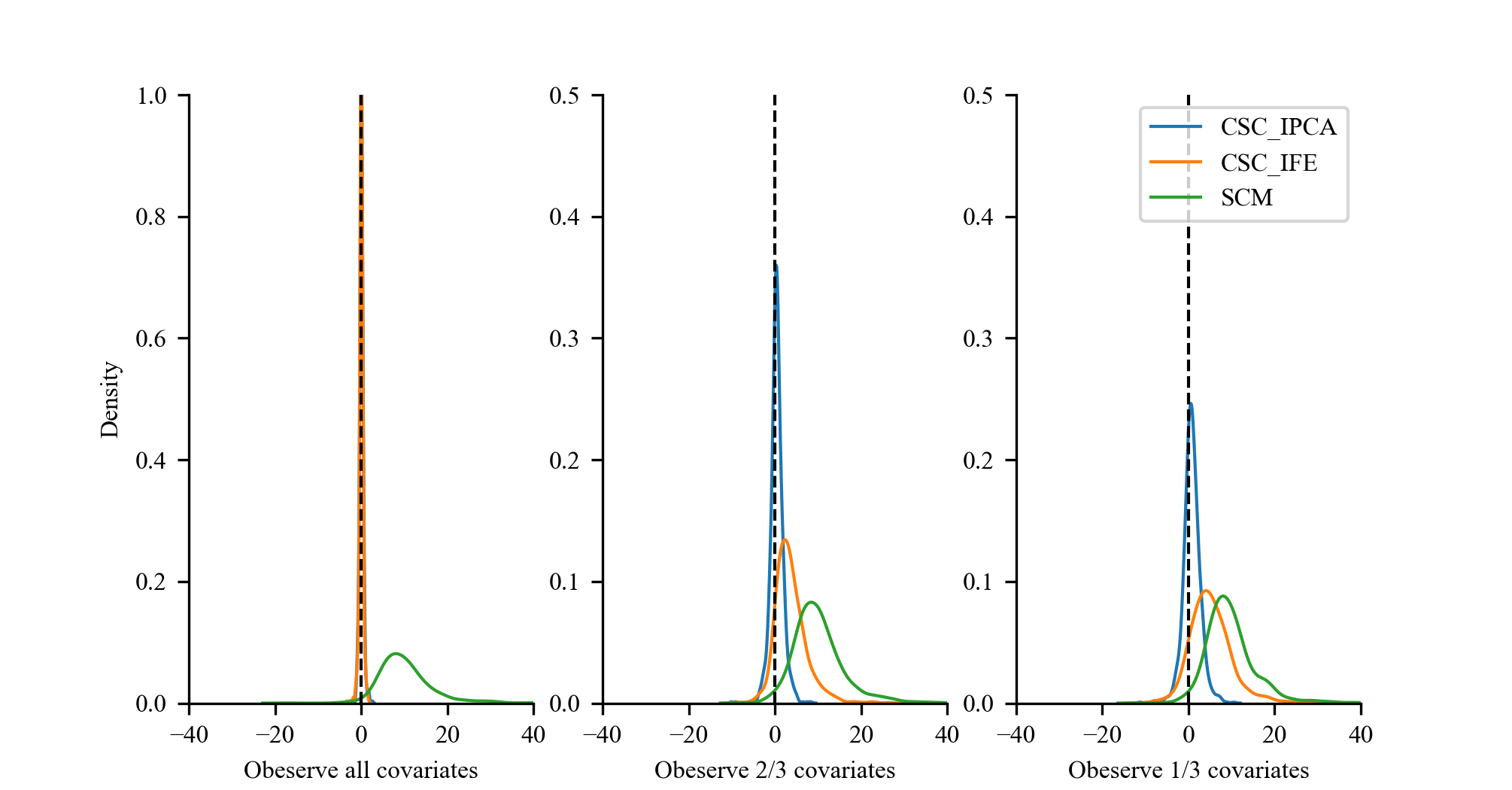
Figure 3: Bias Comparing with Other Methods

This graphic plots the bias of the CSC-IPCA, CSC-IFE, and SCM estimators for simulated data $N_{treat}=5,N_{ctrl}=45,T_{0}=20,T_{1}=10,L=10$.

4.3 Finite sample properties

We present the Monte Carlo simulation results in Table 1 to investigate the finite sample properties of the CSC-IPCA estimator. The numbers of treated units and post-treatment periods are fixed at $N_{treat}=5$ and $T_{post}=5$. We vary the number of control units $N_{ctrl}$, pre-treatment periods $T_{pre}$, and the proportion of observed covariates $\alpha$ with the total number of covariates $L=9$ to investigate the finite sample properties. As shown in Table 1, the bias, RMSE, and STD are estimated based on 1000 simulations. The results indicate that the bias of the CSC-IPCA estimator decreases as the number of control units and pre-treatment periods increases. As suggested by the theoretical results, the convergence rate of the CSC-IPCA estimator is the smaller one between $\mathcal{O}_{p}\left(\sqrt{N_{ctrl}}\right)$ and $\mathcal{O}_{p}\left(\sqrt{N_{treat}T_{pre}}\right)$. In this simulation example, since the smaller one is always $\mathcal{O}_{p}\left(\sqrt{N_{ctrl}}\right)$, we observe that the bias decreases significantly when the number of control units increases from 10 to 40. The number of observed covariates also plays a crucial role in bias reduction. The bias decreases the most when the proportion of observed covariates increases from $1/3$ to 1 (all covariates are observed). We observe a similar pattern in RMSE and STD. It is worth noting that if we observe all the covariates (i.e., $\alpha=1$), the bias, RMSE, and STD of the CSC-IPCA estimator all reduce to the lowest levels, even with a small number of control units and pre-treatment periods. We present the finite sample properties of the CSC-IFE and SCM estimators in Appendix C.2. When observing all the covariates, the CSC-IFE estimator is comparable to the CSC-IPCA estimator; however, when the number of observed covariates decreases, the CSC-IFE estimator becomes more biased than the CSC-IPCA estimator. The SCM estimator is always biased due to the settings.

Table 1: Finite Sample Properties

$\alpha$		$1/3$	$2/3$	1	$1/3$	$2/3$	1	$1/3$	$2/3$	1
$T_{0}$	$N_{ctrl}$	Bias			RMSE			STD
10	10	2.328	0.703	0.130	4.770	3.068	1.642	4.175	3.032	1.684
10	20	1.367	0.312	0.053	3.484	2.209	0.914	3.260	2.219	1.008
10	40	1.026	0.196	0.051	2.776	1.752	0.714	2.616	1.781	0.821
20	10	2.957	1.029	0.217	4.817	2.696	1.135	3.814	2.544	1.179
20	20	1.435	0.438	0.055	3.280	1.754	0.745	2.982	1.773	0.860
20	40	1.093	0.167	0.042	2.613	1.348	0.602	2.430	1.409	0.757
40	10	2.905	1.232	0.145	4.911	3.035	0.969	3.972	2.797	1.065
40	20	1.670	0.399	0.019	3.592	1.718	0.724	3.221	1.737	0.861
40	40	0.876	0.295	0.006	2.675	1.418	0.574	2.556	1.441	0.697

• This table presents the finite sample properties of the CSC-IPCA method estimated ATT for simulated data. The number of treated units and post-treatment period are fixed to $N_{treat}=5$ and $T_{1}=5$. We vary the number of control units $N_{ctrl}$, pre-treatment period $T_{0}$, and proportion of observed covariates $\alpha$ to investigate the finite sample properties, the total number of covariates is $L=9$. The bias, RMSE, and STD are estimated based on 1000 simulations.

5 Empirical Application

For the empirical application, we examine the impact of Brexit on foreign direct investment (FDI) in the United Kingdom (UK). The UK’s decision to leave the European Union (EU) has significantly influenced both its own economy, as discussed by Arnorsson and Zoega (2018), and the global economy, as detailed by Colantone and Stanig (2018). Historically, the UK has been a major recipient of FDI, with the EU being its largest source. The 2016 Brexit referendum introduced substantial uncertainty and volatility into the UK economy, directly affecting FDI. Although several studies, such as Dhingra et al. (2016) and Welfens and Baier (2018), have explored the impact of Brexit on FDI in the UK, they have not empirically examined this impact due to constraints in data and a lack of valid econometric methodology. In this paper, we aim to estimate the causal effect of Brexit on FDI to the UK using the CSC-IPCA method proposed herein.

The data used in this study is sourced from the World Development Indicators (WDI). The dataset includes information on FDI net inflows to the UK and other OECD countries, as well as other relevant variables such as GDP, imports and exports, inflation, investment, employment, and demographic indicators, the detailed description of the dataset is presented in the Appendix D.1. The dataset covers the period from 1995 to 2022, with the Brexit referendum taking place in 2016. We define the treatment period as the post-Brexit period, starting from 2017, and the pre-treatment period as the period from 1995 to 2016. The treated unit is the UK, while the control units are the rest of the OECD countries.

One of the key challenges in estimating the impact of Brexit on FDI is the high volatility of FDI data. As shown in Figure D.5, FDI net inflows to each country can fluctuate significantly from year to year, making it difficult to identify the causal effect of specific events, such as Brexit. The conventional DID method may not be suitable for this type of data, as it requires the parallel trend assumption to hold, which is unlikely in this case. The synthetic control method may also fail to provide an unbiased estimate due to the high volatility of the FDI data on the one hand. On the other hand, since the treated unit is the UK, a global financial center with significant foreign investment, the FDI to GDP ratio may fall outside the convex hull of the control units, which are predominantly conventional OECD countries with less FDI compared to an international financial center like the UK. The novel CSC-IFE method is suitable for this type of data, as it can handle high volatility, lack of common support, and non-parallel trends. However, there are still caveats with the CSC-IFE method. The first concern is whether we have the correct model specification for the DGPs, since the CSC-IFE method relies on a factor model. The second concern is the high dimensionality of the covariates, as many variables seem to be relevant to FDI. Lastly, there is the issue of omitted variable bias; given the limited research on country-level FDI, there might be important variables that are not yet measured or observed. The CSC-IPCA method can address these issues by providing a more flexible and robust estimation of the causal effect of Brexit on FDI in the UK, as discussed in the previous sections with our simulations.

For simplicity, we choose the number of latent factors $K=2$ instead of performing hyperparameter tuning. The model converges after 52 iterations, and the estimated ATT is presented in Figure 4. The upper panel of the figure shows the actual FDI net inflows to the UK and the postulated ones for the entire time period. We observe that before 2017, the postulated FDI net inflows to the UK are very close to the actual FDI net inflows, indicating that the CSC-IPCA method effectively captures the trend in FDI net inflows to the UK. However, after 2017, the postulated counterfactual FDI net inflows to the UK diverge from the actual values.

The lower panel of the figure shows the estimated ATT with the 90% confidence interval based on conformal inference. The estimated ATT is -7.8% in 2017, -12.9% in the following year, and -18.3% in 2019. The confidence intervals for these three years are all negative, providing strong evidence that Brexit has a negative impact on FDI net inflows to the UK. However, after 2019, the confidence intervals become wide and less reliable. One possible reason is that the FDI data is highly volatile and has been deteriorated by the COVID-19 pandemic globally.

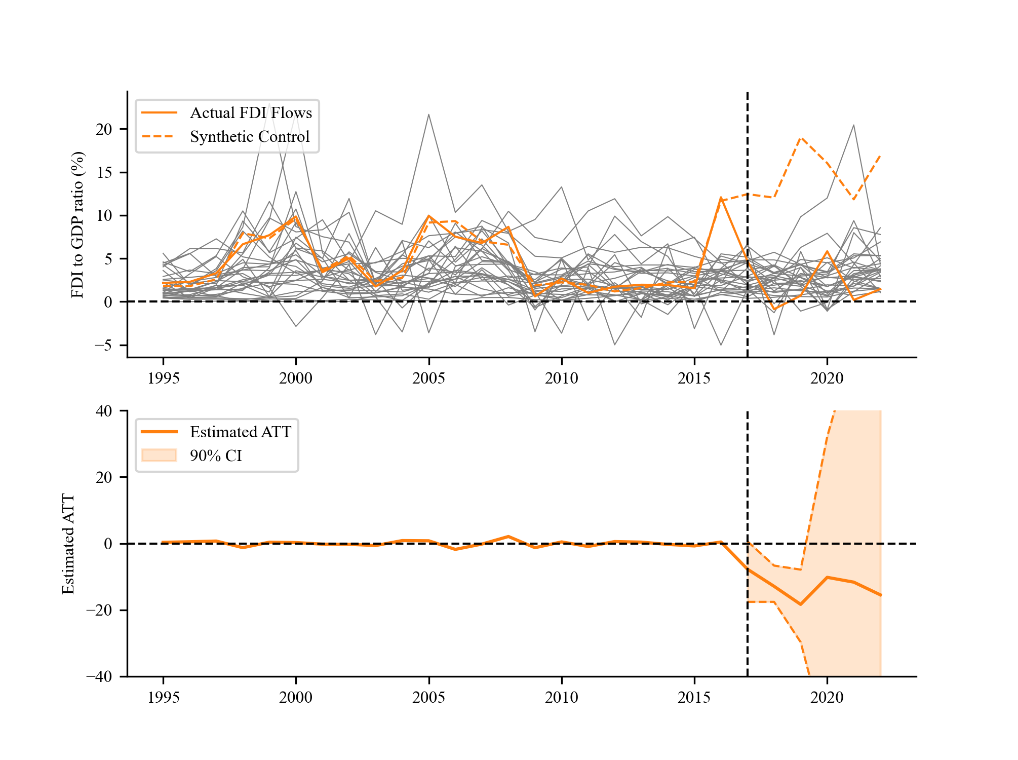
Figure 4: CSC-IPCA Estimated ATT for Brexit

This graphic plots the CSC-IPCA method estimated ATT for the impact of Brexit on FDI in the UK.

The CSC-IPCA method estimates the common factors and factor loadings for the FDI data. The two estimated common factors, presented in Figure 5, are orthogonal to each other. The first common factor is more volatile, capturing the peak before the dot-com bubble burst in the late 1990s, the downturn following the bubble burst in the 2000s, and the Global Financial Crisis in 2008. The second common factor is more stable, though its interpretation is less clear. The lower panel of the figure displays the factor loadings for the UK, highlighting the time dynamics of the UK’s FDI net inflows—a key difference from conventional factor models, which assume constant factor loadings over time. The first factor loading is more stable, and when it interacts with the first common factor, the interaction term primarily captures the global economic cycle’s impact on FDI net inflows to the UK. In contrast, the second factor loading is more volatile, and its interaction with the second common factor captures idiosyncratic shocks to the UK’s FDI net inflows.

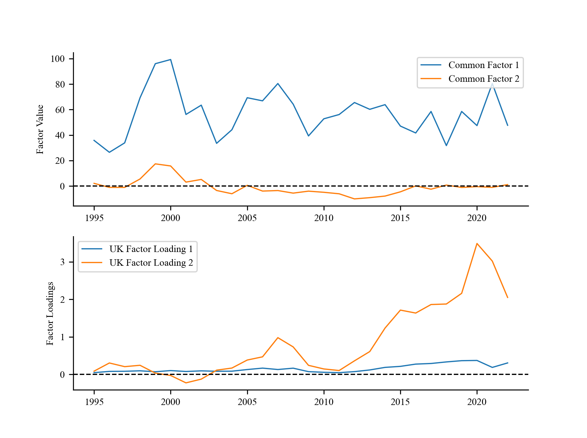
Figure 5: Estimated Common Factors

This graphic plots the estimated common factors for FDI in OECD countries.

To further illustrate the time-varying factor loadings, we present the factor loadings for selected countries in Figure 6. Most countries exhibit similar patterns in the relative magnitudes of the two factor loadings. We observe that the second factor loading for the US forms an approximate V-shape before and after the 2008 Global Financial Crisis, indicating a strong inflow of FDI after the crisis. The first factor loading for the US is relatively stable, similar to that of the UK. The factor loadings for Germany and France are similar, reflecting their geographic and political proximity. Japan’s factor loadings display a different pattern, particularly in the second factor loading, which represents idiosyncratic shocks to Japan’s FDI inflows, reflecting the prolonged struggles of the Japanese economy since the crash of the real estate bubble in the 1990s.

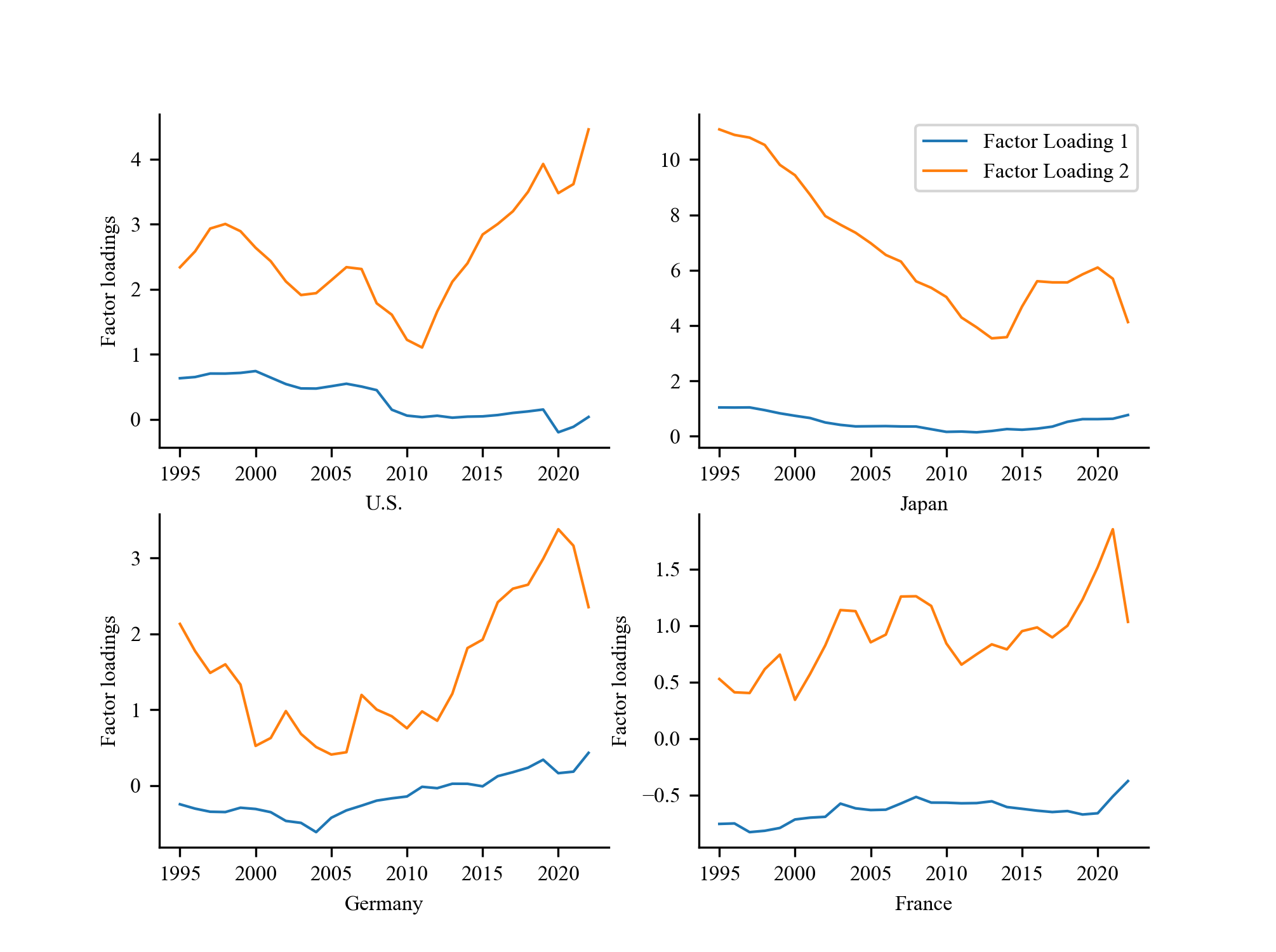
Figure 6: Factor Loadings of Selected Countries

This graphic plots the factor loadings of selected countries.

6 Conclusion

In this paper, we propose a new causal inference method for estimating the ATT. This method belongs to the wide family of counterfactual and synthetic control methods, and is based on the novel generalized synthetic control method (i.e. CSC-IFE method in this paper.), to impute the counterfactual by modeling the whole data generating processes.

The proposed method, CSC-IPCA, pushes the frontier of the CSC-IFE method in three aspects. First, the CSC-IPCA method can easily handle high-dimensional covariates, as it employs the dimension reduction process through the mapping matrix $\Gamma$. Second, the CSC-IPCA method can capture the time-varying factor loadings, as it instruments the factor loadings with the covariates. Importantly the dynamic factor loadings have better economic interpretation and can help to better estimate the common factors. Third, it does not require the correct model specification for the DGPs because of the way how it incorporates the covariates.

Through Monte Carlo simulations, we demonstrate that the CSC-IPCA method outperforms the CSC-IFE method, particularly in the presence of omitted variables. Our formal results and finite sample properties show that the CSC-IPCA estimator is consistent and converges rapidly to the true ATT, depending on the smaller of the number of control units or the number of pre-treatment periods. In the empirical application, we use the CSC-IPCA method to estimate the impact of Brexit on FDI in the UK. The results indicate that Brexit has a negative impact on FDI net inflows. The confidence intervals based on conformal inference are all negative before the COVID-19 pandemic, providing strong evidence to support our estimates.

One limitation of the CSC-IPCA method is the risk of overfitting when the number of latent factors or covariates is too large. While we provide two methods for selecting the number of latent factors, we suggest starting with 1 or 2 factors and increasing the number only if the initial results are unsatisfactory. Another concern is the potential contamination from bad controls, which we do not address in this paper. For future research, there are two key directions: first, improving techniques to manage overfitting; and second, exploring ways to address the issue of bad controls, with the goal of developing a “kitchen sink” model that can effectively incorporate all covariates—both good and bad—without compromising the integrity of the analysis.

Appendix A Technical Details

A.1 Treatment Assignment

To simplify the computation, we assume that the treatment assignment is based on a block assignment mechanism.

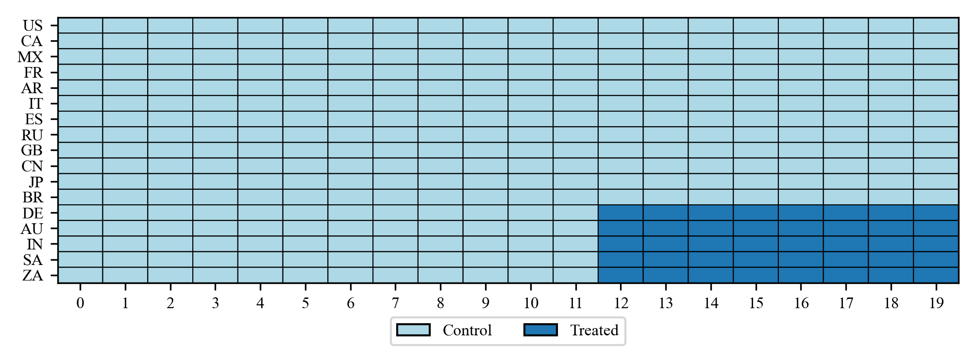
Figure A.1: Block Assignment

This graphic depicts the block assignment mechanism. Control units remain untreated throughout, while treated units receive the intervention simultaneously. Once the treatment is initiated, it is maintained permanently and cannot be reversed.

The CSC-IPCA method can also be applied to estimate the staggered adoption mechanism, where treated units receive the intervention at different time points. The most complex scenario is the random assignment, where the treatment assignment is random and can be switched on or off at any time. This topic is beyond the scope of this paper, but matrix completion with nuclear norm, as detailed in Athey et al. (2021), is a suitable approach for such cases.

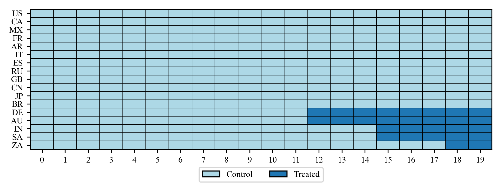
Figure A.2: Staggered Adoption

This graphic presents the staggered adoption mechanism. Control units remain untreated throughout, while treated units receive the intervention at different time points. Once the treatment is initiated, it is maintained permanently and cannot be reversed.

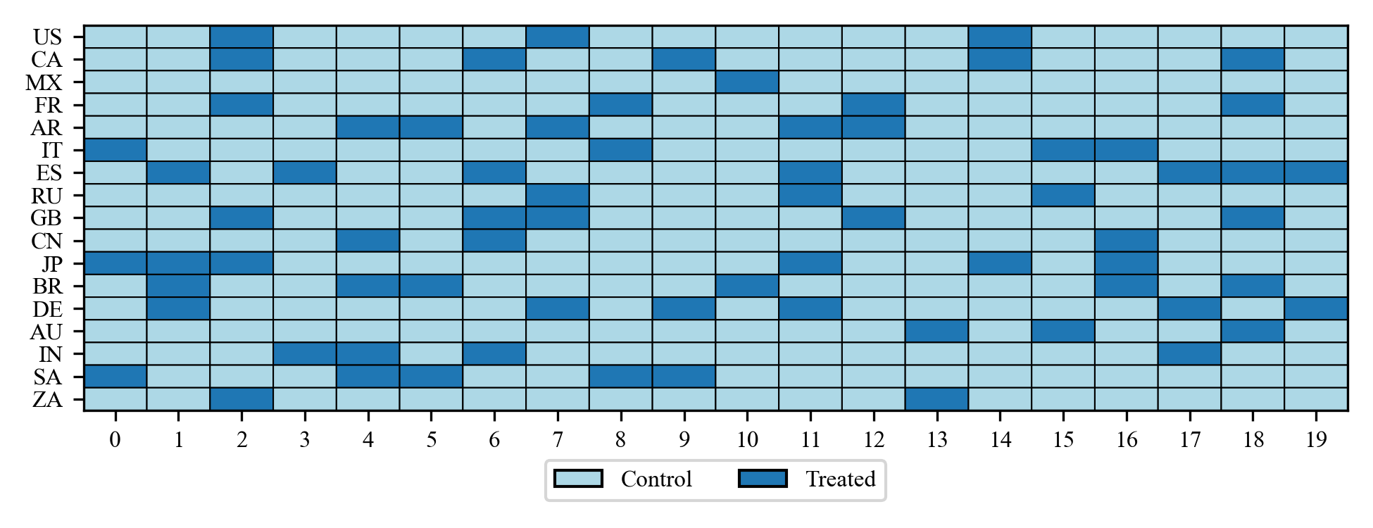
Figure A.3: Random Assignment

This graphic illustrates the random assignment mechanism. All units are randomly assigned to either the control or treatment group. The treatment can be switched on or off at any time.

A.2 Identification assumptions

Following this section, we use lowercase letters to represent scalars, e.g., $y_{it}$ would be a scalar of the outcome variable for unit $i$ at time $t$. We use bold lowercase letters to represent vectors, e.g., $\bm{x}_{it}$ would be a vector of covariates for unit $i$ at time $t$. We use uppercase letters to represent matrices, e.g., $\Gamma$ represents the mapping matrix. We denote $\mathbb{E}\|\bm{f}_{t}\bm{f}_{t}^{\prime}\|^{2}$ the Frobenius norm squared of the matrix $\bm{f}_{t}\bm{f}^{\prime}_{t}$.

Assumption A.2

Assumption for consistency:

1. Covariate orthogonality: $\mathbb{E}\left[\textbf{x}^{\prime}_{it}\epsilon_{it}\right]=\textbf{0}_{L\times 1}$,

2. The following moments exist: $\mathbb{E}\|\bm{f}_{t}\bm{f}^{\prime}_{t}\|^{2}$, $\mathbb{E}\|\bm{x}^{\prime}_{it}\epsilon_{it}\|^{2}$, $\mathbb{E}\|\bm{x}^{\prime}_{it}\bm{x}_{it}\|^{2}$, $\mathbb{E}\left[\|\bm{x}^{\prime}_{it}\bm{x}_{it}\|^{2}\|\bm{f}_{t}\bm{f}^{\prime}_{t}\|^{2}\right]$,

3. Almost surely, $\bm{x}_{it}$ is bounded, and define $\Omega_{t}^{xx}:=\mathbb{E}\left[\bm{x}_{it}^{\prime}\bm{x}_{it}\right]$, then almost surely, $\Omega_{t}^{xx}>\epsilon$ for some $\epsilon>0$.

4. The parameter space $\Psi$ of $\Gamma$ is compact and away from rank deficient: $\det{\Gamma^{\prime}\Gamma}>\epsilon$ for some $\epsilon>0$,

Assumption A.3

Assumptions for asymptotic normality:

1. $\text{As }N,T\to\infty,\>\frac{1}{\sqrt{NT}}\sum_{i,t}\text{vect}\left(\bm{x}^{\prime}_{i,t}\epsilon_{i,t}\bm{f}^{\prime}_{t}\right)\xrightarrow{d}\text{Normal}\left(0,\Omega^{x\epsilon f}\right)$,

2. $\text{As }N\to\infty,\>\frac{1}{\sqrt{N}}\sum_{i}\text{vect}\left(X^{\prime}_{i}\epsilon_{i}\right)\xrightarrow{d}\text{Normal}\left(0,\Omega^{x\epsilon}\right)\>\text{for}\>\forall t$,

3. $\text{As }N,T\to\infty,\>\frac{1}{\sqrt{T}}\sum_{t}\text{vect}\left(\bm{f}_{t}\bm{f}^{\prime}_{t}-\mathbb{E}[\bm{f}_{t}\bm{f}^{\prime}_{t}]\right)\xrightarrow{d}\text{Normal}\left(0,\Omega^{f}\right)$.

4. Bounded dependence: $\frac{1}{NT}\sum_{i,j,t,s}\|\tau_{ij,ts}\|<\infty$, where $\tau_{ij,ts}:=\mathbb{E}\left[\bm{x}^{\prime}_{it}\epsilon_{it}\epsilon^{\prime}_{js}\bm{x}_{js}\right]$

5. Constant second moments of the covariates: $\Omega_{t}^{xx}=\mathbb{E}\left[X_{t}X^{\prime}_{t}\right]$ is constant across time periods.

A.3 Estimation of the CSC-IPCA estimator

As outlined in Equation 3, the structural components of the data generating process are constructed by the interactive fixed effect between time-varying factors $\bm{f}_{t}$ and dynamic factor loadings $\bm{\lambda}_{it}$, which is instrumented by the covariates $\bm{x}_{it}$ through the mapping matrix $\Gamma$. The data generating process can be formulated as follows:

$$y_{it}=(\bm{x}_{it}\Gamma)\bm{f}^{\prime}_{t}+\epsilon_{it},\quad\epsilon_{it}=\mu_{it}+\bm{h}_{it}\bm{f}^{\prime}_{t}.$$ (A.1)

where the error term $\epsilon_{it}$ is combined with the interaction between time-varying factors $\bm{f}_{t}$ and error term associated with factor loadings $\bm{h}_{it}$ and the idiosyncratic error $\mu_{it}$. The objective function in Equation 6 is minimized to estimate the factor $\bm{f}_{t}$ and mapping matrix $\Gamma$. Equation A.2 details the first step to estimate the factor $\bm{f}_{t}$ and mapping matrix $\Gamma$ with only the control units:

$$(\hat{\Gamma}_{ctrl},\hat{\bm{f}}_{t})=\underset{\Gamma,\bm{f}_{t}}{\arg\min}\sum_{i\in\mathcal{T}}\sum_{t\leq T}\left(y_{it}-(\bm{x}_{it}\Gamma)\bm{f}^{\prime}_{t}\right)^{\prime}\left(y_{it}-(\bm{x}_{it}\Gamma)\bm{f}^{\prime}_{t}\right).$$ (A.2)

The alternating least squares (ALS) method is employed for the numerical solution of this optimization problem. Unlike PCA, the IPCA optimization challenge cannot be resolved through eigen decomposition. The optimization, as defined in the equation above, is quadratic with respect to either $\Gamma$ or $\bm{f}_{t}$, when the other is held constant. This characteristic permits the analytical optimization of $\Gamma$ and $\bm{f}_{t}$ sequentially. With a fixed $\Gamma$, the solutions for $\bm{f}_{t}$ are t-separable and can be obtained via cross-sectional OLS for each $t$:

$$\hat{\bm{f}}_{t}(\Gamma)=(\Gamma^{\prime}\bm{x}^{\prime}_{t}\bm{x}_{t}\Gamma)^{-1}\Gamma^{\prime}\bm{x}^{\prime}_{t}y_{t}.$$ (A.3)

Conversely, with known $\bm{f}_{t}$, the optimal $\Gamma$ (vectorized as $\bm{\gamma}=vect(\Gamma)$) is derived through pooled OLS of $y_{it}$ against $LK$ regressors, $\bm{x}_{it}\otimes\bm{f}_{t}$:

$$\hat{\gamma}=\left(\sum_{i,t}(\bm{x}_{i,t}^{\prime}\otimes\bm{f}_{t})(\bm{x}_{i,t}\otimes\bm{f}_{t}^{\prime})\right)^{-1}\left(\sum_{i,t}(\bm{x}_{i,t}^{\prime}\otimes\bm{f}_{t})y_{i,t}\right).$$ (A.4)

Inspired by PCA, the initial guess for $\bm{f}_{t}$ is the first $K$ principal components of the $N\times T$ outcome matrix $Y$. The ALS algorithm alternates between these two steps until convergence is achieved, typically reaching a local minimum rapidly. The convergence criterion, based on the minimization of relative change in the parameters $\bm{f}_{t}$ and $\Gamma$ in each iteration, ensures termination when this change falls below a predefined threshold, set at $1e-6$ in our implementation.

As we have mentioned before the estimation of $\bm{f}_{t}$ and $\Gamma$ is not deterministic. Bai (2009) and Xu (2017) set the constraints on the factor loadings and factors before the estimation to ensure the identifiability of the model. However, in our case, since the structural component is identified by the product between factors and factor loadings $\bm{x}_{it}\Gamma\bm{f}^{\prime}_{t}$, we can find any arbitrary rotation matrix $R$, such that $\bm{x}_{it}\Gamma RR^{-1}\bm{f}^{\prime}_{t}$ yields the same structural component. For a specific constraints on the mapping matrix $\Gamma_{norm}=\Gamma_{treat}R$ and factor $\bm{f}_{norm}=R^{-1}\bm{f}_{t}$, such that:

$$\Gamma_{norm}^{\prime}\Gamma_{norm}=\mathcal{I}_{K},$$ (A.5)

$$\bm{f}_{norm}\bm{f}_{norm}^{\prime}/T=\text{Diagonal}.$$

where $\mathcal{I}_{K}$ is a $K\times K$ identity matrix, and $T$ is the number of time periods. The rotation matrix $R$ can be easily found by the following steps: first, we use Cholesky decomposition (referred to Higham (2009) for a guidence) to decompose the product $\Gamma^{\prime}\Gamma$ into an upper triangular matrix $R_{1}=cholesky(\Gamma^{\prime}\Gamma)$, then we perform singular value decomposition on $R_{1}\bm{f}_{t}\bm{f}_{t}^{\prime}R_{1}^{\prime}$ to get $R_{2}=U$ where $U\Sigma V^{\prime}=svd(R_{1}\bm{f}_{t}\bm{f}_{t}^{\prime}R_{1}^{\prime})$. Finally, the rotation matrix $R$ is given by:

$$R=R_{1}^{-1}R_{2}.$$ (A.6)

A.4 Hyperparameter tuning

We can also utilize leave-one-out cross-validation to select the hyperparameter $K$, as detailed in Algorithm 2. This method involves excluding the $t^{th}$ period data from the control group to serve as the training data, while similarly excluding the corresponding period data from the treated group to act as validation data. This process is repeated for each time period in the pretreatment phase, applying a predetermined number of factor loadings. The optimal number of factors, $K$, is identified as the one that yields the minimum average of sum squared errors across all iterations.

Data: $Y,X$

Result: Optimal hyperparameter $k$

1 Determine the maximum possible hyperparameter $K$;

2 Initialize an array $MSE$ to store the average of sum squared error for each $k$;

3 for $k=1$ to $K$ do

4       Set sum of squared errors $SSE_{k}=0$;

5       for $t\leftarrow 1$ to $T_{pre}$ do

6             Remove the $t^{th}$ period observation from control data, using the rest as training data $(Y_{ctrl}^{-t},X_{ctrl}^{-t})$;

7            

8            Similarly, exclude the $t^{th}$ period observation from treated data, using the rest as validation data $(Y_{treat}^{-t},X_{treat}^{-t})$;

9            

10            Estimate parameters $\Gamma$ and $F_{t}$ using the training data via the ALS method;

11            

12            Use the estimated $\hat{\Gamma}$ and $\hat{F}_{t}$ to predict $\hat{Y}^{-t}_{treat}$ with the validation data;

13            

14            Calculate the sum squared error $SE_{t}=\sum(Y_{treat}^{-t}-\hat{Y}_{treat}^{-t})^{2}$;

15            

16            Accumulate the sum of squared errors: $SSE_{k}\leftarrow SSE_{k}+SE_{t}$;

17            

18       end for

19      Calculate the average sum squared error for $k$: $MSE[k]=\frac{SSE_{k}}{T_{pre}}$;

20      

21 end for

22Select $k$ corresponding to the minimum value in $MSE$;

Algorithm 2 Leave-One-Out Cross-Validation for Hyperparameter $k$

Appendix B Formal Result

In this section, we derive the formal result for the CSC-IPCA estimator. We first establish the consistency and asymptotic properties of the mapping matrix $\Gamma$ and the factor $\bm{f}_{t}$. We then derive the formal result for the CSC-IPCA estimated ATT.

B.1 Mapping matrix estimation asympototic properties

In this section, we delve into the asymptotic properties of the estimation error associated with the mapping matrix. Kelly et al. (2020) have proven it in their paper, referring to Theorem 3. The following proposition 1, is a special case of their result. Based on our estimation methods, we estimate the mapping matrix $\Gamma$ first by concentrating out the factor $\bm{f}_{t}$, as shown in Equation 6, we can formulate a target function for $\Gamma$ as follows:

$$G(\Gamma)=\frac{1}{2NT}\sum_{i,t}\left(y_{it}-\bm{x}_{it}\Gamma\bm{\hat{f}}_{t}\right)^{2}.$$ (B.7)

we define the score function $S(\Gamma)$ as the derivative of the target function $G(\Gamma)$ with respect to $\Gamma$: $S(\Gamma)=\frac{\partial G(\Gamma)}{\partial\Gamma}$. The Hessian matrix $H(\Gamma)$ is defined as the second derivative of the target function $G(\Gamma)$ with respect to $\Gamma$: $H(\Gamma)=\frac{\partial^{2}G(\Gamma)}{\partial\Gamma\partial\Gamma^{\prime}}$.

It is crucial to highlight that our normalization criterion, delineated in Equation 9, mandates that the mapping matrix $\Gamma$ adheres to orthonormality and the factor $\bm{f}_{t}\bm{f}_{t}^{\prime}/T$ is required to exhibit orthogonality. To satisfy these requirements we define the following identification function:

$$I(\Gamma):=\begin{bmatrix}\text{veca}(\Gamma^{\prime}\Gamma-\mathcal{I}_{K})\\ \text{vecb}\left(\frac{1}{T}\sum_{t}\bm{\hat{f}}_{t}\bm{\hat{f}}_{t}^{\prime}-V^{ff}\right)\end{bmatrix}$$ (B.8)

where $V^{ff}=E\left[\bm{f}_{t}\bm{f}^{\prime}_{t}\right]$, meanwhile, $\text{veca}(\cdot)$ and $\text{vecb}(\cdot)$ vectorize the upper triangular entries of a square matrix. The difference is $\text{veca}(\cdot)$ includes the diagonal elements, while $\text{vecb}(\cdot)$ excludes them. We define the Jacobian matrix $J(\Gamma)$ as the derivative of the identification function $I(\Gamma)$ with respect to $\Gamma$: $J(\Gamma)=\frac{\partial I(\Gamma)}{\partial\Gamma}$.

Proposition 1

Under Assumption A.2 and A.3, mapping matrix estimation error centered against the normalized true mapping matrix converges to a normal distribution at the rate of $\sqrt{NT}$: as $N,T\rightarrow\infty$ such that $T/N\rightarrow\infty$,

$$\sqrt{NT}\left(\hat{\bm{\gamma}}-\bm{\gamma}^{0}\right)\xrightarrow{d}-\left(H^{0^{\prime}}H^{0}+J^{0^{\prime}}J^{0}\right)^{-1}H^{0^{\prime}}Normal(0,\mathbb{V}^{[1]})$$

where $H^{0}:=\frac{\partial^{2}G(\Gamma)}{\partial\bm{\gamma}\partial\bm{\gamma}^{\prime}}|_{\bm{\gamma}=\bm{\gamma}^{0}}$ and $J^{0}:=\frac{\partial I(\Gamma)}{\partial\bm{\gamma}}|_{\bm{\gamma}=\bm{\gamma}^{0}}$, $\mathbb{V}^{[1]}=\left(Q^{0}\otimes\mathcal{I}_{K}\right)\Omega^{x\epsilon f}\left(Q^{0^{\prime}}\otimes\mathcal{I}_{K}\right)$, and $Q^{0}:=Q_{t}(\Gamma^{0})$ given that $Q_{t}(\Gamma):=\mathcal{I}_{L}-\Omega_{t}^{xx}\left(\Gamma^{\prime}\Omega^{xx}_{t}\Gamma\right)^{-1}\Gamma^{\prime}$ is constant over $t$ under Assumption A.3.

Proof: referring to Kelly et al. (2020).

B.2 Factor estimation asympototic properties

Proposition 2

Under Assumption A.2 and A.3, factor estimation error centered against the normalized true factor converges to a normal distribution at the rate of $\sqrt{N}$: as $N,T\to\infty$ for $\forall t$,

$$\sqrt{N}\left(\hat{\bm{f}}_{t}-\bm{f}^{0}_{t}\right)\xrightarrow{d}N\left(0,\mathbb{V}_{t}^{[2]}\right),$$

where the variance term $\mathbb{V}_{t}^{[2]}$, which is given by $\mathbb{V}_{t}^{[2]}=\left(\Gamma^{\top}\Omega_{t}^{xx}\Gamma\right)^{-1}\Gamma^{\top}\Omega_{t}^{x\epsilon}\Gamma\left(\Gamma^{\top}\Omega_{t}^{xx}\Gamma\right)^{-1}$.

Proof: Decompose the left-hand side equation:

$$\sqrt{N}\left(\bm{\hat{f}}_{t}-\bm{f}_{t}\right) =\sqrt{N}\left(\left(\hat{\Gamma}^{\prime}X^{\prime}_{t}X_{t}\hat{\Gamma}\right)^{-1}\hat{\Gamma}^{\prime}X_{t}^{\prime}\left(X_{t}\hat{\Gamma}\bm{f}_{t}+\bm{\tilde{\epsilon}}_{t}\right)-\bm{f}_{t}\right)$$

$$=\sqrt{N}\left(\left(\hat{\Gamma}^{\prime}X^{\prime}_{t}X_{t}\hat{\Gamma}\right)^{-1}\hat{\Gamma}^{\prime}X_{t}^{\prime}\left(X_{t}\hat{\Gamma}\bm{f}_{t}\right)-\bm{f}_{t}\right)+\sqrt{N}\left(\hat{\Gamma}^{\prime}X^{\prime}_{t}X_{t}\hat{\Gamma}\right)^{-1}\hat{\Gamma}^{\prime}X_{t}^{\prime}\bm{\tilde{\epsilon}}_{t}$$

where $\bm{\tilde{\epsilon}}_{t}$ is the estimated error term with estimated $\hat{\Gamma}$ and true $\bm{f}_{t}$. Given Proposition 1, $\hat{\Gamma}-\hat{\Gamma}^{0}=\mathcal{O}_{p}\left(1/\sqrt{NT}\right)$. The first term is simply $\mathcal{O}_{p}\left(1/\sqrt{NT}\right)$. For the second term:

$$\sqrt{N}\left(\hat{\Gamma}^{\prime}X^{\prime}_{t}X_{t}\hat{\Gamma}\right)^{-1}\hat{\Gamma}^{\prime}X_{t}^{\prime}\bm{\tilde{\epsilon}}_{t}= \sqrt{N}\left(\Gamma^{\prime}X^{\prime}_{t}X_{t}\Gamma\right)^{-1}\Gamma^{\prime}X_{t}^{\prime}\bm{\epsilon_{t}}+\mathcal{O}_{p}(1)$$

$$\xrightarrow{d}Normal(0,\mathbb{V}_{t}^{[2]})$$

Assumption A.3 delineates the properties of $\Omega_{t}^{xx}$ and $\Omega_{t}^{x\epsilon}$. Notably, despite the presence of multiple matrix multiplications, the matrices $\Omega_{t}^{xx}$ and $\Omega_{t}^{x\epsilon}$ remain invariant under these operations. Consequently, the term $\mathbb{V}_{t}^{[2]}$ is constant across all observational units.

B.3 Consistency and asymptotic property of the ATT estimation

Theorem 1

Under Assumptions 1, A.2, and A.3, the CSC-IPCA estimator $\mathbb{E}\left(\widehat{ATT}_{t}|D,X,\Gamma,F\right)\xrightarrow{P}ATT_{t}$, where $ATT_{t}=\frac{1}{N_{treat}}\sum_{i\in\mathcal{T}}\delta_{it}$ is the true treatment effect. for all $t>T_{pre}$ as both $N_{ctrl},\ T_{pre}\to\infty$.

Proof: Denote $i$ as the treated unit on which the treatment effect is of interest, the bias of estimated ATT is given by:

$$\hat{\delta}_{it}-\delta_{it} =y_{it}^{1}-\hat{y}_{it}^{0}-\delta_{it},$$

$$=\textbf{x}_{it}\Gamma\bm{f}^{\prime}_{t}-\textbf{x}_{it}\hat{\Gamma}\hat{\bm{f}}^{\prime}_{t}+\epsilon_{it},$$

$$=\textbf{x}_{it}\left(\left(\mathcal{I}_{L}\otimes\bm{f}_{t}\right)\bm{\gamma}-(\mathcal{I}_{L}\otimes\hat{\bm{f}}_{t})\hat{\bm{\gamma}}\right)+\epsilon_{it},$$

$$=\textbf{x}_{it}\left(\left(\mathcal{I}_{L}\otimes\bm{f}_{t}\right)\bm{\gamma}-\mathcal{I}_{L}\otimes(\bm{f}_{t}+\bm{e}_{f_{t}})(\bm{\gamma}+\textbf{e}_{\gamma})\right)+\epsilon_{it},$$

$$=\textbf{x}_{it}\left((\mathcal{I}_{L}\otimes\bm{f}_{t})\textbf{e}_{\gamma}-(\mathcal{I}_{L}\otimes\bm{e}_{f_{t}}\bm{\gamma})-(\mathcal{I}_{L}\otimes\bm{e}_{f_{t}})\textbf{e}_{\gamma}\right)+\epsilon_{it}$$

$$=\textbf{x}_{it}E_{\Gamma}\bm{f}^{\prime}_{t}-\textbf{x}_{it}\Gamma\bm{e}^{\prime}_{f_{t}}-\textbf{x}_{it}E_{\Gamma}\bm{e}^{\prime}_{f_{t}}+\epsilon_{it},$$

$$=A_{1,it}+A_{2,it}+A_{3,it}+\epsilon_{it}.$$

where $\bm{e}_{f_{t}}=\bm{f}_{t}-\hat{\bm{f}}_{t}$ is a vector of estimation error of the factor $\bm{f}_{t}$, $\bm{e}_{\gamma}$ is vectorized estimation error of the mapping matrix $E_{\Gamma}=\Gamma-\hat{\Gamma}$. The third step converts the vector-matrix multiplication into vector multiplications with the Kronecker product, $\bm{x}_{it}\Gamma\bm{f}^{\prime}_{t}=\bm{x}_{it}(\mathcal{I}_{L}\otimes\bm{f}_{t})\bm{\gamma}$, where $\mathcal{I}_{L}$ is an $L\times L$ identity matrix. The bias of the estimated ATT is the sum of four terms $A_{1,it}$, $A_{2,it}$, $A_{3,it}$, and $\epsilon_{it}$. By proposition 1 and 2, we have the following results:

$$A_{1,it}=\bm{x}_{it}E_{\Gamma}\bm{f}^{\prime}_{t}=\mathcal{O}_{p}\left(1/\sqrt{N_{treat}T_{pre}}\right).$$

$$A_{2,it}=-\bm{x}_{it}\Gamma\bm{e}^{\prime}_{f_{t}}=\mathcal{O}_{p}\left(1/\sqrt{N_{ctrl}}\right).$$

$$A_{3,it}=-\bm{x}_{it}E_{\Gamma}\bm{e}^{\prime}_{f_{t}}=\mathcal{O}_{p}\left(1/\sqrt{N_{treat}T_{pre}}\right).$$

Since we estimate the factor $\bm{f}_{t}$ using only control units and update the mapping matrix $\Gamma$ with treated units in the pre-treatment period, both $\bm{f}_{t}$ and $\Gamma$ converge over different dimensions of $T$ and $N$. Consequently, the error term $\epsilon_{it}$ is assumed to have zero means, leading to the bias of the estimated ATT also converging to zero:

$$\hat{\delta}_{it}-\delta_{it} =\mathcal{O}_{p}\left(\frac{1}{\sqrt{N_{treat}T_{pre}}}\right)+\mathcal{O}_{p}\left(\frac{1}{\sqrt{N_{ctrl}}}\right)+\mathcal{O}_{p}\left(\frac{1}{\sqrt{N_{treat}T_{pre}}}\right)+\epsilon_{it}$$

$$=\mathcal{O}_{p}\left(\frac{1}{\sqrt{N_{ctrl}}}\right)+\mathcal{O}_{p}\left(\frac{1}{\sqrt{N_{treat}T_{pre}}}\right).$$

Therefore, as $N_{\text{ctrl}},\ T_{\text{pre}}\to\infty$, the estimated ATT converges to the true ATT:

$$\mathbb{E}\left(\widehat{ATT}_{t}|D,X,\Gamma,F\right)\xrightarrow{P}ATT_{t}.$$

The convergence rate is the smaller one between $1/\sqrt{N_{ctrl}}$ and $1/\sqrt{N_{treat}T_{pre}}$.

Appendix C Simulation Study

C.1 Bias comparison with different DGPs

In this section, we provide additional simulation results to compare the bias of the CSC-IPCA, CSC-IFE, and SCM estimators with different data generating processes. We consider the data generating processes used in Xu (2017).

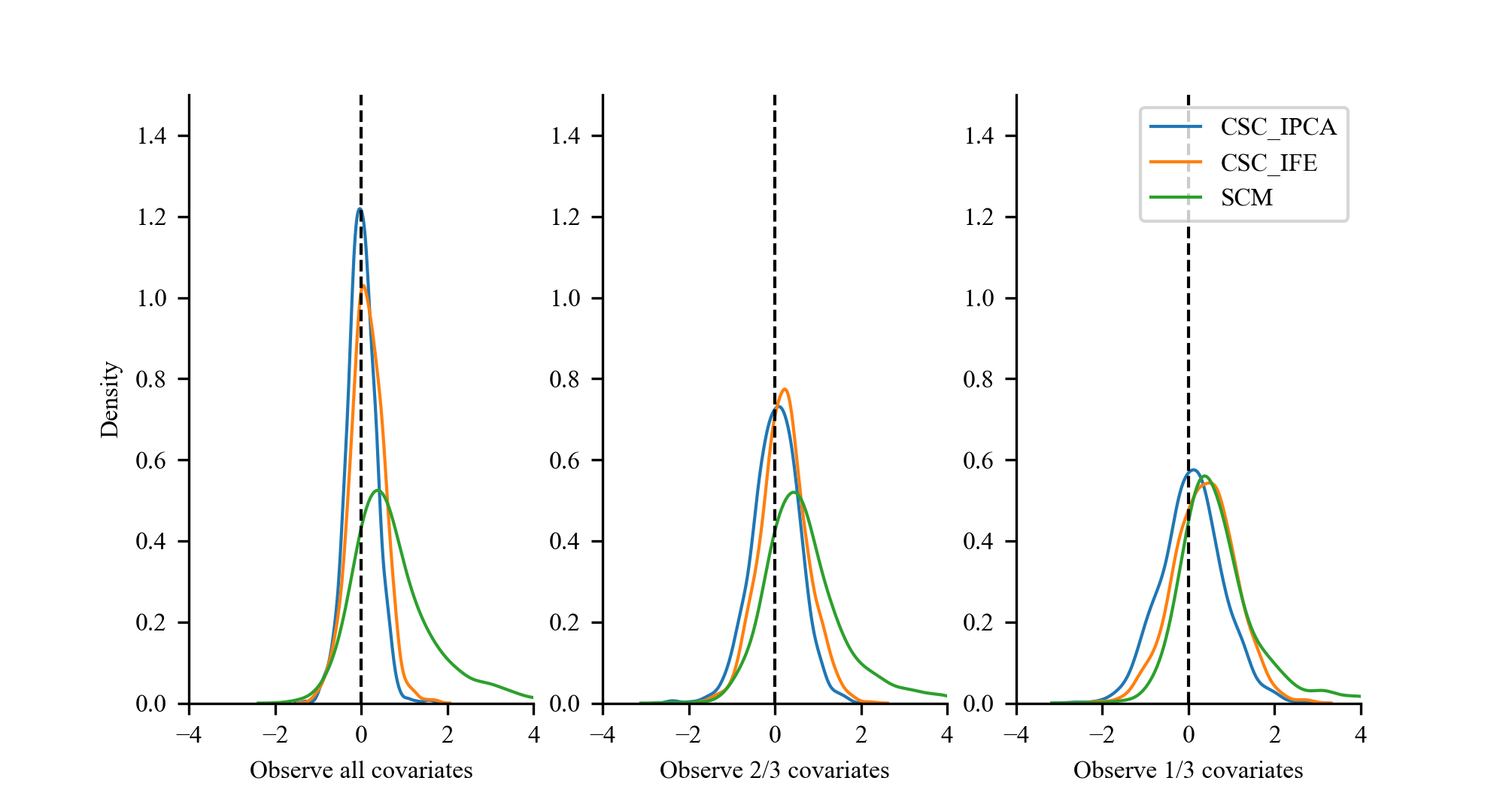
Figure C.4: Bias Comparison with Different DGPs

This figure plots the CSC-IPCA, CSC-IFE, and SCM method estimated ATT for simulated data with different data generating processes.

C.2 Finite sample properties

In this section, we provide additional simulation results to investigate the finite sample properties of the CSC-IFE and SCM methods for comparison.

Table C.2: Finite Sample Properties of CSC-IFE

$\alpha$		$1/3$	$2/3$	1	$1/3$	$2/3$	1	$1/3$	$2/3$	1
$T_{0}$	$N_{ctrl}$	Bias			RMSE			STD
10	10	6.478	3.184	0.045	7.996	4.311	0.747	4.701	2.939	0.854
10	20	6.173	2.885	-0.018	8.070	4.050	0.599	5.245	2.900	0.769
10	40	4.510	2.516	-0.007	6.785	3.931	0.527	5.096	3.044	0.675
20	10	6.650	3.536	-0.007	8.051	4.843	0.777	4.593	3.336	0.904
20	20	6.402	3.198	-0.013	8.085	4.529	0.587	4.939	3.272	0.740
20	40	5.690	2.555	0.001	7.633	3.864	0.570	5.111	2.935	0.720
40	10	7.353	3.523	-0.008	11.132	5.258	0.696	8.364	3.950	0.846
40	20	6.904	3.230	0.036	9.185	5.084	0.602	6.053	3.935	0.747
40	40	5.978	2.928	0.003	9.368	4.850	0.650	7.227	3.927	0.782

• This table presents the finite sample properties of the CSC-IFE method estimated ATT for simulated data. The number of treated units and post-treatment period is fixed to $N_{treat}=5,T_{1}=5$. We vary the number of control units $N_{ctrl}$, pre-treatment period $T_{0}$, and proportion of observed covariates $\alpha$ to investigate the finite sample properties, the total number of covariates is $L=9$. The bias, RMSE, and STD are estimated based on 1000 simulations.

Table C.3: Finite Sample Properties of SCM

$\alpha$		$1/3$	$2/3$	1	$1/3$	$2/3$	1	$1/3$	$2/3$	1
$T_{0}$	$N_{ctrl}$	Bias			RMSE			STD
10	10	10.026	10.188	9.909	10.997	11.323	10.964	4.554	4.960	4.721
10	20	9.874	10.007	9.924	11.011	11.168	11.028	4.872	4.991	4.840
10	40	9.720	10.088	9.521	10.891	11.388	10.655	4.936	5.304	4.808
20	10	10.596	10.526	10.674	12.036	11.841	12.149	5.714	5.454	5.816
20	20	10.269	10.250	10.113	11.935	11.671	11.745	6.109	5.614	5.985
20	40	9.719	9.654	10.206	11.309	11.206	12.353	5.810	5.699	6.986
40	10	10.678	11.069	11.117	12.794	12.946	13.705	7.087	6.731	8.033
40	20	10.970	11.207	11.148	13.719	13.459	13.601	8.249	7.451	7.780
40	40	10.742	10.851	10.221	13.303	13.786	12.684	7.853	8.520	7.539

• This table presents the finite sample properties of the SCM method estimated ATT for simulated data. The number of treated units and post-treatment period is fixed to $N_{treat}=5,T_{1}=5$. We vary the number of control units $N_{ctrl}$, pre-treatment period $T_{0}$, and proportion of observed covariates $\alpha$ to investigate the finite sample properties, the total number of covariates is $L=9$. The bias, RMSE, and STD are estimated based on 1000 simulations.

Appendix D Empirical Application

D.1 Data Description

In this section, we provide additional information on the data used in the empirical application. The main variable of interest is the FDI net inflow to GDP ratio. Based on this ratio, we exclude countries with values higher than 25% or lower than -25% to remove countries with extremely volatile FDI data. The excluded countries include Austria, Belgium, Hungary, Iceland, Ireland, Netherlands, Switerland and Luxembourg. As shown in Figure D.5, the FDI to GDP ratio is relatively stable in most countries, with the exception of the countries mentioned above. The final sample includes 30 OECD countries from 1995 to 2022.

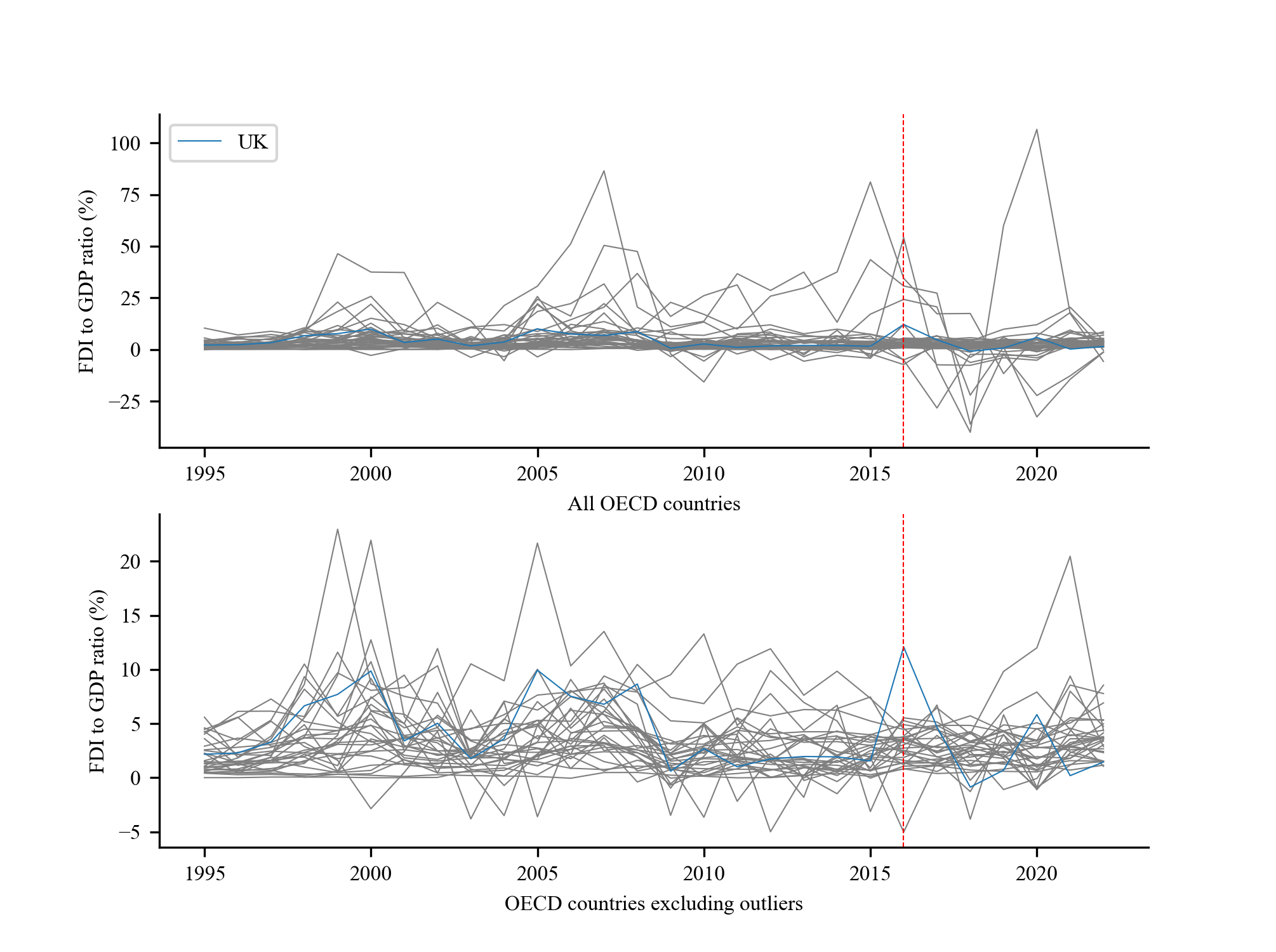
Figure D.5: FDI to GDP Ratio for Selected Countries

This figure plots the FDI to GDP ratio for selected OECD countries.

We provide the summary statistics of the data used in the empirical application in Table D.4. The variables include log GDP, log GDP per capita, import to GDP ratio, export to GDP ratio, GDP deflator, capital formation to GDP ratio, unemployment rate, employment to population ratio, log population, and FDI to GDP ratio.

Table D.4: Summary Statistics of the Data

	Count	Mean	Std	Min	25%	50%	75%	Max
Log GDP	840	26.65	1.64	23.05	25.77	26.46	27.89	30.69
Log GDP per Capita	840	10.01	0.71	8.28	9.46	10.14	10.60	11.28
Import to GDP	840	37.60	17.08	7.57	27.07	32.72	44.08	104.65
Export to GDP	840	37.60	17.78	8.82	25.78	34.20	44.72	99.30
GDP Deflator	840	87.53	34.04	1.29	73.15	89.95	100.41	707.41
Capital Formation to GDP	840	23.60	4.37	11.89	20.86	23.08	25.78	41.56
Unemployment Rate	840	8.23	4.24	2.02	5.11	7.41	10.28	27.69
Employment to Population	840	55.29	5.80	37.38	51.56	56.39	59.49	68.96
Log Population	840	16.64	1.40	14.09	15.49	16.35	17.88	19.62
FDI to GDP	840	3.11	2.90	-5.03	1.30	2.53	4.32	22.95

• This table presents the summary statistics of the data used in the empirical application.

We use different model specifications to investigate the relationship between the FDI to GDP ratio and other variables. The results are presented in Table D.5. The significance of the variables varies across the models, raising uncertainty about which variables are predictive and should be included in the final model. Fortunately, the CSC-IPCA method allows us to bypass the model selection process by incorporating all variables in the final model.

Table D.5: Regression Results

	Model 1	Model 2	Model 3	Model 4
Intercept	4.2650	4.2272	-30.9338	-51.1866
	(3.4547)	(3.3835)	(24.0543)	(35.8816)
Log GDP	-0.2595***	-0.2938***	0.4932	1.0023
	(0.0692)	(0.0674)	(0.5019)	(0.7904)
Log GDP per Capita	-0.2978**	-0.3432***	-0.4165	-0.2885
	(0.1171)	(0.1125)	(0.7746)	(0.7574)
Import to GDP	0.0076	-0.0088	-0.1233***	-0.0801*
	(0.0243)	(0.0238)	(0.0409)	(0.0418)
Export to GDP	0.0179	0.0304	0.1389***	0.0850**
	(0.0221)	(0.0214)	(0.0397)	(0.0387)
GDP Deflator	-0.0056*	-0.0067*	-0.0067*	-0.0039
	(0.0030)	(0.0036)	(0.0039)	(0.0039)
Capital Formation to GDP	0.0646**	0.0368	0.2544***	0.1152**
	(0.0250)	(0.0257)	(0.0456)	(0.0491)
Unemployment Rate	0.0935**	0.1196***	0.0870	0.0899
	(0.0370)	(0.0362)	(0.0594)	(0.0585)
Employment to Population	0.0967***	0.1054***	0.0425	0.0604
	(0.0259)	(0.0250)	(0.0639)	(0.0622)
Log Population	0.0383	0.0494	0.9097	1.2908
	(0.0838)	(0.0805)	(1.0455)	(1.1990)
Obs	840	840	840	840
R-squared	0.1242	0.2245	0.3485	0.4328
R-squared Adj.	0.1158	0.1907	0.3184	0.3860
Time FE	No	Yes	No	No
Country FE	No	No	Yes	No
TWFE	No	No	No	Yes
${}^{*}p<0.1,\ ^{**}p<0.05,\ ^{***}p<0.01$

• This table presents the regression results of the FDI to GDP ratio on other variables. The standard errors are reported in parentheses.

References

- Abadie and Imbens (2006) Alberto Abadie and Guido W Imbens. Large sample properties of matching estimators for average treatment effects. econometrica, 74(1):235–267, 2006.
- Abadie and Imbens (2011) Alberto Abadie and Guido W Imbens. Bias-corrected matching estimators for average treatment effects. Journal of Business & Economic Statistics, 29(1):1–11, 2011.
- Abadie et al. (2010) Alberto Abadie, Alexis Diamond, and Jens Hainmueller. Synthetic control methods for comparative case studies: Estimating the effect of california’s tobacco control program. Journal of the American statistical Association, 105(490):493–505, 2010.
- Arkhangelsky et al. (2021) Dmitry Arkhangelsky, Susan Athey, David A Hirshberg, Guido W Imbens, and Stefan Wager. Synthetic difference-in-differences. American Economic Review, 111(12):4088–4118, 2021.
- Arnorsson and Zoega (2018) Agust Arnorsson and Gylfi Zoega. On the causes of brexit. European Journal of Political Economy, 55:301–323, 2018.
- Ashenfelter (1978) Orley Ashenfelter. Estimating the effect of training programs on earnings. The Review of Economics and Statistics, pages 47–57, 1978.
- Athey et al. (2021) Susan Athey, Mohsen Bayati, Nikolay Doudchenko, Guido Imbens, and Khashayar Khosravi. Matrix completion methods for causal panel data models. Journal of the American Statistical Association, 116(536):1716–1730, 2021.
- Bai (2009) Jushan Bai. Panel data models with interactive fixed effects. Econometrica, 77(4):1229–1279, 2009.
- Bai and Ng (2002) Jushan Bai and Serena Ng. Determining the number of factors in approximate factor models. Econometrica, 70(1):191–221, 2002.
- Bai and Perron (2003) Jushan Bai and Pierre Perron. Computation and analysis of multiple structural change models. Journal of applied econometrics, 18(1):1–22, 2003.
- Ben-Michael et al. (2021) Eli Ben-Michael, Avi Feller, and Jesse Rothstein. The augmented synthetic control method. Journal of the American Statistical Association, 116(536):1789–1803, 2021.
- Brave (2009) Scott Brave. The chicago fed national activity index and business cycles. Chicago Fed Letter, (Nov), 2009.
- Card and Krueger (1993) David Card and Alan B Krueger. Minimum wages and employment: A case study of the fast food industry in new jersey and pennsylvania, 1993.
- Chan et al. (2016) Marc Chan, Simon Kwok, et al. Policy evaluation with interactive fixed effects. Preprint. Available at https://ideas. repec. org/p/syd/wpaper/2016-11. html, 2016.
- Chernozhukov et al. (2021) Victor Chernozhukov, Kaspar Wüthrich, and Yinchu Zhu. An exact and robust conformal inference method for counterfactual and synthetic controls. Journal of the American Statistical Association, 116(536):1849–1864, 2021.
- Colantone and Stanig (2018) Italo Colantone and Piero Stanig. Global competition and brexit. American political science review, 112(2):201–218, 2018.
- Connor and Korajczyk (1993) Gregory Connor and Robert A Korajczyk. A test for the number of factors in an approximate factor model. the Journal of Finance, 48(4):1263–1291, 1993.
- Dhingra et al. (2016) Swati Dhingra, Gianmarco Ottaviano, Thomas Sampson, and John Van Reenen. The impact of brexit on foreign investment in the uk. BREXIT 2016, 24(2):1–10, 2016.
- Eberhardt and Bond (2009) Markus Eberhardt and Stephen Bond. Cross-section dependence in nonstationary panel models: a novel estimator. 2009.
- Feng et al. (2020) Guanhao Feng, Stefano Giglio, and Dacheng Xiu. Taming the factor zoo: A test of new factors. The Journal of Finance, 75(3):1327–1370, 2020.
- Gobillon and Magnac (2016) Laurent Gobillon and Thierry Magnac. Regional policy evaluation: Interactive fixed effects and synthetic controls. Review of Economics and Statistics, 98(3):535–551, 2016.
- Higham (2009) Nicholas J Higham. Cholesky factorization. Wiley interdisciplinary reviews: computational statistics, 1(2):251–254, 2009.
- Hsiao et al. (2012) Cheng Hsiao, H Steve Ching, and Shui Ki Wan. A panel data approach for program evaluation: measuring the benefits of political and economic integration of hong kong with mainland china. Journal of Applied Econometrics, 27(5):705–740, 2012.
- Imbens (2024) Guido W Imbens. Causal inference in the social sciences. Annual Review of Statistics and Its Application, 11, 2024.
- Imbens and Rubin (2015) Guido W Imbens and Donald B Rubin. Causal inference in statistics, social, and biomedical sciences. Cambridge University Press, 2015.
- Jollife and Cadima (2016) Ian T Jollife and Jorge Cadima. Principal component analysis: A review and recent developments. Philos. Trans. R. Soc. A Math. Phys. Eng. Sci, 374(2065):20150202, 2016.
- Jolliffe (2002) Ian T Jolliffe. Principal component analysis for special types of data. Springer, 2002.
- Kelly et al. (2019) Bryan T Kelly, Seth Pruitt, and Yinan Su. Characteristics are covariances: A unified model of risk and return. Journal of Financial Economics, 134(3):501–524, 2019.
- Kelly et al. (2020) Bryan T Kelly, Seth Pruitt, and Yinan Su. Instrumented principal component analysis. Available at SSRN 2983919, 2020.
- Li (2018) Kathleen Li. Inference for factor model based average treatment effects. Available at SSRN 3112775, 2018.
- Neyman (1932) Jerzy Neyman. On the application of probability theory to agricultural experiments. essay on principles. section 9. Statistical Science, pages 465–472, 1932.
- Pesaran (2006) M Hashem Pesaran. Estimation and inference in large heterogeneous panels with a multifactor error structure. Econometrica, 74(4):967–1012, 2006.
- Rosenbaum and Rubin (1983) Paul R Rosenbaum and Donald B Rubin. The central role of the propensity score in observational studies for causal effects. Biometrika, 70(1):41–55, 1983.
- Roth et al. (2023) Jonathan Roth, Pedro HC Sant’Anna, Alyssa Bilinski, and John Poe. What’s trending in difference-in-differences? a synthesis of the recent econometrics literature. Journal of Econometrics, 235(2):2218–2244, 2023.
- Rubin (1974) Donald B Rubin. Estimating causal effects of treatments in randomized and nonrandomized studies. Journal of educational Psychology, 66(5):688, 1974.
- Rubin (1997) Donald B Rubin. Estimating causal effects from large data sets using propensity scores. Annals of internal medicine, 127(8_Part_2):757–763, 1997.
- Rubin (2005) Donald B Rubin. Causal inference using potential outcomes: Design, modeling, decisions. Journal of the American Statistical Association, 100(469):322–331, 2005.
- Shafer and Vovk (2008) Glenn Shafer and Vladimir Vovk. A tutorial on conformal prediction. Journal of Machine Learning Research, 9(3), 2008.
- Stock and Watson (2002) James H Stock and Mark W Watson. Forecasting using principal components from a large number of predictors. Journal of the American statistical association, 97(460):1167–1179, 2002.
- Welfens and Baier (2018) Paul JJ Welfens and Fabian J Baier. Brexit and foreign direct investment: Key issues and new empirical findings. International Journal of Financial Studies, 6(2):46, 2018.
- Xu (2017) Yiqing Xu. Generalized synthetic control method: Causal inference with interactive fixed effects models. Political Analysis, 25(1):57–76, 2017.