PREMAP: A Unifying PREiMage APproximation Framework for Neural Networks

Abstract

Most methods for neural network verification focus on bounding the image, i.e., set of outputs for a given input set. This can be used to, for example, check the robustness of neural network predictions to bounded perturbations of an input. However, verifying properties concerning the preimage, i.e., the set of inputs satisfying an output property, requires abstractions in the input space. We present a general framework for preimage abstraction that produces under- and over-approximations of any polyhedral output set. Our framework employs cheap parameterised linear relaxations of the neural network, together with an anytime refinement procedure that iteratively partitions the input region by splitting on input features and neurons. The effectiveness of our approach relies on carefully designed heuristics and optimization objectives to achieve rapid improvements in the approximation volume. We evaluate our method on a range of tasks, demonstrating significant improvement in efficiency and scalability to high-input-dimensional image classification tasks compared to state-of-the-art techniques. Further, we showcase the application to quantitative verification and robustness analysis, presenting a sound and complete algorithm for the former and providing sound quantitative results for the latter.

Keywords: preimage approximation, abstraction and refinement, linear relaxation, formal verification, neural network

1 Introduction

Despite the remarkable empirical success of neural networks, ensuring their safety against potentially adversarial behaviour, especially when using them as decision-making components in autonomous systems (Bojarski et al., 2016; Codevilla et al., 2018; Yun et al., 2017), is an important and challenging task. Towards this aim, various approaches have been developed for the verification of neural networks, with extensive effort devoted, in particular, to the problem of local robustness verification, which focuses on deciding the presence or absence of adversarial examples (Szegedy et al., 2013; Biggio et al., 2013) within an $\epsilon$-perturbation neighbourhood (Huang et al., 2017; Katz et al., 2017; Zhang et al., 2018; Bunel et al., 2018; Tjeng et al., 2019; Singh et al., 2019; Xu et al., 2020, 2021; Wang et al., 2021b).

While local robustness verification is useful for certifying that a neural network has the same prediction in a neighbourhood of an input, it does not provide finer-grained information on the behaviour of the network in the input domain. An alternative and more general approach for neural network analysis is to construct the preimage abstraction of its predictions (Matoba and Fleuret, 2020; Dathathri et al., 2019). Given a set of outputs, the preimage is defined as the set of all inputs mapped by the neural network to that output set. For example, given a particular action for a neural network controller (e.g., drive left), the preimage captures the set of percepts (e.g., car positions) that cause the neural network to take this action. By characterizing the preimage symbolically in an abstract representation, e.g., polyhedra, one can perform more complex analysis for a wider class of properties beyond local robustness, such as computing the proportion of inputs satisfying a property (Webb et al., 2019b; Mangal et al., 2019), or performing downstream reasoning tasks.

Unfortunately, exact preimage generation (Matoba and Fleuret, 2020) is intractable at scale, as it requires splitting into input subregions where the neural network is linear. Each such subregion corresponds to a set of determined activation patterns of the nonlinear neurons, the number of which grows exponentially with the number of neurons. Therefore, we focus on the problem of preimage approximation, that is, constructing symbolic abstractions for the preimage. In this work, we propose a general framework for preimage approximation that computes under-approximations and over-approximations represented as disjoint unions of polytopes (DUP).

Our method leverages recent progress in local robustness verification, which uses parameterized linear relaxations of neural networks together with branch-and-bound refinement strategies to analyze the input space in an efficient and GPU-friendly manner (Zhang et al., 2018; Wang et al., 2021b). We observe that, unlike robustness verification, where the goal is to determine the behaviour of the neural network at the worst-case point in the input space (and thus verify or falsify the property), in preimage approximation we instead aim to minimize the overall difference in volume between the approximation and the (intractable) exact preimage. Thus, we design a methodology that focuses on effectively optimising this new volume-based objective, while maintaining the GPU parallelism, efficiency, and flexibility drawn from the state-of-the-art robustness verifiers.

In more detail, this paper makes the following novel contributions:

1. the first unifying framework capable of efficiently generating symbolic under- and over-approximations of the preimage abstraction of any polyhedron output set;

2. an efficient and anytime preimage refinement algorithm, which iteratively partitions the input region into subregions using input and/or intermediate (ReLU) splitting (hyper)planes;

3. carefully-designed heuristics for selecting input features and neurons to split on, which (i) take advantage of GPU parallelism for efficient evaluation; and (ii) significantly improve approximation quality compared to naïve baselines;

4. a novel differentiable optimisation objective for improving preimage approximation precision, with respect to (i) convex bounding parameters of nonlinear neurons and (ii) Lagrange multipliers for neuron splitting constraints;

5. empirical evaluation of preimage approximation on a range of datasets, and an application to the problem of quantitative verification;

6. a publicly-available software implementation of our preimage approximation framework.

This work significantly extends the preliminary version in Zhang et al. (2024) in the following ways: (i) introducing an over-approximation algorithm within the framework, with accompanying empirical results; (ii) improving the refinement procedure through new heuristics for selecting input features to split on, using only 49.7% (avg.) computation time of the prior method to achieve the same precision (Sections 4.3, 5.2.2); (iii) introducing Lagrangian relaxation to enforce neuron splitting constraints, enabling further optimisation of the approximations with precision gains of up to 58.6% (avg.) for a MNIST preimage approximation task (Sections 4.5, 5.2.3); and (iv) an extended empirical evaluation of the framework.

The paper is organized as follows. Section 2 introduces the notation and preliminary definitions of neural networks, linear relaxation and polyhedra representations. In Section 3, we present the formulation of the problems studied, namely preimage approximation and quantitative analysis of neural networks. Our preimage approximation method is provided in Section 4, together with the application to quantitative verification of neural networks and proofs of soundness and completeness. In Section 5, we present the experimental evaluation of our approach and demonstrate its effectiveness and scalability compared to the state-of-the-art techniques, and applications in quantitative verification and robustness analysis. Finally, we discuss related works in Section 6 and conclude the paper in Section 7.

(a) Standard NN Verification: decide whether $f(x)\in O,\forall x\in\mathcal{C}$.

(b) NN Preimage Approximation: characterize $f^{-1}(O)\mathrel{\mathop{\mathchar 58\relax}}=\{x\in\mathcal{C}\mid f(x)\in O\}$.

Figure 1: Illustration of the preimage approximation problem. In contrast to NN robustness verification, where the goal is to answer Yes or No for the statement $f(x)\in O,\forall x\in\mathcal{C}$, in preimage approximation the goal is to find a bounding under-approximation and over-approximation to the preimage $f^{-1}(O)$. indicates the region where $f(x)\in O$.

2 Preliminaries

We use $f\mathrel{\mathop{\mathchar 58\relax}}\mathbb{R}^{d}\to\mathbb{R}^{m}$ to denote a feed-forward neural network. For layer $i$, we use $\textbf{W}^{(i)}$ to denote the weight matrix, $\textbf{b}^{(i)}$ the bias, $\textbf{z}^{(i)}$ the pre-activation neurons, and $\hat{\textbf{z}}^{(i)}$ the post-activation neurons, such that we have $\textbf{z}^{(i)}=\textbf{W}^{(i)}\hat{\textbf{z}}^{(i-1)}+\textbf{b}^{(i)}$. We use $h^{(i)}(x)$ to denote the function from input to pre-activation neurons, and $a^{(i)}(x)$ the function from input to the post-activation neurons, i.e., $\textbf{z}^{(i)}=h^{(i)}(x)$ and $\hat{\textbf{z}}^{(i)}=a^{(i)}(x)$. In this paper, we focus on ReLU neural networks with $a^{(i)}(x)=\textnormal{ReLU}(h^{(i)}(x))$, where $\textnormal{ReLU}(h)\mathrel{\mathop{\mathchar 58\relax}}=\max(h,0)$ is applied element-wise. However, our method can be generalized to other activation functions that can be bounded by linear functions, similarly to Zhang et al. (2018).

Linear Relaxation of Neural Networks. Nonlinear activation functions lead to the NP-completeness of the neural network verification problem as proved in Katz et al. (2017). To address such intractability, linear relaxation is often used to transform the nonconvex constraints into linear programs. As shown in Figure 2, given concrete lower and upper bounds $\textbf{l}^{(i)}\leq h^{(i)}(x)\leq\textbf{u}^{(i)}$ on the pre-activation values of layer $i$, there are three cases to consider. In the inactive ($u^{(i)}_{j}\leq 0$) and active ($l^{(i)}_{j}\geq 0)$ cases, the post-activation neurons $a^{(i)}_{j}(x)$ are linear functions $a^{(i)}_{j}(x)=0$ and $a^{(i)}_{j}(x)=h^{(i)}_{j}(x)$ respectively. In the unstable case, $a^{(i)}_{j}(x)$ can be bounded by $\alpha^{(i)}_{j}h^{(i)}_{j}(x)\leq a^{(i)}_{j}(x)\leq-\frac{u^{(i)}_{j}l^{(i)}_{j}}{u^{(i)}_{j}-l^{(i)}_{j}}+\frac{u^{(i)}_{j}}{u^{(i)}_{j}-l^{(i)}_{j}}h^{(i)}_{j}(x)$, where $\alpha^{(i)}_{j}$ is a configurable parameter that produces a valid lower bound for any value in $[0,1]$. Linear bounds can also be obtained for other non-piecewise linear activation functions by considering the characteristics of the activation function, such as the S-shape activation functions (Zhang et al., 2018; König et al., 2024).

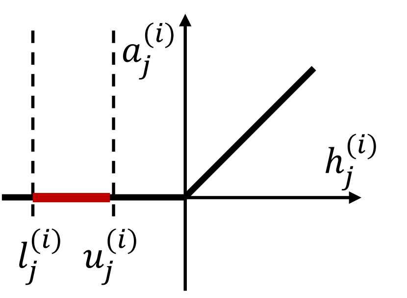
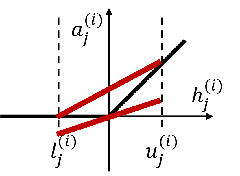
Figure 2: Linear bounding functions for inactive, active, unstable ReLU neurons.

Linear relaxation can be used to compute linear lower and upper bounds of the form $\underline{\textbf{A}}x+\underline{\textbf{b}}\leq f(x)\leq\overline{\textbf{A}}x+\overline{\textbf{b}}$ on the output of a neural network, for a given bounded input region $\mathcal{C}$. These methods are known as linear relaxation based perturbation analysis (LiRPA) algorithms (Xu et al., 2020, 2021; Singh et al., 2019). In particular, backward-mode LiRPA computes linear bounds on $f$ by propagating linear bounding functions backward from the output, layer by layer, to the input layer.

Polytope Representations. Given an Euclidean space $\mathbb{R}^{d}$, a polyhedron $T$ is defined to be the intersection of a set of half spaces. More formally, suppose we have a set of linear constraints defined by $\psi_{i}(x)\mathrel{\mathop{\mathchar 58\relax}}=c_{i}^{T}x+d_{i}\geq 0$ for $i=1,...K$, where $c_{i}\in\mathbb{R}^{d},d_{i}\in\mathbb{R}$ are constants, and $x=(x_{1},...,x_{d})$ is a tuple of variables. Then a polyhedron is defined as $T=\{x\in\mathbb{R}^{d}|\bigwedge_{i=1}^{K}\psi_{i}(x)\}$, where $T$ consists of all values of $x$ satisfying the first-order logic (FOL) formula $\alpha(x)\mathrel{\mathop{\mathchar 58\relax}}=\bigwedge_{i=1}^{K}\psi_{i}(x)$. We use the term polytope to refer to a bounded polyhedron, that is, a polyhedron $T$ such that $\exists R\in\mathbb{R}^{>0}\mathrel{\mathop{\mathchar 58\relax}}\forall x_{1},x_{2}\in T$, $\mathinner{\!\left\lVert x_{1}-x_{2}\right\rVert}_{2}\leq R$ holds. The abstract domain of polyhedra has been widely used for the verification of neural networks and computer programs as in Singh et al. (2019); Benoy (2002); Boutonnet and Halbwachs (2019). An important type of polytope is the hyperrectangle (box), which is a polytope defined by a closed and bounded interval $[\underline{x_{i}},\overline{x_{i}}]$ for each dimension, where $\underline{x_{i}},\overline{x_{i}}\in\mathbb{Q}$. More formally, using the linear constraints $\phi_{i}\mathrel{\mathop{\mathchar 58\relax}}=(x_{i}\geq\underline{x_{i}})\wedge(x_{i}\leq\overline{x_{i}})$ for each dimension, the hyperrectangle takes the form $\mathcal{C}=\{x\in\mathbb{R}^{d}|x\models\bigwedge_{i=1}^{d}\phi_{i}\}$.

3 Problem Formulation

3.1 Preimage Approximation

In this work, we are interested in the problem of computing preimages for neural networks. Given a subset $O\subset\mathbb{R}^{m}$ of the codomain, the preimage of a function $f\mathrel{\mathop{\mathchar 58\relax}}\mathbb{R}^{d}\to\mathbb{R}^{m}$ is defined to be the set of all inputs $x\in\mathbb{R}^{d}$ that are mapped to an element of $O$ by $f$. For neural networks in particular, the input is typically restricted to some bounded input region $\mathcal{C}\subset\mathbb{R}^{d}$. In this work, we restrict the output set $O$ to be a polyhedron, and the input set $\mathcal{C}$ to be an axis-aligned hyperrectangle region $\mathcal{C}\subset\mathbb{R}^{d}$, as these are commonly used in neural network verification. We now define the notion of a restricted preimage.

Definition 1 (Restricted Preimage)

Given a neural network $f\mathrel{\mathop{\mathchar 58\relax}}\mathbb{R}^{d}\to\mathbb{R}^{m}$, and an input set $\mathcal{C}\subset\mathbb{R}^{d}$, the restricted preimage of an output set $O\subset\mathbb{R}^{m}$ is defined to be the set $f^{-1}_{\mathcal{C}}(O)\mathrel{\mathop{\mathchar 58\relax}}=\{x\in\mathbb{R}^{d}|f(x)\in O\wedge x\in\mathcal{C}\}$.

Example 1

To illustrate our problem formulation and approach, we introduce a vehicle parking task from Ayala et al. (2011) as a running example. In this task, there are four parking lots, located in each quadrant of a $2\times 2$ grid $[0,2]^{2}$, and a neural network with two hidden layers of 10 ReLU neurons $f\mathrel{\mathop{\mathchar 58\relax}}\mathbb{R}^{2}\to\mathbb{R}^{4}$ is trained to classify which parking lot an input point belongs to. To analyze the behaviour of the neural network in the input region $[0,2]\times[0,2]$, we set $\mathcal{C}=\{x\in\mathbb{R}^{2}|(0\leq x_{1}\leq 2)\wedge(0\leq x_{2}\leq 2)\}$. Then the restricted preimage $f^{-1}_{\mathcal{C}}(O)$ of the set $O=\{y\in\mathbb{R}^{4}|\bigwedge_{i\in\{2,3,4\}}y_{1}-y_{i}\geq 0\}$ is the subspace of the region $[0,2]\times[0,2]$ that is labelled as parking lot $1$ by the neural network.

We focus on provable approximations of the preimage. Given a first-order formula $A$, $\alpha$ is an under-approximation (resp. over-approximation) of $A$ if it holds that $\forall x.\alpha(x)\implies A(x)$ (resp. $\forall x.A(x)\implies\alpha(x)$). In our context, the restricted preimage is defined by the formula $A(x)=(f(x)\in O)\wedge(x\in\mathcal{C})$, and we restrict to approximations $\alpha$ that take the form of a disjoint union of polytopes (DUP). The goal of our method is to generate a DUP approximation $\mathcal{T}$ that is as tight as possible; that is, we aim to maximize the volume $\textnormal{vol}(\mathcal{T})$ of an under-approximation, or minimize the volume $\textnormal{vol}(\mathcal{T})$ of an over-approximation.

Definition 2 (Disjoint Union of Polytopes)

A disjoint union of polytopes (DUP) is a FOL formula $\alpha$ of the form $\alpha(x)\mathrel{\mathop{\mathchar 58\relax}}=\bigvee_{i=1}^{D}\alpha_{i}(x)$, where each $\alpha_{i}$ is a polytope formula (conjunction of a finite set of linear half-space constraints), with the property that $\alpha_{i}\wedge\alpha_{j}$ is unsatisfiable for any $i\neq j$.

3.2 Quantitative Properties

One of the most important verification problems for neural networks is that of proving guarantees on the output of a network for a given input set (Gehr et al., 2018; Gopinath et al., 2020; Ruan et al., 2018). This is often expressed as a property of the form $(I,O)$ such that $\forall x\in I\implies f(x)\in O$. We can generalize this to quantitative properties:

Definition 3 (Quantitative Property)

Given a neural network $f\mathrel{\mathop{\mathchar 58\relax}}\mathbb{R}^{d}\to\mathbb{R}^{m}$, a measurable input set with non-zero measure (volume) $I\subseteq\mathbb{R}^{d}$, a measurable output set $O\subseteq\mathbb{R}^{m}$, and a rational proportion $p\in[0,1]$, we say that the neural network satisfies the property $(I,O,p)$ if $\frac{\textnormal{vol}(f^{-1}_{I}(O))}{\textnormal{vol}(I)}\geq p$.

Neural network verification algorithms can be characterized by two main properties: soundness, which states that the algorithm always returns correct results, and completeness, which states that the algorithm always reaches a conclusion on any verification query (Liu et al., 2021). We now define the soundness and completeness of verification algorithms for quantitative properties.

Definition 4 (Soundness)

A verification algorithm $QV$ is sound if, whenever $QV$ outputs True, the property $(I,O,p)$ holds.

Definition 5 (Completeness)

A verification algorithm $QV$ is complete if (i) $QV$ never returns Unknown, and (ii) whenever $QV$ outputs False, the property $(I,O,p)$ does not hold.

If the property $(I,O)$ holds, then the quantitative property $(I,O,1)$ holds, while quantitative properties for $0\leq p<1$ provide more information when $(I,O)$ does not hold. Most neural network verification methods produce approximations of the image of $I$ in the output space, which cannot be used to verify quantitative properties. Preimage over-approximations include points outside of the true preimage; thus, they cannot be applied for sound quantitative verification. In contrast, preimage under-approximations provide a lower bound on the volume of the preimage, allowing us to soundly verify quantitative properties.

4 Methodology

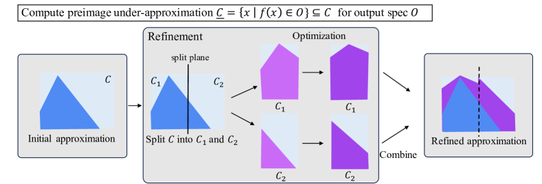
Figure 3: Illustration of the workflow for preimage under-approximation (shown in 2D for clarity). Given a neural network $f\mathrel{\mathop{\mathchar 58\relax}}\mathbb{R}^{d}\to\mathbb{R}^{m}$ and output specification $O\subset\mathbb{R}^{m}$, our algorithm generates an under-approximation $\underline{\mathcal{C}}$ to the preimage in the input region $\mathcal{C}$. Starting from the input region $\mathcal{C}$, the procedure repeatedly splits the selected region into smaller subregions $\mathcal{C}_{1}$ and $\mathcal{C}_{2}$ with tighter input bounds, and then optimises the bounding and Lagrangian parameters to increase the volume and thus improve the quality of the under-approximation. The refined under-approximation is combined into a union of polytopes.

4.1 Overview.

In this section, we present the main components of our methodology. Figure 3 shows the workflow of our preimage approximation method (using under-approximation as an illustration).

In Section 4.2, we introduce how to cheaply and soundly under-approximate (or over-approximate) the (restricted) preimage with a single polytope by means of the linear relaxation methods (Algorithm 2), which offer greater scalability than the exact method (Matoba and Fleuret, 2020). To handle the approximation loss caused by linear relaxation, in Section 4.3 we propose an anytime refinement algorithm that improves the approximation by partitioning a (sub)region into subregions with splitting (hyper)planes, with each subregion then being approximated more accurately in parallel. In Section 4.4, we propose a novel differentiable objective to optimise the bounding parameters of linear relaxation to tighten the polytope approximation. Next, in Section 4.5, we propose a refinement scheme based on intermediate ReLU splitting planes and derive a preimage optimisation method using Lagrangian relaxation of the splitting constraints. The main contribution of this paper (Algorithm 1) integrates these four components and is described in Section 4.6. Finally, in Section 4.7, we apply our method to quantitative verification (Algorithm 3) and prove its soundness and completeness.

To simplify the presentation, we focus on computing under-approximations and explain the necessary changes to compute over-approximations in highlight boxes throughout.

Input: Neural network $f$, Input region $\mathcal{C}$, Output region $O$, Volume threshold $v$, Maximum iterations $R$, Number of samples $N$, Boolean $Under$, Boolean $SplitOnInput$

Output: Disjoint union of polytopes $\mathcal{T}_{\textnormal{Dom}}$

$T$ $\leftarrow$ GenApprox($\mathcal{C}$, $O$, $N$, $Under$) ;

  // Initial preimage polytope

Dom $\leftarrow\{(\mathcal{C},T,\text{CalcPriority}(T,Under))\}$ ;

  // Priority queue

// $\mathcal{T}_{\textnormal{Dom}}$ is the union of the under/over-approximating polytopes in Dom

1 while $((\textnormal{Under}\textnormal{{ and }}\textnormal{EstimateVolume}(\mathcal{T}_{\textnormal{Dom}})<v)$ or $(\neg\textnormal{Under {and} }\textnormal{EstimateVolume}(\mathcal{T}_{\textnormal{Dom}})>v))$ and $\textnormal{Iterations}\leq R$  do

       $\mathcal{C}_{\text{sub}},T,\text{Priority}$ $\leftarrow$ Pop(Dom) ;

        // Subregion with highest priority

2       if SplitOnInput then

             $id$ $\leftarrow$ SelectInputFeature($\text{Feature}_{I},Under$) ;

              // $\text{Feature}_{I}$ is the set of input features/dimensions

3            

4      else

             $id\leftarrow$ SelectReLUNode($\text{Node}_{Z},Under$);

              // $\text{Node}_{Z}$ is the set of unstable ReLU nodes

5            

      [$\mathcal{C}_{sub}^{l}$,$\mathcal{C}_{sub}^{u}$] $\leftarrow$ SplitOnNode($\mathcal{C}_{sub}$, $id$);

        // Split on the selected node

       $T^{l},T^{u}$$\leftarrow$ GenApprox([$\mathcal{C}_{sub}^{l}$,$\mathcal{C}_{sub}^{u}$], $O$, $N,Under$) ;

        // Generate preimage

       Dom $\leftarrow$ Dom $\cup$ {($\mathcal{C}_{sub}^{l},T^{l}$,$\text{CalcPriority}(T^{l},Under)$), ($\mathcal{C}_{sub}^{u},T^{r}$,$\text{CalcPriority}(T^{r},Under)$)};

        // Disjoint polytope

6      

return $\mathcal{T}_{\textnormal{Dom}}$

Algorithm 1 Preimage Approximation

4.2 Polytope Approximation via Linear Relaxation

We first show how to adapt linear relaxation techniques to efficiently generate valid under-approximations and over-approximations to the restricted preimage for a given input region $\mathcal{C}$ as a single polytope. Recall that LiRPA methods enable us to obtain linear lower and upper bounds on the output of a neural network $f$, that is, $\underline{\textbf{A}}x+\underline{\textbf{b}}\leq f(x)\leq\overline{\textbf{A}}x+\overline{\textbf{b}}$, where the linear coefficients depend on the input region $\mathcal{C}$.

Suppose that we are given the input hyperrectangle $\mathcal{C}=\{x\in\mathbb{R}^{d}|x\models\bigwedge_{i=1}^{d}\phi_{i}\}$, and the output polytope specified using the half-space constraints $\psi_{i}(y)=(c_{i}^{T}y+d_{i}\geq 0)$ for $i=1,...,K$ over the output space. Let us first consider generating a guaranteed under-approximation. Given a constraint $\psi_{i}$, we append an additional linear layer at the end of the network $f$, which maps $y\mapsto c_{i}^{T}y+d_{i}$, such that the function $g_{i}\mathrel{\mathop{\mathchar 58\relax}}\mathbb{R}^{d}\to\mathbb{R}$ represented by the new network is $g_{i}(x)=c_{i}^{T}f(x)+d_{i}$. Then, applying LiRPA lower bounding to each $g_{i}$, we obtain a lower bound $\underline{g_{i}}(x)=\underline{a}_{i}^{T}x+\underline{b}_{i}$ for each $i$, such that $\underline{g_{i}}(x)\geq 0\implies g_{i}(x)\geq 0$ for $x\in\mathcal{C}$. Notice that, for each $i=1,...,K$, $\underline{a}_{i}^{T}x+\underline{b}_{i}\geq 0$ is a half-space constraint in the input space. We conjoin these constraints, along with the restriction to the input region $\mathcal{C}$, to obtain a polytope:

$$\underline{T_{\mathcal{C}}}(O)\mathrel{\mathop{\mathchar 58\relax}}=\{x|\bigwedge_{i=1}^{K}(\underline{g_{i}}(x)\geq 0)\wedge\bigwedge_{i=1}^{d}\phi_{i}(x)\}$$ (1)

Proposition 6

$\underline{T_{\mathcal{C}}}(O),\overline{T_{\mathcal{C}}}(O)$ are respectively under- and over-approximations to the restricted preimage $f^{-1}_{\mathcal{C}}(O)$.

Proof  For the under-approximation, the LiRPA bound $\underline{g_{i}}(x)\leq g_{i}(x)$ holds for any $x\in\mathcal{C}$ and $i=1,...,K$, and so we have $\bigwedge_{i=1}^{K}(\underline{g_{i}}(x)\geq 0)\wedge x\in\mathcal{C}\implies\bigwedge_{i=1}^{K}(g_{i}(x)\geq 0)\wedge x\in\mathcal{C}$, i.e., $\underline{T_{\mathcal{C}}}(O)$ is an under-approximation to $f^{-1}_{\mathcal{C}}(O)$. Similarly, for the over-approximation, $g_{i}(x)\leq\overline{g_{i}}(x)$ holds for any $x\in\mathcal{C}$ and $i=1,...,K$, and so $\bigwedge_{i=1}^{K}(g_{i}(x)\geq 0)\wedge x\in\mathcal{C}\implies\bigwedge_{i=1}^{K}(\overline{g_{i}}(x)\geq 0)\wedge x\in\mathcal{C}$, i.e. $\overline{T_{\mathcal{C}}}(O)$ is an over-approximation to $f^{-1}_{\mathcal{C}}(O)$.

 

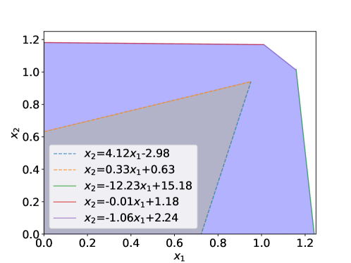
Figure 4: Illustration of initial preimage under- and over-approximation for output specification $\wedge_{i\in\{2,3,4\}}(y_{1}-y_{i}\geq 0)$ in the vehicle parking task (for more details see Example 2). The under-approximation is the polytope in grey, bounded by dotted half-planes, and the over-approximation is the polytope in blue, bounded by solid half-planes.

Example 2

Returning to Example 1, the output constraints (for $i=2,3,4$) are given by $\psi_{i}=(y_{1}-y_{i}\geq 0)=(c_{i}^{T}y+d_{i}\geq 0)$, where $c_{i}\mathrel{\mathop{\mathchar 58\relax}}=e_{1}-e_{i}$ (we use $e_{i}$ to denote the $i^{\text{th}}$ standard basis vector) and $d_{i}\mathrel{\mathop{\mathchar 58\relax}}=0$. Applying LiRPA bounding, we obtain the linear lower bounds $\underline{g_{2}}(x)=-4.12x_{1}+x_{2}+2.98\geq 0;\underline{g_{3}}(x)=0.33x_{1}-x_{2}+0.63\geq 0$; and $\underline{g_{4}}(x)$ (not shown). The intersection of these constraints, shown in Figure 4 (region in grey), represents an under-approximation to the preimage. Similarly, we can obtain linear upper bounds $\overline{g_{2}}(x)=-12.23x_{1}-x_{2}+15.18\geq 0;\overline{g_{3}}(x)=-0.01x_{1}-x_{2}+1.18\geq 0$; and $\overline{g_{4}}(x)=-1.06x_{1}-x_{2}+2.24\geq 0$; the intersection of those constraints represents an over-approximation to the preimage, as shown in Figure 4 (region in blue).

We generate the linear bounds in parallel over the output polyhedron constraints $i=1,...,K$ using the backward mode LiRPA (Zhang et al., 2018), and store the resulting approximating polytope as a list of constraints. This highly efficient procedure is used as a sub-routine LinearBounds when generating either preimage under-approximations or over-approximations in Algorithm 2 (Lines 2, 2).

Input: List of subregions $\mathcal{C}$, Output set $O$, Number of samples $N$, Boolean $Under$

Output: List of polytopes T

1

2$\textbf{T}=[]$;

for subregion $\mathcal{C}_{sub}\in\mathcal{C}$ // Parallel over subregions

3 do

4       $x_{1},...,x_{N}\leftarrow$ Sample($\mathcal{C}_{sub},N$);

5       if Under then

6             $[\underline{g_{1}}(x,\bm{\alpha}_{1},\bm{\beta}_{1}),...,\underline{g_{K}}(x,\bm{\alpha}_{K},\bm{\beta}_{K})]\leftarrow$ LinearLowerBound($\mathcal{C}_{sub},O$) ;

7            

8            Loss$(\bm{\alpha}_{1},...,\bm{\alpha}_{K},\bm{\beta}_{1},...,\bm{\beta}_{K})\leftarrow-\frac{\text{vol}(\mathcal{C}_{sub})}{N}\sum_{j=1,...,N}\sigma(-\textnormal{LSE}(-\underline{g_{1}}(x_{j},\bm{\alpha}_{1},\bm{\beta}_{1}),...,-\underline{g_{K}}(x_{j},\bm{\alpha}_{K},\bm{\beta}_{K})))$;

9             $\bm{\alpha}_{1}^{*},...,\bm{\alpha}_{K}^{*},\bm{\beta}_{1}^{*},...,\bm{\beta}_{K}^{*}\leftarrow\textnormal{argmin}(\textnormal{Loss}(\bm{\alpha}_{1},...,\bm{\alpha}_{K},\bm{\beta}_{1},...,\bm{\beta}_{K}))$;

10             $\textbf{T}=\textnormal{Append}(\textbf{T},[\underline{g_{1}}(x,\bm{\alpha}_{1}^{*},\bm{\beta}_{1}^{*})\geq 0,...,\underline{g_{K}}(x,\bm{\alpha}_{K}^{*},\bm{\beta}_{K}^{*})\geq 0,x\in\mathcal{C}_{sub}])$

11      else

12             $[\overline{g_{1}}(x,\bm{\alpha}_{1},\bm{\beta}_{1}),...,\overline{g_{K}}(x,\bm{\alpha}_{K},\bm{\beta}_{K})]\leftarrow$ LinearUpperBound($\mathcal{C}_{sub},O$) ;

13            

14            Loss$(\bm{\alpha}_{1},...,\bm{\alpha}_{K},\bm{\beta}_{1},...,\bm{\beta}_{K})\leftarrow\frac{\text{vol}(\mathcal{C}_{sub})}{N}\sum_{j=1,...,N}\sigma(-\textnormal{LSE}(-\overline{g_{1}}(x_{j},\bm{\alpha}_{1},\bm{\beta}_{1}),...,-\overline{g_{K}}(x_{j},\bm{\alpha}_{K},\bm{\beta}_{K})))$;

15             $\bm{\alpha}_{1}^{*},...,\bm{\alpha}_{K}^{*},\bm{\beta}_{1}^{*},...,\bm{\beta}_{K}^{*}\leftarrow\textnormal{argmin}(\textnormal{Loss}(\bm{\alpha}_{1},...,\bm{\alpha}_{K},\bm{\beta}_{1},...,\bm{\beta}_{K}))$;

16             $\textbf{T}=\textnormal{Append}(\textbf{T},[\overline{g_{1}}(x,\bm{\alpha}_{1}^{*},\bm{\beta}_{1}^{*})\geq 0,...,\overline{g_{K}}(x,\bm{\alpha}_{K}^{*},\bm{\beta}_{K}^{*})\geq 0,x\in\mathcal{C}_{sub}])$

17      

18

return T

Algorithm 2 GenApprox

4.3 Global Branching and Refinement

As LiRPA performs crude linear relaxation, the resulting bounds can be quite loose, even with optimisation over bounding parameters (as we will see in Section 4.4), meaning that the (single) polytope under-approximation or over-approximation is unlikely to be a good approximation to the preimage by itself. To address this challenge, we employ a divide-and-conquer approach that iteratively refines our approximation of the preimage. Starting from the initial region $\mathcal{C}$ at the root, our method generates a tree by iteratively partitioning a subregion $\mathcal{C}_{sub}$ represented at a leaf node into two smaller subregions $\mathcal{C}_{sub}^{l},\mathcal{C}_{sub}^{u}$, which are then attached as children to that leaf node. In this way, the subregions represented by all leaves of the tree are disjoint, such that their union is the initial region $\mathcal{C}$.

In order to under-approximate (resp. over-approximate) the preimage, for each leaf subregion $\mathcal{C}_{sub}$ we compute, using LiRPA bounds, an associated polytope that under-approximates (resp. over-approximates) the preimage in $\mathcal{C}_{sub}$. Thus, irrespective of the number of refinements performed, the union of the under-approximating polytopes (resp. over-approximating) corresponding to all leaves forms an anytime DUP under-approximation (resp. over-approximation) $\mathcal{T}$ to the preimage in the original region $\mathcal{C}$. The process of refining the subregions continues until an appropriate termination criterion is met.

Unfortunately, even with a moderate number of input dimensions or unstable ReLU nodes, naïvely splitting along all input- or ReLU-planes quickly becomes computationally intractable. For example, splitting a $d$-dimensional hyperrectangle using bisections along each dimension results in $2^{d}$ subdomains to approximate. It thus becomes crucial to prioritise the subregions to split, as well as improve the efficiency of the splitting procedure itself. We describe these in turn.

Subregion Selection.

We propose a subregion selection strategy that prioritises splitting subregions with the largest difference in volume between the exact preimage $f^{-1}_{\mathcal{C}_{sub}}(O)$ and the (already computed) polytope approximation $T_{\mathcal{C}_{sub}}(O)$ on that subdomain: this indicates “how much improvement” can be achieved on this subdomain and is implemented as the CalcPriority function in Algorithm 1. Unfortunately, computing the volume of a polytope exactly is a computationally expensive task, requiring specialised tools (Chevallier et al., 2022). To overcome this, we employ Monte Carlo estimation of volume computation by sampling $N$ points $x_{1},...,x_{N}$ uniformly from the input subdomain $\mathcal{C}_{sub}$. For an under-approximation, we have:

$$\textnormal{Priority}(\mathcal{C}_{sub}) \mathrel{\mathop{\mathchar 58\relax}}=\frac{\text{vol}(\mathcal{C}_{sub})}{N}\times\left(\sum_{i=1}^{N}\mathds{1}_{x_{i}\in f^{-1}_{\mathcal{C}_{sub}}(O)}-\sum_{i=1}^{N}\mathds{1}_{x_{i}\in\underline{T_{\mathcal{C}_{sub}}}(O)}\right)$$ (3)

$$\approx\textnormal{vol}(f^{-1}_{\mathcal{C}_{sub}}(O))-\textnormal{vol}(\underline{T_{\mathcal{C}_{sub}}}(O))$$ (4)

This measures the gap between the polytope under-approximation and the optimal approximation, namely, the preimage itself.

We then choose the leaf subdomain with the maximum priority. This leaf subdomain is then partitioned into two subregions $\mathcal{C}_{sub}^{l},\mathcal{C}_{sub}^{u}$, each of which we then approximate with polytopes $T_{\mathcal{C}_{sub}^{l}}(O),T_{\mathcal{C}_{sub}^{u}}(O)$. As tighter intermediate concrete bounds, and thus linear bounding functions, can be computed on the partitioned subregions, the polytope approximation on each subregion will be refined compared with the polytope approximation on the original subregion.

In the rest of this subsection, we consider how to split a leaf subregion into two subregions to optimise the volume of the preimage approximation. In particular, we propose two approaches: input splitting and ReLU splitting.

Input Splitting.

Given a subregion (hyperrectangle) defined by lower and upper bounds $x_{i}\in[\underline{x}_{i},\overline{x}_{i}]$ for all dimensions $i=1,...,d$, input splitting partitions it into two subregions by cutting along some feature $i$. This splitting procedure will produce two subregions that are similar to the original subregion, but have updated bounds $[\underline{x}_{i},\frac{\underline{x}_{i}+\overline{x}_{i}}{2}],[\frac{\underline{x}_{i}+\overline{x}_{i}}{2},\overline{x}_{i}]$ for feature $i$ instead. A commonly-adopted splitting heuristic is to select the dimension with the longest edge (Bunel et al., 2020), that is, to select feature $i$ with the largest range: $\arg\max_{i}(\overline{x}_{i}-\underline{x}_{i})$. However, this method does not perform well in terms of per-iteration volume improvement of the preimage approximation.

Thus, we propose to greedily select a dimension instead according to a volume-aware heuristic. Specifically, for each feature, we generate approximating polytopes $T^{l},T^{r}$ for the two subregions resulting from the split, and choose the feature that maximises the following priority metric. In the case of under-approximation, when $T^{l}$ consists of linear lower bounds $\underline{g_{1}}^{l},\ldots,\underline{g_{K}}^{l}$ and $T^{r}$ consists of linear lower bounds $\underline{g_{1}}^{r},\ldots,\underline{g_{K}}^{r}$, we define:

$$\text{InputPriority}(T^{l},T^{r})\mathrel{\mathop{\mathchar 58\relax}}=\frac{\text{vol}(\mathcal{C}_{sub})}{N}\left(\sum_{j=1}^{N}\sigma\left(\min_{i=1,...K}\underline{g_{i}^{l}}(x_{j})\right)+\sum_{j=1}^{N}\sigma\left(\min_{i=1,...K}\underline{g_{i}^{r}}(x_{j})\right)\right)$$ (7)

where $\sigma$ is the sigmoid function $\sigma(y)\mathrel{\mathop{\mathchar 58\relax}}=\frac{1}{1+e^{-y}}$. Intuitively, this is an approximation to the (total) volume of the under-approximating polytopes (e.g., $x_{j}$ is in the polytope $T_{l}$ iff $\min_{i=1,...K}\underline{g_{i}^{l}}(x_{j})>0$); we should prefer to split on input features that maximise the total volume. However, we found empirically that, in early iterations of the refinement, the under-approximation could often be empty (as the set $\{\min_{i=1,...,K}\underline{g_{i}^{l}}(x_{j})>0\}$ for all $i$ lies outside the subregion $\mathcal{C}_{sub}$), leading to zero priority for all features. For this reason, we propose to instead use the smooth sigmoid function to measure “how close” the constraints are to being satisfied for the sampled points, in order to provide signal for the best feature to split on.

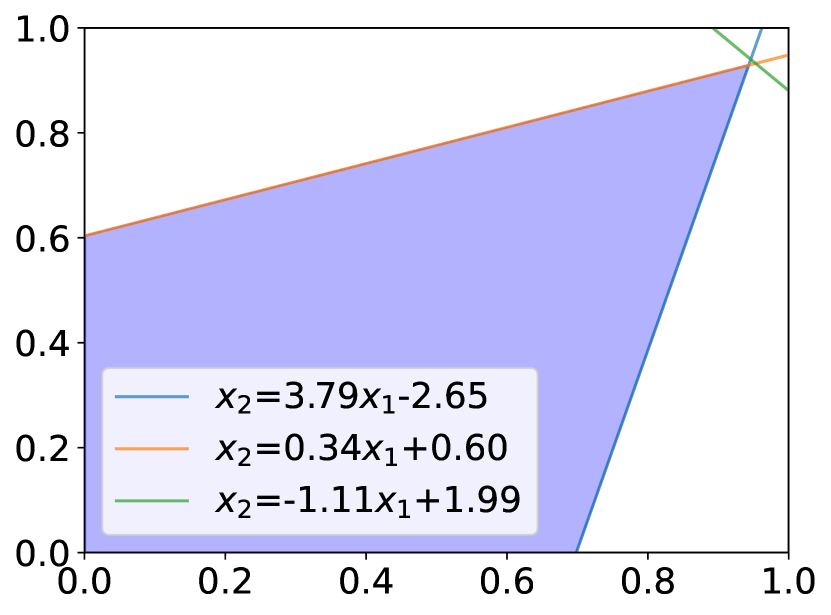
(a) Initial under-approximation

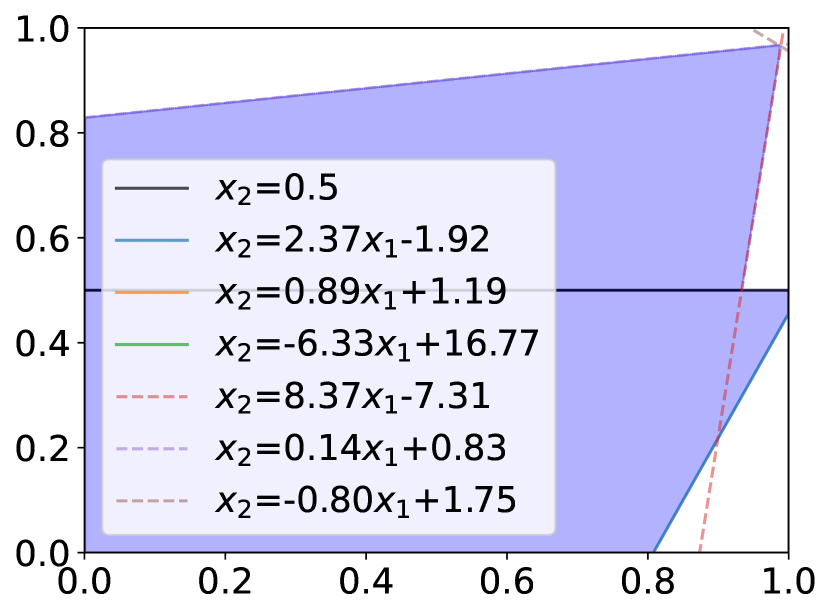
(b) Input split

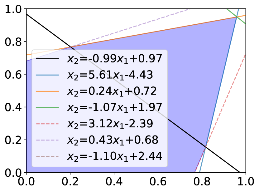
(c) ReLU split

Figure 5: Refinement of the initial preimage under-approximation with input and ReLU splitting. Figure 5(b) and 5(c) display the refined preimage, i.e., larger volume, after adding input and ReLU splitting planes, where the dotted and solid bounding planes are used to form the polytope on each subregion, respectively.

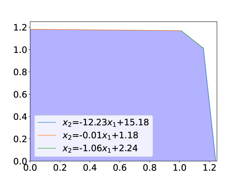
(a) Initial over-approximation

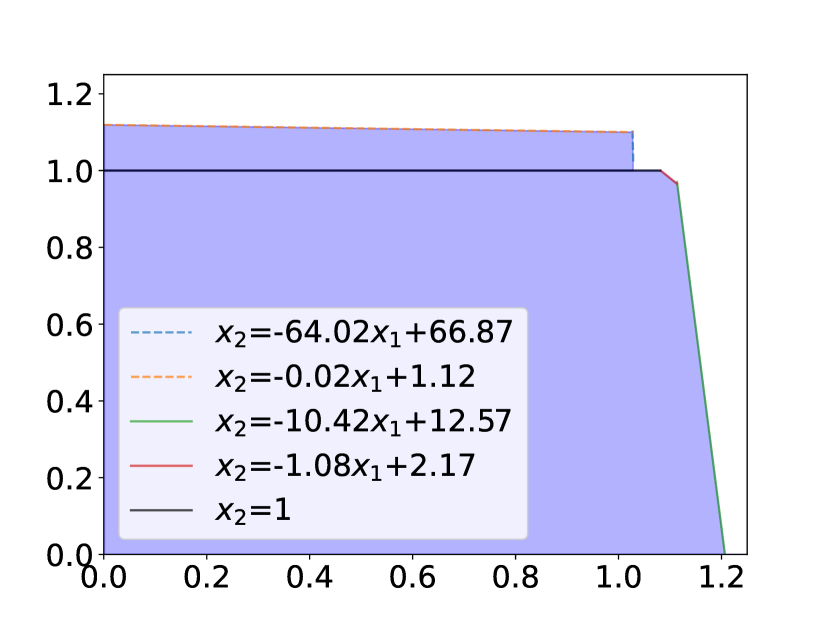
(b) Input split

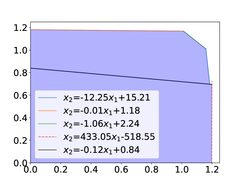
(c) ReLU split

Figure 6: Refinement of the initial preimage over-approximation with input and ReLU splitting. Figure 6(b) and 6(c) display the refined preimage, i.e., smaller volume, after adding input and ReLU splitting planes, where the dotted and solid bounding planes are used to form the polytope on each subregion, respectively.

Example 3

We revisit Example 1. Figure 5(a) shows the initial polytope under-approximation computed on the input region $\mathcal{C}$ before refinement, where each solid line represents the bounding plane for each output specification ($y_{1}-y_{i}\geq 0$). Figure 5(b) depicts the refined approximation by splitting the input region along the vertical axis, where the solid and dashed lines represent the bounding planes for the two resulting subregions. It can be seen that the total volume of the under-approximation has improved significantly. Similarly, in Figure 6(a), we show the initial polytope over-approximation before refinement, and in Figure 6(b) the improved over-approximation after greedy input splitting.

Intermediate ReLU Splitting. Refinement through splitting on input features is adequate for low-dimensional input problems such as reinforcement learning agents. However, it may be infeasible to generate sufficiently fine subregions for high-dimensional domains. We thus propose an algorithm for ReLU neural networks that uses intermediate ReLU splitting for preimage refinement. After determining a subregion for refinement, we partition the subregion based upon the pre-activation value of an intermediate unstable neuron $z^{(i)}_{j}=0$. As a result, the original subregion $\mathcal{C}_{sub}$ is split into two new subregions $\mathcal{C}^{+}_{z^{(i)}_{j}}=\{x\in\mathcal{C}_{sub}\leavevmode\nobreak\ |\leavevmode\nobreak\ z^{(i)}_{j}=h^{(i)}_{j}(x)\geq 0\}$ and $\mathcal{C}^{-}_{z^{(i)}_{j}}=\{x\in\mathcal{C}_{sub}\leavevmode\nobreak\ |\leavevmode\nobreak\ z^{(i)}_{j}=h^{(i)}_{j}(x)<0\}$.

In this procedure, the order of splitting unstable ReLU neurons can greatly influence the quality and efficiency of the refinement. Existing heuristic methods of ReLU prioritisation select ReLU nodes that lead to greater improvement in the final bound (maximum or minimum value) of the neural network on the input domain (Bunel et al., 2020), e.g., $\min_{x\in\mathcal{C}}\underline{f}(x)$. However, these ReLU prioritisation methods are not effective for preimage analysis, because our objective is instead to refine the overall preimage approximation. Thus, we compute (an estimate of) the volume difference between the split subregions $\lvert\textnormal{vol}(\mathcal{C}^{+}_{z^{(i)}_{j}})-\textnormal{vol}(\mathcal{C}^{-}_{z^{(i)}_{j}})\rvert$, using a single forward pass for a set of sampled data points from the input domain; note that this is bounded above by the total subregion volume $\textnormal{vol}(\mathcal{C}_{sub})$. We then propose to select the ReLU node that minimises this difference. Intuitively, this choice results in balanced subdomains after splitting.

A key advantage of ReLU splitting is that we can replace the unstable neuron bound $\underline{c}h^{(i)}_{j}(x)+\underline{d}\leq a^{(i)}_{j}(x)\leq\overline{c}h^{(i)}_{j}(x)+\overline{d}$ with the exact linear function $a^{(i)}_{j}(x)=h^{(i)}_{j}(x)$ and $a^{(i)}_{j}(x)=0$, respectively, as shown in Figure 2 (unstable to stable). This can typically tighten the approximation on each subdomain as the linear relaxation errors for this unstable neuron are removed for each subdomain and substituted with the exact symbolic function for backward propagation.

Example 4

We now apply our algorithm with ReLU splitting to the problem in Example 1. Figure 5(c) shows the refined preimage polytope by adding the splitting plane (black solid line) along the direction of a selected unstable ReLU node. Compared with Figure 5(a), we can see that the volume of the approximation increased. Similarly, in Figure 6(c), we show the improved over-approximation after ReLU splitting, compared to the initial over-approximation 6(a).

Combining Preimage Polytopes. As the final step, we combine the refined symbolic approximations on each subregion to compute the disjoint polytope union for the desired preimage of the output property. Note that the input splitting (hyper)planes naturally yield disjoint subregions. We can directly compute the final disjoint polytope union by combining the preimage polytopes of each subregion, where the splitting planes serve as part of the constraints that form the preimage polytope, e.g., two disjoint polytopes with the splitting constraints $x_{2}-0.5\geq 0$ and $-x_{2}+0.5\geq 0$, respectively, partitioned by $x_{2}=0.5$ in Figure 5(b). In the case of ReLU splitting, as each ReLU neuron represents a complex non-linear function with respect to the input, we cannot directly add the constraints introduced by ReLU splitting to the polytope representation. Instead, we compute the linear upper or lower bounding functions of the non-linear constraint represented by the ReLU neuron, i.e., $\underline{h^{(i)}_{j}}(x)\leq h^{(i)}_{j}(x)\leq\overline{h^{(i)}_{j}}(x)$. The constraints introduced by the linear bounding functions, i.e., $\underline{h^{(i)}_{j}}(x)\geq 0$ and $-\underline{h^{(i)}_{j}}(x)\geq 0$, can then be added to form disjoint polytopes. For instance, as shown in Figure 5(c), two disjoint polytopes are formed with the additional splitting constraints $-0.99x_{1}-x_{2}+0.97\geq 0$ and $0.99x_{1}+x_{2}-0.97\geq 0$, respectively, partitioned by the linear splitting plane $x_{2}=-0.99x_{1}+0.97$ (exact linear function of the selected ReLU neuron in this case). In fact, any linear function between the linear upper and lower bounding functions of the ReLU neuron serves as a valid splitting (hyper)plane to form disjoint polytopes.

4.4 Local Optimization

One of the key components behind the effectiveness of LiRPA-based bounds is the ability to efficiently improve the tightness of the bounding function by optimising the relaxation parameters $\bm{\alpha}$ via projected gradient descent. In the context of local robustness verification, the goal is to optimise the concrete (scalar) lower or upper bounds over the (sub)region $\mathcal{C}_{sub}$ (Xu et al., 2020), i.e., $\min_{x\in\mathcal{C}_{sub}}\underline{\textbf{A}}(\bm{\alpha})x+\underline{\textbf{b}}(\bm{\alpha})$ in the case of lower bounds, where we explicitly note the dependence of the linear coefficients on $\bm{\alpha}$. In our case, we are instead interested in optimising $\bm{\alpha}$ to refine the polytope approximation, that is, increase the volume of under-approximations and decrease the volume of over-approximations (to the exact preimage).

As before, we employ statistical estimation; we sample $N$ points $x_{1},...,x_{N}$ uniformly from the input domain $\mathcal{C}_{sub}$ then employ Monte Carlo estimation for the volume of the approximating polytope. In the case of under-approximation, we have:

$$\widehat{\textnormal{vol}}(\underline{T_{\mathcal{C}_{sub},\bm{\alpha}}}(O))=\frac{\text{vol}(\mathcal{C}_{sub})}{N}\times\sum_{i=1}^{N}\mathds{1}_{x_{i}\in\underline{T_{\mathcal{C}_{sub},\bm{\alpha}}}(O)}$$ (9)

where we highlight the dependence of $\underline{T_{\mathcal{C}_{sub}}}(O)=\{x|\bigwedge_{i=1}^{K}\underline{g_{i}}(x,\bm{\alpha}_{i})\geq 0\wedge\bigwedge_{i=1}^{d}\phi_{i}(x)\}$ on $\bm{\alpha}=(\bm{\alpha}_{1},...,\bm{\alpha}_{K})$, and $\bm{\alpha}_{i}$ are the $\alpha$-parameters for the linear relaxation of the neural network $g_{i}$ corresponding to the $i^{\textnormal{th}}$ half-space constraint in $O$. However, this is still non-differentiable w.r.t. $\bm{\alpha}$ due to the identity function. We now show how to derive a differentiable relaxation, which is amenable to gradient-based optimization:

$$\widehat{\textnormal{vol}}(\underline{T_{\mathcal{C}_{sub},\bm{\alpha}}}(O)) =\frac{\text{vol}(\mathcal{C}_{sub})}{N}\sum_{j=1}^{N}\mathds{1}_{x_{j}\in\underline{T_{\mathcal{C}_{sub},\bm{\alpha}}}(O)}=\frac{\text{vol}(\mathcal{C}_{sub})}{N}\sum_{j=1}^{N}\mathds{1}_{\min_{i=1,...K}\underline{g_{i}}(x_{j},\bm{\alpha}_{i})\geq 0}$$ (10)

$$\approx\frac{\text{vol}(\mathcal{C}_{sub})}{N}\sum_{j=1}^{N}\sigma\left(\min_{i=1,...K}\underline{g_{i}}(x_{j},\bm{\alpha}_{i})\right)$$ (11)

$$\approx\frac{\text{vol}(\mathcal{C}_{sub})}{N}\sum_{j=1}^{N}\sigma\left(-\textnormal{LSE}(-\underline{g_{1}}(x_{j},\bm{\alpha}_{1}),...,-\underline{g_{K}}(x_{j},\bm{\alpha}_{K}))\right)$$ (12)

As before, we use a sigmoid relaxation to approximate the volume. However, the minimum function is still non-differentiable. Thus, we approximate the minimum over specifications using the log-sum-exp (LSE) function. The log-sum-exp function is defined by $LSE(y_{1},...,y_{K})\mathrel{\mathop{\mathchar 58\relax}}=\log(\sum_{i=1,...,K}e^{y_{i}})$, and is a differentiable approximation to the maximum function; we employ it to approximate the minimisation by adding the appropriate sign changes. The final expression is now a differentiable function of $\bm{\alpha}$.

Then the goal is to maximise the volume of the under-approximation with respect to $\bm{\alpha}$:

$$\textnormal{Loss}(\bm{\alpha})=-\widehat{\textnormal{vol}}(\underline{T_{\mathcal{C}_{sub},\bm{\alpha}}}(O))$$ (13)

We employ this as the loss function in Algorithm 2 (Line 2) for generating a polytope approximation, and optimise volume using projected gradient descent.

(a) No optimisation

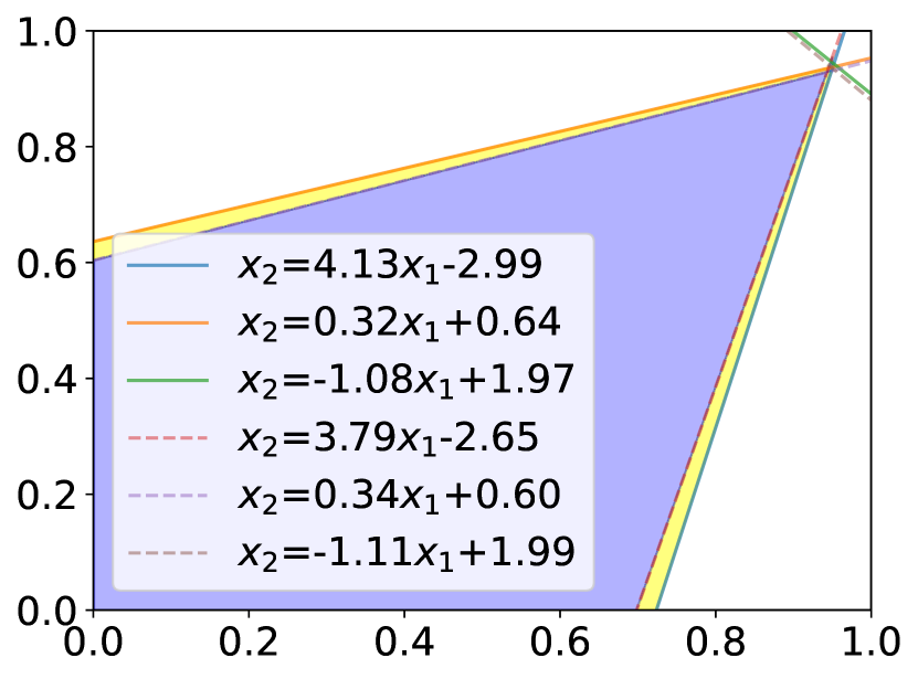
(b) After optimisation

Figure 7: Local optimisation for preimage under-approximation. The preimage polytope in blue in Figure 7(a) represents the under-approximation before optimisation. The yellow region in Figure 7(b) indicates the expanded polytope volume after optimisation.

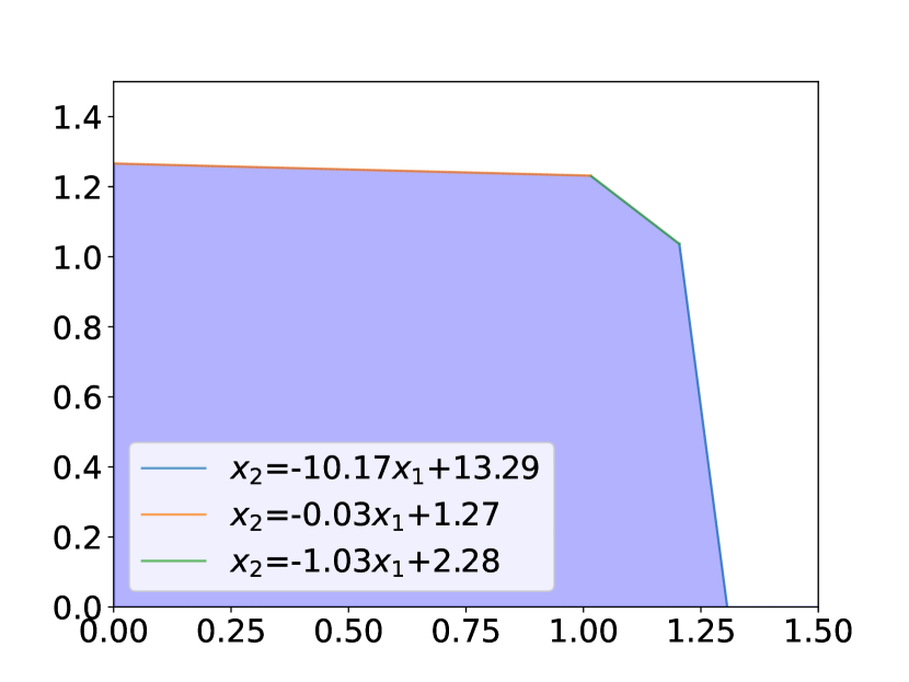
(a) No optimisation

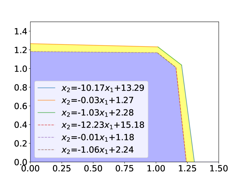
(b) After optimisation

Figure 8: Local optimisation for preimage over-approximation. The preimage polytope in blue represents the over-approximation before and after optimisation in Figure 8(a) and 8(b). The yellow region shows the reduced polytope volume after optimisation.

Example 5

We revisit Example 1. Figure 7(a) and 7(b) show the computed under-approximations before and after local optimisation. We can see that the bounding planes for all three specifications are optimised, such that the volume of the approximation has increased. Similarly, in Figure 8(a) and 8(b) we show the over-approximations before and after optimisation; it can be seen that the volume of the over-approximation has decreased.

4.5 Optimisation of Lagrangian Relaxation

Previously, in Section 4.3, we proposed a preimage refinement method that adds intermediate ReLU splitting planes to tighten the bounds of a selected individual neuron. However, intermediate bounds for other neurons are not updated based on the newly added splitting constraint. In the following, we first discuss the impact of stabilising an intermediate ReLU neuron from two different perspectives. We then present an optimisation approach leveraging Lagrangian relaxation to enforce the splitting constraint on refining the preimage.

Effect of Stabilisation of Intermediate Neurons. Our previous approach of Zhang et al. (2024) exploits one level of bound tightening after ReLU splitting: the substitution of relaxation functions with exact linear functions for the individual neuron. Specifically, assume an intermediate (unstable) neuron $z^{(i)}_{j}$ ($=h^{(i)}_{j}(x)$) is selected to split the input (sub)region $\mathcal{C}$ into two subregions $\mathcal{C}^{+}_{z^{(i)}_{j}}=\{x\in\mathcal{C}\leavevmode\nobreak\ |\leavevmode\nobreak\ z^{(i)}_{j}\geq 0\}$ and $\mathcal{C}^{-}_{z^{(i)}_{j}}=\{x\in\mathcal{C}\leavevmode\nobreak\ |\leavevmode\nobreak\ z^{(i)}_{j}<0\}$. For each subregion, the linear bounding functions of the nonlinear activation function $a^{(i)}_{j}(z^{(i)}_{j})$, as shown in Figure 2 (unstable mode), are then substituted with the exact ones, eliminating relaxation errors on the particular neuron. Another effect, potentially more impactful, is the bound tightening of every other intermediate neuron. Intuitively, one can tighten the intermediate bounds of (and thus stabilise) the other unstable neurons, since we are restricted to a smaller input region with the added splitting plane. A straightforward solution to enforce the effect of the splitting constraint is to call a regular LP solver to compute the new lower and upper bounds for every intermediate ReLU neuron under the splitting constraints. Naturally, this is computationally expensive ($2N$ LP calls where $N$ is the number of ReLU neurons).

Refinement with Optimisation of Lagrangian Relaxation. In order to derive tighter preimage approximations without explicitly introducing LP solver calls, we propose to adapt Lagrangian optimisation techniques (Wang et al., 2021b) to preimage generation. Consider first the case of generating under-approximations. Without loss of generality, we focus on preimage generation for the $k$-th output specification constraint, $\underline{g_{k}}(x)=\underline{a}_{k}^{T}x+\underline{b}_{k}$. We will drop the subscript $k$ for simplicity.

Consider the subregion where we have $z^{(i)}_{j}\leq 0$. To tighten the bounding plane $\underline{g}(x)$ of the preimage under the splitting constraint $z^{(i)}_{j}\leq 0$, we introduce the Lagrange multiplier, parameterized as $\beta^{(i)}_{j}(\geq 0)$, to enforce its effect throughout the neuron network. When propagating through layer $i$, we initially have:

$$g(\bm{z}^{(i)})\geq\bm{\underline{\textbf{A}}}^{(i)}\bm{z}^{(i)}+\underline{\textbf{b}}^{(i)}$$ (15)

Now, we add the splitting constraint using a Lagrange multiplier and obtain a Lagrangian relaxation of the original problem as follows:

$$g(\bm{z}^{(i)})\geq\max_{\beta^{(i)}_{j}\geq 0}\,\bm{\underline{\textbf{A}}}^{(i)}\bm{z}^{(i)}+\underline{\textbf{b}}^{(i)}+\beta^{(i)}_{j}z^{(i)}_{j}$$ (16)

Note that $\max_{\beta^{(i)}_{j}\geq 0}\beta^{(i)}_{j}z^{(i)}_{j}=0$, and thus Equation 16 holds in the universally quantified region. For the other case where $z^{(i)}_{j}\geq 0$, we can obtain a sound lower bound similarly by changing the sign for the additional splitting constraint:

$$g(\bm{z}^{(i)})\geq\max_{\beta^{(i)}_{j}\geq 0}\,\bm{\underline{\textbf{A}}}^{(i)}\bm{z}^{(i)}+\underline{\textbf{b}}^{(i)}-\beta^{(i)}_{j}z^{(i)}_{j}$$ (17)

We then propagate this backwards through the network to obtain a valid lower bound with respect to the input layer $x$:

$$g(x)\geq\underline{g}(x)=\max_{\bm{\beta}\geq 0}\,\underline{\textbf{A}}(\bm{\alpha},\bm{\beta})x+\underline{\textbf{b}}(\bm{\alpha},\bm{\beta})$$ (18)

Here, we explicitly note the dependence of the linear coefficients on $\bm{\beta}$, which denotes the vector of $\beta^{(i)}_{j}$ introduced for all split neurons. Once we obtain the bounding plane for each half-space constraint in $O$, the preimage polytope can be formulated as $T_{\mathcal{C}}(O)=\{x|\bigwedge_{i=1}^{K}\underline{g_{i}}(x,\bm{\alpha}_{i},\bm{\beta}_{i})\geq 0\wedge\bigwedge_{i=1}^{d}\phi_{i}(x)\}$.

Similarly to the optimisation over relaxation parameters $\bm{\alpha}$, we can then optimise $\bm{\beta}$ to maximise the preimage volume. Our differentiable preimage volume estimate is given by:

$$\widehat{\textnormal{vol}}(T_{\mathcal{C}_{sub},\bm{\alpha},\bm{\beta}}(O))=\frac{\text{vol}(\mathcal{C})}{N}\sum_{j=1}^{N}\sigma\left(-\textnormal{LSE}(-\underline{g_{1}}(x_{j},\bm{\alpha}_{1},\bm{\beta}_{1}),...,-\underline{g_{K}}(x_{j},\bm{\alpha}_{K},\bm{\beta}_{K}))\right)$$ (19)

where we have added the dependence on the Lagrange multipliers $\bm{\beta}$ to Equation 12. Intuitively, the additional splitting constraint enforced by the Lagrangian relaxation reduces the input space for maximising the preimage volume, which allows a tighter preimage bounding plane for the subregion. In the case where all $\bm{\beta}$ coefficients are zero, this corresponds precisely to the previous standard LiRPA bound with $\bm{\alpha}$ parameters from Section 4.4. We then maximise the volume estimate of the under-approximation with the following loss function in Algorithm 2 (Line 2):

$$\textnormal{Loss}(\bm{\alpha},\bm{\beta})=-\widehat{\textnormal{vol}}(\underline{T_{\mathcal{C}_{sub},\bm{\alpha},\bm{\beta}}}(O))$$ (20)

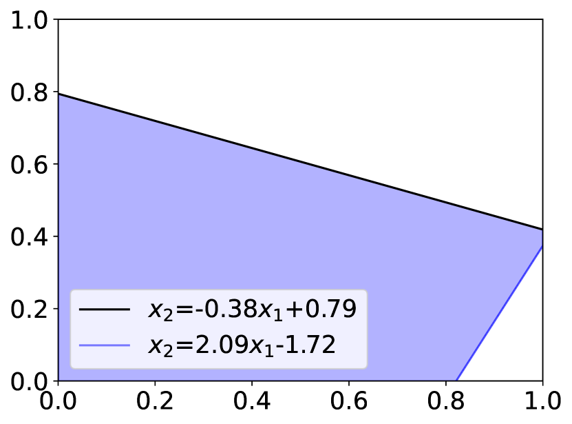
(a) Before optimisation

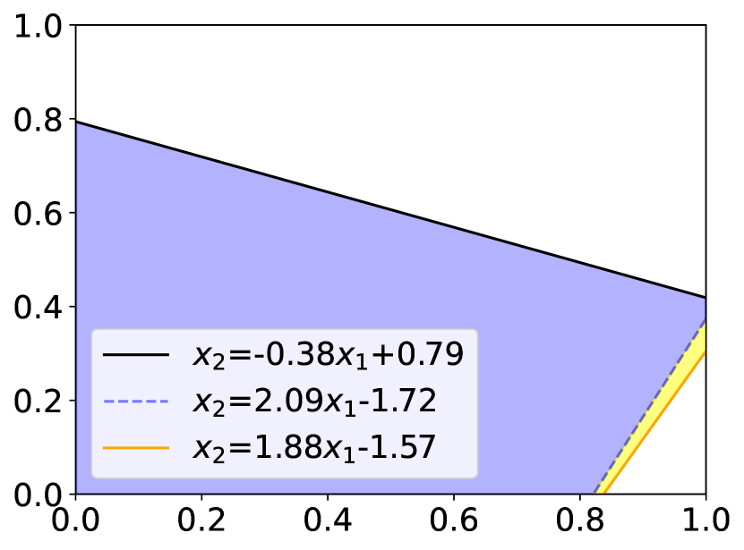
(b) After optimisation

Figure 9: Optimisation of Lagrangian relaxation for preimage refinement. The preimage polytope in blue represents the under-approximation before Lagrangian optimisation and the yellow region displays the expanded polytope after optimisation. Details in Example 6.

Example 6

We now apply our optimisation method over Lagrangian relaxation to Example 1. Figure 9(a) and 9(b) show the preimage polytope before and after Lagrangian optimisation, respectively, where the splitting plane of the selected unstable ReLU node is marked with a black solid line. Note that the preimage in Figure 9(a) is computed by removing the relaxation errors of the selected unstable ReLU node, where the symbolic upper/lower bounding functions are substituted with the exact linear functions. The preimage is further refined, as in Figure 9(b), by enforcing the added splitting constraint $z^{(i)}_{j}\leq 0$ for one subdomain throughout the neuron network, which allows tighter preimage approximation (vs tightening via stabilizing a single neuron in Figure 9(a)).

4.6 Overall Algorithm

Our overall preimage approximation method is summarised in Algorithm 1. It takes as input a neural network $f$, input region $\mathcal{C}$, output region $O$, target polytope volume threshold $v$ (a proxy for approximation precision), maximum number of iterations $R$, number of samples $N$ for statistical estimation, and Boolean variables indicating (i) whether to return an under-approximation or over-approximation and (ii) whether to use input or ReLU splitting, and returns a disjoint polytope union $\mathcal{T}_{\text{Dom}}$ representing a guaranteed under-approximation (or over-approximation) to the preimage.

The algorithm initiates and maintains a priority queue of (sub)regions according to Equation 7. The initialisation step (Lines 1-1) generates an initial polytope approximation of the whole region using Algorithm 2 (Sections 4.2, 4.4, 4.5), with priority calculated (CalcPriority) according to Equations 4, 6. Then, the preimage refinement loop (Lines 1-1) partitions a subregion in each iteration, with the preimage restricted to the child subregions then being re-approximated (Line 1-1). In each iteration, we choose the region to split (Line 1) and the splitting plane to cut on (Line 1 for input split and Line 1 for ReLU split), as detailed in Section 4.3. The preimage subregion queue is then updated by computing the priorities for each subregion by approximating their volume (Line 1). The loop terminates and the approximation is returned when the target volume threshold $v$ or maximum iteration limit $R$ is reached.

4.7 Quantitative Verification

We now show how to use our efficient preimage under-approximation method (Algorithm 1) to verify a given quantitative property $(I,O,p)$, where $O$ is a polyhedron, $I$ a polytope and $p$ the desired proportion threshold, summarised in Algorithm 3. Note that preimage over-approximation cannot be applied for sound quantitative verification as the approximation may contain false regions outside the true preimage. To simplify, assume that $I$ is a hyperrectangle, so that we can take $\mathcal{C}=I$. We discuss the case of general polytopes at the end of this section.

Input: Neural network $f$, Property $(I,O,p)$, Maximum iterations $R$

Output: Verification result $\in\{\textnormal{True, False, Unknown}\}$

1

2$\textnormal{vol}(I)\leftarrow\textnormal{EstimateVolume}(I)$;

$\mathcal{C}\leftarrow\textnormal{OuterBox}(I)$ ;

  // For general polytopes $I$

3 $\mathcal{T}\leftarrow\textnormal{InitialRun}(f,\mathcal{C},O)$;

4 while $\textnormal{Iterations}\leq R$ do

5       $\mathcal{T}\leftarrow\textnormal{Refine}(f,\mathcal{T},\mathcal{C},O)$;

6       if $\textnormal{EstimateVolume}(\mathcal{T})\geq p\times\textnormal{vol}(I)$ then

7             return True

8      if AllReLUSplit then

9             return False

10      

return Unknown

Algorithm 3 Quantitative Verification

We utilise Algorithm 1 by setting the volume threshold v to $p\times\textnormal{vol}(I)$, such that we have $\frac{\textnormal{vol}(\mathcal{T})}{\textnormal{vol}(I)}\geq p$ if the algorithm terminates before reaching the maximum number of iterations. If the final preimage polytope volume $\textnormal{vol}(\mathcal{T})\geq p\times\textnormal{vol}(I)$, then the property is verified. Otherwise, we continue running the preimage refinement. If the refinement loop has stabilised all ReLU neurons and the volume threshold is still not achieved, the property is falsified.

In Algorithm 3, InitialRun generates an initial under-approximation to the preimage as in Lines 1-1 of Algorithm 1, and Refine performs one iteration of approximation refinement (Lines 1-1). Termination occurs when we have verified or falsified the quantitative property, or when the maximum number of iterations has been exceeded.

Proposition 7

Algorithm 3 is sound for quantitative verification with input splitting.

Proposition 8

Algorithm 3 is sound and complete for quantitative verification on piecewise linear neural networks with ReLU splitting.

Proofs of the propositions are presented in Appendix B.

General Input Polytopes. Previously we detailed how to use our preimage under-approximation method to verify quantitative properties $(I,O,p)$, where $I$ is a hyperrectangle. We now discuss how to extend our method for a general polytope $I$.

Firstly, in Line 3 of Algorithm 3, we derive a hyperrectangle $\mathcal{C}$ such that $I\subseteq\mathcal{C}$, by converting the polytope $I$ into its V-representation (Grünbaum et al., 2003), that is, a list of the vertices (extreme points) of the polytope, which can be computed as in Avis and Fukuda (1991); Barber et al. (1996). Once we have a V-representation, obtaining a bounding box can be achieved simply by computing the minimum and maximum value $\underline{x_{i}},\overline{x_{i}}$ of each dimension among all vertices.

Once we have the input region $\mathcal{C}$, we can then run the preimage refinement as usual, but with the modification that, when defining the polytopes and restricted preimages, we must additionally include the polytope constraints from $I$. Practically, this means that, during every call to EstimateVolume in Algorithm 3, we add these polytope constraints, and in Line 2 of Algorithm 2 we add the polytope constraints from $I$, in addition to those derived from the output $O$ and the box constraints from $\mathcal{C}_{sub}$.

5 Experiments

We have implemented our approach as a tool for preimage approximation for polyhedral output sets/specifications. In this section, we report on experimental evaluation of the proposed approach, and demonstrate its effectiveness in approximation generation and the application to quantitative analysis of neural networks.

5.1 Benchmark and Evaluation Metric

We evaluate our preimage analysis approach on a benchmark of reinforcement learning and image classification tasks. Besides the vehicle parking task of Ayala et al. (2011) shown in the running example, we consider the following tasks: (1) aircraft collision avoidance system (VCAS) from Julian and Kochenderfer (2019) with 9 feed-forward neural networks (FNNs); (2) neural network controllers from Müller et al. (2022) for three reinforcement learning tasks (Cartpole, Lunarlander, and Dubinsrejoin) as in Brockman et al. (2016); and (3) the neural network from VNN-COMP 2022 for MNIST classification. Details of the benchmark tasks and neural networks are summarised in Appendix A.

Evaluation Metric. To evaluate the quality of the preimage approximation, we define the coverage ratio to be the ratio of volume covered by the approximation to the volume of the exact preimage, i.e., $\textnormal{cov}(\mathcal{T},f^{-1}_{\mathcal{C}}(O))\mathrel{\mathop{\mathchar 58\relax}}=\frac{\textnormal{vol}(\mathcal{T})}{\textnormal{vol}(f^{-1}_{\mathcal{C}}(O))}$. Note that this is a normalised measure for assessing the quality of the approximation, as used in Algorithm 3 when comparing with target coverage proportion $p$ for termination of the refinement loop. In practice, we use Monte Carlo estimation to compute $\textnormal{vol}(f^{-1}_{\mathcal{C}}(O))$ as $\widehat{\textnormal{vol}}(f^{-1}_{\mathcal{C}}(O))=\text{vol}(\mathcal{C})\times\frac{1}{N}\sum_{i=1}^{N}\mathds{1}_{f(x_{i})\in O}$, where $x_{1},...x_{N}$ are samples from $\mathcal{C}$. In Algorithm 1, the target volume (stopping criterion) is set as $v=r\times\widehat{\textnormal{vol}}(f^{-1}_{\mathcal{C}}(O)$, where $r$ is the target coverage ratio.

5.2 Evaluation

5.2.1 Effectiveness on Preimage Approximation with Input Split

Table 1: Performance comparison on preimage generation, for four different specifications on the vehicle parking task. Over-approximation results are highlighted with grey background in subcolumns labelled by ox, whereas under-approximation is shown with white background in subcolumns labelled by ux.

Vehicle Parking	Exact		Invprop				Our
	#Poly	Time(s)	Time(s)		Cov		#Poly		Time(s)		Cov
	exact	exact	ux	ox	ux	ox	ux	ox	ux	ox	ux	ox
$\wedge_{i\in\{2,3,4\}}y_{1}\geq y_{i}$	10	3110.979	2.642	0.907	0.921	1.043	4	4	1.116	1.121	0.957	1.092
$\wedge_{i\in\{1,3,4\}}y_{2}\geq y_{i}$	20	3196.561	2.242	0.793	0.895	1.051	4	4	1.235	1.336	0.948	1.074
$\wedge_{i\in\{1,2,4\}}y_{3}\geq y_{i}$	7	3184.298	2.325	0.865	0.906	1.083	3	4	1.074	1.129	0.952	1.098
$\wedge_{i\in\{1,2,3\}}y_{4}\geq y_{i}$	15	3206.998	2.402	0.793	0.915	1.058	3	3	1.055	1.004	0.922	1.061

We apply Algorithm 1 with input splitting to the preimage approximation problem for low-dimensional reinforcement learning tasks. For comparison, we also run the exact preimage generation method (Exact) from Matoba and Fleuret (2020) and the preimage over-approximation method (Invprop) from Kotha et al. (2023, accessed October, 2023).

Table 2: Performance comparison on preimage generation (average performance) on vehicle parking and VCAS, with over-approximation shown in grey background (subcolumns labelled by ox) and under-approximation in white background (subcolumns labelled by ux).

Tasks	Exact		Invprop				Our
	#Poly	Time(s)	Time(s)		Cov		#Poly		Time(s)		Cov
	exact	exact	ux	ox	ux	ox	ux	ox	ux	ox	ux	ox
Vehicle	13	3174.709	2.403	0.840	0.909	1.059	4	4	1.120	1.148	0.945	1.081
VCAS	131	6363.272	-	-	-	-	15	1	10.775	1.045	0.908	1.041

Vehicle Parking & VCAS. Table 1 and 2 present the comparison results with state-of-the-art exact and approximate preimage generation methods. In the table, we show the number of polytopes (#Poly) in the preimage, computation time (Time(s)), and the approximate coverage ratio (Cov) when the preimage approximation algorithm terminates with target coverage of 0.90 (the larger, the better) for under-approximation and 1.10 (the lower, the better) for over-approximation. Note that the Exact method computes the exact preimage (i.e., coverage ratio 1.0), while our method computes the under- and over-approximation of the exact preimage. The results for over-approximation are highlighted with grey background, whereas under-approximation is shown with white background. Invprop only supports computing over-approximations natively; thus, we adapt it to produce an under-approximation by computing over-approximations for the complement of each output constraint; note that the resulting approximation is then the complement of a union of polytopes, rather than a DUP.

Compared with the exact method, our approach yields orders-of-magnitude improvement in efficiency (see Table 1 and Table 2). It can also characterise the preimage with much fewer (and also disjoint) polytopes, achieving an average reduction of 69.2% for vehicle parking (both under- and over-approximation) and 88.5% (under-approximation) and 99.2% (over-approximation) for VCAS. Compared with Invprop, our method produces comparable results in terms of time and approximation coverage on the 2D vehicle parking task.

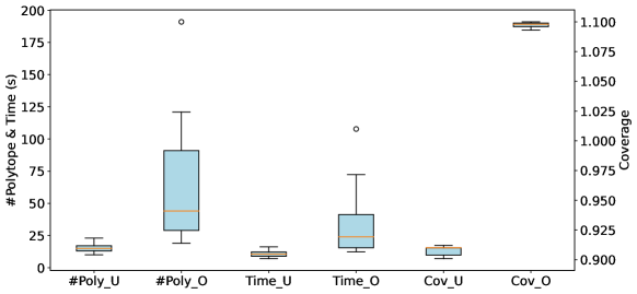
Figure 10: Preimage approximation results over the 9 VCAS neural networks. Results for under-approximation are indicated with metric_U and over-approximation with metric_O. The scale for both the number of polytopes and time is indicated on the vertical axis on the left.

While Table 2 shows average performance on VCAS, Figure 10 plots more detailed results of our method for the nine neural networks in the VCAS task in terms of the number of polytopes ($y$-axis on the left), time cost ($y$-axis on the left) and approximation coverage ($y$-axis on the right) for both under- (indicated with metric_U) and over-approximation (indicated with metric_O). As shown in the figure, our method is able to reach the targeted approximation coverage (0.90 for under-approximation and 1.10 for over-approximation) for all networks. The median number of polytopes for the preimage under-approximation for property $O=\{y\in\mathbb{R}^{9}\leavevmode\nobreak\ |\wedge_{i\in[1,9]}\leavevmode\nobreak\ y_{1}\geq y_{i}\}$ is 15 and the median time cost is 10.492s. The over-approximation shows higher variability in the number of generated polytopes and computation time for property $O=\{y\in\mathbb{R}^{9}\leavevmode\nobreak\ |\wedge_{i\in[1,9]\setminus 3}\leavevmode\nobreak\ y_{3}\geq y_{i}\}$, with the maximum reaching 191 polytopes and computation time of 107.758s for VCAS model 3.

Table 3: Performance of preimage approximation for reinforcement learning tasks, with over-approximation shown in grey background (marked in subcolumns ox) and under-approximation in white background (marked in subcolumns ux).

Task	Property	Config	#Poly		Cov		Time(s)
			ux	ox	ux	ox	ux	ox
Cartpole (FNN $2\times 64$)	$\{y\in\mathbb{R}^{2}|\leavevmode\nobreak\ y_{1}\geq y_{2}\}$	$\dot{\theta}\in[-2,-1]$	25	1	0.766	1.213	13.337	2.149
		$\dot{\theta}\in[-2,-0.5]$	42	8	0.750	1.242	19.732	5.778
		$\dot{\theta}\in[-2,0]$	66	22	0.755	1.246	30.563	11.476
Lunarlander (FNN $2\times 64$)	$\{y\in\mathbb{R}^{4}|\wedge_{i\in\{1,3,4\}}y_{2}\geq y_{i}\}$	$\dot{v}\in[-1,0]$	18	1	0.754	1.068	14.453	2.381
		$\dot{v}\in[-2,0]$	67	23	0.751	1.246	48.455	19.210
		$\dot{v}\in[-4,0]$	97	90	0.751	1.249	76.234	72.285
Dubinsrejoin (FNN $2\times 256$)	$\{y\in\mathbb{R}^{8}|\wedge_{i\in[2,4]}\leavevmode\nobreak\ y_{1}\geq y_{i}$ $\quad\quad\quad\,\bigwedge\wedge_{i\in[6,8]}\leavevmode\nobreak\ y_{5}\geq y_{i}\}$	$x_{v}\in[-0.1,0.1]$	211	20	0.751	1.242	182.821	18.666
		$x_{v}\in[-0.2,0.2]$	409	23	0.750	1.241	323.839	24.788
		$x_{v}\in[-0.3,0.3]$	677	43	0.750	1.244	589.939	41.502

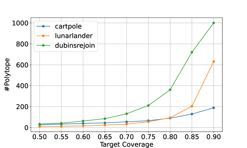
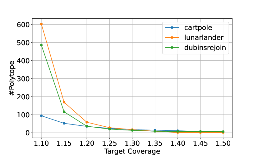
Figure 11: Number of polytopes in preimage approximation for a range of target coverage values. Left: under-approximation. Right: over-approximation.

Neural Network Controllers. In this experiment, we consider preimage approximation for neural network controllers in reinforcement learning tasks. Note that the Exact method in Matoba and Fleuret (2020) is unable to deal with neural networks of these sizes and Invprop in Kotha et al. (2023) is not capable of characterising the preimage under-approximation in the form of disjoint polytopes. Table 3 summarises the experimental results obtained by our method, where the columns for over-approximations are marked with grey background and under-approximations marked with a white background.

We evaluate Algorithm 1 (with input splitting) with respect to a range of different configurations of the input region (e.g., angular velocity $\dot{\theta}$ for Cartpole). For comparison, we set the same target coverage ratio for different input region sizes (0.75 for under-approximation and 1.25 for over-approximation) and an iteration limit of 1000. In Table 3, we see that our method successfully generates preimage approximations for all configurations, reaching the targeted approximation coverage. Empirically, for the same coverage ratio, our method requires a number of polytopes and time roughly linear in the input region size for the preimage under-approximation. For over-approximations, the bounding constraints of the input region are added as additional constraints to form the polytope approximation on each subregion, which affects the linear trend in the number of polytopes and computation time as the input region size increases. For example, the constraint brought by the input configuration of $-2\leq\dot{\theta}\leq-1$ for Cartpole, together with the single polytope over-approximation, already reaches the target coverage, while for a larger input region of $-2\leq\dot{\theta}\leq 0$, 22 preimage polytopes are needed together with input bounding constraints for each input subregion.

In Figure 11, we show the number of polytopes needed to reach different target coverage ratios for both under-approximation (left) and over-approximation (right). Our evaluation results indicate that the number of refinement iterations taken is influenced by the number of output constraints and the size of the neural network. For instance, the neural network controller for Cartpole, which has a single output constraint, shows a roughly linear increase in the number of polytopes as the target coverage increases for under-approximation (resp. decreases for over-approximation). In contrast, accommodating multiple output constraints for larger neural networks, e.g., Dubinsrejoin, requires a significant increase in refinement iterations as the target coverage approaches 1.

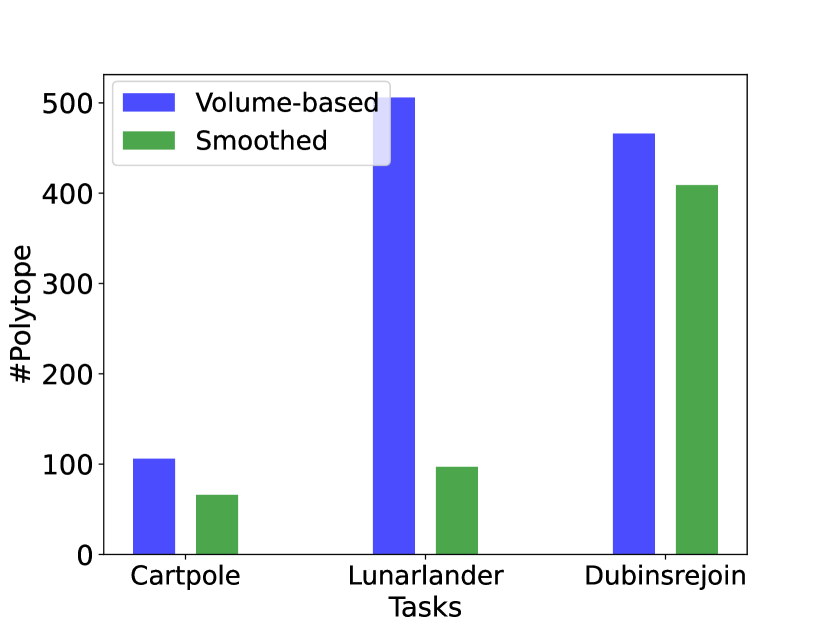
(a) Number of polytopes

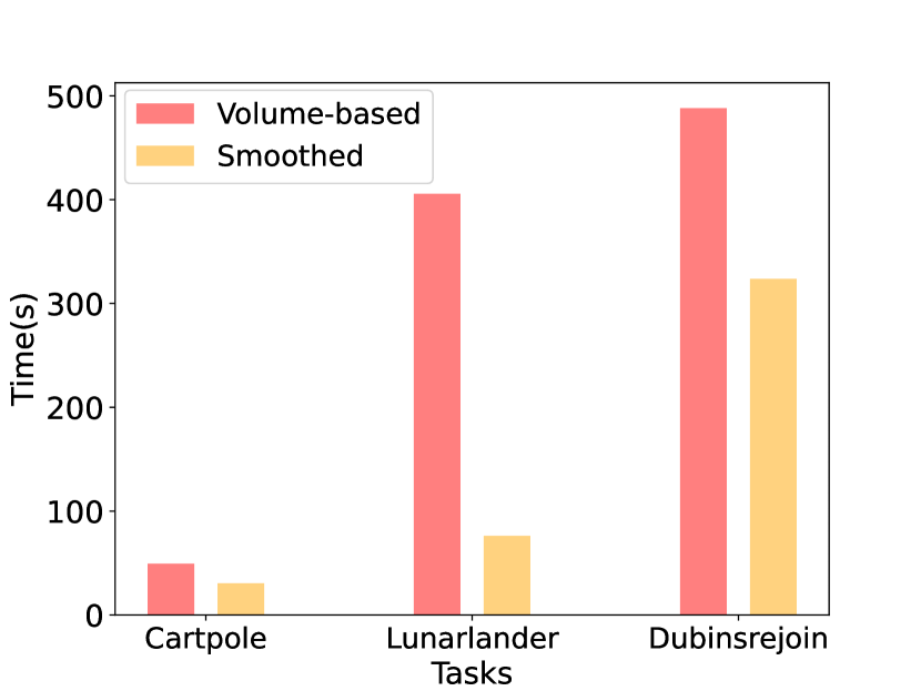
(b) Time cost

Figure 12: Effectiveness of smooth splitting for preimage under-approximation. Baseline method from Zhang et al. (2024).

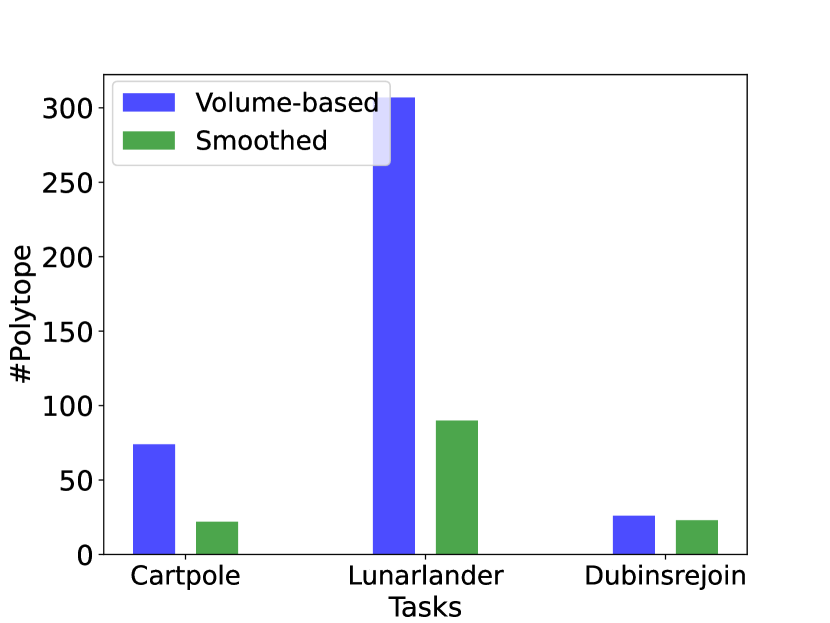
(a) Number of polytopes

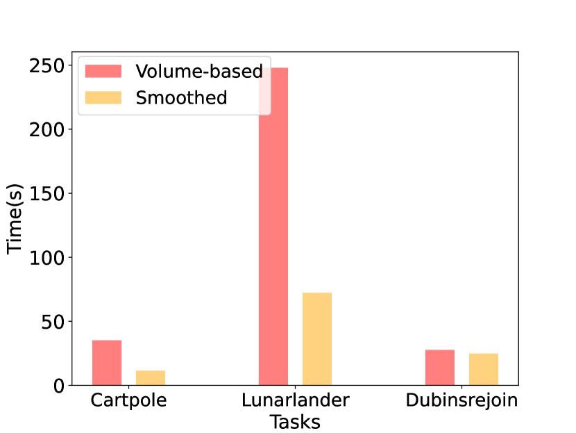
(b) Time cost

Figure 13: Effectiveness of smooth splitting for preimage over-approximation.

5.2.2 Effectiveness of Smoothed Input Splitting

We now analyse the effectiveness of the smoothed splitting method described in Section 4.3 (Equation 7 and 8), in comparison to a volume-guided splitting method that chooses the input feature leading to the greatest improvement in approximation volume. From Figures 12 and 13, we observe that the smoothed splitting method requires significantly fewer refinement iterations for all reinforcement learning controllers to achieve the target coverage, thus reducing the number of polytopes and computation time, than the volume-guided splitting method. More specifically, the smoothed splitting method achieves an average reduction of 43.6% in the number of polytopes and 51.0% in computation time for under-approximation across the neural network controllers, up to 80.8%/81.2% reduction for the Lunarlander task. Similar improvements in computation efficiency and size of polytope union are also achieved for over-approximations, with an average reduction of 50.8%/49.6% across all reinforcement learning tasks.

Recall that the smoothed input splitting heuristic relaxes the volume-based heuristic, such that, for each sampled input point in the input region, we take into account not only whether the point lies in the polytope approximation, but also how far away the point is from the approximation. This is particularly crucial in early iterations, where the approximation may be too loose; for example, an under-approximation may have no overlap with the input region (thus zero volume). Therefore, computing the approximation volume (after splitting on each input feature) provides very little signal. In such cases, the smoothed splitting heuristic is able to capture promising input features that, while not immediately improving the approximation volume, can bring the preimage bounding planes closer to the exact preimage, which is beneficial for future iterations.

5.2.3 Effectiveness of Preimage Approximation with ReLU Split

Table 4: Preimage under-approximation refinement with ReLU split ($L_{\infty}$ attack). Results with Lagrangian optimisation are marked in grey background in columns w/ LagOpt.

$L_{\infty}$ attack (FNN $6\times 100$)	#Poly		Cov		Time(s)
	w/o	w/ LagOpt	w/o	w/ LagOpt	w/o	w/ LagOpt
0.06	2	2	1.0	1.0	3.183	3.237
0.07	247	40	0.752	0.756	130.746	29.019
0.08	522	290	0.751	0.751	305.867	218.455
0.09	733	563	0.165	0.751	507.116	365.552

Table 5: Preimage under-approximation refinement with ReLU split (patch attack). Results with Lagrangian optimisation are marked in grey background in columns w/ LagOpt.

Patch attack (FNN $6\times 100$)	#Poly		Cov		Time(s)
	w/o	w/ LagOpt	w/o	w/ LagOpt	w/o	w/ LagOpt
$3\times 3$(center)	1	1	1.0	1.0	2.611	2.637
$4\times 4$(center)	678	678	0.382	0.427	455.988	514.272
$7\times 7$(corner)	7	7	0.842	0.861	6.065	6.217
$8\times 7$(corner)	956	954	0.033	0.214	488.849	676.666

In this subsection, we evaluate the scalability of Algorithm 1 with ReLU splitting by applying it to MNIST image classifiers. In particular, we consider input regions defined by bounded perturbations to a given MNIST image. Table 4 and 5 summarise the evaluation results for two types of image perturbations commonly considered in the adversarial robustness literature ($L_{\infty}$ and patch attack, respectively). For $L_{\infty}$ attacks, bounded perturbation noise is applied to all image pixels. The patch attack applies only to a smaller patch area of $n\times m$ pixels but allows arbitrary perturbations covering the whole valid range $[0,1]$. The task is then to produce a DUP approximation of the subset of the perturbation region that is guaranteed to be classified correctly.

For $L_{\infty}$ attack, we evaluate our method over perturbations of increasing size, from $0.06$ to $0.09$. It is worth noting that for this size of preimage, e.g., from $0.06$ to $0.07$, the volume of the input region increases by tens of orders of magnitude due to the high dimensionality, making effective preimage approximation significantly more challenging. Table 4 shows that our approach (Algorithm 1) without Lagrangian optimisation (marked in columns w/o) is able to generate a preimage under-approximation that achieves the targeted coverage of $0.75$ for $L_{\infty}$ noise up to 0.08. The fact that the number of polytopes and computation time remain manageable is due to the effectiveness of ReLU splitting. In Table 5, for the patch attack, we observe that the number of polytopes and time required increase sharply when increasing the patch size for both the centre and corner area of the image, suggesting that the model is more sensitive to larger local perturbations. It is also interesting that our method can generate preimage approximations for larger patches in the corner as opposed to the centre of the image; we hypothesize this is due to the greater influence of central pixels on the neural network output, and correspondingly a greater number of unstable neurons over the input perturbation space.

Table 6 shows the preimage refinement results for over-approximations in the context of patch attack. The results of our approach (Algorithm 1) without Lagrangian optimisation are summarised in columns w/o. As shown in the table, our refinement method can effectively tighten the over-approximation to the targeted coverage of 1.25 for different attack configurations. For patch size $10\times 10$ (centre) and $16\times 15$ (corner), we found that the perturbation region is a trivial over-approximation itself for the target coverage of 1.25; thus, we demonstrate the results with a target coverage of 1.1 and 1.05. Similarly to under-approximations, a patch attack in the centre with a smaller patch size requires more refinement iterations than the patch attack in the corner, demonstrating a greater influence of central pixels.

Effectiveness of Lagrangian Optimisation. The results of evaluation of our approach (Algorithm 1) for under-approximation with Lagrangian optimisation are shown in Table 4 and 5 (marked in columns w/ LagOpt with grey background). For $L_{\infty}$ attack, the refinement method with Lagrangian optimisation generates preimage approximations that achieve the target coverage of 0.75 for all perturbation settings, including perturbation noise $0.09$ where the refinement without Lagrangian optimisation fails (0.751 vs 0.165 in Table 4). The new refinement method also leads to a significant reduction in the number of polytopes and computation cost. For the patch attack, the refinement method with Lagrangian optimisation effectively improves the preimage approximation precision for all configuration settings. Since the patch attack allows arbitrary perturbations covering the whole valid range $[0,1]$, it leads to a rapid increase in the number of unstable neurons and exhausts the iteration limit when increasing the patch size. Nonetheless, the resulting preimage approximation coverage obtained with Lagrangian optimisation shows better per-iteration precision improvement, while introducing marginal computation overhead compared to the previous method.

Table 6: Preimage over-approximation refinement with ReLU split (patch attack). Results with Lagrangian optimisation are marked in grey background in columns w/ LagOpt.

Patch attack (FNN $6\times 100$)	#Poly		Cov		Time(s)
	w/o	w/ LagOpt	w/o	w/ LagOpt	w/o	w/ LagOpt
$10\times 10$(center)	387	387	1.099	1.099	261.826	281.916
$11\times 11$(center)	317	317	1.249	1.249	192.954	212.735
$16\times 15$(corner)	616	616	1.050	1.050	328.589	350.092
$16\times 16$(corner)	285	285	1.249	1.249	165.250	175.605

Columns w/ LagOpt in Table 6 summarises the over-approximation results with Lagrangian optimisation. In this case, we introduce the Lagrange multipliers with the opposite signs to the under-approximation to guarantee the validity of the symbolic over-approximation. Intriguingly, in contrast to under-approximation, we find that the optimised $\beta$ parameters are almost always close to 0, meaning that the results are similar to not using Lagrangian optimisation. We hypothesize that, for over-approximations, the objective function is relatively flat in the vicinity of $0$, which makes the parameters difficult to optimise.

Table 7: Comparison with a robustness verifier.

Task	$\alpha,\beta$-CROWN		Our
	Result	Time	Cov(%)	#Poly	Time
Cartpole ($\dot{\theta}\in[-1.642,-1.546]$)	yes	3.349	100.0	1	1.137
Cartpole ($\dot{\theta}\in[-1.642,0]$)	no	6.927	94.9	2	3.632
MNIST ($L_{\infty}$ 0.026)	yes	3.415	100.0	1	2.649
MNIST ($L_{\infty}$ 0.04)	unknown	267.139	100.0	2	3.019

Comparison with Robustness Verifiers. We now illustrate empirically the utility of preimage computation in robustness analysis compared to robustness verifiers. Table 7 shows comparison results with $\alpha,\beta$-CROWN, winner of the VNN competition (Müller et al., 2022). We set the tasks according to the problem instances from VNN-COMP 2022 for local robustness verification (localised perturbation regions). For Cartpole, $\alpha,\beta$-CROWN can provide a verification guarantee (yes/no or safe/unsafe) for both problem instances. However, in the case where the robustness property does not hold, our method explicitly generates a preimage under-approximation in the form of a disjoint polytope union (which guarantees the satisfaction of the output properties), and covers $94.9\%$ of the exact preimage. For MNIST, while the smaller perturbation region is successfully verified, $\alpha,\beta$-CROWN with tightened intermediate bounds by MIP solvers returns unknown with a timeout of 300s for the larger region. In comparison, our algorithm provides a concrete union of polytopes where the input is guaranteed to be correctly classified, which we find covers 100$\%$ of the input region (up to sampling error). Note also, as shown in Table 4, our algorithm can produce non-trivial under-approximations for input regions far larger than $\alpha,\beta$-CROWN can verify.

5.2.4 Quantitative Verification

We now demonstrate the application of our preimage under-approximation to quantitative verification of the property $(I,O,p)$; that is, we aim to check whether $f(x)\in O$ for at least proportion $p$ of input values $x\in I$. Table 8 summarises the quantitative verification results, which leverage the disjointness of our under-approximation, such that we can compute the total volume covered by computing the volume of each individual polytope.

Vertical Collision Avoidance System. In this example, we consider the VCAS system and a scenario where the two aircraft have negative relative altitude from intruder to ownship ($h\in[-8000,0]$), the ownship aircraft has a positive climbing rate $\dot{h_{A}}\in[0,100]$ and the intruder has a stable negative climbing rate $\dot{h_{B}}=-30$, and time to the loss of horizontal separation is $t\in[0,40]$, which defines the input region $I$. For this scenario, the correct advisory is “Clear Of Conflict” (COC). We apply Algorithm 3 to verify the quantitative property where $O=\{y\in\mathbb{R}^{9}|\bigwedge_{i=2}^{9}y_{1}-y_{i}\geq 0\}$ and the proportion $p=0.9$, with an iteration limit of 1000. The quantitative proportion reached by the generated under-approximation is 90.8%, which verifies the quantitative property in 5.620s.

Table 8: Quantitative verification results with preimage under-approximation.

Task	Property	#Poly	Time(s)	QuantProp(%)
VCAS	$O=\{y\in\mathbb{R}^{9}|\bigwedge_{i=2}^{9}y_{1}-y_{i}\geq 0\}$	6	5.620	90.8
Cartpole	$O=\{y|y_{1}-y_{2}\geq 0\}$	11	12.1	90.0
Lunarlander	$O=\{y\in\mathbb{R}^{4}|\wedge_{i\in\{1,3,4\}}y_{2}\geq y_{i}\}$	120	429.480	90.0

Cartpole. In the Cartpole problem, the objective is to balance the pole attached to a cart by pushing the cart either left or right. We consider a scenario where the cart position is to the right of the centre ($x\in[0,1]$), the cart is moving right ($\dot{x}\in[0,0.5]$), the pole is slightly tilted to the right ($\theta\in[0,0.1]$) and pole is moving to the left ($\dot{\theta}\in[-0.2,0]$). To balance the pole, the neural network controller needs to determine “pushing left”. We apply Algorithm 3 to verify the quantitative property, where $O=\{y|y_{1}-y_{2}\geq 0\}$ and the proportion $p=0.9$, with an iteration limit of 1000. The under-approximation algorithm takes 12.1s to reach the target proportion 90.0%.

Lunarlander. In the Lunarlander task, the objective of the neural networks controller is to achieve a safe landing of the lander. Consider a scenario where the lander is slightly to the left of the centre of the landing pad ($x\in[-1,0]$), the lander is above the landing pad sufficient for descent correction ($h\in[0,1]$), and it is moving to the right ($\dot{x}\in[1,2]$) but descending rapidly ($\dot{h}\in[-2,-1]$). To avoid a hard landing, the neural network controller needs to reduce the descent speed by taking the action “fire main engine”. We formulate the quantitative property for this task, where $O=\{y\in\mathbb{R}^{4}|\wedge_{i\in\{1,3,4\}}y_{2}\geq y_{i}\}$ and the proportion $p=0.9$. To compute preimage under-approximation for this more complex task takes 429.480s to reach the target proportion 90.0%.

6 Related Work

Our paper is related to a series of works on robustness verification of neural networks. To address the scalability issues with complete verifiers (Huang et al., 2017; Katz et al., 2017; Tjeng et al., 2019) based on constraint solving, convex relaxation (Salman et al., 2019) has been used for developing highly efficient incomplete verification methods (Zhang et al., 2018; Wong and Kolter, 2018; Singh et al., 2019; Xu et al., 2020). Later works employed the branch-and-bound (BaB) framework (Bunel et al., 2018, 2020) to achieve completeness, using incomplete methods for the bounding procedure (Xu et al., 2021; Wang et al., 2021b; Ferrari et al., 2022). In this work, we adapt convex relaxation for efficient preimage approximation. Further, our divide-and-conquer procedure is analogous to BaB, but focuses on maximising covered volume for under-approximation (resp. minimising for over-approximation) rather than maximising or minimising a function value. There are also works that have sought to define a weaker notion of local robustness known as statistical robustness (Webb et al., 2019b; Mangal et al., 2019; Wang et al., 2021a), which requires that a proportion of points under some perturbation distribution around an input point are classified in the same way. Verification of statistical robustness is typically achieved by sampling and statistical guarantees (Webb et al., 2019b; Baluta et al., 2021; Tit et al., 2021; Yang et al., 2021). In this paper, we apply our symbolic approximation approach to quantitative analysis of neural networks, while providing exact quantitative rather than statistical evaluation (Webb et al., 2019a).

Another line of related works considers deriving exact or approximate abstractions of neural networks, which are applied for explanation (Sotoudeh and Thakur, 2021), verification (Elboher et al., 2020; Pulina and Tacchella, 2010), reachability analysis (Prabhakar and Afzal, 2019), and preimage approximation (Dathathri et al., 2019; Kotha et al., 2023). Dathathri et al. (2019) leverages symbolic interpolants (Albarghouthi and McMillan, 2013) for preimage approximations, facing exponential complexity in the number of hidden neurons. Kotha et al. (2023) considers the preimage overapproximation problem via inverse bound propagation, but their approach cannot be directly extended to the under-approximation setting. They also do not consider any strategic branching and refinement methodologies like those in our unified framework. Our anytime algorithm, which combines convex relaxation with principled splitting strategies for refinement, is applicable for both under- and over-approximations. Their work may benefit from our splitting strategies to scale to higher dimensions.

7 Conclusion

We present an efficient and unifying algorithm for preimage approximation of neural networks. Our anytime method derives from the observation that linear relaxation can be used to efficiently produce approximations, in conjunction with custom-designed strategies for iteratively decomposing the problem to rapidly improve the approximation quality. We formulate the preimage approximation in each refinement iteration as an optimisation problem and propose a differentiable objective to derive tighter preimages via optimising over convex bounding parameters and Lagrange multipliers. Unlike previous approaches, our method is designed for, and scales to, both low and high-dimensional problems. Experimental evaluation on a range of benchmark tasks shows significant advantages in runtime efficiency and scalability, and the utility of our method for important applications in quantitative verification and robustness analysis.

Acknowledgments and Disclosure of Funding

This project received funding from the ERC under the European Union’s Horizon 2020 research and innovation programme (FUN2MODEL, grant agreement No. 834115) and ELSA: European Lighthouse on Secure and Safe AI project (grant agreement No. 101070617 under UK guarantee). This work was done in part while Benjie Wang was visiting the Simons Institute for the Theory of Computing.

Appendix A Experiment Setup

In this section, we present the detailed configuration of neural networks in the benchmark tasks.

A.1 Vehicle Parking.

For the vehicle parking task, we train a neural network with one hidden layer of 20 neurons, which is computationally feasible for exact preimage computation for comparison. We consider computing the preimage approximation with input region corresponding to the entire input space $\mathcal{C}=\{x\in\mathbb{R}^{2}|x\in[0,2]^{2}\}$, and output sets $O_{k}$, which correspond to the neural network outputting label $k$: $O_{k}=\{y\in\mathbb{R}^{4}\leavevmode\nobreak\ |\bigwedge_{i\in\{1,2,3,4\}\setminus k}y_{k}-y_{i}\geq 0\},\quad k\in\{1,2,3,4\}$.

A.2 Aircraft Collision Avoidance

The aircraft collision avoidance (VCAS) system (Julian and Kochenderfer, 2019) is used to provide advisory for collision avoidance between the ownship aircraft and the intruder. VCAS uses four input features $(h,\dot{h_{A}},\dot{h_{B}},t)$ representing the relative altitude of the aircrafts, vertical climbing rates of the ownship and intruder aircrafts, respectively, and time to the loss of horizontal separation. VCAS is implemented by nine feed-forward neural networks built with a hidden layer of 21 neurons. In our experiment, we use the following input region for the ownship and intruder aircraft as in Matoba and Fleuret (2020): $h\in[-8000,8000]$, $\dot{h_{A}}\in[-100,100]$, $\dot{h_{B}}=30$, and $t\in[0,40]$. In the training, the input configurations are normalized into a range of $[-1,1]$. We consider the output property $O=\{y\in\mathbb{R}^{9}\leavevmode\nobreak\ |\wedge_{i\in[2,9]}\leavevmode\nobreak\ y_{1}\geq y_{i}\}$ and generate the preimage approximation for the VCAS neural networks.

A.3 Neural Network Controllers

A.3.1 Cartpole

The cartpole control problem considers balancing a pole atop a cart by controlling the movement of the cart. The neural network controller has two hidden layers with 64 neurons, and uses four input variables representing the position and velocity of the cart, the angle and angular velocity of the pole. The controller outputs are pushing the cart left or right. In the experiments, we set the following input region for the Cartpole task: (1) cart position $[-1,1]$, (2) cart velocity $[0,2]$, (3) angle of the pole $[-0.2,0]$, and (4) angular velocity of the pole $[-2,0]$ (with varied feature length in the evaluation). We consider the output property for the action pushing left.

A.3.2 Lunarlander

The Lunarlander problem considers the task of correct landing of a moon lander on a landing pad. The neural network for Lunarlander has two hidden layers with 64 neurons, and eight input features addressing the lander’s coordinate, orientation, velocities, and ground contact indicators. The outputs represent four actions. For the Lunarlander task, we set the input region as: (1) horizontal and vertical position $[-1,0]$ $\times$ $[0,1]$, (2) horizontal and vertical velocity $[0,2]$ $\times$ $[-2,0]$ (with varied feature length for evaluation), (3) angle and angular velocity $[-1,0]\times[-0.1,0.1]$, (4) left and right leg contact $[0.9,1]^{2}$. We consider the output specification for the action “fire main engine”, i.e., $\{y\in\mathbb{R}^{4}\leavevmode\nobreak\ |\wedge_{i\in\{1,3,4\}}y_{2}\geq y_{i}\}$.

A.3.3 Dubinsrejoin.

The Dubinsrejoin problem considers guiding a wingman craft to a certain radius around a lead aircraft. The neural network controller has two hidden layers with 256 neurons. The input space of the neural network controller is eight-dimensional, with the input variables capturing the position, heading, velocity of the lead and wingman crafts, respectively. The outputs are also eight dimensional representing controlling actions of the wingman. Note that the eight neural network outputs are processed further as tuples of actuators (rudder, throttle) for controlling the wingman where each actuator has 4 options. The control action tuple is decided by taking the action with the maximum output value among the first four network outputs (the first actuator options) and the action with the maximum value among the second four network outputs (the second actuator options). In the experiments, we set the following input region: (1) horizontal and vertical position $[-0.2,0]\times[0,0.5]$, (2) heading and velocity $[-1,0]\times[0,0.2]$ for the lead aircraft, and (3) horizontal and vertical position $[0.4,0.6]\times[-0.3,0.3]$ (with varied feature length for evaluation), (4) heading and velocity $[0.2,0.5]\times[-0.5,0.5]$ for the wingman aircraft. We consider the output property that both actuators (rudder, throttle) take the first option, i.e., $\{y\in\mathbb{R}^{8}\leavevmode\nobreak\ |\wedge_{i\in\{2,3,4\}}\leavevmode\nobreak\ y_{1}\geq y_{i}\bigwedge\wedge_{i\in\{6,7,8\}}\leavevmode\nobreak\ y_{5}\geq y_{i}\}$.

A.4 MNIST Classification

We use the trained neural network from VNN-COMP 2022 (Müller et al., 2022) for digit image classification. The neural network has six layers with a hidden neuron size of 100 for each hidden layer. We consider two types of image attacks: $l_{\infty}$ and patch attack. For $L_{\infty}$ attack, a perturbation is applied to all pixels of the image. For the patch attack, it applies arbitrary perturbations to the patch area, i.e., the perturbation noise covers the whole valid range $[0,1]$, for which we set the patch area at the centre and (upper-left) corner of the image with different sizes.

Appendix B Proofs

We present the propositions and proofs on guaranteed polytope volume improvement with each refinement iteration, noting that these propositions are valid without stochastic optimisation. Subsequently, we provide proofs for Propositions 7 and 8.

Proposition 9

Given any subregion $\mathcal{C}_{sub}$ with polytope under-approximation $T_{\mathcal{C}_{sub}}(O)$, and its children $\mathcal{C}_{sub}^{l},\mathcal{C}_{sub}^{u}$ with polytope under-approximations $T_{\mathcal{C}_{sub}^{l}}(O),T_{\mathcal{C}_{sub}^{u}}(O)$ respectively, it holds that:

$$T_{\mathcal{C}_{sub}^{l}}(O)\cup T_{\mathcal{C}_{sub}^{u}}(O)\supseteq T_{\mathcal{C}_{sub}}(O)$$ (22)

Proof  We define $T_{\mathcal{C}_{sub}}(O)|_{l},T_{\mathcal{C}_{sub}}(O)|_{r}$ to be the restrictions of $T_{\mathcal{C}_{sub}}(O)$ to $\mathcal{C}_{sub}^{l}$ and $\mathcal{C}_{sub}^{r}$ respectively, that is:

$$T_{\mathcal{C}_{sub}}(O)|_{l}=\{x\in\mathbb{R}^{d}|\bigwedge_{i=1}^{K}(\underline{g_{i}}(x)\geq 0)\wedge(x\in\mathcal{C}_{sub}^{l})\}$$ (23)

$$T_{\mathcal{C}_{sub}}(O)|_{r}=\{x\in\mathbb{R}^{d}|\bigwedge_{i=1}^{K}(\underline{g_{i}}(x)\geq 0)\wedge(x\in\mathcal{C}_{sub}^{r})\}$$ (24)

where we have replaced the constraint $x\in\mathcal{C}_{sub}$ with $x\in\mathcal{C}_{sub}^{l}$ (resp. $x\in\mathcal{C}_{sub}^{r}$), and $\underline{g_{i}}(x)$ is the LiRPA lower bound for the $i^{\textnormal{th}}$ specification on the input region $\mathcal{C}_{sub}$.

On the other hand, we also have:

$$T_{\mathcal{C}_{sub}^{l}}(O)=\{x\in\mathbb{R}^{d}|\bigwedge_{i=1}^{K}(\underline{g_{l,i}}(x)\geq 0)\wedge(x\in\mathcal{C}_{sub}^{l})\}$$ (25)

$$T_{\mathcal{C}_{sub}^{r}}(O)=\{x\in\mathbb{R}^{d}|\bigwedge_{i=1}^{K}(\underline{g_{r,i}}(x)\geq 0)\wedge(x\in\mathcal{C}_{sub}^{r})\}$$ (26)

where $\underline{g_{l,i}}(x)$ (resp. $\underline{g_{r,i}}(x)$) is the LiRPA lower bound for the $i^{\textnormal{th}}$ specification on the input region $\mathcal{C}_{sub}^{l}$ (resp. $\mathcal{C}_{sub}^{r}$). Now, it is sufficient to show that $T_{\mathcal{C}_{sub}^{l}}(O)\supseteq T_{\mathcal{C}_{sub}}(O)|_{l}$ and $T_{\mathcal{C}_{sub}^{r}}(O)\supseteq T_{\mathcal{C}_{sub}}(O)|_{r}$ to prove Equation 22. We will now show that $T_{\mathcal{C}_{sub}^{l}}(O)\supseteq T_{\mathcal{C}_{sub}}(O)|_{l}$ (the proof for $T_{\mathcal{C}_{sub}^{r}}(O)\supseteq T_{\mathcal{C}_{sub}}(O)|_{r}$ is entirely similar).

Before proving this result in full, we outline the approach and a sketch proof. It suffices to prove (for all $i$) that $\underline{g_{l,i}}(x)$ is a tighter bound than $\underline{g_{i}}(x)$ on $\mathcal{C}_{sub}^{l}$. That is, to show that $\underline{g_{l,i}}(x)\geq\underline{g_{i}}(x)$ for inputs $x$ in $\mathcal{C}_{sub}^{l}$, as then $\underline{g_{i}}(x)\geq 0\implies\underline{g_{l,i}}(x)\geq 0$ for inputs $x$ in $\mathcal{C}_{sub}^{l}$, and so $T_{\mathcal{C}_{sub}^{l}}(O)\supseteq T_{\mathcal{C}_{sub}}(O)|_{l}$. The bound $\underline{g_{l,i}}(x)$ is tighter than $\underline{g_{i}}(x)$ because the input region for LiRPA is smaller for $\underline{g_{l,i}}(x)$, leading to tighter concrete neuron bounds, and thus tighter bound propagation through each layer of the neural network $g_{i}$. We present the formal proof of greater bound tightness for input and ReLU splitting in the following.

Input split: We show $\underline{g_{l,i}}(x)\geq\underline{g_{i}}(x)$ for all $x\in\mathcal{C}_{sub}^{l}$ by induction (dropping the index $i$ in the following as it is not important). Recall that LiRPA generates symbolic upper and lower bounds on the pre-activation values of each layer in terms of the input (i.e. treating that layer as output), which can then be converted into concrete bounds.

$$\underline{\textbf{A}}^{(j)}x+\underline{\textbf{b}}^{(j)}\leq h^{(j)}(x)\leq\overline{\textbf{A}}^{(j)}x+\overline{\textbf{b}}^{(j)}$$ (27)

$$\underline{\textbf{A}}^{(l,j)}x+\underline{\textbf{b}}^{(l,j)}\leq h^{(j)}(x)\leq\overline{\textbf{A}}^{(l,j)}x+\overline{\textbf{b}}^{(l,j)}$$ (28)

where $h^{(j)}(x)$ are the pre-activation values for the $j^{\textnormal{th}}$ layer of the network $g_{i}$, and $\underline{\textbf{A}}^{(j)},\underline{\textbf{b}}^{(j)},\overline{\textbf{A}}^{(j)},\overline{\textbf{b}}^{(j)}$ (resp. $\underline{\textbf{A}}^{(l,j)},\underline{\textbf{b}}^{(l,j)},\overline{\textbf{A}}^{(l,j)},\overline{\textbf{b}}^{(l,j)}$) are the linear bound coefficients, for input regions $\mathcal{C}_{sub}$ (resp. $\mathcal{C}_{sub}^{l}$).

Inductive Hypothesis For all layers $j=1,...,L$ in the network, and for all $x\in\mathcal{C}_{sub}^{l}$, it holds that:

$$\underline{\textbf{A}}^{(j)}x+\underline{\textbf{b}}^{(j)}\leq\underline{\textbf{A}}^{(l,j)}x+\underline{\textbf{b}}^{(l,j)}\leq\overline{\textbf{A}}^{(l,j)}x+\overline{\textbf{b}}^{(l,j)}\leq\overline{\textbf{A}}^{(j)}x+\overline{\textbf{b}}^{(j)}$$ (29)

Base Case For the input layer, we have the trivial bounds $\textbf{I}x\leq x\leq\textbf{I}x$ for both regions.

Inductive Step Suppose that the inductive hypothesis is true for layer $j-1<L$. Using the symbolic bounds in Equations 27, 28, we can derive concrete bounds $\textbf{l}^{(j-1)}\leq h^{(j-1)}(x)\leq\textbf{u}^{(j-1)}$ and $\textbf{l}^{(l,j-1)}\leq h^{(l,j-1)}(x)\leq\textbf{u}^{(l,j-1)}$ on the values of the pre-activation layer. By the inductive hypothesis, the bounds for region $\mathcal{C}_{sub}^{l}$ will be tighter, i.e. $\textbf{l}^{(j-1)}\leq\textbf{l}^{(l,j-1)}\leq\textbf{u}^{(l,j-1)}\leq\textbf{u}^{(j-1)}$. Now, consider the backward bounding procedure for layer $j$ as output. We begin by encoding the linear layer from post-activation layer $j-1$ to pre-activation layer $j$ as:

$$\textbf{W}^{(j)}a^{(j-1)}(x)+\textbf{b}^{(j)}\leq h^{(j)}(x)\leq\textbf{W}^{(j)}a^{(j-1)}(x)+\textbf{b}^{(j)}$$ (30)

Then, we bound $a^{(j-1)}(x)$ in terms of $h^{(j-1)}(x)$ using linear relaxation. Consider the three cases in Figure 2 (reproduced from main paper), where we have a bound $\underline{c}h^{(j-1)}_{k}(x)+\underline{d}\leq a^{(j-1)}_{k}(x)\leq\overline{c}h^{(j-1)}_{k}(x)+\overline{d}$, for some scalars $\underline{c},\underline{d},\overline{c},\overline{d}$. If the concrete bounds (horizontal axis) are tightened, then an unstable neuron may become inactive or active, but not vice versa. It can thus be seen that the new linear upper and lower bounds on $h^{(j-1)}_{k}(x)$ will also be tighter.

Substituting the linear relaxation bounds in Equation 30 as in Xu et al. (2021), we obtain bounds of the form

$$\underline{\textbf{A}}^{(j)}_{j}h^{(j-1)}(x)+\underline{\textbf{b}}^{(j)}_{j}\leq h^{(j)}(x)\leq\overline{\textbf{A}}^{(j)}_{j}h^{(j-1)}(x)+\overline{\textbf{b}}^{(j)}_{j}$$ (31)

$$\underline{\textbf{A}}^{(l,j)}_{j}h^{(j-1)}(x)+\underline{\textbf{b}}^{(l,j)}_{j}\leq h^{(j)}(x)\leq\overline{\textbf{A}}^{(l,j)}_{j}h^{(j-1)}(x)+\overline{\textbf{b}}^{(l,j)}_{j}$$ (32)

such that $\underline{\textbf{A}}^{(j)}_{j}h^{(j-1)}(x)+\underline{\textbf{b}}^{(j)}_{j}\leq\underline{\textbf{A}}^{(l,j)}_{j}h^{(j-1)}(x)+\underline{\textbf{b}}^{(l,j)}_{j}\leq\overline{\textbf{A}}^{(l,j)}_{j}h^{(j-1)}(x)+\overline{\textbf{b}}^{(l,j)}_{j}\leq\overline{\textbf{A}}^{(j)}_{j}h^{(j-1)}(x)+\overline{\textbf{b}}^{(j)}_{j}$ for all $\textbf{l}^{(l,j-1)}\leq h^{(j-1)}(x)\leq\textbf{l}^{(l,j-1)}$, by the fact that the concrete bounds are tighter for $\mathcal{C}_{sub}^{l}$.

Finally, substituting the bounds in Equations 27 and 28 (for $h^{(j-1)}$), and using the tightness result in the inductive hypothesis for $j-1$, we obtain linear bounds for $h^{(j)}(x)$ in terms of of the input $x$, such that the inductive hypothesis for $j$ holds.

ReLU split: We use $\mathcal{C}_{sub}^{l}$ and $\mathcal{C}_{sub}^{r}$ to denote the input subregions when fixing unstable ReLU neuron $z^{(j-1)}_{k}=h^{(j-1)}_{k}(x)$, i.e., $\mathcal{C}_{sub}^{l}=\{x\leavevmode\nobreak\ |\leavevmode\nobreak\ h^{(j-1)}_{k}(x)\geq 0\}$ and $\mathcal{C}_{sub}^{r}=\{x\leavevmode\nobreak\ |\leavevmode\nobreak\ h^{(j-1)}_{k}(x)<0\}$.

In the following, we prove that $\underline{g_{l,i}}(x)\geq\underline{g_{i}}(x)$ for all $x\in\mathcal{C}_{sub}^{l}$. Assume we fix one unstable ReLU neuron of layer $j-1$, then for all layers $1\leq m\leq j-1$, for all $x\in\mathcal{C}_{sub}^{l}$, it holds that:

$$\underline{\textbf{A}}^{(m)}x+\underline{\textbf{b}}^{(m)}\leq\underline{\textbf{A}}^{(l,m)}x+\underline{\textbf{b}}^{(l,m)}\leq\overline{\textbf{A}}^{(l,m)}x+\overline{\textbf{b}}^{(l,m)}\leq\overline{\textbf{A}}^{(m)}x+\overline{\textbf{b}}^{(m)}$$ (33)

where $\underline{\textbf{A}}^{(m)}=\underline{\textbf{A}}^{(l,m)}$, $\underline{\textbf{b}}^{(m)}=\underline{\textbf{b}}^{(l,m)}$ and same for the upper bounding parameters.

Now consider the bounding procedure for layer $j$. The linear layer from post-activation layer $j-1$ to pre-activation layer $j$ can be encoded as:

$$\textbf{W}^{(j)}a^{(j-1)}(x)+\textbf{b}^{(j)}\leq h^{(j)}(x)\leq\textbf{W}^{(j)}a^{(j-1)}(x)+\textbf{b}^{(j)}$$ (34)

Consider the post activation function $a^{(j-1)}(x)$ of the unstable neuron $z^{(j-1)}_{k}$, before splitting we have $\underline{c}h^{(j-1)}_{k}(x)+\underline{d}\leq a^{(j-1)}_{k}(x)\leq\overline{c}h^{(j-1)}_{k}(x)+\overline{d}$, for some scalars $\underline{c},\underline{d},\overline{c},\overline{d}$. After splitting, we now have $a^{(j-1)}_{k}(x)=h^{(j-1)}_{k}(x)$ for $\mathcal{C}_{sub}^{l}$ where $\underline{c}=\overline{c}=1$, $\underline{d}=\overline{d}=0$, since the unstable neuron is fixed to be active. By substituting the linear relaxation bounds before and after splitting in Equation 30, we obtain the bounding functions with regard to $h^{(j-1)}(x)$ in the following form:

$$\underline{\textbf{A}}^{(j)}_{j}h^{(j-1)}(x)+\underline{\textbf{b}}^{(j)}_{j}\leq h^{(j)}(x)\leq\overline{\textbf{A}}^{(j)}_{j}h^{(j-1)}(x)+\overline{\textbf{b}}^{(j)}_{j}$$ (35)

$$\underline{\textbf{A}}^{(l,j)}_{j}h^{(j-1)}(x)+\underline{\textbf{b}}^{(l,j)}_{j}\leq h^{(j)}(x)\leq\overline{\textbf{A}}^{(l,j)}_{j}h^{(j-1)}(x)+\overline{\textbf{b}}^{(l,j)}_{j}$$ (36)

By the fact the relaxation is fixed to be exact for $a^{(j-1)}_{k}(x)$, it holds that $\underline{\textbf{A}}^{(j)}_{j}h^{(j-1)}(x)+\underline{\textbf{b}}^{(j)}_{j}\leq\underline{\textbf{A}}^{(l,j)}_{j}h^{(j-1)}(x)+\underline{\textbf{b}}^{(l,j)}_{j}\leq\overline{\textbf{A}}^{(l,j)}_{j}h^{(j-1)}(x)+\overline{\textbf{b}}^{(l,j)}_{j}\leq\overline{\textbf{A}}^{(j)}_{j}h^{(j-1)}(x)+\overline{\textbf{b}}^{(j)}_{j}$ for $\mathcal{C}_{sub}^{l}$.

Finally, for the bound propagation procedure of layer $L$, substituting the tightened bounding for $h^{(j-1)}(x)$, we obtain that $\underline{g_{l,i}}(x)=\underline{\textbf{A}}^{(l,L)}x+\underline{\textbf{b}}^{(l,L)}\geq\underline{\textbf{A}}^{(L)}x+\underline{\textbf{b}}^{(L)}=\underline{g_{i}}(x)$.  

Corollary 10

In each refinement iteration, the volume of the polytope under-approximation $\mathcal{T}_{Dom}$ does not decrease.

Proof  In each iteration of Algorithm 1, we replace the polytope $T_{\mathcal{C}_{sub}}(O)$ in a leaf subregion with two polytopes $T_{\mathcal{C}_{sub}^{l}}(O),T_{\mathcal{C}_{sub}^{r}}(O)$ in the DUP under-approximation. By Proposition 9, the total volume of the two new polytopes is at least that of the removed polytope. Thus the volume of the DUP approximation does not decrease.

Similarly, for ReLU splitting, we replace the polytope $T_{\mathcal{C}_{sub}}(O)$ in a leaf subregion with two polytopes $T_{\mathcal{C}_{sub}^{l}}(O),T_{\mathcal{C}_{sub}^{r}}(O)$ where the relaxed bounding functions for one unstable neuron are replaced with exact linear functions, i.e., $\underline{c}h^{(i)}_{j}(x)+\underline{d}\leq a^{(i)}_{j}(x)\leq\overline{c}h^{(i)}_{j}(x)+\overline{d}$ is replaced with the exact linear function $a^{(i)}_{j}(x)=h^{(i)}_{j}(x)$ and $a^{(i)}_{j}(x)=0$, respectively, as shown in Figure 2 (from unstable to stable). By Proposition 9, the total volume of the two new polytopes is at least that of the removed polytope. Thus the volume of the DUP approximation does not decrease.  

See 7

Proof  Algorithm 3 outputs True only if, at some iteration, we have that the exact volume $\textnormal{vol}(\mathcal{T})\geq p\times\textnormal{vol}(I)$. Since $\mathcal{T}$ is an under-approximation to the restricted preimage $f^{-1}_{I}(O)$, we have that $\frac{\textnormal{vol}(f^{-1}_{I}(O))}{\textnormal{vol}(I)}\geq\frac{\textnormal{vol}(\mathcal{T})}{\textnormal{vol}(I)}\geq p$, i.e. the quantitative property $(I,O,p)$ holds.  

See 8

Proof  The proof for the soundness of Algorithm 3 with ReLU splitting is similar to input splitting. Regarding the completeness, when all unstable neurons are fixed with one activation status, for each subregion $\mathcal{C}_{sub}$, we have $\underline{g_{i}}(x)=g_{i}(x)$. It then holds that for any $\mathcal{C}_{sub}\subset\mathcal{C}$ where $\bigcup\mathcal{C}_{sub}=\mathcal{C}$, $(\underline{g_{i}}(x)\geq 0)\wedge x\in\mathcal{C}_{sub}\iff(g_{i}(x)\geq 0)\wedge x\in\mathcal{C}_{sub}$, i.e., the polytope is the exact preimage. Hence, when all unstable neurons are fixed to an activation status, we have $\mathcal{T}=f^{-1}_{I}(O)$. Algorithm 3 returns False only if the volume of the exact preimage $\frac{\textnormal{vol}(f^{-1}_{I}(O))}{\textnormal{vol}(I)}=\frac{\textnormal{vol}(\mathcal{T})}{\textnormal{vol}(I)}<p$.

References

- Albarghouthi and McMillan (2013) Aws Albarghouthi and Kenneth L. McMillan. Beautiful interpolants. In Computer Aided Verification - 25th International Conference, CAV 2013, Proceedings, volume 8044 of Lecture Notes in Computer Science, pages 313–329. Springer, 2013. doi: 10.1007/978-3-642-39799-8“˙22.
- Avis and Fukuda (1991) David Avis and Komei Fukuda. A pivoting algorithm for convex hulls and vertex enumeration of arrangements and polyhedra. In Proceedings of the Seventh Annual Symposium on Computational Geometry, pages 98–104, 1991.
- Ayala et al. (2011) Daniel Ayala, Ouri Wolfson, Bo Xu, Bhaskar DasGupta, and Jie Lin. Parking slot assignment games. In 19th ACM SIGSPATIAL International Symposium on Advances in Geographic Information Systems, ACM-GIS, Proceedings, pages 299–308. ACM, 2011.
- Baluta et al. (2021) Teodora Baluta, Zheng Leong Chua, Kuldeep S. Meel, and Prateek Saxena. Scalable quantitative verification for deep neural networks. In Proceedings of the 43rd International Conference on Software Engineering: Companion Proceedings, ICSE ’21, page 248–249. IEEE Press, 2021.
- Barber et al. (1996) C. Bradford Barber, David P. Dobkin, and Hannu Huhdanpaa. The quickhull algorithm for convex hulls. ACM Trans. Math. Softw., pages 469–483, 1996. doi: 10.1145/235815.235821.
- Benoy (2002) Patricia Mary Benoy. Polyhedral domains for abstract interpretation in logic programming. PhD thesis, University of Kent, UK, 2002.
- Biggio et al. (2013) Battista Biggio, Igino Corona, Davide Maiorca, Blaine Nelson, Nedim Srndic, Pavel Laskov, Giorgio Giacinto, and Fabio Roli. Evasion attacks against machine learning at test time. In European Conference on Machine Learning and Knowledge Discovery in Databases, volume 8190 of Lecture Notes in Computer Science, pages 387–402. Springer, 2013. doi: 10.1007/978-3-642-40994-3“˙25.
- Bojarski et al. (2016) Mariusz Bojarski, Davide Del Testa, Daniel Dworakowski, Bernhard Firner, Beat Flepp, Prasoon Goyal, Lawrence D Jackel, Mathew Monfort, Urs Muller, Jiakai Zhang, et al. End to end learning for self-driving cars. arXiv preprint arXiv:1604.07316, 2016.
- Boutonnet and Halbwachs (2019) Rémy Boutonnet and Nicolas Halbwachs. Disjunctive relational abstract interpretation for interprocedural program analysis. In Verification, Model Checking, and Abstract Interpretation - 20th International Conference, VMCAI 2019, Proceedings, volume 11388 of Lecture Notes in Computer Science, pages 136–159. Springer, 2019. doi: 10.1007/978-3-030-11245-5“˙7.
- Brockman et al. (2016) Greg Brockman, Vicki Cheung, Ludwig Pettersson, Jonas Schneider, John Schulman, Jie Tang, and Wojciech Zaremba. Openai gym. CoRR, 2016. URL http://arxiv.org/abs/1606.01540.
- Bunel et al. (2018) Rudy Bunel, Ilker Turkaslan, Philip H. S. Torr, Pushmeet Kohli, and Pawan Kumar Mudigonda. A unified view of piecewise linear neural network verification. In Advances in Neural Information Processing Systems 31: Annual Conference on Neural Information Processing Systems 2018, NeurIPS, pages 4795–4804, 2018.
- Bunel et al. (2020) Rudy Bunel, Jingyue Lu, Ilker Turkaslan, Philip HS Torr, Pushmeet Kohli, and M Pawan Kumar. Branch and bound for piecewise linear neural network verification. Journal of Machine Learning Research, pages 1–39, 2020.
- Chevallier et al. (2022) Augustin Chevallier, Frédéric Cazals, and Paul Fearnhead. Efficient computation of the the volume of a polytope in high-dimensions using piecewise deterministic markov processes. In International Conference on Artificial Intelligence and Statistics, AISTATS 2022, 28-30 March 2022, Virtual Event, volume 151 of Proceedings of Machine Learning Research, pages 10146–10160. PMLR, 2022.
- Codevilla et al. (2018) Felipe Codevilla, Matthias Müller, Antonio M. López, Vladlen Koltun, and Alexey Dosovitskiy. End-to-end driving via conditional imitation learning. In Proceedings of the 2018 IEEE International Conference on Robotics and Automation, pages 1–9, Brisbane, Australia, 2018. IEEE. doi: 10.1109/ICRA.2018.8460487.
- Dathathri et al. (2019) Sumanth Dathathri, Sicun Gao, and Richard M. Murray. Inverse abstraction of neural networks using symbolic interpolation. In The Thirty-Third AAAI Conference on Artificial Intelligence, AAAI 2019, pages 3437–3444. AAAI Press, 2019. doi: 10.1609/aaai.v33i01.33013437.
- Elboher et al. (2020) Yizhak Yisrael Elboher, Justin Gottschlich, and Guy Katz. An abstraction-based framework for neural network verification. In Computer Aided Verification: 32nd International Conference, CAV 2020, Proceedings, Part I 32, pages 43–65. Springer, 2020.
- Ferrari et al. (2022) Claudio Ferrari, Mark Niklas Müller, Nikola Jovanovic, and Martin T. Vechev. Complete verification via multi-neuron relaxation guided branch-and-bound. In The Tenth International Conference on Learning Representations, ICLR 2022, Virtual Event, April 25-29, 2022. OpenReview.net, 2022.
- Gehr et al. (2018) Timon Gehr, Matthew Mirman, Dana Drachsler-Cohen, Petar Tsankov, Swarat Chaudhuri, and Martin Vechev. Ai2: Safety and robustness certification of neural networks with abstract interpretation. In 2018 IEEE symposium on security and privacy (SP), pages 3–18. IEEE, 2018.
- Gopinath et al. (2020) Divya Gopinath, Hayes Converse, Corina S. Păsăreanu, and Ankur Taly. Property inference for deep neural networks. In Proceedings of the 34th IEEE/ACM International Conference on Automated Software Engineering, ASE ’19, page 797–809. IEEE Press, 2020. ISBN 9781728125084. doi: 10.1109/ASE.2019.00079.
- Grünbaum et al. (2003) Branko Grünbaum, Volker Kaibel, Victor Klee, and Günter M. Ziegler. Convex polytopes. Springer, New York, 2003. ISBN 9780387004242.
- Huang et al. (2017) Xiaowei Huang, Marta Kwiatkowska, Sen Wang, and Min Wu. Safety verification of deep neural networks. In Computer Aided Verification - 29th International Conference, CAV 2017, Proceedings, Part I, volume 10426 of Lecture Notes in Computer Science, pages 3–29. Springer, 2017. doi: 10.1007/978-3-319-63387-9“˙1.
- Julian and Kochenderfer (2019) Kyle D. Julian and Mykel J. Kochenderfer. A reachability method for verifying dynamical systems with deep neural network controllers. CoRR, 2019. URL http://arxiv.org/abs/1903.00520.
- Katz et al. (2017) Guy Katz, Clark Barrett, David L Dill, Kyle Julian, and Mykel J Kochenderfer. Reluplex: An efficient smt solver for verifying deep neural networks. In Computer Aided Verification: 29th International Conference, CAV 2017, Proceedings, Part I 30, pages 97–117. Springer, 2017.
- König et al. (2024) Matthias König, Xiyue Zhang, Holger H. Hoos, Marta Kwiatkowska, and Jan N. van Rijn. Automated design of linear bounding functions for sigmoidal nonlinearities in neural networks. CoRR, abs/2406.10154, 2024. doi: 10.48550/ARXIV.2406.10154.
- Kotha et al. (2023) Suhas Kotha, Christopher Brix, Zico Kolter, Krishnamurthy Dvijotham, and Huan Zhang. Provably bounding neural network preimages. Accepted to NeurIPS 2023, CoRR, 2023. doi: 10.48550/arXiv.2302.01404.
- Kotha et al. (accessed October, 2023) Suhas Kotha, Christopher Brix, Zico Kolter, Krishnamurthy Dvijotham, and Huan Zhang. INVPROP for provably bounding neural network preimages. https://github.com/kothasuhas/verify-input, accessed October, 2023.
- Liu et al. (2021) Changliu Liu, Tomer Arnon, Christopher Lazarus, Christopher Strong, Clark Barrett, Mykel J Kochenderfer, et al. Algorithms for verifying deep neural networks. Foundations and Trends in Optimization, pages 244–404, 2021.
- Mangal et al. (2019) Ravi Mangal, Aditya V. Nori, and Alessandro Orso. Robustness of neural networks: a probabilistic and practical approach. In Anita Sarma and Leonardo Murta, editors, Proceedings of the 41st International Conference on Software Engineering: New Ideas and Emerging Results, ICSE (NIER) 2019, pages 93–96. IEEE / ACM, 2019.
- Matoba and Fleuret (2020) Kyle Matoba and Francois Fleuret. Exact preimages of neural network aircraft collision avoidance systems. In Proceedings of the Machine Learning for Engineering Modeling, Simulation, and Design Workshop at Neural Information Processing Systems 2020, 2020.
- Müller et al. (2022) Mark Niklas Müller, Christopher Brix, Stanley Bak, Changliu Liu, and Taylor T Johnson. The third international verification of neural networks competition (vnn-comp 2022): Summary and results. arXiv preprint arXiv:2212.10376, 2022.
- Prabhakar and Afzal (2019) Pavithra Prabhakar and Zahra Rahimi Afzal. Abstraction based output range analysis for neural networks. In Advances in Neural Information Processing Systems 32: Annual Conference on Neural Information Processing Systems 2019, NeurIPS 2019, pages 15762–15772, 2019.
- Pulina and Tacchella (2010) Luca Pulina and Armando Tacchella. An abstraction-refinement approach to verification of artificial neural networks. In Computer Aided Verification: 22nd International Conference, CAV 2010, Proceedings 22, pages 243–257. Springer, 2010.
- Ruan et al. (2018) Wenjie Ruan, Xiaowei Huang, and Marta Kwiatkowska. Reachability analysis of deep neural networks with provable guarantees. In Proceedings of the Twenty-Seventh International Joint Conference on Artificial Intelligence, IJCAI 2018, pages 2651–2659. ijcai.org, 2018.
- Salman et al. (2019) Hadi Salman, Greg Yang, Huan Zhang, Cho-Jui Hsieh, and Pengchuan Zhang. A convex relaxation barrier to tight robustness verification of neural networks. In Advances in Neural Information Processing Systems 32: Annual Conference on Neural Information Processing Systems 2019, NeurIPS 2019, pages 9832–9842, 2019.
- Singh et al. (2019) Gagandeep Singh, Timon Gehr, Markus Püschel, and Martin Vechev. An abstract domain for certifying neural networks. Proceedings of the ACM on Programming Languages, pages 1–30, 2019.
- Sotoudeh and Thakur (2021) Matthew Sotoudeh and Aditya V Thakur. Syrenn: A tool for analyzing deep neural networks. In Tools and Algorithms for the Construction and Analysis of Systems: 27th International Conference, TACAS 2021, Held as Part of the European Joint Conferences on Theory and Practice of Software, ETAPS 2021, Proceedings, Part II 27, pages 281–302. Springer, 2021.
- Szegedy et al. (2013) Christian Szegedy, Wojciech Zaremba, Ilya Sutskever, Joan Bruna, Dumitru Erhan, Ian Goodfellow, and Rob Fergus. Intriguing properties of neural networks. arXiv preprint arXiv:1312.6199, 2013.
- Tit et al. (2021) Karim Tit, Teddy Furon, and Mathias Rousset. Efficient statistical assessment of neural network corruption robustness. In Advances in Neural Information Processing Systems 34: Annual Conference on Neural Information Processing Systems 2021, NeurIPS 2021, December 6-14, 2021, virtual, pages 9253–9263, 2021.
- Tjeng et al. (2019) Vincent Tjeng, Kai Yuanqing Xiao, and Russ Tedrake. Evaluating robustness of neural networks with mixed integer programming. In 7th International Conference on Learning Representations, ICLR 2019. OpenReview.net, 2019.
- Wang et al. (2021a) Benjie Wang, Stefan Webb, and Tom Rainforth. Statistically robust neural network classification. In Uncertainty in Artificial Intelligence, pages 1735–1745. PMLR, 2021a.
- Wang et al. (2021b) Shiqi Wang, Huan Zhang, Kaidi Xu, Xue Lin, Suman Jana, Cho-Jui Hsieh, and J. Zico Kolter. Beta-crown: Efficient bound propagation with per-neuron split constraints for neural network robustness verification. In Advances in Neural Information Processing Systems 34: Annual Conference on Neural Information Processing Systems 2021, NeurIPS 2021, December 6-14, 2021, virtual, pages 29909–29921, 2021b.
- Webb et al. (2019a) Stefan Webb, Tom Rainforth, Yee Whye Teh, and M. Pawan Kumar. A statistical approach to assessing neural network robustness. In 7th International Conference on Learning Representations, ICLR 2019. OpenReview.net, 2019a. URL https://openreview.net/forum?id=S1xcx3C5FX.
- Webb et al. (2019b) Stefan Webb, Tom Rainforth, Yee Whye Teh, and M. Pawan Kumar. A statistical approach to assessing neural network robustness. In 7th International Conference on Learning Representations, ICLR 2019. OpenReview.net, 2019b.
- Wong and Kolter (2018) Eric Wong and Zico Kolter. Provable defenses against adversarial examples via the convex outer adversarial polytope. In International conference on machine learning, pages 5286–5295. PMLR, 2018.
- Xu et al. (2020) Kaidi Xu, Zhouxing Shi, Huan Zhang, Yihan Wang, Kai-Wei Chang, Minlie Huang, Bhavya Kailkhura, Xue Lin, and Cho-Jui Hsieh. Automatic perturbation analysis for scalable certified robustness and beyond. In Advances in Neural Information Processing Systems 33: Annual Conference on Neural Information Processing Systems 2020, NeurIPS 2020, December 6-12, 2020, virtual, 2020.
- Xu et al. (2021) Kaidi Xu, Huan Zhang, Shiqi Wang, Yihan Wang, Suman Jana, Xue Lin, and Cho-Jui Hsieh. Fast and complete: Enabling complete neural network verification with rapid and massively parallel incomplete verifiers. In 9th International Conference on Learning Representations, ICLR 2021, Virtual Event. OpenReview.net, 2021.
- Yang et al. (2021) Pengfei Yang, Renjue Li, Jianlin Li, Cheng-Chao Huang, Jingyi Wang, Jun Sun, Bai Xue, and Lijun Zhang. Improving neural network verification through spurious region guided refinement. In Tools and Algorithms for the Construction and Analysis of Systems - 27th International Conference, TACAS 2021, Held as Part of the European Joint Conferences on Theory and Practice of Software, ETAPS 2021, Proceedings, Part I, volume 12651 of Lecture Notes in Computer Science, pages 389–408. Springer, 2021.
- Yun et al. (2017) Sangdoo Yun, Jongwon Choi, Youngjoon Yoo, Kimin Yun, and Jin Young Choi. Action-decision networks for visual tracking with deep reinforcement learning. In 2017 IEEE Conference on Computer Vision and Pattern Recognition, CVPR 2017, pages 1349–1358. IEEE Computer Society, 2017.
- Zhang et al. (2018) Huan Zhang, Tsui-Wei Weng, Pin-Yu Chen, Cho-Jui Hsieh, and Luca Daniel. Efficient neural network robustness certification with general activation functions. In Advances in Neural Information Processing Systems 31: Annual Conference on Neural Information Processing Systems 2018, NeurIPS 2018, pages 4944–4953, 2018.
- Zhang et al. (2024) Xiyue Zhang, Benjie Wang, and Marta Kwiatkowska. Provable preimage under-approximation for neural networks. In International Conference on Tools and Algorithms for the Construction and Analysis of Systems, pages 3–23. Springer, 2024.