The near-wall layer at high $Re_{\tau}$ is part of the outer flow

Abstract

The behavior of velocity fluctuations near a wall has long fascinated the turbulence community, because the prevalent theoretical framework of an attached-eddy hierarchy appears to predict infinite intensities as the Reynolds number tends to infinity. Although an unbounded infinite limit is not a problem in itself, it raises the possibility of unfamiliar phenomena when the Reynolds number is large, and has motivated attempts to avoid it. We review the subject and point to possible pitfalls stemming from uncritical extrapolation from low Reynolds numbers, or from an over-simplification of the multiscale nature of turbulence. It is shown that large attached eddies dominate the high-Reynolds-number regime of the near-wall layer, and that they behave differently from smaller-scale ones. In that limit, the near-wall layer is controlled by the outer flow, the large-scale fluctuations reduce to turbulent layers modulated by a variable friction velocity, and the kinetic-energy peak is substituted by a deeper structure with a secondary outer maximum. The friction velocity is then not necessarily the best velocity scale. While the near-wall energy peak probably becomes unbounded in wall units, it tends to zero when expressed in terms of the outer velocity.

I Introduction

While there is reasonable agreement that turbulence should become independent of viscosity in the limit of very large Reynolds numbers [1, 2], this is not true for wall-bounded turbulent flows, where even bulk quantities such as the friction factor slowly decay when the Reynolds number increases [3]. The reason is that there is a layer near the wall where viscosity is always needed to enforce the no-slip boundary boundary condition and, even if the relative thickness of this layer steadily decreases with the Reynolds number, the classical argument that leads to the logarithmic velocity profile [4] also implies that the velocity gradients grow without limit near the wall, and that their contribution to the production and dissipation of the turbulence fluctuations cannot automatically be neglected.

As a consequence of this singular behavior, much of the discussion about the high-Reynolds number limit of wall-bounded turbulence has centered on the intensity of the near-wall peak of the streamwise velocity fluctuations, $u^{\prime}_{p}$, empirically located at a distance $y_{p}^{+}\approx 15$ from the wall, where the ‘+’ superindex denotes ‘wall’ normalization with the friction velocity $u_{\tau}$ and with the kinematic viscosity $\nu$. In numerical simulations, its magnitude approximately increases logarithmically with the friction Reynolds number, $Re_{\tau}=u_{\tau}h/\nu$, where $h$ is the flow thickness [5]. The evidence from experiments is more mixed, but not incompatible with numerics when both are available [6, 7, 5], and a similar logarithmic behavior is found in the spanwise velocity and in the pressure, although not in the fluctuations of the wall-normal velocity [5]. The implication that the velocity fluctuations become infinitely strong in the limit of infinitely high Reynolds number has caused some unease, leading to repeated efforts to avoid it [8, 9, 10] and restore the asymptotic $Re_{\tau}$-independence of wall turbulence.

This paper briefly reviews those efforts. One of our first conclusions will be that the available range of experimental and numerical Reynolds numbers is too narrow for an unguided extrapolation to $Re\to\infty$, and is likely to remain so for some time. The decision between different models should rather come from theoretical arguments, if possible, and most of the paper deals with how such theoretical models are constrained by the data. We denote the streamwise, wall-normal and spanwise directions by $x,y$ and $z$, respectively, and the corresponding velocity components by $u,v$ and $w$. Capital letters denote $y$-dependent ensemble averages, $\langle\,\rangle$, as in the mean velocity profile, $U(y)$, and lower-case ones are fluctuations with respect to these averages. Primes refer to root-mean-square (rms) fluctuation intensities.

In principle, an infinitely strong near-wall intensity peak does not present insurmountable theoretical difficulties. If we assume a logarithmic profile for the mean velocity [3],

$$U^{+}=A+\kappa^{-1}\log y^{+},$$ (1)

where $A\approx 5$, and $\kappa\approx 0.4$ is the Kármán constant, and a tangential Reynolds stress approximately constant throughout the logarithmic layer, $\langle uv\rangle\approx-u_{\tau}^{2}$, the total energy production in the flow is [3]

$$-\int_{0}^{h}\langle uv\rangle\,\partial_{y}U{\,\rm{d}}y\approx\int_{\delta_{in}}^{Re_{\tau}}\frac{u_{\tau}^{3}{\,\rm{d}}y^{+}}{\kappa y^{+}}\sim\frac{u_{\tau}^{3}}{\kappa}\log Re_{\tau},$$ (2)

which grows without bound with $Re_{\tau}$ when expressed in wall units. The reason for the singularity is not the lower bound of the integral in (2), which can be regularized by a suitable viscous cut-off, but with the divergence of the integral of the mean shear, $\partial_{y}U\sim O(1/y)$, in its upper limit, $h^{+}=O(Re_{\tau})$. Unless the logarithmic layer is assumed to cover a vanishingly small fraction of the flow thickness as $Re_{\tau}$ increases, Eq. (2) implies an infinitely large production of energy, at least when expressed in wall units, that could conceivably leak towards the wall and result in infinitely strong fluctuations in its neighborhood.

However, it is probably true that such a situation would result in extremely strong fluctuations near the wall when $Re_{\tau}$ is large but finite. There is some evidence of strong fluctuations in the atmospheric boundary layer [11, 12] but, even in that case, their intensity, $u^{\prime+}_{p}\approx 4$ at $Re_{\tau}\sim O(10^{6})$, is weak with respect to the mean velocity at the same distance from the wall $U^{+}(y_{p})\approx 10.5$. More damaging from the theoretical point of view is the assumption that the viscosity required to enforce the boundary conditions remains relevant for infinitely strong velocity structures, and that the associated flow features remain stable.

A recent survey and discussion of currently popular models can be found in Ref. 10, and will not be repeated here. They can broadly be classified in two groups. The first one are structural models that propose mechanisms for how the flow is organized. The best-known is the attached-eddy model, first proposed by Townsend [13], and structurally developed by many others [14, 15, 16, 17]. It is the main support for the unbounded logarithmic growth of the near-wall intensity, and will be discussed later in more detail. The models in the second group typically assume a finite intensity asymptote at $Re_{\tau}\to\infty$, and search for the most mathematically and physically consistent form of the defect with respect to this asymptote. The two best-known proposals are a logarithm [18, 9, 10],

$$u^{\prime 2}_{p}(Re_{\tau})=u^{\prime 2}_{p}(\infty)-O(1/\log Re_{\tau}),$$ (3)

and a power law [8].

$$u^{\prime 2}_{p}(Re_{\tau})=u^{\prime 2}_{p}(\infty)-O(Re_{\tau}^{-1/4}),$$ (4)

which are, unfortunately, relatively difficult to distinguish within the available range of Reynolds number. In this paper, we will mostly restrict ourselves to exploring the consequences of the attached-eddy model, both from the point of view of the near-wall fluctuations, and of its interplay with the viscous boundary condition.

We will do this by comparing theoretical arguments with a homogeneous set of data presented in §II. The attached-eddy model and its supporting evidence are discussed in §III, and its weak points are discussed in §IV, together with possible solutions. This first part of the paper deals mostly with the fluctuations of the streamwise velocity component, but §V extends the argument to the spanwise velocity. Conclusions are summarized in §VI.

II The data set

Table 1: Numerical data sets most often used in the paper. The box dimensions are $L_{x}\times 2h\times L_{z}$, and the symbols in the rightmost column are used consistently in the figures.

Reference	$L_{x}/h$	$L_{z}/h$	$Re_{\tau}$	Symbol
del Álamo et al. [19]	$8\pi$	$3\pi$	180–950	$\circ$
Hoyas and Jiménez [20]	$8\pi$	$3\pi$	2000	$\circ$
Lozano-Durán and Jiménez [21]	$60\pi$	$6\pi$	550	$\square$
Lozano-Durán and Jiménez [21]	$2\pi$	$\pi$	4200	$\square$
Bernardini et al. [22]	$6\pi$	$2\pi$	180–4000	$\vartriangle$
Lee and Moser [23]	$8\pi$	$3\pi$	550–5200	$\lozenge$
Hoyas et al. [24]	$2\pi$	$\pi$	10000	$\triangledown$

We will mostly restrict ourselves to numerical doubly periodic pressure-driven turbulent channel flow between parallel plates separated by $2h$, for which there is a reasonably homogeneous set of simulations spanning two orders of magnitude in Reynolds number. They are summarized in Tab. 1. At the same time, these simulations include enough variety of computational parameters, mainly in the numerical method and in the size of the computational box, to provide some safeguard against overfitting our results to one particular technique. Although restricting us in this way limits our conclusions somewhat, it avoids the scatter due to variable resolution in experiments, while keeping a range of $Re_{\tau}$ comparable to those that can reliably be measured experimentally. Moreover, since our discussion will lead us to consider the effect of the largest flow scales on the near-wall region, the restriction to channels avoids the known differences between their large scales and those in pipes [25] or in boundary layers [26, 27, 18]. Most data sets in table 1 include mean fluctuation profiles, one- and two-dimensional spectra, and energy balances, and are freely accessible from the web pages of the different groups.

Spectra and cospectra are used in premultiplied form, $\Phi_{ab}(k_{x},y)=k_{x}\langle\hat{a}\hat{b}\rangle$, where $\hat{a}(k_{x})$ is the Fourier coefficient of the expansion of $a(x)$ in terms of the streamwise wavenumber $k_{x}$, with similar definitions for spanwise spectra in terms of $k_{z}$, and for two-dimensional ones in terms of both wavenumbers. They will usually be expressed as functions of the wavelengths, $\lambda_{j}=2\pi/k_{j}$.

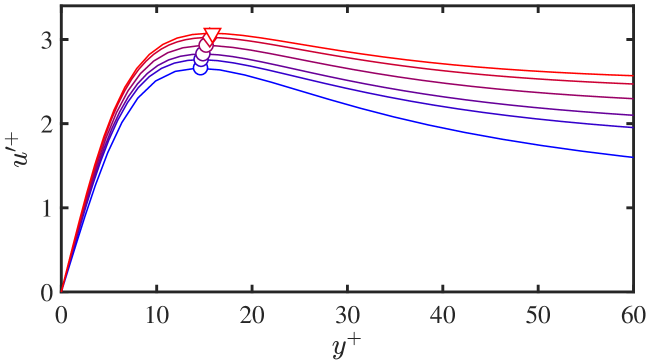
    (a)

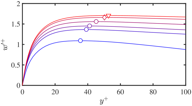
    (b)

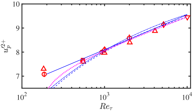
(c)

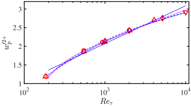
(d)

Figure 1: (a) Intensity of the streamwise velocity fluctuations near the wall. The symbols mark the position of the near-wall peak, as in table 1. Numerical channels [28, 23, 24]. The Reynolds number increases from blue to red in $Re_{\tau}=180-10^{4}$. (b) As in (a), for the spanwise velocity. (c) Peak intensity of the streamwise velocity fluctuations near the wall as a function of the Reynolds number. Symbols as in table 1, with standard deviations as vertical bars when available. (d) As in (c), for the spanwise velocity. Lines are different data fits:   , Logarithmic approximation [13], $u^{\prime 2+}_{p}=A_{L}+B_{L}\log(Re_{\tau})$;            , power defect law [8], $u^{\prime 2+}_{p}=A_{dP}+B_{dP}Re_{\tau}^{-1/4}$;                   , logarithmic defect law [10], $u^{\prime 2+}_{p}=A_{dL}+B_{dL}/\log(Re_{\tau})$;            , shifted logarithm, $u^{\prime 2+}_{p}=A_{S}+B_{S}\log(Re_{\tau}-150)$. Coefficients are collected in table 2.

Table 2: Coefficients for the line fits in Fig. 1.

	$A_{L},B_{L}$	$A_{dP},B_{dP}$	$A_{dL},B_{dL}$	$A_{S},B_{S}$
$u^{\prime 2}$	3.75, 0.63	11.5, -19.3	13.8, -40.0	4.17, 0.57
$w^{\prime 2}$	-0.97, 0.44	3.9, -10.0	5.18, -20.9	-0.18, 0.34

The fluctuation profiles and peak intensity of the two wall-parallel velocities are given in Fig. 1, which shows that they agree reasonably well with each other at similar Reynolds numbers. The growing trend of the profiles in Figs. 1(a,b) with the Reynolds number is clear, as is the trend of the peak position to slowly move away from the wall (for which there is some experimental evidence [29]).

The peak intensities are collected in Figs. 1(c,d), with line fits taken from the models discussed above with coefficients either taken from the original publications or fitted numerically to the data. They separate in two groups. The straight line is the basic logarithm already discussed above for the attached-eddy model [20, 5], which predicts an infinite intensity as $Re_{\tau}\to\infty$. The second group includes the dashed and chaindotted curves in each figure [8, 10], both of which assume a finite limit for the intensity, as in Eqs. (3) and (4). The defect formulations appear to represent the data better than the straight line of the logarithm, especially if we disregard the lowest Reynolds number, $Re_{\tau}\approx 180$, but the most striking observation is how similar to each other they are. Finally, the red dotted lines in the two figures are a shifted logarithm with a virtual origin for $Re_{\tau}$, which predicts an unbounded peak at large $Re_{\tau}$. It is not intended as a serious proposal, and I am not aware of any theoretical basis for it (although neither is it absurd to shift the Reynolds number by a transition threshold), but it shows that there are simple approximations that fit the available data as well as the defect laws, while predicting an infinite limiting value for the near-wall peak. It emphasizes that simple curve fitting cannot decide the issue.

It may be relevant at this point to estimate which would be the Reynolds number required to distinguish between the different fits in Figs. 1(c,d). An order of magnitude could be how far the logarithmic straight line has to be extended before it reaches the asymptotic value of any of the two defect laws. The details depend on the approximation and on the variable chosen, but it is in all cases of the order of $Re_{\tau}\approx 10^{5}$. This is at least 15–20 years in the future for numerical simulations, but it is worth remarking that experiments in pipes [29] up to $Re_{\tau}\approx 4\times 10^{4}$ have proved inconclusive for this purpose [10], and that data from the atmospheric surface layer at $Re_{\tau}=O(10^{6})$, although not strictly a channel, appear to follow the logarithmic trend reasonably well [11].

III The attached-eddy model

The key theoretical contribution to understanding the velocity fluctuations was made by Townsend [13], who noted that the usual argument that there is an overlap layer in which neither the viscous unit of length nor the flow thickness are relevant [4] should also apply to them. Although the resulting attached-eddy model has been reviewed often, we will recall it here to identify where the logarithmic prediction could go wrong.

The naive argument is that, if there is no scale for lengths, but $u_{\tau}$ is a scale for the velocities, the functional dependence of any variable with dimensions of velocity on a variable with dimensions of length should be logarithmic (see appendix A in Ref. 5). We could thus expect that $u^{\prime}/u_{\tau}\sim\log(y/h)$, which, when particularized at a fixed inner viscous limit, $y_{p}^{+}$, results in $u^{\prime}_{p}/u_{\tau}\sim\log Re_{\tau}$.

There is substantial experimental and numerical evidence for both approximate logarithmic behaviors [30], which, as mentioned above, extend to the fluctuations of the pressure and of the spanwise velocity[31] but, in the absence of a rigorous theory, it is always possible that higher Reynolds numbers than those currently available may lead to something different.

Moreover, there are logical flaws in the previous argument. Most obviously, an argument similar to the one used for $u^{\prime}$ applies to any power of the velocity, and some selection rule is needed to decide which power to use. In addition, the argument leading to the logarithm requires that the left-hand size (the velocity fluctuations) should be insensitive to an additive constant, because changing the length scale within the logarithm adds a constant to the overall expression. This is reasonable for the mean velocity in Eq. (1), for which a constant is a Galilean transformation, but less obvious for the fluctuations, which are defined with respect to a definite average. Finally, some reason should be found for why the logarithmic behavior applies to $u^{\prime}$ and $w^{\prime}$ but, as mentioned above, not to $v^{\prime}$, and a justification is required for why $u_{\tau}$ is the right scaling unit for the velocity fluctuations.

In general, it is unwise to use similarity arguments without a dynamical model, and Townsend [13] proposed that the logarithm is implemented by the superposition of a self-similar family of ‘attached’ Reynolds-stress-carrying eddies linking the wall to the interior of the flow. In the absence of a fixed length scale, their height is proportional to their wall-parallel size ($\lambda_{x}$ or $\lambda_{z}$), while their intensity is $O(u_{\tau})$ because each eddy family is responsible for carrying the tangential Reynolds stress $(-uv)$ at one distance from the wall. This is supported by observations: the solid contours in Figs. 2(a,b) are the premultiplied cospectra, $\Phi_{uv}^{+}(k_{x})$ and $\Phi_{uv}^{+}(k_{z})$ of the tangential Reynolds stress, respectively drawn as functions of $y$ and of the streamwise and spanwise wavelengths. The contours are normalized with the friction velocity, and the figures show that a stress $-uv\sim O(u_{\tau}^{2})$ is concentrated along a spectral ridge in which $\lambda_{x}\approx 25y$ and $\lambda_{z}\approx 5y$, and which extends from a minimum wavelength that scales in wall units to an outer one that scales with $h$. Since it can be shown that the streamwise and wall-normal velocities are well correlated, this extends the role of $u_{\tau}$ from a velocity scale for the overall intensity to one for individual spectral bands, but note that this argument applies to velocity fluctuations in the regions of the $\lambda-y$ plane where Reynolds stresses are substantial, but may not apply to ’sterile’ ones.

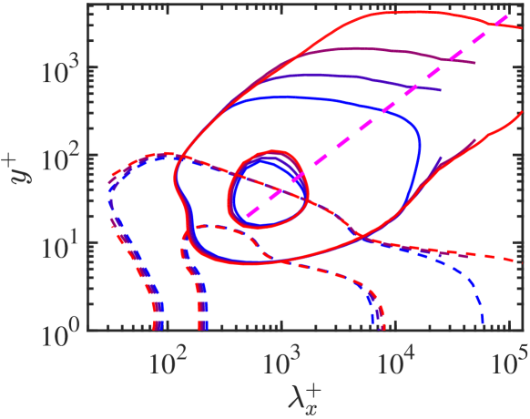
(a)

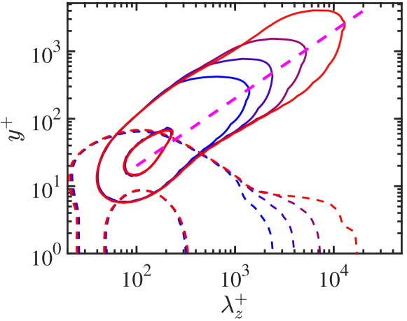
(b)

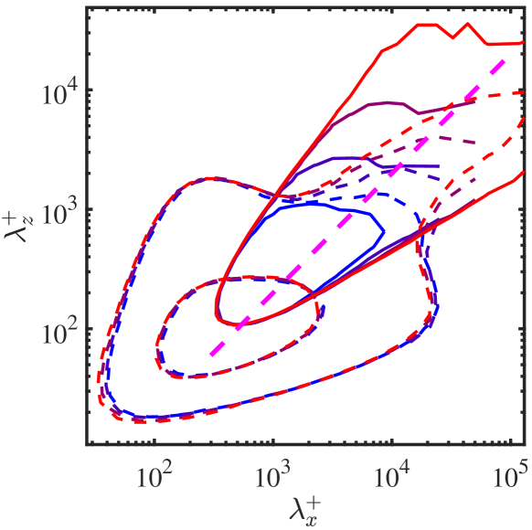
(c)

Figure 2: (a) Solid contours are premultiplied cospectra of the tangential Reynolds stress, $-\Phi_{uv}^{+}(\lambda_{x},y)=[0.2,\,0.8]$ times the common maximum of the four cospectra. Dashed ones are premultiplied spectra of the spanwise vorticity, $\Phi_{\omega_{z}\omega_{z}}^{+}(\lambda_{x},y)=[0.05,\,0.4]$ the common maximum. The dashed diagonal is $\lambda_{x}=25y$. (b) As in (a), but as functions of $\lambda_{z}$. The dashed diagonal is $\lambda_{z}=5y$. (c) Two-dimensional integrated spectra as functions of $(\lambda_{x},\lambda_{z})$: Solid contours are $-\int\Phi_{uv}^{+}{\,\rm{d}}y^{+}$ integrated over $y\in[0.005,\,0.5]\lambda_{x}$. Contours are $[0.2,\,0.8]$ the common maximum. Dashed ones are premultiplied spectra of the spanwise vorticity, $\int\Phi_{\omega_{z}\omega_{z}}^{+}{\,\rm{d}}y^{+}$, integrated over $y^{+}\in[0,\,20]$. Contours are $[0.05,\,0.4]$ the common maximum. The dashed diagonal is $\lambda_{x}=5\lambda_{z}$. Numerical channels [21, 23], with the Reynolds number increasing from blue to red: $Re_{\tau}=550,\,1000,\,2000,\,5200$.

Because there is no length scale, these bands are logarithmic (e.g. from $\lambda_{x}$ to $2\lambda_{x}$), and the number of eddy families found at a given distance $y$ from the wall is the number of logarithmic bands required to cover the range of lengths from $y$ to the flow thickness, $O(h)$, which increases logarithmically with $h/y$. If we further assume that the velocity fluctuations of the different bands are uncorrelated, their variances add, resulting in a logarithmic behavior with the Reynolds number for $u^{\prime 2+}(y)\sim\log(y/h)$ and for $u^{\prime 2+}(y_{p})$. Townsend [13] distinguishes between ‘inactive’ attached variables, such as $u^{\prime}$ and $w^{\prime}$, that are not sufficient to generate tangential Reynolds stress but are only damped by the wall in a thin viscous layer, and ‘active’ ones, like $v^{\prime}$, that contribute to the stress but are inhibited near the wall by impermeability. Only the former should have logarithmic profiles.

The difference between the two types of variables can be seen in Figs. 2(a,b), where the dashed lines are spectra of the spanwise vorticity. The flow at long wavelengths and at distances from the wall below the Reynolds-stress ridge can only be driven by the pressure footprint of the active eddies (see Fig. 12d in Ref. 5), and is therefore essentially irrotational. But potential flow cannot satisfy the no-slip condition at the wall, and a viscous rotational layer appears at long wavelengths below $y^{+}\lesssim 10$. Since $\omega_{z}\approx-\partial_{y}u$ in that region, this layer implies that there are non-trivial fluctuations of $u$ attached to the wall at those wavelengths. The solid contours in Fig. 2(c) are two-dimensional Reynolds-stress cospectra, integrated over the active band of wall distances corresponding to each wavelength, and the dashed ones are spectra of the spanwise vorticity integrated over the viscous near-wall layer. The figure strongly supports that the latter are the effect of the detached Reynolds stresses, although not necessarily at the same distance from the wall for all wavelengths.

Families of self-similar attached eddies, as well as the distinction between active and inactive motions, have been observed and characterised in some detail numerically [19, 32, 5] and experimentally [33, 34, 35, 17].

There are several debatable points in these arguments, most of which have been discussed in the literature and will not be repeated here, but some of them deserve closer attention. A well-known limitation of the attached-eddy model is that it does not include viscosity, whose effects are lumped into the rule that something happens below $y^{+}_{p}=15$. This has occasionally been suggested as responsible for scaling failures [10]. We have seen that what viscosity does is to generate the thin vortex layers in Fig. 2, but how they are maintained, their dimensions, and their effect are unclear, and we mentioned in the introduction that their stability is problematic if the fluctuations become too strong.

However, the overall conclusion from the previous discussion remains that the reason why velocity fluctuations do not scale well is that they contain a wide range of wavelengths, even when they are very close to the wall. This often-made point [14, 15, 36, 20] is clear from the spectra in Fig. 3 of the near-wall streamwise velocity at $y_{p}$. There is a universal ‘core’ at $\lambda_{x}^{+}\times\lambda_{z}^{+}\approx 1000\times 100$, which does not reach above $y^{+}\approx 100$ (Fig. 2) and collapses well across $Re_{\tau}$. That its dimensions scale in wall units shows that it is controlled by viscosity [37, 38, 39], but it is accompanied by larger-scale spectral tails that extend to $\lambda\sim O(h)$, and are responsible for the extra energy of the overall fluctuations. A corollary is that the dynamics of these tails, which does not have to be the same as for the viscous core, has to be studied if the overall peak is to be understood.

This wide range of scales is a problem for asymptotic models that seek to expand the flow in terms of an outer ‘regular’ turbulence and a small-scale object near the wall, which does not exist as such in real flows. In fact, given that the total peak energy includes contributions from a wide range of wavelengths, it is unclear whether it makes sense to speak of a single velocity and length scale for it.

(a)

Figure 3: Premultiplied energy spectrum of the streamwise velocity $\Phi_{uu}^{+}$ at $y^{+}=15$, versus the wall-parallel wavelengths. Numerical channels [21, 23], with the Reynolds number increasing from blue to red: $Re_{\tau}=550,\,1000,\,2000,\,5200$. Contours are $[0.15,\,0.4,\,0.8]$ times the common maximum of the four spectra. The dashed diagonal is $\lambda_{x}=12\lambda_{z}$, and symbols are $\lambda_{z}=h$. The translucent patch is used in Fig. 5.

IV The large scales

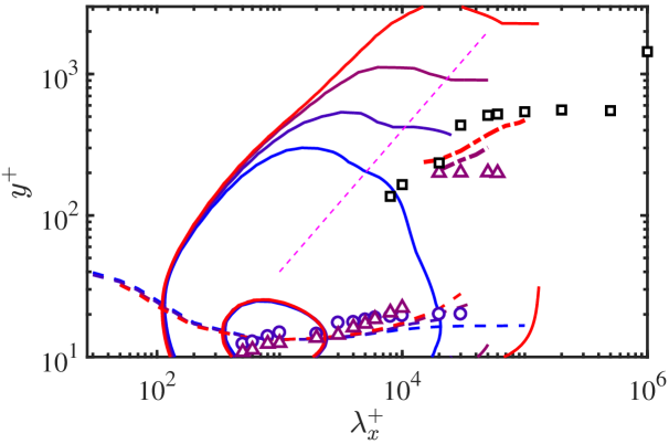
(a)

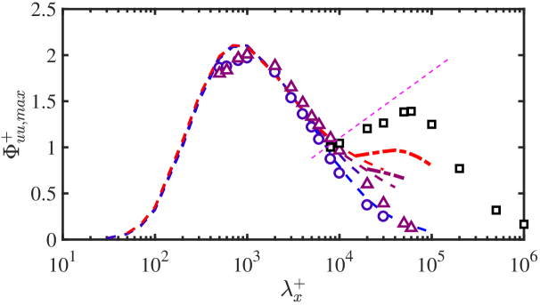
(b)

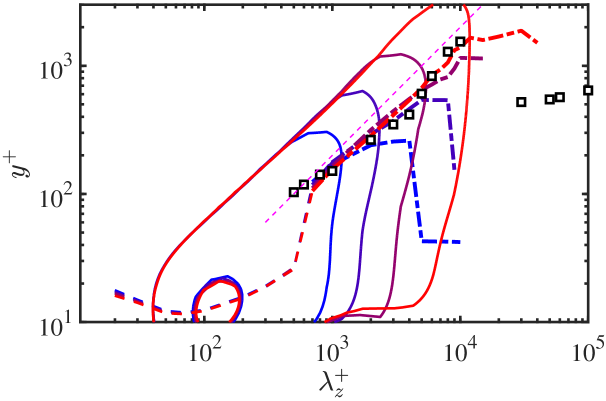
(c)

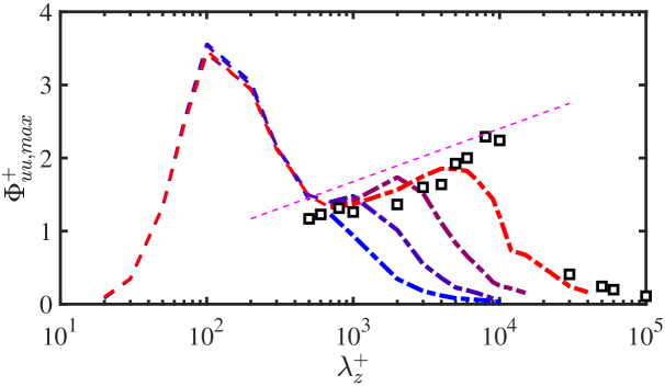
(d)

Figure 4: (a,c) Contours are the premultiplied spectrum of the streamwise velocity. The contours are $[0.2,\,0.8]$ times the overall maximum of all the $\Phi_{uu}^{+}$. Dashed and chaindotted lines are the location of the inner and outer maxima of $\Phi_{uu}$ at each wavelength. Numerical channels [21, 23], with the Reynolds number increasing from blue to red: $Re_{\tau}=550,\,1000,\,2000,\,5200$. Symbols are boundary layers in Ref. 40: $\circ$, $Re_{\tau}=1014$; $\vartriangle$, 1844; and $\square$, $Re_{\tau}=14000$ from Ref. 17. (b,d) Maximum of $\Phi_{uu}^{+}$ versus wavelength, with the same lines and symbols. (a,b) Against $\lambda_{x}$. (c,d) Against $\lambda_{z}$. The dashed magenta line in (a) and (c) are $\lambda_{x}^{+}=25y^{+}$ and $\lambda_{z}^{+}=5y^{+}$, respectively. The ones in (b) and (d) are $\Phi_{uu,max}^{+}=0.315\log(\lambda_{x}^{+})-1.8$ and $\Phi_{uu,max}^{+}=0.315\log(\lambda_{z}^{+})-0.5$.

Figures 4(a,c) are similar to the cospectra in Figs. 2(a,b), but drawn for the streamwise velocity component. To facilitate comparison, the dashed diagonals in the two figures are the same, and show that the vertical extent of the kinetic energy and of the Reynolds stress are similar, but it is clear from Fig. 4 that the streamwise velocity spectrum extends to the wall, while the cospectrum stays away from it. Figure 4 includes as dashed lines and symbols the wall-normal location of the maximum of $\Phi_{uu}$ at each wavelength.

We saw when discussing Fig. 1 that the energy peak drifts slowly away from the wall with the Reynolds number, and Figs. 4(a,c) show a clearer dependence on the wavelengths. The symbols are from experimental boundary layers [40, 17] and, although sparser near the wall, are compatible with the numerics. The inner maximum at the shorter wavelengths marks the edge of the viscous layer, and is substituted beyond $\lambda_{x}^{+}\approx 10^{4}$ by an outer maximum located at $y\approx\lambda_{z}/5$ (Fig. 4c). The amplitude of these maxima is shown in Figs. 4(b,d). It collapses well with $Re_{\tau}$ in the viscosity-dominated region, $\lambda_{x}^{+}\lesssim 10^{4}$ or $\lambda_{z}^{+}\lesssim 10^{3}$, but not at the larger wavelengths associated with the outer maximum. Their growth with $\lambda$ can be interpreted as a wavelength-by-wavelength counterpart to the logarithmic growth of $u^{\prime 2}_{p}$ with $Re_{\tau}$, represented here by the range of wavelengths over which the one-dimensional spectrum is summed. We have added to Figs. 4(b,d) logarithmic approximations to this growth, using half the slope in Fig. 1 for $u^{\prime 2}_{p}$, on the assumption that half of the peak growth is due to the wider range of $\lambda_{x}$ and the other half to the wider range of $\lambda_{z}$. These logarithms match the data relatively well, but they should only be considered as aids to the eye, subject to the same caveats as in Fig. 1(a,b).

Fortunately, more can be said about the larger flow scales. The outer maximum of the longest structures in Fig. 4(a) represents layers of dimensions $(\lambda_{x}\times y\times\lambda_{z})^{+}=O(20000\times 500\times 4000)$, which are thin both with respect to the channel height $(Re_{\tau}=5200)$ and to their own length. They are also deep enough to be fully turbulent. Internal turbulent layers are common when wall-bounded flows cross boundaries between different types of wall or are otherwise perturbed, and have been extensively studied in meteorology [41, 42] and for heterogeneous surfaces [43]. Using a rough approximation [42], there is an internal equilibrium layer (EL) whose thickness after time $\Delta t$ grows to $\delta_{EL}\approx u_{\tau}\Delta t/4$, and satisfies the universal velocity profile corresponding to the friction velocity that develops after the perturbation. Since the lifetime of the stress-carrying structures is [44] $\Delta t\approx\Delta y/u_{\tau}\approx\lambda_{z}/u_{\tau}$, the thickness of the EL generated by perturbations of width $\lambda_{z}$ is $\delta_{EL}\approx\lambda_{z}/4$, which is approximately the location of the outer maximum in Fig. 4(c) .

The model is that large-scale fluctuations with wavelengths of the order of $\lambda^{+}_{x}\approx 5\lambda^{+}_{z}\gtrsim 10^{4}$ (Fig. 2c) are equilibrium turbulent boundary layers satisfying the universal profile $U=u_{\tau}F(y^{+})$ with a perturbed friction velocity, and that, if they are viewed as perturbations to the overall mean velocity, they can be modeled as weak perturbations of $u_{\tau}\to u_{\tau}+\delta u_{\tau}$. Upon linearization,

$$(\delta U)=(\delta u_{\tau})(F+y^{+}{\rm{d}}F/{\rm{d}}y^{+})=(\delta u_{\tau})G(y^{+}),$$ (5)

which links the rms intensity of the velocity fluctuations to the rms perturbation of the friction velocity, $(\delta u_{\tau})^{\prime}=u_{*}$. In the viscous layer, $F=y^{+}$, and

$$(\delta U)^{\prime}/u_{*}=2y^{+}.$$ (6)

This is essentially the modulation described in [45], which was shown in [46] to reduce in the buffer layer to a modulation of $u_{\tau}$. We extend it here to the logarithmic layer, where $F$ satisfies (1), and

$$(\delta U)^{\prime}/u_{*}=\kappa^{-1}\left(1+A\kappa+\log y^{+}\right).$$ (7)

These equations are tested in figure 5(a) for spectral densities within the patch of large-scale tails in Fig. 3. The perturbation intensity, $u_{*}$, of the friction velocity has been adjusted for each wavelength to fit Eq. (5) to the spectral profile from the wall to its maximum, but the definition of $F$ has not been modified. The symbols in Fig. 5(a) are $G(y^{+})$ in Eq. (5), computed from the mean velocity $F(y^{+})$ of a turbulent channel, and the agreement is excellent. Figure 5(b) shows that the required $u_{*}$ scales with $\lambda_{x}/h$ rather than in wall units. Note that the lowest $Re_{\tau}=550$ is not in the figure because it never develops an outer peak. The rms of the fluctuations of $u_{\tau}$ tend to some non-zero value when $\lambda_{x}\to 0$, so that the fluctuation velocity profile can be approximated as

$$u^{\prime 2+}(y^{+})=u^{\prime 2+}_{s}(y^{+})+G^{2+}(y^{+})\int_{\lambda_{1}/h}^{\lambda_{2}/h}u_{*}^{2+}(\lambda/h){\,\rm{d}}\log\lambda,$$ (8)

where $G(y^{+})$ is defined in Eq. (5), $\lambda_{1}=\max(\lambda_{in},5y)$, and $u^{\prime 2+}_{s}$ is the contribution of scales whose $\lambda_{x}$ is shorter than the wavelength, $\lambda_{in}$, at which the viscous sublayer becomes unstable and fluctuations have to be modeled as turbulent profiles. It is important to note that the lower limit of this integral scales in wall units ($\lambda_{in}^{+}\approx 10^{4}$ in Fig. 4), while the upper one either extends to infinity, or scales in outer units ($\lambda_{2}=25h$ in our case to accommodate the length of our computational box). Assuming that the small-scale contribution to Eq. (8) is independent of $Re_{\tau}$, and that the integral of $u_{*}^{2}$ stays bounded at $\lambda\to\infty$, the dominant contribution to Eq. (8) at high $Re_{\tau}$ comes from the lower limit of the integral,

$$u^{\prime 2+}(y^{+})\approx u^{\prime 2+}_{s}(y^{+})+G^{2+}(y^{+})u_{*}^{2+}(0)\log(Re_{\tau}/\lambda_{in}^{+}).$$ (9)

It is important to realize that $U+\delta U$ in Eq. (5) is the mean profile of a perturbed boundary layer. These faster- or slower-than-average local equilibrium layers also have small-scale perturbations that are modulated by the outer Reynolds-stress structures, but those are second-order effects, negligible with respect to the mean profile. The maximum fluctuation intensity at the inner energy peak is $u^{\prime 2}_{p}\approx 9$, while the mean velocity at that point is $U^{2+}(y_{p})\approx 100$. The fluctuation profiles are only relevant if the mean profile can be considered fixed, but any perturbation of the latter overwhelms the modulation of the small scales.

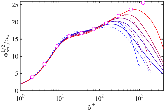
(a)

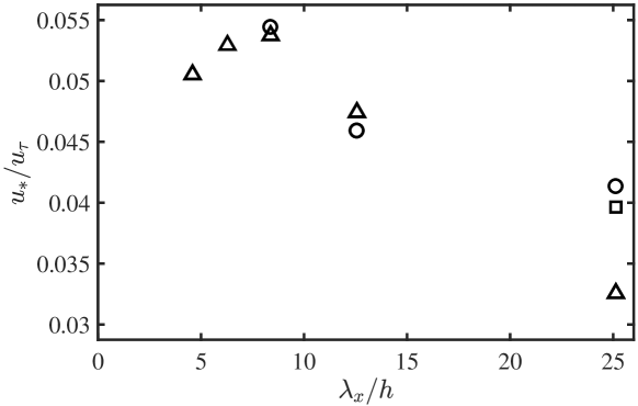
(b)

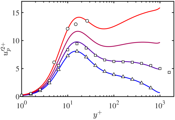
(c)

Figure 5: (a) Spectral density of the streamwise velocity for various wavelengths, from $\lambda_{x}^{+}=2\times 10^{4}$ to $\lambda_{x}=25h$, from blue to red, integrated in $\lambda_{z}$ over the diagonal band in Fig 3, defined as $\lambda_{z}\in\lambda_{x}/[5,\,30]$. The symbols are $G$ in Eq. (5), computed from the mean velocity profile in [23]. (b) Friction velocity perturbation intensities obtained from (a). Channels [23]: (                    and $\square$) $Re_{\tau}=1000$; (             and $\circ$) $Re_{\tau}=2000$; (    and $\vartriangle$) $Re_{\tau}=5200$. (c) Lines are fluctuation profiles estimated from Eq. (8). From bottom to top: $Re_{\tau}=1000,\,10^{4},\,10^{5}$ and $2\times 10^{6}$. Symbols are channel simulations [23, 24] and the atmospheric surface layer [12] at those Reynolds numbers.

Eq. (9) is also a logarithm that diverges as $Re_{\tau}\to\infty$, but its most interesting aspect is that the form of the large-scale correction is not a peak near the wall, but something similar to the mean velocity profile of a regular boundary layer, so that the fluctuation peak will be absorbed into something closer to a plateau at high $Re_{\tau}$. Although estimating this behavior necessarily implies extrapolation from lower Reynolds numbers, Fig. 5(c) plots Eq. (8) for several large $Re_{\tau}$. The lowest curve in the figure, $Re_{\tau}=1000$ is used to estimate the viscous contribution $u^{\prime}_{s}$, and is therefore automatically fitted. But the corrections for the rest of the curves are computed by estimating the integral in Eq. (8), using a lineal least-square approximation to $u_{*}$ in Fig. 5(b). The agreement with our highest Reynolds number, $Re_{\tau}=10^{4}$ is excellent, and it is intriguing that the uppermost curve in the figure, intended to approximate data from the atmospheric surface layer[12], also appears to fit well. The fluctuation profile in this case is already very different from that at lower Reynolds numbers, including a second outer maximum of $u^{\prime}$, and requires experimental confirmation. Although the implied $Re_{\tau}=O(10^{6}-10^{7})$ are well in the future for laboratory or numerical flows, they are not out of range for geophysical ones [11, 12].

Figure 6: Premultiplied energy spectrum of the spanwise velocity, $\Phi_{ww}^{+}$ at $y^{+}=50$, versus the wall-parallel wavelengths. Numerical channels [21, 23] with the Reynolds number increasing from blue to red: $Re_{\tau}=550,\,1000,\,2000,\,5200$. Contours are $[0.15,\,0.4,\,0.8]$ of the common maximum of the four spectra. The dashed diagonal is $\lambda_{x}=6\lambda_{z}$ and symbols are $\lambda_{z}=h$. The translucent patch is used in Fig. 7(c,d).

V The spanwise velocity

Up to now we have mostly dealt with the streamwise velocity fluctuations, but it is clear from Fig. 1 that the spanwise velocity also has a potentially infinite limit. Figure 6 displays the two-dimensional spectrum of $w^{\prime}$, and shows that the reason is also the effect of large structures whose size scales with $h$ rather than in wall units, although they are wide rather than long, as required by continuity [47].

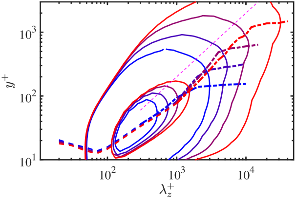
(a)

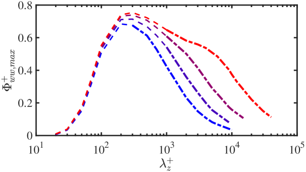
(b)

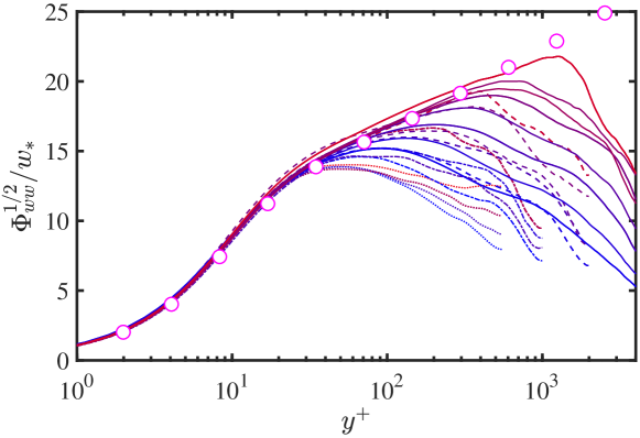
(c)

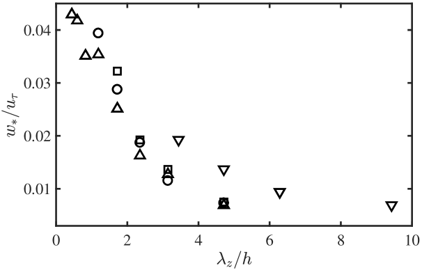
(d)

Figure 7: (a) Premultiplied spectrum of the spanwise velocity versus $\lambda_{z}$. The contours are $[0.2,\,0.8]$ times the overall maximum of all the $\Phi_{ww}^{+}$. Dashed and chaindotted lines are the location of the inner and outer maxima of $\Phi_{ww}$ at each wavelength. Numerical channels [21, 23], with the Reynolds number increasing from blue to red: $Re_{\tau}=550,\,1000,\,2000,\,5200$. The dashed magenta line is $\lambda_{z}^{+}=5y^{+}$. (b) Maximum of $\Phi_{ww}$ versus wavelength, with the same lines as in (a). (c) Spectral density of the spanwise velocity for various wavelengths from $\lambda_{z}^{+}=2\times 10^{3}$ to $\lambda_{z}=10h$, from blue to red, integrated in $\lambda_{x}$ over the diagonal band in Fig 6, defined as $\lambda_{x}\in[2,\,20]\lambda_{z}$. The symbols are the perturbation equilibrium Eq. (10), computed from the mean velocity profile in [23]. (d) Friction velocity perturbation intensities obtained from (c). (            and $\triangledown$) Channel [21], $Re_{\tau}=550$; the rest are channels [23]: (                    and $\square$) $Re_{\tau}=1000$; (             and $\circ$) $Re_{\tau}=2000$; (    and $\vartriangle$) $Re_{\tau}=5200$.

The perturbation expansion is also slightly different from the streamwise component. The first term in the expression for $G$ in Eq. (5) comes from the boundary layer created by the perturbation of $u_{\tau}$, which in this case has to be oriented spanwise. The second term is the deformation of the existing boundary layer by the change in length scale due to the new $u_{\tau}$, and is missing from $\delta W$, for which no preexisting spanwise flow exists. The fluctuation equation becomes,

$$(\delta W)^{\prime}=(\delta w_{\tau})^{\prime}F(y^{+})=w_{*}F(y^{+}),$$ (10)

where $F(y)$ is, as before, the mean velocity profile of a regular channel, and the symbols $w_{\tau}$ and $w_{*}$ have been introduced to represent the friction velocity of the spanwise perturbation flow.

Figure 7 summarizes for the spanwise velocity the same information as Figs. 4 and 5 do for $u$. As in the previous case, the relevant result is that the transition from the inner to the outer peak scales in wall units, at approximately the same wavelength as for the streamwise velocity, $\lambda_{z}^{+}\approx 1000$, (Fig. 7a,b). Conversely, the perturbation friction velocity required to fit the profiles in Fig. 7(c) to Eq. (10) scales well in outer units (Fig. 7d), so that its total energy also diverges logarithmically. Notice that the fit of Eq. (10) to the data in Fig. 7(c) is as good as that in Fig. 5, even if the two predicted profiles are fairly different.

There are some differences between the two velocity components. The $\Phi_{ww}$ spectra in Fig. 7(a) are consistently wider and taller than $\Phi_{uu}$ in Fig. 4(c). The outer peak of $\Phi_{ww}$ follows $\lambda_{z}\approx 10y$ instead of $\lambda_{z}\approx 5y$, and the distinction between inner and outer intensities in Fig. 7(b) is much less clear than in Fig. 4(d). While the inner and outer peaks of $\Phi_{uu}$ are often two distinct maxima separated in $y$, those of $\Phi_{ww}$ are a single maximum whose location depends on $\lambda$. There are essentially no bimodal intensity profiles in $\Phi_{ww}$.

The distribution of perturbation friction velocities is also different in the two cases. Although both scale in outer units, the distribution in Fig. 5(b) is fairly regular, with what appears to be a definite limit at $\lambda_{x}=0$, but Fig. 7(d) may have a more singular interpretation.

VI Discussion and conclusions

In summary, we have seen that, as most things in turbulence, the near-wall region is a multi-scale flow involving widely different ranges of length and width. In consequence, the near-wall peak of the stream- and spanwise velocity fluctuation intensities cannot be modeled as an elementary object. There is a viscosity-dominated core $(\lambda^{+}_{x}\times\lambda^{+}_{z}\approx 1000\times 100$) which embodies the classical turbulence cycle and scales well across Reynolds numbers, and a large-scale component that behaves very differently. The high-Reynolds-number limit of the energy depends on those large scales, which we have explored using spectra. It turns out that they behave near the wall as internal equilibrium boundary layers, excited by the pressure footprint of the outer large eddies. Their mean velocity profiles appear as fluctuations with respect to the overall average flow, and become part of what is known at low Reynolds numbers as the near-wall peak.

The intensity of these large-scale fluctuations is predicted to increase logarithmically with $Re_{\tau}$, but not to remain concentrated near the wall. At extremely large Reynolds numbers, they should spread to a fraction of the channel thickness, of the order $O(h/5)$. We have shown that their profile can be extracted at laboratory Reynolds numbers from the vertical structure of the spectrum at particular wavelengths. When extrapolated t geophysical Reynolds numbers they result in a fairly different fluctuation profile including, interestingly, a second maximum away from the wall.

In fact, the natural consequence of a model in which most of the near-wall kinetic energy at high Reynolds number is driven by interactions with the outer flow is that even this near-wall region, and any part the boundary layer whose distance from the wall is fixed in wall units, should be considered as directly driven by the outer flow. Under those circumstances, and even if the velocity scale for the active turbulence motions responsible for the Reynolds stresses continues to be the friction velocity, a more natural unit for the inactive motions may be some measure of the driving velocity ($U_{\infty}$, $U_{bulk}$ or some other velocity combination such as the mixed scaling in [6]). It is interesting to note that, if we recall from Eq. (1) that $U_{\infty}\sim\log Re_{\tau}$, even a logarithmic growth of $u^{\prime 2+}_{p}$ implies that $u^{\prime}_{p}/U_{\infty}\sim\log^{-1/2}Re_{\tau}\to 0$ as $Re_{\tau}\to\infty$. The nature of the singularity is not that $u^{\prime}_{p}$ tends to infinity, but that $u_{\tau}\to 0$ faster than $u^{\prime}_{p}$.