Polarization effects in the elastic $e\vec{p}\to\vec{e}p$ and $\vec{e}\vec{p}\to ep$
processes in the case of parallel spins

Abstract

In the one-photon exchange approximation, we analyze polarization effects in the elastic $\vec{e}\vec{p}\to ep$ and $e\vec{p}\to\vec{e}p$ processes in the case when the spin quantization axes of a target proton at rest and an incident or scattered electron are parallel. To do this, in the kinematics of the SANE Collaboration experiment [A. Liyanage et al., Phys. Rev. C 101, 035206 (2020)] using the J. Kelly [Phys. Rev. C 70, 068202 (2004)] and [I. Qattan et al. Phys. Rev. C 91, 065203 (2015)] parametrizations for the Sachs form factor ratio $R\equiv\mu_{p}G_{E}/G_{M}$, a numerical analysis was carried out of the dependence of the longitudinal polarization degree transferred to the scattered electron in the $e\vec{p}\to\vec{e}p$ process and double spin asymmetry in the $\vec{e}\vec{p}\to ep$ process on the square of the momentum transferred to the proton as well as on the scattering angle of the electron. It is established that the difference in the longitudinal polarization degree of the scattered electron in the $e\vec{p}\to\vec{e}p$ process in the case of conservation and violation of the scaling of the Sachs form factors can reach 70 %. This fact can be used to set up polarization experiments of a new type to measure the ratio $R$. For double spin asymmetry in the $\vec{e}\vec{p}\to ep$ process, the corresponding difference of the $R$ ratio does not exceed 2.32 %. This fact means that it is not sensitive to the effects of the Sachs form factor scaling violation and could be used as a test for the $R\approx 1$ equality.

I Introduction

Experiments on the study of electric $G_{E}$ and magnetic $G_{M}$ proton form factors, the so-called Sachs form factors (SFFs), have been performed since the mid-1950s in the elastic process of electron-proton scattering Hofstadter1958 . In the case of unpolarized electrons and protons, all experimental data on the behavior of the SFFs were obtained with the help of the Rosenbluth technique (RT) based on the Rosenbluth formula for the differential cross section for the $ep\to ep$ process in the rest frame of the initial proton Rosen ; that is,

$$\frac{d\sigma}{d\Omega_{e}}=\frac{\alpha^{2}E_{2}\cos^{2}(\theta_{e}/2)}{4E_{1}^{3}\sin^{4}(\theta_{e}/2)}\frac{1}{1+\tau_{p}}\left(G_{E}^{2}+\frac{\tau_{p}}{\varepsilon}G_{M}^{2}\right).$$ (1)

Here $\tau_{p}=Q^{2}/4m^{2},Q^{2}=4E_{1}E_{2}\sin^{2}(\theta_{e}/2)$ is the square of the 4-momentum transferred to the proton; $m$ is the mass of the proton; $E_{1}$, $E_{2}$ are the energies of the initial and final electrons, $\theta_{e}$ is the electron scattering angle; $\varepsilon=[1+2(1+\tau_{p})\tan^{2}(\theta_{e}/2)]^{-1}$ is the degree of linear (transverse) polarization of the virtual photon Dombey ; Rekalo74 ; AR ; GL97 ; $\alpha=1/137$ is the fine structure constant. Expression (1) was obtained in the one-photon exchange (OPE) approximation and the electron mass was set to zero.

With the help of RT, the dipole dependence of the SFFs on the momentum transferred to the proton square $Q^{2}$ in the region $Q^{2}\leq 6$ $\mbox{GeV}^{2}$ was established ETG15 ; Punjabi2015 . As it turned out, $G_{E}$ and $G_{M}$ are related by the scaling ratio $G_{M}\approx\mu_{p}G_{E}$ ($\mu_{p}=2.79$ is the magnetic moment of the proton), and for their ratio $R\equiv\mu_{p}G_{E}/G_{M}$, the approximate equality $R\approx 1$ is valid.

Akhiezer and Rekalo Rekalo74 proposed a method for measuring the $R$ ratio based on the phenomenon of polarization transfer from the initial electron to the final proton in the $\vec{e}p\to e\vec{p}$ process (later this method was generalized in Ref. Miller2015 ). Precision JLab experiments Jones00 ; Gay01 ; Gay02 , using this method, found a fairly rapid decrease in the ratio of $R$ with an increase in $Q^{2}$, which indicates the violation of the dipole dependence (scaling) of the SFFs. In the range $0.4~{}\mbox{GeV}^{2}\leqslant Q^{2}\leqslant 5.6~{}\mbox{GeV}^{2}$, as it turned out, this decrease is linear. Next, more accurate measurements of the ratio $R$ carried out in Pun05 ; Puckett10 ; Puckett12 ; Puckett17 ; Qattan2005 in a wide area in $Q^{2}$ up to $8.5~{}\mbox{GeV}^{2}$ using both the Akhiezer – Rekalo (AR) method Rekalo74 and the RT Qattan2005 , only confirmed the discrepancy of the results.

In the SANE Collaboration experiment Liyanage2020 , the values of $R$ were obtained by the third method Donnelly1986 by extracting them from the results of measurements of double spin asymmetry in the $\vec{e}\vec{p}\to ep$ process in the case, when the electron beam and the proton target are partially polarized. The degree of polarization of the proton target was $P_{t}=(70\pm 5)$%. The experiment was performed at two electron beam energies $E_{1}$, 4.725 GeV and 5.895 GeV, and two $Q^{2}$ values, 2.06 GeV² and 5.66 GeV². The extracted values of $R$ in Liyanage2020 are consistent with the results in Refs. Jones00 ; Gay01 ; Gay02 ; Pun05 ; Puckett10 ; Puckett12 ; Puckett17 .

The presence of a highly polarized proton target motivates the study of polarization effects (including double spin correlations) in the processes such as $e\vec{p}\to e\vec{p}$, $e\vec{p}\to\vec{e}p$, $\vec{e}\vec{p}\to ep$.

In JETPL2008 ; JETPL18 ; JETPL19 ; JETPL2021 ; PEPAN2022 ; JETPL2022 , in the OPE approximation, polarization effects in the elastic $e\vec{p}\to e\vec{p}$ process were investigated in the case when the spins of the initial and of the detected recoil proton are parallel, i.e., when an proton is scattered in the direction of the spin quantization axis of the rest proton target. To do this, in the kinematics of the SANE Collaboration experiment Liyanage2020 on measuring double-spin asymmetry in the $\vec{e}\vec{p}\to ep$ process, using the Kelly Kelly2004 and Qattan Qattan2015 parametrizations for the $R$ ratio, a numerical analysis was carried out of the dependence of the longitudinal polarization degree of the scattered proton on the square of the momentum transferred to the proton as well as on the scattering angle of the electron and proton. In this case, a noticeable sensitivity of the transferred to the proton polarization to the type of dependence of the ratio $R$ on $Q^{2}$ was established, and it was also shown that the violation of the scaling of the SFFs leads to a significant increase in the magnitude of the polarization transfer to the proton, as compared to the case of the dipole dependence. Thus, in JETPL2008 ; JETPL18 ; JETPL19 ; JETPL2021 ; PEPAN2022 ; JETPL2022 , the 4th method for measuring the ratio of $R$ was proposed, based on the transfer of polarization from the initial proton to the final one in the $e\vec{p}\to e\vec{p}$ process in the case when their spins are parallel. This line of research was started in JETPL2008 . This method also works in the two-photon exchange (TPE) approximation and allows us to measure the squares of the modules of generalized SFFs JETPL19 .

Note that Akhiezer and Rekalo (see AR , pp. 211–215) also performed a general calculation of the $e\vec{p}\to e\vec{p}$ cross section in the Breit system for partially polarized initial and final protons. However, they analyzed this cross section in AR by analogy with Rekalo74 and overlooked a more interesting case, which was discussed in JETPL2008 ; JETPL18 ; JETPL19 ; JETPL2021 ; PEPAN2022 ; JETPL2022 .

In our recent short paper PRD2023 , the 5th method of measuring the ratio $R$ was proposed, based on the transfer of polarization from the initial proton to the final electron in the elastic $e\vec{p}\to\vec{e}p$ process in the case when the spins quantization axes of the resting proton target and the scattered electron are parallel, i.e., when the electron is scattered in the direction of the spin quantization axes of the resting proton target.

The aim of this article is to give a more detailed view of the results of the work PRD2023 , as well as to investigate the double spin asymmetry in the $\vec{e}\vec{p}\to ep$ process in the case of parallel spins of the initial electron and proton. To do this, in the kinematics of the SANE Collaboration experiment Liyanage2020 using the Kelly Kelly2004 and Qattan Qattan2015 parametrizations for the SFF ratio $R$, a numerical analysis was carried out of the dependence of the longitudinal polarization degree transferred to the scattered electron in the $e\vec{p}\to\vec{e}p$ process and the double spin asymmetry in the $\vec{e}\vec{p}\to ep$ process on the square of the momentum transferred to the proton, as well as on the scattering angle of the electron.

II Helicity and diagonal spin bases

The spin 4-vector $s=(s_{0},\mbox{\boldmath$s$})$ of the fermion with 4-momentum $p$ ($p^{2}=m^{2})$ satisfying the conditions of orthogonality and normalization is given by

$$s=(s_{0},\mbox{\boldmath$s$}),\;s_{0}=\frac{\mbox{\boldmath$c$}\,\mbox{\boldmath$p$}}{m},\;\mbox{\boldmath$s$}=\mbox{\boldmath$c$}+\frac{\,(\mbox{\boldmath$c$}\,\mbox{\boldmath$p$})\,\mbox{\boldmath$p$}}{m(p_{0}+m)\,},$$ (2)

where $c$ is the spin quantization axis ($\mbox{\boldmath$c$}^{2}=1$).

Expressions (2) allow us to determine the spin 4-vector $s=(s_{0},\mbox{\boldmath$s$})$ by a given 4-momentum $p=(p_{0},\mbox{\boldmath$p$})$ and 3-vector $c$. On the contrary, if the 4-vector $s$ is known, then the spin quantization axis $c$ is given by

$$\mbox{\boldmath$c$}=\mbox{\boldmath$s$}-\frac{s_{0}}{p_{0}+m}\,\mbox{\boldmath$p$},$$ (3)

i.e. the vectors $c$ and $s$ at a given $p$ uniquely define each other.

For calculation of polarization effects in high-energy physics process one usually utilize helicity basis introduced by Jacob and Wick Jacob , in which the spin quantization axis $c$ is directed along the momentum of the particle

$$\mbox{\boldmath$c$}=\mbox{\boldmath$n$}=\mbox{\boldmath$p$}/|\mbox{\boldmath$p$}|,$$ (4)

while the spin 4-vector $s$ (2) reads

$$s=(s_{0},\mbox{\boldmath$s$})=(|\mbox{\boldmath$v$}|,v_{0}\,\mbox{\boldmath$n$}),$$ (5)

where $v_{0}$ and $v$ are the time and space components of the 4-velocity vector $v=p/m$ ($v^{2}=1$).

The popularity of the helicity basis is primarily due to the simplicity of the physical interpretation of the helicity definition (projection of the spin in the direction of the particle momentum), and its emphasis on the center of mass system. At the same time, studying of helicities of moving particles is analogous to the study of the spins of particles at rest GL ; FIF70 . However, there are several important factors which prevent helicity from playing the dominant role in describing the spin projection of particles. One is that helicity is not a particle characteristic that is invariant under the Lorentz transformation GL ; FIF70 ; AB ; BLP . In interpreting the dynamics of spin interaction, the amplitudes of scattering processes with and without changing the sign of the particle helicity are often referred to as amplitudes with and without a spin flip. However, since the particle momentum is changed by the interaction, it is clear that such a classification is very arbitrary. Both types of amplitudes actually describe a process with a change in the particle spin state.

In general, for a system of two particles with different 4-momenta $q_{1}=(q_{10},\mbox{\boldmath$q_{1}$})$ (before interaction) and $q_{2}=(q_{20},\mbox{\boldmath$q_{2}$})$ (after interaction) the possibility of quantization of spins in one common direction, including the case when particles have different masses, is determined by the three-dimensional vector given by FIF70

$$\mbox{\boldmath$a$}=\mbox{\boldmath$q$}_{2}/q_{20}-\mbox{\boldmath$q$}_{1}/q_{10}.$$ (6)

Since the common spin quantization axis (6) defines the spin basis other than the helicity one (4) and is the difference of two three-dimensional vectors, the geometric image of which is the diagonal of a parallelogram, it is natural to call it the diagonal spin basis (DSB). For the first time, in a four-dimensional covariant form, the DSB was constructed in the work Sik84 in the process

$$e(p_{1})+p\,(q_{1},s_{p_{1}})\to e(p_{2})+p\,(q_{2},s_{p_{2}}).$$ (7)

In it, the spin 4-vectors of the initial and final protons $s_{p_{1}}$ and $s_{p_{2}}$ are expressed in terms of their 4-momenta $q_{1}$ and $q_{2}$ ($q_{1}^{2}=q_{2}^{2}=m^{2}$) Sik84 :

$$s_{p_{1}}=\frac{m^{2}q_{2}-(q_{1}q_{2})\,q_{1}}{m\sqrt{(q_{1}q_{2})^{2}-m^{4}}}\,,$$ (8)

$$s_{p_{2}}=\frac{(q_{1}q_{2})\,q_{2}-m^{2}q_{1}}{m\sqrt{(q_{1}q_{2})^{2}-m^{4}}}\,.$$ (9)

In the laboratory frame (LF), where the initial proton rests, $q_{1}=(m,\mbox{\boldmath$0$})$, the spin 4-vectors (8) and (9) read

$$s_{p_{1}}=(0,\mbox{\boldmath$n$}_{2})\,,\;s_{p_{2}}=(|\mbox{\boldmath$v$}_{2}|,v_{20}\,\mbox{\boldmath$n_{2}$}),$$ (10)

where $\mbox{\boldmath$n$}_{2}=\mbox{\boldmath$q_{2}$}/|\mbox{\boldmath$q$}_{2}|$, $v_{2}=(v_{20},\mbox{\boldmath$v$}_{2})=q_{2}/m$ is the velocity vector of the final proton, $v_{2}^{2}=1$.

Using the explicit form of the spin 4-vectors (10) and formulas (3) or (6), it is easy to verify that the spin quantization axes of the initial and final proton in the LF coincide with the direction of the final proton momentum

$$\mbox{\boldmath$c$}=\mbox{\boldmath$c$}_{p_{1}}=\mbox{\boldmath$c$}_{p_{2}}=\mbox{\boldmath$n$}_{2}=\mbox{\boldmath$q_{2}$}/|\mbox{\boldmath$q$}_{2}|.$$ (11)

In the ultrarelativistic limit, when the masses of protons can be neglected, i.e. at $q_{10},q_{20}\gg m$, the spin 4-vectors $s_{p_{1}}$ (8) and $s_{p_{2}}$ (9) read

$$s_{p_{1}}=-\frac{q_{1}}{m},\;\;s_{p_{2}}=\frac{q_{2}}{m}\,.$$ (12)

Let us turn to the consideration of the electron-proton scattering $e\vec{p}\to\vec{e}p$ process in the case when the initial proton and the final electron are polarized

$$e(p_{1})+p\,(q_{1},s_{p_{1}})\to e(p_{2},s_{e_{2}})+p\,(q_{2}),$$ (13)

where $p_{1},p_{2}$ are the 4-momenta of the initial and final electrons ($p_{1}^{2}=p_{2}^{2}=m_{0}^{2}$).

For the process under consideration (13), we define the common spin quantization axis $a$ and the spin 4-vectors of the initial proton $s_{p_{1}}$ and the final electron $s_{e_{2}}$ as follows:

$$a =\mbox{\boldmath$p$}_{2}/p_{20}-\mbox{\boldmath$q$}_{1}/q_{10},$$ (14)

$$s_{p_{1}} =\frac{m^{2}p_{2}-(q_{1}p_{2})q_{1}}{m\sqrt{(q_{1}p_{2})^{2}-m^{2}m_{0}^{2}}}\,,$$ (15)

$$s_{e_{2}} =\frac{(q_{1}p_{2})p_{2}-m_{0}^{2}q_{1}}{m_{0}\sqrt{(q_{1}p_{2})^{2}-m^{2}m_{0}^{2}}}\,.$$ (16)

In the LF, the spin 4-vectors (15) and (16) read

$$s_{p_{1}}=(0,\mbox{\boldmath$n$}_{e_{2}}),\;s_{e_{2}}=(|\mbox{\boldmath$v_{e_{2}}$}|,v_{e_{20}}\,\mbox{\boldmath$n_{e_{2}}$}),$$ (17)

where $\mbox{\boldmath$n$}_{e_{2}}=\mbox{\boldmath$p_{2}$}/|\mbox{\boldmath$p$}_{2}|$, $v_{e_{2}}=(v_{e_{20}},\mbox{\boldmath$v_{e_{2}}$})=p_{2}/m_{0}$ is the velocity of the final electron, $v_{e_{2}}^{2}=1$.

Using the explicit form of the spin 4-vectors (17) and formulas (3) or (14), it is easy to verify that the spin quantization axes of the initial proton $\mbox{\boldmath$c$}_{p_{1}}$ and the final electron $\mbox{\boldmath$c$}_{e_{2}}$ in the LF coincide with the direction of the final electron momentum

$$\mbox{\boldmath$c$}=\mbox{\boldmath$c$}_{p_{1}}=\mbox{\boldmath$c$}_{e_{2}}=\mbox{\boldmath$n$}_{e_{2}}=\mbox{\boldmath$p_{2}$}/|\mbox{\boldmath$p$}_{2}|.$$ (18)

In the ultrarelativistic limit, when the electron mass can be neglected, i.e. at $p_{10},p_{20}\gg m_{0}$, the spin 4-vectors (15) and (16) read

$$s_{p_{1}}=\frac{m^{2}p_{2}-(q_{1}p_{2})\,q_{1}}{m(q_{1}p_{2})},\;\;s_{e_{2}}=\frac{p_{2}}{m_{0}}\,.$$ (19)

Similarly, in the case when the initial electron and proton are polarized in the $ep$ scattering process

$$e(p_{1},s_{e_{1}})+p(q_{1},s_{p_{1}})\to e(p_{2})+p(q_{2})$$ (20)

the common spin quantization axis $a$ and spin 4-vectors of the initial electron and the proton $s_{e_{1}}$ and $s_{p_{1}}$ are defined as follows:

$$a =\mbox{\boldmath$p$}_{1}/p_{10}-\mbox{\boldmath$q$}_{1}/q_{10},$$ (21)

$$s_{e_{1}} =\frac{(q_{1}p_{1})\,p_{1}-m_{0}^{2}\,q_{1}}{m_{0}\sqrt{(q_{1}p_{1})^{2}-m^{2}m_{0}^{2}}}\,,$$ (22)

$$s_{p_{1}} =\frac{m^{2}p_{1}-(q_{1}p_{1})\,q_{1}}{m\sqrt{(q_{1}p_{1})^{2}-m^{2}m_{0}^{2}}}\,.$$ (23)

Again, in the LF, the spin 4-vectors (22) and (23) read

$$s_{p_{1}}=(0,\mbox{\boldmath$n$}_{e_{1}}),\;s_{e_{1}}=(|\mbox{\boldmath$v_{e_{1}}$}|,v_{e_{10}}\mbox{\boldmath$n_{e_{1}}$}),$$ (24)

where $\mbox{\boldmath$n$}_{e_{1}}=\mbox{\boldmath$p_{1}$}/|\mbox{\boldmath$p$}_{1}|$, $v_{e_{1}}=(v_{e_{10}},\mbox{\boldmath$v_{e_{1}}$})=p_{1}/m_{0}$ is the velocity of the initial electron, $v_{e_{1}}^{2}=1$.

Using the explicit form of the spin 4-vectors (24) and formulas (3) or (21), it is easy to verify that the spin quantization axes of the initial proton $\mbox{\boldmath$c$}_{p_{1}}$ and electron $\mbox{\boldmath$c$}_{e_{1}}$ in the LF coincide with the direction of the initial electron momentum

$$\mbox{\boldmath$c$}=\mbox{\boldmath$c$}_{e_{1}}=\mbox{\boldmath$c$}_{p_{1}}=\mbox{\boldmath$n$}_{e_{1}}=\mbox{\boldmath$p_{1}$}/|\mbox{\boldmath$p$}_{1}|.$$ (25)

In the ultrarelativistic limit, when the electron mass can be neglected, i.e. at $p_{10},p_{20}\gg m_{0}$, the spin 4-vectors (22) and (23) read

$$s_{e_{1}}=\frac{p_{1}}{m_{0}},\;s_{p_{1}}=\frac{m^{2}p_{1}-(q_{1}p_{1})\,q_{1}}{m(q_{1}p_{1})}\,.$$ (26)

Thus, in this section, three DSBs corresponding to the $e\vec{p}\to e\vec{p}$, $e\vec{p}\to\vec{e}p$, $\vec{e}\vec{p}\to ep$ processes are built, of which the last two are considered here for the first time.

The fundamental fact that the Lorentz little group common to a system of two particles with different momenta is realized in the DSB leads to a number of remarkable consequences Sik84 ; GS98 . First, in this basis, particles before and after interaction in the scattering channel have common spin operators Sik84 ; GS98 , which allows one to covariantly separate interactions with and without changing of the spin states of the particles involved in the reaction, making it possible to trace the dynamics of the spin interaction. Second, in the DSB, the mathematical structure of the amplitudes is maximally simplified owing to the coincidence of the particle spin operators, the separation of Wigner rotations from the amplitudes Sik84 ; GS98 , and the decrease in the number of independent scalar products of 4-vectors that characterize the reaction. Third, in the DSB, the spin states of massless particles coincide up to the sign with the helicity states Sik84 ; GS98 , see Eqs. (12).

III Kinematics and variables used

The differential cross sections of the processes (7), (13) and (20) calculated in the DSB can in principle contain only dot products of the particles 4-momenta $p_{i}p_{j}$, $p_{i}q_{j}$, $q_{i}q_{j}$ $(i,j=1,2)$ involved in reactions. A further significant simplification of expressions can be achieved by moving from the 4-vectors $p_{i}$, $q_{i}$ to the 4-vectors: $p_{\pm}=p_{2}\pm p_{1},\,q_{\pm}=q_{2}\pm q_{1}$. They satisfy the orthogonal conditions $p_{\pm}p_{\mp}=q_{\pm}q_{\mp}=p_{\pm}q_{\mp}=0$ and the following simple ratios:

$$p_{+}^{2}+p_{-}^{2}=4m_{0}^{2},\;q_{+}^{2}+q_{-}^{2}=4m^{2},$$

$$q_{+}^{2}=4m^{2}(1+\tau_{p}),\;\tau_{p}=Q^{2}/4m^{2}.$$ (27)

In terms of $p_{\pm}$, $q_{\pm}$ the 4-vectors of $p_{i}$, $q_{j}$ are expressed as follows:

$$p_{1}=(p_{+}-p_{-})/2,\,p_{2}=(p_{+}+p_{-})/2,$$

$$q_{1}=(q_{+}-q_{-})/2,\;q_{2}=(q_{+}+q_{-})/2.$$

Let us introduce the orthonormal vector basis (tetrad) $b_{A}$ $(A=0,1,2,3)$:

$$b_{0} =\frac{q_{+}}{\sqrt{q_{+}^{2}}\,}\,,\;b_{3}=\frac{q_{-}}{\sqrt{-q_{-}^{2}}\,}\,,$$ (28)

$$(b_{2})_{\mu} =\varepsilon_{\mu\nu\kappa\sigma}q_{1}^{\nu}q_{2}^{\,\kappa}r^{\sigma}/\rho,\;(b_{1})_{\mu}=\varepsilon_{\mu\nu\kappa\sigma}b_{0}^{\nu}b_{3}^{\kappa}b_{2}^{\sigma},$$

where $\varepsilon_{\mu\nu\kappa\sigma}$ is the Levi-Civita tensor ($\varepsilon_{1230}=$1); $r$ is the 4-momentum of the particle involved in the reaction which is different from $q_{1}$ and $q_{2}$; $\rho$ is determined from the normalization conditions

$$b_{0}^{2}=-b_{1}^{2}=-b_{2}^{2}=-b_{3}^{2}=1.$$

The completeness ratio is valid for the tetrad of the 4-vectors $b_{A}$ (28)

$${b_{0}}_{\mu}\,{b_{0}}_{\nu}-{b_{1}}_{\mu}\,{b_{1}}_{\nu}-{b_{2}}_{\mu}\,{b_{2}}_{\nu}-{b_{3}}_{\mu}\,{b_{3}}_{\nu}=g_{\mu\nu},$$ (29)

where $g_{\mu\nu}$ is the metric tensor in the Minkowski space, which is naturally divided into the sum of the longitudinal and transverse parts:

$$g_{\mu\nu}=g_{\mu\nu}^{\|}+g_{\mu\nu}^{\bot},$$

$$g_{\mu\nu}^{\|}={b_{0}}_{\mu}\,{b_{0}}_{\nu}-{b_{3}}_{\mu}\,{b_{3}}_{\nu},$$

$$g_{\mu\nu}^{\bot}=-{b_{1}}_{\mu}\,{b_{1}}_{\nu}-{b_{2}}_{\mu}\,{b_{2}}_{\nu}.$$

For the transverse part of the metric tensor we have

$$g_{\mu\nu}^{\bot}=g_{\mu\nu}-g_{\mu\nu}^{\|}.$$

In terms of $(q_{\pm})_{\mu}$, $(q_{\pm})_{\nu}$, the tensor $g^{\bot}_{\mu\nu}$ has the form

$$g^{\bot}_{\mu\nu}=g_{\mu\nu}-\frac{(q_{+})_{\mu}(q_{+})_{\nu}}{q_{+}^{2}}+\frac{(q_{-})_{\mu}(q_{-})_{\nu}\,}{-q_{-}^{2}}.$$ (30)

For calculations we also use the Mandelstam variables

$$s=(p_{1}+q_{1})^{2},\,t=(q_{2}-q_{1})^{2},\,u=(q_{2}-p_{1})^{2},$$ (31)

with the standard connection equation

$$s+t+u=2m_{0}^{2}+2m^{2}.$$ (32)

By reversing the relation in Eq. (31), for scalar products in terms of $s,t,u$ we have:

$$2p_{1}q_{1}=2p_{2}q_{2}=s-m_{0}^{2}-m^{2},\;2p_{1}p_{2}=2m_{0}^{2}-t,\;p_{+}q_{+}=s-u,$$ (33)

$$2p_{1}q_{2}=2p_{2}q_{1}=m_{0}^{2}+m^{2}-u,\,2q_{1}q_{2}=2m^{2}-t,\,q_{+}^{2}=4m^{2}-t,\,q_{-}^{2}=t.$$

III.1 Ultrarelativistic limit

In the ultrarelativistic limit, when the mass of an electron can be neglected, for the Mandelstam variables in the LF we have:

$$s =m^{2}+2mE_{1},$$

$$-t =Q^{2}=4E_{1}E_{2}\sin^{2}(\theta_{e}/2),$$

$$u =m^{2}-2mE_{2},$$

where the $\theta_{e}$ is the angle between the vectors $\mbox{\boldmath$p$}_{1}$ and $\mbox{\boldmath$p$}_{2}$, $\cos(\theta_{e})=\mbox{\boldmath$p$}_{1}\mbox{\boldmath$p$}_{2}/|\mbox{\boldmath$p$}_{1}||\mbox{\boldmath$p$}_{2}|$.

The energies of the final electron $E_{2}$ and the proton $E_{2p}$ are related in the LF with $Q^{2}=-(q_{2}-q_{1})^{2}$ as follows:

$$E_{2}=E_{1}-Q^{2}/2m,\;E_{2p}=m+Q^{2}/2m,$$ (34)

$$E_{2}=E_{1}-2m\tau_{p},\;E_{2p}=m(1+2\tau_{p}).$$ (35)

For the dot products $q_{+}^{2},p_{+}q_{+}$, and $q_{-}^{2}$ we have:

$$q_{+}^{2}=4m^{2}+2mE_{-},\;p_{+}q_{+}=s-u=2mE_{+},$$ (36)

$$q_{-}^{2}=-2mE_{-},\;E_{2p}=m+E_{-},\,E_{\pm}=E_{1}\pm E_{2}.$$

The dependences of $E_{2}$ and $Q^{2}$ on the electron scattering angle $\theta_{e}$ in the LF are

$$E_{2}(\theta_{e}) = \frac{E_{1}}{1+(2E_{1}/m)\,\sin^{2}(\theta_{e}/2)},$$ (37)

$$Q^{2}(\theta_{e}) = \frac{4E_{1}^{\,2}\sin^{2}(\theta_{e}/2)}{1+(2E_{1}/m)\sin^{2}(\theta_{e}/2)}.$$ (38)

The dependence of $E_{2p}$ and $Q^{2}$ on the proton scattering angle $\theta_{p}$ has the form

$$E_{2p}(\theta_{p}) = m\,\frac{(E_{1}+m)^{2}+E_{1}^{\,2}\cos^{2}(\theta_{p})}{(E_{1}+m)^{2}-E_{1}^{\,2}\cos^{2}(\theta_{p})}\,,$$ (39)

$$Q^{2}(\theta_{p}) = \frac{4m^{2}E_{1}^{\,2}\cos^{2}(\theta_{p})}{(E_{1}+m)^{2}-E_{1}^{\,2}\cos^{2}(\theta_{p})}\,,$$ (40)

where the $\theta_{p}$ is the angle between the vectors $\mbox{\boldmath$p$}_{1}$ and $\mbox{\boldmath$q$}_{2}$, $\cos(\theta_{p})=\mbox{\boldmath$p$}_{1}\mbox{\boldmath$q$}_{2}/|\mbox{\boldmath$p$}_{1}||\mbox{\boldmath$q$}_{2}|$.

The inverse relations between $\theta_{e}$, $\theta_{p}$ and $E_{2}$, $E_{2p}$ can be written as

$$\theta_{e}=\arccos{\left(1-\frac{Q^{2}}{2E_{1}E_{2}}\right)},$$ (41)

$$\theta_{p}=\arccos{\left(\frac{E_{1}+m}{E_{1}}\sqrt{\frac{\tau_{p}}{1+\tau_{p}}}\;\right)}.$$ (42)

In the elastic $ep\to ep$ process the electron scattering angle $\theta_{e}$ changes from $0^{\circ}$ to $180^{\circ}$, while $Q^{2}$ changes in the range of $0\leqslant Q^{2}\,\leqslant Q^{2}_{max}$ ($0\leqslant\tau_{p}\,\leqslant\tau_{max}$), where

$$Q^{2}_{max}=\frac{4ME_{1}^{\,2}}{(M+2E_{1})},\,\,\tau_{max}=\frac{E_{1}^{\,2}}{M(M+2E_{1})}.$$ (43)

Let us write the following useful relation:

$$\sqrt{\frac{\tau_{max}}{1+\tau_{max}}}=\frac{E_{1}}{M+E_{1}}.$$ (44)

According to Eq. (38), at $\theta_{e}=0$ we have $Q^{2}=0$ and $\tau_{p}=0$. However, from Eq. (42) it follows that in this case $\theta_{p}=90^{\circ}$. In the case of electron backscattering ($\theta_{e}=180^{\circ}$), when $\tau_{p}=\tau_{max}$, it follows from Eqs. (42) and (44) that $\theta_{p}=0^{\circ}$. Thus, the electron scattering by an angle ranging from $0^{\circ}$ to $180^{\circ}$ ($0^{\circ}\leqslant\theta_{e}\,\leqslant 180^{\circ}$) leads to a change in the proton scattering angle from $90^{\circ}$ to $0^{\circ}$.

The results of calculations of the dependence of the scattering angles of the electron $\theta_{e}$ and proton $\theta_{p}$ on the square of the momentum transferred to the proton $Q^{2}$ at electron beam energies $E_{1}=4.725$ GeV and $5.895$ GeV in the SANE Collaboration experiment Liyanage2020 are plotted in Fig. 1. They correspond to the lines labeled $\theta_{e4},\theta_{p4}$ and $\theta_{e5},\theta_{p5}$.

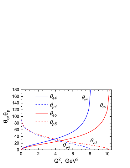
Figure 1: $Q^{2}$ dependence of the scattering angles of the electron $\theta_{e}$ and the proton $\theta_{p}$ (in degrees) at electron beam energies in the experiment Liyanage2020 . The lines $\theta_{e4}$, $\theta_{p4}$ ($\theta_{e5}$, $\theta_{p5}$) correspond to $E_{1}=4.725$ ($5.895$) GeV.

The intersection points of the lines $\theta_{e4}$ and $\theta_{p4}$ ($\theta_{e5}$ and $\theta_{p5}$) in Fig. 1 correspond to the equality $\theta_{e}=\theta_{p}$ for some values $Q^{\,2}=Q_{(ep)}^{\,2}$. At the same time $Q^{\,2}_{(ep)}=3.70\,\mbox{GeV}^{2}$ for $E_{1}=4.725$ GeV and $Q^{\,2}_{(ep)}=4.772\,\mbox{GeV}^{2}$ for $E_{1}=5.895$ GeV. For the corresponding angles we have $\theta_{ep}=30.91^{\circ}$ (0.54 rad) and $\theta_{ep}=28.45^{\circ}$ (0.50 rad).

Table 1: Electron and proton scattering angles $\theta_{e}$ and $\theta_{p}$ (in radians) in the kinematics of the experiment Liyanage2020 .

$E_{1}$ (GeV)	$Q^{2}$ (GeV2)	$\theta_{e}\,(rad)$	$\theta_{p}\,(rad)$	$Q^{2}_{max}$ (GeV)2
5.895	2.06	0.27	0.79	10.247
5.895	5.66	0.59	0.43	10.247
4.725	2.06	0.35	0.76	8.066
4.725	5.66	0.86	0.35	8.066

The data on the electron and proton scattering angles (in radians) at electron beam energies $E_{1}=4.725$ GeV and 5.895 GeV and $Q^{2}=2.06$ GeV² and 5.66 GeV² are represented in Table 1, which contains also the values of $Q^{2}_{max}$ (43) for the maximally possible $Q^{2}$ values at $E_{1}=4.725$ GeV and 5.895 GeV.

IV Polarization of a virtual photon in the $ep\to ep$ process

The $\varepsilon$ value entering into the expression for the Rosenbluth cross section (1) with the range of variation $0\leqslant\varepsilon\leqslant 1$ in modern literature, as a rule, is identified not with the degree of linear (transverse) but with the degree of longitudinal polarization of the virtual photon. Sometimes it is also referred to as the polarization parameter or simply the virtual photon polarization. The correct understanding of the physical meaning of the value $\varepsilon$ is quite rare Gakh2008 ; Alguard1976 ; Alguard1976b , but recently the number of such works has been gradually increased, see, for example, Weiss2023 ; Korchagin2021 .

The most common expression in the literature for $\varepsilon$, given on the first page, actually contains the dependence on the electron scattering angle $\theta_{e}$ in the LF. Expressions for $\varepsilon$, that make it possible to calculate the dependences of the quantities of interest on, e.g., $Q^{2}$ or the proton scattering angle $\theta_{p}$ are given by

$$\varepsilon^{-1} =1+\frac{(E_{1}-E_{2})^{2}+2(E_{1}-E_{2})\,m}{2E_{1}E_{2}-(E_{1}-E_{2})\,m}$$ (45)

$$=\frac{E_{1}^{\,2}+E_{2}^{\,2}+(E_{1}-E_{2})\,m}{2E_{1}E_{2}-(E_{1}-E_{2})\,m}\,,$$

where $E_{1}$ and $E_{2}$ are the energies of the initial and final electrons, respectively. Note that Eqs. (34) and (35) should be used for $E_{2}$, they depend explicitly only on $Q^{2}$; In turn, the $Q^{2}$ dependence on the angles of $\theta_{e}$ or $\theta_{p}$ is determined by Eqs. (38) or (40).

The $Q^{2}$ dependence of the degree of the linear polarization of the virtual photon, $\varepsilon$ (45), at electron beam energies in the SANE Collaboration experiment Liyanage2020 is represented by graphs in the Fig. 2.

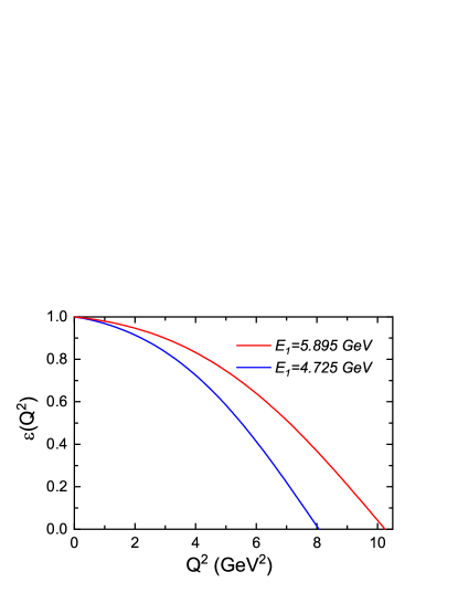
Figure 2: $Q^{2}$ dependence of the degree of the linear polarization of the virtual photon, $\varepsilon$ (45), for the electron beam energies used in the experiment Liyanage2020 .

It follows from Fig. 2 that $\varepsilon$ is a function of $Q^{2}$ and decreases from $1$ to $0$. In the case of electron scattered forward ($\theta_{e}=0^{\circ}$) when $Q^{2}=0$, $\varepsilon=1$; for a backscattered electron ($\theta_{e}=180^{\circ}$) when $Q^{2}=Q^{2}_{max}$, $\varepsilon=0$. The $Q^{2}_{max}$ values for the energies $E_{1}=4.725$ GeV and $5.895$ GeV are listed in Table 1; they amount to $8.066$ GeV² and $10.247$ GeV², respectively. Specifically at these points the lines in Fig. 2 intersect the abscissa axis.

Figure 3 shows the dependence of the degree of the linear polarization of the virtual photon, $\varepsilon$ (45), on the scattering angles of the electron $\theta_{e}$ (a) and proton $\theta_{p}$ (b) for the electron beam energies $E_{1}=4.725$ GeV and $5.895$ GeV in the experiment Liyanage2020 .

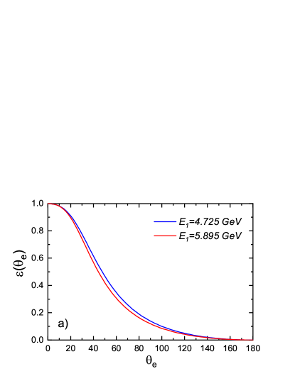
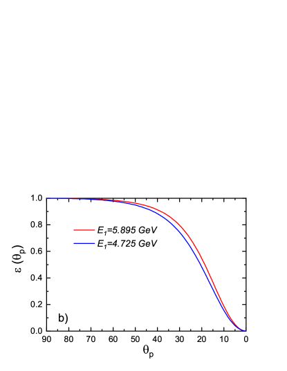
Figure 3: Angular dependence of the degree of the linear polarization of the virtual photon, $\varepsilon$ (45), on the scattering angles of the electron $\theta_{e}$ (a) and proton $\theta_{p}$ (b) expressed in degrees for the electron beam energies in the experiment Liyanage2020 .

V Polarization effects in the $e\vec{p}\to\vec{e}p$ process

V.1 Differential cross section of the $e\vec{p}\to\vec{e}p$ process

In the OPE approximation, the matrix elements of the process $e\vec{p}\to\vec{e}p$ (13) are the product of the electron $(J_{e})$ and proton currents $(J_{p})$

$$M_{ep\to ep}=4\pi\alpha\,T_{ep}/q^{2},$$ (46)

$$T_{ep}=(J_{e})^{\mu}(J_{p})_{\mu}\,.$$ (47)

The lepton $(J_{e})^{\mu}$ and proton $(J_{p})_{\mu}$ currents read:

$$(J_{e})^{\mu} = \overline{u}(p_{2})\gamma^{\mu}u(p_{1}),$$ (48)

$$(J_{p})_{\mu} = \overline{u}(q_{2})\Gamma_{\mu}(q^{2})u(q_{1}),$$ (49)

$$\Gamma_{\mu}(q^{2}) = F_{1}\gamma_{\mu}+\frac{F_{2}}{4m}(\;\hat{q}\gamma_{\mu}-\gamma_{\mu}\hat{q}\;).$$ (50)

Here $u(p_{i})$ and $u(q_{i})$ are the bispinors of electrons and protons with the 4-momenta $p_{i}$ and $q_{i}$, respectively, where $p_{i}^{2}=m_{0}^{2}$ and $q_{i}^{2}=m^{2}$, having the properties $\overline{u}(p_{i})u(p_{i})=2m_{0}$ and $\overline{u}(q_{i})u(q_{i})=2m$ $(i=1,2)$; $F_{1}$ and $F_{2}$ are the Dirac and Pauli proton form factors, respectively; $q=q_{-}=q_{2}-q_{1}$ is the 4-momentum transferred to the proton; $\hat{q}=(q)_{\mu}\gamma^{\mu}$, where $\gamma^{\mu}$ (and $\gamma^{5}$, see below) are the Dirac matrices.

It is well known that the relations

$$G_{E}=F_{1}-\tau_{p}F_{2}\,,\;G_{M}=F_{1}+F_{2},$$ (51)

translate the Dirac $F_{1}$ and Pauli $F_{2}$ form factors into the SFFs $G_{E}$ and $G_{M}$. The inverse relations are given by

$$F_{1}=\frac{G_{E}+\tau_{p}G_{M}}{1+\tau_{p}}=\frac{4m^{2}}{q_{+}^{2}}\,(G_{E}+\tau_{p}G_{M}),$$

$$F_{2}=\frac{G_{M}-G_{E}}{1+\tau_{p}}=\frac{4m^{2}}{q_{+}^{2}}\,(G_{M}-G_{E})\,.$$

For the proton vertex function $\Gamma_{\mu}(q^{2})$ (50) there are other equivalent representations that are more convenient for cross section calculations

$$\Gamma_{\mu}(q^{2}) = G_{M}\gamma_{\mu}-\frac{(q_{+})_{\mu}}{2m}\,F_{2},$$

$$\Gamma_{\mu}(q^{2}) = G_{M}\gamma_{\mu}+2m\,(G_{E}-G_{M})\,\frac{(q_{+})_{\mu}}{q_{+}^{2}}\,.$$

The differential cross section of the process (13) reads

$$\frac{d\sigma_{ep\to ep}}{dt}=\frac{\pi\alpha^{2}}{\lambda_{s}}\,\frac{|T_{ep}|^{2}}{t^{2}}\,,$$ (52)

where $\lambda_{s}=(s-(m+m_{0})^{2})(s-(m-m_{0})^{2})$ is Källén’s function.

In the standard approach AB ; BLP , the calculation of the squares of the amplitude modules $|T_{ep}|^{2}$ (47) is reduced to the convolution of the lepton ($L^{\mu\nu}$) and hadron ($H_{\mu\nu}$) tensors

$$|T_{ep}|^{2}=H_{\mu\nu}L^{\mu\nu},$$ (53)

which are expressed in terms of currents (48) and (49) as follows:

$$L^{\mu\nu}=(J_{e})^{\mu}(J_{e}^{\ast})^{\nu},\;$$

$$H_{\mu\nu}=(J_{p})_{\mu}(J_{p}^{\ast})_{\nu},$$

where the asterisk $\ast$ denotes complex conjugation.

In turn, the calculation of the tensors $L_{\mu\nu}$ and $H_{\mu\nu}$ is reduced to the operation of computing a trace from the production of the Dirac operators denoted by the symbol “Tr”

$$L^{\mu\nu}=\textmd{Tr\,}(\tau_{e_{2}}\gamma^{\mu}\tau_{e_{1}}\gamma^{\nu}),$$ (54)

$$H_{\mu\nu}=2\,\textmd{Tr\,}(\tau_{p_{2}}\,\Gamma_{\mu}\tau_{p_{1}}\,\overline{\Gamma}_{\nu})\,.~{}~{}~{}$$ (55)

Here $\tau_{e_{i}}$ and $\tau_{p_{i}}$ $(i=1,2)$ are the polarization density matrices of the initial and final states of electrons and protons ($\lambda_{p_{1}}$ and $\lambda_{e_{2}}$ are the degrees of polarization of the initial proton and the final electron and $\gamma_{5}$ is the Dirac matrix):

$$\tau_{e_{1}}=(\hat{p_{1}}+m_{0})/2,\,$$

$$\tau_{e_{2}}=(\hat{p_{2}}+m_{0})(1-\lambda_{e_{2}}\gamma_{5}\hat{s}_{e_{2}})/2\,,$$ (56)

$$\tau_{p_{1}}=(\hat{q_{1}}+m)(1-\lambda_{p_{1}}\gamma_{5}\hat{s}_{p_{1}})/2\,,$$

$$\tau_{p_{2}}=(\hat{q_{2}}+m)/2\,.$$

The lepton tensor $L^{\mu\nu}$ (54) in terms of the 4-vectors $p_{\pm}$ has the form:

$$2L^{\mu\nu} = p_{+}^{\mu}p_{+}^{\nu}-p_{-}^{\mu}p_{-}^{\nu}+p_{-}^{2}g^{\mu\nu}+2im_{0}\lambda_{e_{2}}\varepsilon^{\mu\nu\rho\sigma}(p_{-})_{\rho}(s_{e_{2}})_{\sigma}.$$

In the ultrarelativistic limit when $s_{e_{2}}=p_{2}/m_{0}$, it takes the form

$$2L^{\mu\nu} = p_{+}^{\mu}p_{+}^{\nu}-p_{-}^{\mu}p_{-}^{\nu}+p_{-}^{2}g^{\mu\nu}+i\lambda_{e_{2}}\varepsilon^{\mu\nu\rho\sigma}(p_{-})_{\rho}(p_{+})_{\sigma}.$$

The explicit form of the tensor $H_{\mu\nu}$ (55) is rather cumbersome; for this reason we omit it.

The expression for $|T_{ep}|^{2}$ (47) can be written as

$$2\,|T_{ep}|^{2}=\frac{4m^{2}}{q_{+}^{2}}|T|^{2}.$$

Since $q_{+}^{2}=4m^{2}(1+\tau_{p}$), then the differential cross section of the process (13) calculated in an arbitrary reference frame in the DSB (15), (16) takes the form

$$\frac{d\sigma_{e\vec{p}\to\vec{e}p}}{dt} = \frac{\pi\alpha^{2}}{2\lambda_{s}(1+\tau_{p})}\,\frac{|{T}|^{2}}{t^{2}},$$ (57)

$$|T|^{2} = I_{0}+\lambda_{p_{1}}\lambda_{e_{2}}I_{1},$$ (58)

$$I_{0} = G_{E}^{\,2}Y_{1}+\tau_{p}\,G_{M}^{\,2}Y_{2},$$ (59)

$$I_{1} = \tau_{p}(G_{E}G_{M}Y_{3}+G_{M}^{\,2}Y_{4}),$$ (60)

where $\lambda_{p_{1}}$ and $\lambda_{e_{2}}$ are the degrees of polarization of the initial proton and the final electron; the functions $Y_{i}$ ($i=1,\ldots 4$) are given by

$$Y_{1} = (p_{+}q_{+})^{2}+q_{+}^{2}q_{-}^{2},$$ (61)

$$Y_{2} = (p_{+}q_{+})^{2}-q_{+}^{2}(q_{-}^{2}+4m_{0}^{2}),$$ (62)

$$-Y_{3} = 2\,\kappa_{1}\,m^{2}\,((p_{+}q_{+})^{2}+q_{+}^{2}(q_{-}^{2}-4\,m_{0}^{2}\,))\,z_{1}^{2},$$ (63)

$$Y_{4} = 2(m^{2}p_{+}q_{+}-\kappa_{1}q_{+}^{2})(\kappa_{1}p_{+}q_{+}-m_{0}^{2}q_{+}^{2})z_{1}^{2},$$

$$z_{1}=(\kappa_{1}^{2}-m^{2}m_{0}^{2})^{-1/2}\,,\;\kappa_{1}=q_{1}p_{2}.$$

In the case of arbitrary spin 4-vectors $s_{p_{1}}$ and $s_{e_{2}}$, the functions $Y_{3}$ (63) and $Y_{4}$ (V.1) are given by

$$Y_{3} = 8\,m_{0}m\,(s_{p_{1}})^{\mu}(g^{\bot})_{\mu\nu}(s_{e_{2}})^{\nu}q_{+}^{2}\,,$$ (65)

$$Y_{4} = 8\,m_{0}m\,(q_{+}s_{p_{1}})(q_{+}s_{e_{2}}).$$ (66)

Note that, first, the term with $Y_{3}$ (63) in the cross section (57) is determined by the transverse part of the metric tensor $(g^{\bot})_{\mu\nu}$ (30) and contains the product of $G_{E}G_{M}$; second, in the cross section of the process $e\vec{p}\to e\vec{p}$ in DSB (8), (9) there is no similar structure, see JETPL2021 ; PEPAN2022 ; JETPL2022 .

In the ultrarelativistic limit when the mass of an electron can be neglected, expressions (61) – (V.1) for $Y_{i}$ ($i=1,\ldots 4$) are given by

$$Y_{1} = (p_{+}q_{+})^{2}+q_{+}^{2}q_{-}^{2},$$ (67)

$$Y_{2} = (p_{+}q_{+})^{2}-q_{+}^{2}\,q_{-}^{2},$$ (68)

$$-Y_{3} = 2\,m^{2}(\kappa_{1}^{-1})((p_{+}q_{+})^{2}+q_{+}^{2}q_{-}^{2}),\,$$ (69)

$$Y_{4} = 2\,p_{+}q_{+}(\kappa_{1}^{-1})(m^{2}\,p_{+}q_{+}-\kappa_{1}\,q_{+}^{2}).$$ (70)

Finally, using relations (36) for the functions $Y_{i}$ (67)–(70), we obtain expressions in the LF that depend only on the energy of the initial and final electrons:

$$Y_{1}=8m^{2}(2E_{1}E_{2}-mE_{-}),$$ (71)

$$Y_{2}=8m^{2}(E_{1}^{\,2}+E_{2}^{\,2}+mE_{-}),$$ (72)

$$Y_{3}=-(2m/E_{2})\,Y_{1},$$ (73)

$$Y_{4}=8m^{2}E_{+}E_{-}(m-E_{2})/E_{2}.$$ (74)

V.2 Polarization of the final electron in the $e\vec{p}\to\vec{e}p$ process

The expression for the square of the amplitude modulus $|T|^{2}$ (58) in the cross section (57) can be written as

$$|T|^{2}=I_{0}+\lambda_{p_{1}}\lambda_{e_{2}}I_{1}=I_{0}\,(1+\lambda_{e_{2}}\lambda_{e_{2}}^{f}).$$ (75)

Then the value $\lambda_{e_{2}}^{f}$ in (75) is the degree of longitudinal polarization transferred from the initial proton to the final electron in the $e\vec{p}\to\vec{e}p$ process:

$$\lambda_{e_{2}}^{f}=\lambda_{p_{1}}\frac{I_{1}}{I_{0}}=\lambda_{p_{1}}\frac{\tau_{p}\,(G_{E}G_{M}Y_{3}+G_{M}^{\,2}Y_{4})}{G_{E}^{\,2}Y_{1}+\tau_{p}G_{M}^{\,2}Y_{2}}.$$ (76)

Dividing the numerator and denominator in the last expression by $Y_{1}G_{M}^{\,2}$ and defining the experimentally measured ratio $R\equiv\mu_{p}G_{E}/G_{M}$, we get:

$$\lambda_{e_{2}}^{f}=\lambda_{p_{1}}\,\frac{\mu_{p}\tau_{p}\,((Y_{3}/Y_{1})R+\mu_{p}(Y_{4}/Y_{1}))}{R^{\,2}+\mu_{p}^{2}\,\tau_{p}\,(Y_{2}/Y_{1})\,}.$$ (77)

Note that for the ratio $Y_{2}/Y_{1}$ in the denominator of expression (77) in the LF, the equality $Y_{2}/Y_{1}=1/\varepsilon$ is valid, where $\varepsilon$ is the degree of linear polarization of the virtual photon (45).

Inverting relation (77), we obtain a quadratic equation with respect to $R$

$$\alpha_{0}R^{2}-\alpha_{1}R+\alpha_{0}\alpha_{3}-\alpha_{2}=0$$ (78)

with the coefficients

$$\alpha_{0}=\lambda_{e_{2}}^{f}/\lambda_{p_{1}},\;\alpha_{1}=\tau_{p}\,\mu_{p}\,Y_{3}/Y_{1},$$ (79)

$$\alpha_{2}=\tau_{p}\,\mu_{p}^{2}\,Y_{4}/Y_{1},\;\alpha_{3}=\tau_{p}\,\mu_{p}^{2}\,Y_{2}/Y_{1}.$$

Solutions to Eq. (78) read

$$R=\frac{\alpha_{1}\pm\sqrt{\alpha_{1}^{2}-4\alpha_{0}(\alpha_{0}\alpha_{3}-\alpha_{2})}}{2\alpha_{0}}.$$ (80)

They allow us to extract the ratio $R$ from the results of an experiment to measure the polarization transferred to the electron $\lambda_{e_{2}}^{f}$ in the $e\vec{p}\to\vec{e}p$ process.

V.3 Results of numerical calculations of polarization effects

Formulas (71) – (74) were used to numerically calculate the $Q^{2}$ dependence of the longitudinal polarization degree of the scattered electron $\lambda_{e_{2}}^{f}$ (77) as well as the dependence on the scattering angles of the electron and proton at electron beam energies ($E_{1}=4.725$ GeV and $5.895$ GeV) and the polarization degree of the proton target at rest ($\lambda_{p_{1}}=P_{t}=0.70$) in the experiment Liyanage2020 while conserving the scaling of the SFFs in the case of a dipole dependence $R=R_{d}$ ($R_{d}=1$), and in the case of its violation. In the latter case, the parametrization $R=R_{j}$ from the paper Qattan2015 was used

$$R_{j}=(1+0.1430\,Q^{2}-0.0086\,Q^{4}+0.0072\,Q^{6})^{-1},$$ (81)

and also the Kelly parametrization ($R=R_{k}$) from Kelly2004 formulas for which we omit.

The calculation results are presented by graphs in Figs. 4 and 5. Note that in these figures there are no lines corresponding to the parametrization Kelly2004 since calculations using $R_{j}$ and $R_{k}$ give almost identical results.

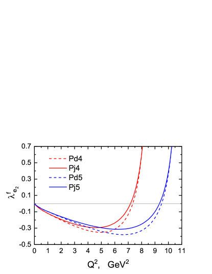
Figure 4: $Q^{2}$ dependence of the longitudinal polarization degree of the scattered electron $\lambda_{e_{2}}^{f}$ (77) at electron beam energies in the experiment Liyanage2020 . The lines $Pd4$, $Pd5$ (dashed) and $Pj4$, $Pj5$ (solid) correspond to the ratio $R=R_{d}$ and $R=R_{j}$ (81). The lines $Pd4$, $Pj4$ ($Pd5$, $Pj5$) correspond to the energies $E_{1}=4.725$ ($5.895$) GeV.

The $Q^{2}$ dependence of the longitudinal polarization degree of the scattered electron $\lambda_{e_{2}}^{f}$ (77) is plotted in Fig. 4, on which the lines $Pd4$, $Pd5$ (dashed) and $Pj4$, $Pj5$ (solid) are constructed for $R=R_{d}$ and $R=R_{j}$ (81). At the same time, the red lines $Pd4$, $Pj4$ and the blue lines $Pd5$, $Pj5$ correspond to the energy of the electron beam $E_{1}=4.725$ GeV and $5.895$ GeV. For all lines in Fig. 4 the degree of polarization of the proton target at rest $P_{t}=0.70$.

As can be seen from the graphs in Fig. 4, the function $\lambda_{e_{2}}^{f}(Q^{2})$ (77) takes negative values for most of the allowed values $Q^{2}$ and has a minimum for some of them, we will specify them: $Pd4(4.976)=-0.352$, $Pj4(4.586)=-0.294$, $Pd5(6.648)=-0.380$, $Pj5(6.254)=-0.314$. We also give the values for $Q^{2}$, at which the lines in the Fig. 4 intersect with the abscissa axis (begin to take positive values): $Pj4(7.174)=0$, $Pd4(7.340)=0$, $5(9.333)=0$, $Pd5(9.492)=$0. Thus, in a smaller part of the allowed values adjacent to $Q^{2}_{max}$ and amounting to approximately 9% of $Q^{2}_{max}$, the function $\lambda_{e_{2}}^{f}(Q^{2})$ takes positive values. At the boundary of the spectrum at $Q^{2}=Q^{2}_{max}$, the polarization transferred to the electron is equal to the polarization of the proton target, $\lambda_{e_{2}}^{f}(Q^{2}_{max})=P_{t}=0.70$.

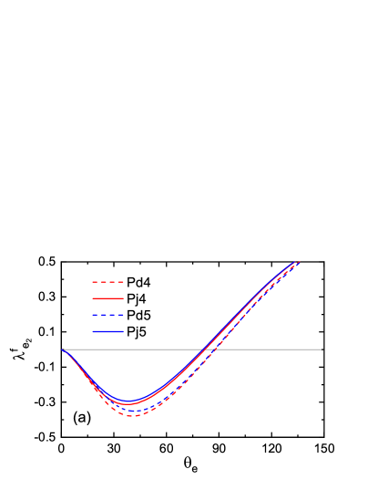
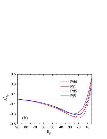
Figure 5: Angular dependence of the degree of the transferred to the electron polarization $\lambda_{e_{2}}^{f}$ (77) at electron beam energies used in the experiment Liyanage2020 on the scattering angle of the electron $\theta_{e}$ (a) and of the proton $\theta_{p}$ (b), expressed in degrees. The marking of lines $Pd4$, $Pd5$, $Pj4$, $Pj5$ is the same as in Fig. 4.

The results of calculations of the angular dependence of the polarization transferred to the electron $\lambda_{e_{2}}^{f}$ (77) in the $e\vec{p}\to\vec{e}p$ process at electron beam energies $E_{1}=4.725$ GeV and $E_{1}=5.895$ GeV in the experiment Liyanage2020 as functions of the scattering angle of the electron ($\theta_{e}$) and proton ($\theta_{p}$) are represented by graphs in Fig. 5. The degree of polarization of the proton target for all lines was taken to be the same and equal to $P_{t}=0.70$. The figures (a) and (b) represent the dependence on the scattering angle of the electron $\theta_{e}$ and proton $\theta_{p}$, respectively.

Obviously, the behavior of the lines in Fig. 5 for the angular dependence is similar to the behavior of the lines for the $Q^{2}$ dependence in Fig. 4.

Using the QattanQattan2015 and Kelly Kelly2004 parametrizations, the relative difference $\Delta_{dj}$ between the polarization effects in the process of $e\vec{p}\to\vec{e}p$ was calculated in the case of conservation and violation of the scaling of the SFFs as well as in the effects between these parameterizations $\Delta_{jk}$

$$\Delta_{dj}=\Big{|}\frac{\rm{Pd}-\rm{Pj}}{\rm{Pd}}\Big{|},\;\Delta_{jk}=\Big{|}\frac{\rm{Pj}-\rm{Pk}}{\rm{Pj}}\Big{|},$$ (82)

where $P_{d}$, $P_{j}$, and $P_{k}$ are the polarizations calculated by formula (77) for $\lambda_{e_{2}}^{f}$ when using the corresponding parametrizations $R_{d}$, $R_{j}$, and $R_{k}$. The results of calculations of $\Delta_{dj}$ at electron beam energies of $4.725$ GeV and $5.895$ GeV are shown in Fig. 6.

Table 2: The degree of longitudinal polarization of the scattered electron $\lambda_{e_{2}}^{f}$ (77) at $E_{1}$ and $Q^{2}$ used in the experiment Liyanage2020 . The values in the columns for $P_{d}$, $P_{j}$, and $P_{k}$ correspond to dipole dependence and the Qattan Qattan2015 and Kelly Kelly2004 parametrization (81). The corresponding electron and proton scattering angles (in degrees) are given in columns for $\theta_{e}$ and $\theta_{p}$.

$E_{1}$, GeV	$Q^{2}$, GeV2	$\theta_{e}\,(^{\circ})$	$\theta_{p}\,(^{\circ})$	$P_{d}$	$P_{j}$	$P_{k}$	$\Delta_{dj}$, %	$\Delta_{jk}$, %
5.895	2.06	15.51	45.23	–0.170	–0.163	–0.163	4.1	0.0
5.895	5.66	33.57	24.48	–0.363	–0.309	–0.308	14.9	0.3
4.725	2.06	19.97	43.27	–0.207	–0.197	–0.197	4.8	0.0
4.725	5.66	49.50	19.77	–0.336	–0.263	–0.262	21.7	0.6

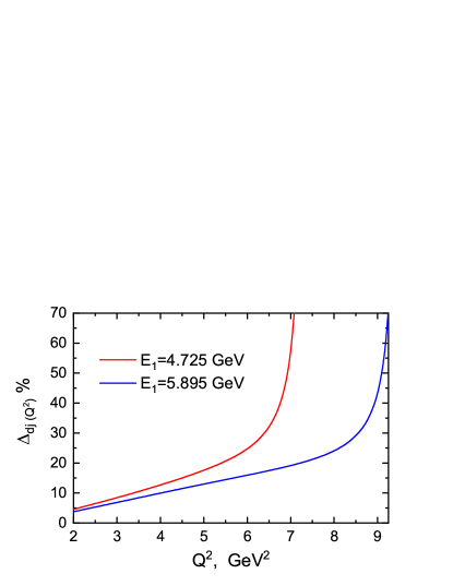
Figure 6: $Q^{2}$ dependence of the relative difference $\Delta_{dj}$ (82) at electron beam energies $E_{1}=4.725~{}\mbox{GeV}$ (red line) and $E_{1}=5.895~{}\mbox{GeV}$ (blue line). For all lines, the degree of polarization of the proton target was taken to be the same $P_{t}=0.70$.

It follows from the graphs in Fig. 6 that the relative difference between the polarization transferred from the initial proton to the final electron in the $e\vec{p}\to\vec{e}p$ process in the case of conservation and violation of the scaling of the SFFs can reach 70%, which can be used to set up a polarization experiment by measuring the ratio $R$.

Numerical values of the polarization transferred to the final electron in the $e\vec{p}\to\vec{e}p$ process for the three considered parametrizations of the ratio $R$ at $E_{1}$ and $Q^{2}$ used in the experiment Liyanage2020 , are represented in Table 2. In it, the columns of values $P_{d}$, $P_{j}$, and $P_{k}$ correspond to the dipole dependence $R_{d}$, parametrizations $R_{j}$ (81) from Qattan2015 and $R_{k}$ Kelly2004 ; the columns $\Delta_{dj}$, $\Delta_{jk}$ correspond to the relative difference (82) (expressed in percent) at electron beam energies of $4.725$ GeV and $5.895$ GeV and two values of $Q^{2}$ equal to $2.06~{}\mbox{GeV}^{2}$ and $5.66~{}\mbox{GeV}^{2}$. It follows from Table 2 that the relative difference between $Pj5$ and $Pd5$ at $Q^{2}=2.06~{}\mbox{GeV}^{2}$ is 4.1% and between $Pj4$ and $Pd4$ it is 4.8%. At $Q^{2}=5.66~{}\mbox{GeV}^{2}$, the difference increases and becomes equal to 14.9 % and 21.7%, respectively. Note that the relative difference $\Delta_{jk}$ between $P_{j}$ and $P_{k}$ for all $E_{1}$ and $Q^{2}$ in Table 2 is less than 1%.

VI Polarization effects in the $\vec{e}\vec{p}\to ep$ process

VI.1 Cross section of the $\vec{e}\vec{p}\to ep$ process

In the OPE approximation, the differential cross section of the process (20), calculated in an arbitrary reference frame in DSB (22), (23) read

$$\frac{d\sigma_{\vec{e}\vec{p}\to ep}}{dt} = \frac{\pi\alpha^{2}}{\lambda_{s}(1+\tau_{p})}\,\frac{|{T}|^{2}}{t^{2}},$$ (83)

$$|T|^{2} = I_{0}+\lambda_{e_{1}}\lambda_{p_{1}}I_{1},$$ (84)

$$I_{0} = G_{E}^{\,2}Y_{1}+\tau_{p}\,G_{M}^{\,2}Y_{2},$$ (85)

$$I_{1} = \tau_{p}(G_{E}G_{M}Y_{3}+G_{M}^{\,2}Y_{4}),$$ (86)

where $\lambda_{e_{1}}$ and $\lambda_{p_{1}}$ are the degrees of polarization of the initial electron and proton, and the functions $Y_{i}$ ($i=1,\ldots 4$) read

$$Y_{1} = (p_{+}q_{+})^{2}+q_{+}^{2}q_{-}^{2},$$ (87)

$$Y_{2} = (p_{+}q_{+})^{2}-q_{+}^{2}(q_{-}^{2}+4m_{0}^{2}),$$ (88)

$$-Y_{3} = 2\kappa_{2}\,m^{2}((p_{+}q_{+})^{2}+q_{+}^{2}(q_{-}^{2}-4\,m_{0}^{2}\,))\,z_{2}^{2},$$ (89)

$$Y_{4} = 2(m^{2}p_{+}q_{+}-\kappa_{2}q_{+}^{2})(\kappa_{2}p_{+}q_{+}-m_{0}^{2}q_{+}^{2})z_{2}^{2},$$

$$z_{2}=(\kappa_{2}^{2}-m^{2}m_{0}^{2})^{-1/2}\,,\;\kappa_{2}=q_{1}p_{1}.$$

In the case of arbitrary spin 4-vectors $s_{e_{1}}$ and $s_{p_{1}}$, the expressions for $Y_{3}$ (89) and $Y_{4}$ (VI.1) have the form:

$$Y_{3} = 8\,m_{0}m\,(s_{p_{1}})^{\mu}(g^{\bot})_{\mu\nu}(s_{e_{1}})^{\nu}q_{+}^{2}\,,$$ (91)

$$Y_{4} = 8\,m_{0}m\,(q_{+}s_{p_{1}})(q_{+}s_{e_{1}}).$$ (92)

Note, first, that the polarized part of the cross section (83) includes the term with $Y_{3}$ (89) containing the product of the SFFs, $G_{E}G_{M}$, and according to (91), is determined by the transverse part of the metric tensor $(g^{\bot})_{\mu\nu}$ (30). Second, there is no similar structure in the cross section of the $e\vec{p}\to e\vec{p}$ process in the DSB (8), (9), see JETPL2021 ; PEPAN2022 ; JETPL2022 .

In the ultrarelativistic massless limit, the expressions (87) – (VI.1) for $Y_{i}$ ($i=1,\ldots 4$) are given by

$$Y_{1} = (p_{+}q_{+})^{2}+q_{+}^{2}q_{-}^{2},$$ (93)

$$Y_{2} = (p_{+}q_{+})^{2}-q_{+}^{2}\,q_{-}^{2},$$ (94)

$$-Y_{3} = 2\,m^{2}(\kappa_{2}^{-1})((p_{+}q_{+})^{2}+q_{+}^{2}q_{-}^{2}),\,$$ (95)

$$Y_{4} = 2\,p_{+}q_{+}(\kappa_{2}^{-1})(m^{2}\,p_{+}q_{+}-\kappa_{2}\,q_{+}^{2}).$$ (96)

Finally, using relations (36) for the functions $Y_{i}$ (93)–(96) in the LF, we obtain expressions that depend only on the energies of the initial and final electrons $E_{1}$ and $E_{2}$:

$$Y_{1} = 8m^{2}(2E_{1}E_{2}-mE_{-}),$$ (97)

$$Y_{2} = 8m^{2}(E_{1}^{\,2}+E_{2}^{\,2}+mE_{-}),$$ (98)

$$-Y_{3} = (2m/E_{1})\,Y_{1},$$ (99)

$$-Y_{4} = 8m^{2}E_{+}E_{-}(m+E_{1})/E_{1}.$$ (100)

The polarization asymmetry in the process (20) is determined by the square of the amplitude modulus (84) as follows Alguard1976 ; Alguard1976b :

$$A=\frac{|{T}|^{2}(\lambda_{e_{1}}=-1)-|{T}|^{2}(\lambda_{e_{1}}=+1)}{|{T}|^{2}(\lambda_{e_{1}}=-1)+|{T}|^{2}(\lambda_{e_{1}}=+1)}.$$ (101)

As a result we have

$$A=-\lambda_{p_{1}}\frac{\tau_{p}\,(G_{E}G_{M}Y_{3}+G_{M}^{\,2}Y_{4})}{G_{E}^{\,2}Y_{1}+\tau_{p}G_{M}^{\,2}Y_{2}}.$$ (102)

By dividing the numerator and denominator in the last expression into $G_{M}^{\,2}$ and defining the experimentally measured ratio $R\equiv\mu_{p}G_{E}/G_{M}$, we get:

$$A=-\lambda_{p_{1}}\,\frac{\mu_{p}\tau_{p}\,((Y_{3}/Y_{1})R+\mu_{p}(Y_{4}/Y_{1}))}{R^{\,2}+\mu_{p}^{2}\,\tau_{p}\,(Y_{2}/Y_{1})\,}.$$ (103)

Note that expressions (102), (103) for polarization asymmetry in the $\vec{e}\vec{p}\to ep$ process and the expressions (76), (77) for electron transferred polarization $\lambda_{e_{2}}^{f}$ in the $e\vec{p}\to\vec{e}p$ process coincide up to the sign. For this reason, the quadratic equation for extracting the ratio $R$ coincides with the explicit form of equation (78) and has coefficients of the same shape, except for one: $\alpha_{0}=-A_{exp}/\lambda_{p_{1}}$, where $A_{exp}$ is experimentally measured polarization asymmetry.

The results of numerical calculations of the $Q^{2}$ dependence of the polarization asymmetry $A$ (103) in the $\vec{e}\vec{p}\to ep$ process at electron beam energies $E_{1}=4.725$ GeV and 5.895 GeV are represented by graphs in the Fig. 7, from which it follows that this dependence for each of the energies of the electron beam is almost linear. With increasing of $Q^{2}$ from 0 to $Q^{2}_{max}$, it changes from 0 to $P_{t}=0.70$ at the boundaries of the spectrum at $Q^{2}=Q^{2}_{max}$. The effects of scaling violations are small in the entire range of acceptable values of $Q^{2}$; they do not exceed 1.79 % at $E_{1}=4.725$ GeV and 2.32 % at $E_{1}=5.895$ GeV. For this reason, the measurement of polarization asymmetry in the $\vec{e}\vec{p}\to ep$ process can be used as a test to verify the conservation of the SFF scaling.

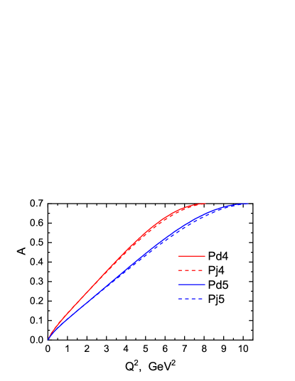
Figure 7: $Q^{2}$ dependence of the polarization asymmetry of $A$ (103) in the $\vec{e}\vec{p}\to ep$ process at electron beam energies in the experiment Liyanage2020 . The lines $Pd4,Pd5$ (solid) and $Pj4,Pj5$ (dashed) correspond to the dipole dependence $R=R_{d}$ ($R_{d}=1$) and parametrization of $R=R_{j}$ (81) from Qattan2015 . The lines $Pd4,Pj4$ ($Pd5,Pj5$) correspond to the electron beam energy $4.725$ GeV and $5.895$ GeV. For all lines, the degree of polarization of the proton target was taken to be the same $P_{t}=0.70$.

Note that the double spin asymmetry in the elastic process $\vec{e}\vec{p}\to ep$ in the case when the spin quantization axes of a resting proton target and an incident electron beam are parallel was first measured in the experiment Alguard1976 , as a result of which it was first established that the SFF ratio $R$ is positive.

VII Conclusion

In this paper, in the one-photon exchange approximation we analyze polarization effects in the elastic $\vec{e}\vec{p}\to ep$ and $e\vec{p}\to\vec{e}p$ processes in the case when the spin quantization axes of the target proton at rest and the incident or scattered electron are parallel. To do this, in the kinematics of the SANE Collaboration experiment Liyanage2020 using the Kelly Kelly2004 and Qattan Qattan2015 parametrizations for the Sachs form factor ratio $R\equiv\mu_{p}G_{E}/G_{M}$, a numerical analysis was carried out of the dependence of the longitudinal polarization degree transferred to the scattered electron in the $e\vec{p}\to\vec{e}p$ process and the double spin asymmetry in the $\vec{e}\vec{p}\to ep$ process on the square of the momentum transferred to the proton as well as on the scattering angle of the electron. As it turned out, the Qattan Qattan2015 and Kelly Kelly2004 parametrizations give almost identical results.

As a result of calculations, it was established that the relative difference in the longitudinal polarization degree of the final electron in the $e\vec{p}\to\vec{e}p$ process for the case of conservation and violation of the SFF scaling can reach 70 %, which can be used to conduct a polarization experiment of a new type of measurement of the SFF ratio $R$.

For the double spin asymmetry in the $\vec{e}\vec{p}\to ep$ process this difference is rather small and does not exceed 1.79 % for the electron beam energy $E_{1}=4.725$ GeV and 2.32 % for $E_{1}=5.895$ GeV. For this reason, the measurement of polarization asymmetry in the $\vec{e}\vec{p}\to ep$ process can be used as a test to verify the conservation of the SFF scaling.

At present, the experiment on measuring the degree of longitudinal polarization transferred to the final electron in the process $e\vec{p}\to\vec{e}p$ seems to be quite realistic, since a proton target with a high degree of polarization $P_{t}=70\pm 5$ % has been already created and is used in the experiment Liyanage2020 . For this reason, it would be most appropriate to conduct the proposed experiment at the setup used in Liyanage2020 at the same proton polarization degree $P_{t}=0.70$, electron beam energies $E_{1}=4.725$ GeV and 5.895 GeV.

The difference between the proposed experiment and the one in Liyanage2020 consists in the fact that an incident electron beam must be unpolarized, and the detected scattered electron must move strictly along the direction of the spin quantization axis of a resting proton target. In the proposed experiment, it is necessary to measure only the longitudinal polarization degree of the scattered electron,which is an advantage compared to the AR method Rekalo74 used in JLab polarization experiments.

References

- (1) R. Hofstadter, F. Bumiller, and M. R. Yearian, Rev. Mod. Phys. 30, 482 (1958).
- (2) M. N. Rosenbluth, Phys. Rev. 79, 615 (1950).
- (3) N. Dombey, Rev. Mod. Phys. 41, 236 (1969).
- (4) A. I. Akhiezer and M. P. Rekalo, Sov. J. Part. Nucl. 4, 277 (1974) (Phys. Element. Chastits Atom. Yadra. 4, 662 (1973) [in Russian]).
- (5) A. I. Akhiezer and M. P. Rekalo, Electrodynamics of Hadrons (Naukova Dumka, Kiev, 1977) [in Russian].
- (6) M. V. Galynskii and M. I. Levchuk, Phys. At. Nucl. 60, 1855 (1997) (Yad. Fiz. 60, 2028 (1997) [in Russian]).
- (7) S. Pacetti, R. Baldini Ferroli, and E. Tomasi-Gustafsson, Phys. Rept. 550-551, 1 (2015).
- (8) V. Punjabi, C. F. Perdrisat, M. K. Jones, E. J. Brash, and C. E. Carlson, Eur. Phys. J. A 51, 79 (2015).
- (9) Y. S. Liu and G. A. Miller, Phys. Rev. C 92, 035209 (2015).
- (10) M. K. Jones, K. A. Aniol, F. T. Baker, et al., Phys. Rev. Lett. 84, 1398 (2000).
- (11) O. Gayou, K. Wijesooriya, A. Afanasev et al., Phys. Rev. C 64, 038202 (2001).
- (12) O. Gayou, K. A. Aniol, T. Averett et al., Phys. Rev. Lett. 88, 092301 (2002).
- (13) V. Punjabi, C.F. Perdrisat, K.A. Aniol, et al., Phys. Rev. C 71, 055202 (2005).
- (14) A. J. R. Puckett, E. J. Brash, M. K.Jones et al., Phys. Rev. Lett. 104, 242301 (2010).
- (15) A. J. R. Puckett, E. J. Brash, O. Gayou et al., Phys. Rev. C 85, 045203 (2012).
- (16) A. J. R. Puckett, E. J. Brash, M. K. Jones et al., Phys. Rev. C 96, 055203 (2017).
- (17) I. A. Qattan, J. Arrington, R. E. Segel et al., Phys. Rev. Lett. 94, 142301 (2005).
- (18) A. Liyanage, W. Armstrong, H. Kang et al., Phys. Rev. C 101, 035206 (2020).
- (19) T. W. Donnelly and A. S. Raskin, Ann. Phys. 169, 247 (1986).
- (20) M. V. Galynskii, E. A. Kuraev, and Yu. M. Bystritskiy, JETP Lett. 88, 481 (2008), arXiv:0805.0233 [hep-ph].
- (21) M. V. Galynskii, JETP Lett. 109, 1 (2019), arXiv: 1910.05267 [hep-ph].
- (22) M. V. Galynskii and R. E. Gerasimov, JETP Lett. 110, 646 (2019), arXiv:2004.07896 [hep-ph].
- (23) M. V. Galynskii, JETP Lett. 113, 555 (2021), arXiv:2107.08503 [hep-ph].
- (24) M. V. Galynskii, Phys. Part. Nucl. Lett. 19, 26 (2022), arXiv:2112.12022 [nucl-ex].
- (25) M. V. Galynskii, JETP Lett. 116, 420 (2022) arXiv:2212.13431 [hep-ph].
- (26) M. V. Galynskii, Yu. M. Bystritskiy, and V. M. Galynsky, Phys. Rev. D 108, 096032 (2023).
- (27) J. J. Kelly, Phys. Rev. C 70, 068202 (2004).
- (28) I. A. Qattan, J. Arrington, and A. Alsaad, Phys. Rev. C 91, 065203 (2015).
- (29) M. Jacob and G. Wick, Ann. Phys. 7, 404 (1959).
- (30) F. I. Fedorov, Theor. Math. Phys. 2, 248 (1970).
- (31) F. I. Fedorov, The Lorentz Group (Nauka, Moscow, 1979) [in Russian].
- (32) A. I. Akhiezer and V. B. Berestetskii, Quantum Electrodynamics, 3rd ed. (Nauka, Moscow, 1969; Wiley, New York, 1965).
- (33) V. B. Berestetskii, E. M. Lifshits, and L. P. Pitaevskii, Course of Theoretical Physics, Vol. 4: Quantum Electrodynamics (Nauka, Moscow, 1989; Pergamon, Oxford, 1982).
- (34) S. M. Sikach, Vesti Akad. Nauk BSSR, Ser. Fiz. Mat. Nauk, 2, 84 (1984) [in Russian].
- (35) M. V. Galynskii, S. M. Sikach, Phys. Part. Nucl. 29, 469 (1998).
- (36) G. I. Gakh, E. Tomasi-Gustafsson, Nucl. Phys. A 799, 127 (2008).
- (37) M. J. Alguard et al. Phys. Rev. Lett. 37, 1258 (1976).
- (38) M. J. Alguard et al. Phys. Rev. Lett. 37, 1261 (1976).
- (39) N. Korchagin, and A. Radzhabov, arXiv: 2106.06883 [nucl-th].
- (40) F. Gil-Dominguez, J. Alarcon, C. Weiss, Phys. Rev D 108, 074026 (2023).