Silent Orbits and Cancellations in the Wave Trace

Abstract.

This paper shows that the wave trace of a bounded and strictly convex planar domain may be arbitrarily smooth in a neighborhood of some point in the length spectrum. In other words, the Poisson relation, which asserts that the singular support of the wave trace is contained in the closure of $\pm$ the length spectrum, can almost be made into a strict inclusion. To do so, we construct large families of domains for which there exist multiple periodic billiard orbits having the same length but different Maslov indices. Using the microlocal Balian-Bloch-Zelditch parametrix for wave invariants developed in our previous paper, we solve a large system of equations for the boundary curvature jets, which leads to the required cancellations. We call such periodic orbits silent, since they are undetectable from the ostensibly audible wave trace. Such cancellations show that there are potential limitations in using the wave trace for inverse spectral problems and more fundamentally, that the Laplace spectrum and length spectrum are inherently different mathematical objects, at least insofar as the wave trace is concerned.

1. Main results

In basic Fourier analysis, the Poisson summation formula on $\mathbb{R}$ can be written as

(1) $$\sum_{k\in\mathbb{N}}\cos kt=-\frac{1}{2}+\pi\sum_{j\in\mathbb{Z}}\delta_{2\pi j}(t),$$

in the sense of distributions. If one observes that $-\partial_{t}^{2}\cos(kt)=k^{2}\cos(kt)$, the lefthand side of 1 can be interpreted as the “wave trace,” $\text{Tr}\,\cos(t\sqrt{-\partial_{t}^{2}})$, which is a spectral quantity. The righthand side of 1 is a sum of distributions with singular support at multiples of $2\pi$, which are exactly the periods of closed geodesics on the circle $\mathbb{R}/2\pi\mathbb{Z}$. These, by contrast, are geometric in nature. In particular, the Poisson summation formula on the circle implies the Poisson relation: the singular support of the wave trace is contained in $\pm$ the lengths of closed geodesics. Now denote by $\Omega$ a bounded, smooth and strictly convex planar domain and consider the eigenvalue problem for the Laplacian with Dirichlet boundary conditions:

$$\begin{cases}-\Delta u_{j}=\lambda_{j}^{2}u_{j},\\ u_{j}\big{|}_{\partial\Omega}=0.\end{cases}$$

The even wave trace is defined by

$$w(t):=\text{Tr}\,\cos t\sqrt{-\Delta}=\sum_{j=1}^{\infty}\cos(t\lambda_{j}),$$

again to be interpreted in the sense of distributions. The Poisson relation, in this setting due to Anderson and Melrose [AM77]), connects the singular support of $w(t)$ to the length spectrum of $\Omega$:

(2) $$\text{SingSupp }w(t)\subset\left\{0\right\}\cup\pm\overline{\text{LSP}(\Omega)},$$

where $\text{LSP}(\Omega)$ consists of the lengths of all periodic billiard trajectories in $\Omega$. As before, the beauty of 2 is that the lefthand side is entirely spectral whereas the righthand side is geometric. However, in principle, the wave trace need not be singular at every point of length spectrum, which leads us to our main result:

Theorem 1.1.

Denote by $\mathcal{E}_{e}$ an ellipse of eccentricity $e$. For any $0\leq e<1$ and $N\in\mathbb{N}$, there exist arbitrarily $C^{\infty}$-small deformations $\Omega$ of $\mathcal{E}_{e}$ such that for some $L$ in the length spectrum of $\Omega$, $w_{\Omega}(t)$ is locally $C^{N}$ near $L$.

1.1. Wave invariants

We now establish the trace formula which leads to Theorem 1.1. Let $L$ be isolated in $\text{LSP}(\Omega)$ with finite multiplicity and assume that all corresponding periodic orbits are nondegenerate. To study the smoothness of $w(t)$ locally near a length $L$, choose $\widehat{\rho}\in C_{c}^{\infty}$ to be identically equal to $1$ in a neighborhood of $L$ and satisfy $\text{supp}(\widehat{\rho})\cap\text{LSP}(\Omega)=L$. We then have an asymptotic expansion of the form

(3) $$\int_{0}^{\infty}\widehat{\rho}(t)w(t)e^{i\lambda t}dt\sim\sum_{\gamma:\text{length}(\gamma)=L}\mathcal{D}_{\gamma}\sum_{j=0}^{\infty}B_{j,\gamma}\lambda^{-j},$$

as $\operatorname{Re}\lambda\to\infty$, where the righthand side is a sum over all periodic orbits $\gamma$ having length $L$. We call $\mathcal{D}_{\gamma}$ the symplectic prefactor and $B_{j,\gamma}$ the Balian-Bloch-Zelditch (BBZ) wave invariants.

As the BBZ expansion involves a sum over all periodic orbits having length $L$, their contributions to (3) may interfere destructively and cause cancellations. This is the approach we take in proving Theorem 1.1. Since the decay of a function is equivalent to smoothness of its Fourier transform, if the invariants $B_{j,\gamma}$ sum (over $\gamma$) to $0$ for each $j=1,2,\cdots,m$, then the series (3) will be $O(k^{-m-1})$ and $w(t)$ will be locally $C^{m-1}$. If they sum to zero for all $j\in\mathbb{N}$, then the wave trace will be locally $C^{\infty}$. In our previous paper [KKV24], we derived formulae for $\mathcal{D}_{\gamma}$ and $B_{j,\gamma}$ in terms of the length functional (see (7)) when $\gamma$ is a “nearly degenerate” periodic orbit. Note that in Theorem 1.1, $\Omega$ is a deformation of an ellipse, the integrability of which guarantees that periodic orbits in $\Omega$ will be nearly degenerate in the sense of [KKV24]. Deriving formulae for the Balian-Bloch-Zelditch invariants there used primarily microlocal methods, whereas here, we employ dynamical techniques to orchestrate cancellations amongst them.

1.2. Outline of the proof

We aim to show that for some $L$ which is isolated in the length spectrum of a domain $\Omega$, we have

(4) $$\sum_{\gamma:\text{length}(\gamma)=L}\mathcal{D}_{\gamma}B_{j,\gamma}=0,\;\;\;\forall j=0,1,\ldots,m.$$

The symplectic prefactor $\mathcal{D}_{\gamma}$ in (3) has an oscillatory part $\exp ikL$ together with an additional complex phase, $\exp i\pi m_{\gamma}/4$, where $m_{\gamma}$ is the Maslov index of $\gamma$ (see Theorem 3.10). To create cancellations, we begin with an ellipse and deform it in such a way that the Maslov indices of two families of periodic orbits in our new domain differ by $4\mod 8$. This way, the complex exponential for one family is the negative of another. At the level of geometry, this can be arranged by ensuring that each family of periodic orbits have distinct rotation numbers in the new domain and have varying ellipticity/hyperbolicity. Since the invariants $B_{j,\gamma}$ are in fact complex valued, we actually need $4$ families, corresponding to the phases $\pm 1$ and $\pm i$. The additional phases are created by separating out elliptic and hyperbolic orbits. The technicalities of how we can select sufficiently many orbits of a fixed length $L$, prescribe their ellipticity/hyperbolicity together with opposite Maslov factors, all while ensuring that no additional periodic orbits of length $L$ emerge in the deformation, is outlined below.

Step 1. Start with an ellipse $\mathcal{E}_{e}$ of eccentricity $e$ and choose two rational caustics, $\Gamma$ and $\Gamma^{\prime}$, which have distinct rotation numbers $p/q$ and $p^{\prime}/q^{\prime}$, but are such that all corresponding tangent billiard orbits have the same length $L$. Not every ellipse has a pair of such caustics. In fact, the set of eccentricites for which this happens has Lebesgue measure zero (see Remark 5.6). However, using elliptic integrals and tools from Aubry-Mather theory, in particular Mather’s $\beta$ function, we show that there is in fact a dense set of eccentricities $e\in[0,1)$ for which there exist at least two such caustics; see Theorem 5.5. We call this situation a length spectral resonance.

Step 2. Select a family $\mathcal{F}_{m}$ consisting of $4m$ distinct periodic orbits in $\mathcal{E}_{e}$, all of which have length $L$, such that $2m$ of them are tangent to the caustic $\Gamma$ and the other $2m$ are tangent to $\Gamma^{\prime}$. It is clear that each of these orbits is degenerate. We will smoothly deform $\mathcal{E}_{e}$ while preserving both convexity and first order contact at the $2m(q+q^{\prime})$ reflection points of the $4m$ orbits in $\mathcal{F}_{m}$.

Step 3. Let $\bar{\varepsilon},\bar{\delta}\in\mathbb{R}^{4m}$ be small perturbation parameters and denote by $n_{x}\in\mathbb{R}^{2}$ the outward pointing unit normal vector to $\mathcal{E}_{e}$ at the point $x\in\mathcal{E}_{e}$. We introduce a multiscale family of deformations of $\mathcal{E}_{e}$, which we denote by

$$\Omega_{\bar{\varepsilon},\bar{\delta}}:=\left\{x+\mu_{\bar{\varepsilon},\bar{\delta}}(x)n_{x}:x\in\mathcal{E}_{e}\right\},$$

shortened to $\Omega$ moving forward, where $\mu_{\bar{\varepsilon},\bar{\delta}}$ is a smooth $8m$-parameter family of functions. We insist that the deformation preserve all orbits from $\mathcal{F}_{m}$ in the sense described above. $\mathcal{F}_{m}$ remains a family of periodic orbits in $\Omega$ which have length $L$ and they will be nearly degenerate in the sense of [KKV24]. We can deform in such a way that of the $2m$ type-$(p,q)$ orbits which are tangent to $\Gamma$, $m$ of them become elliptic and $m$ of them become hyperbolic. Similarly, we can deform so that $m$ of the orbits tangent to $\Gamma^{\prime}$ become elliptic while $m$ become hyperbolic. Suppose we can arrange for such perturbations to destroy all other periodic orbits of length $L$; this is in fact the main difficulty in Section 6. This combination of ellipticity and hyperbolicity will then generate all $4$ different Maslov factors mentioned above.

Step 4. Let $\ell=|\partial\Omega|$ and denote by $ds$ the arclength measure along $\partial\Omega$. If $x:\mathbb{R}/\ell\mathbb{Z}:=\mathbb{T}_{\ell}\to\mathbb{R}^{2}$ is an arclength parametrization of $\partial\Omega$, we denote the parametrization of $\partial\Omega^{q}$ by $x(S)\in\mathbb{R}^{2q}$ with $S=(s_{1},\cdots,s_{q})\in\mathbb{T}_{\ell}^{q}$ and $x_{i}(S)$ being the $(x_{i}^{1},x_{i}^{2})$ coordinates, $i\in\mathbb{Z}/q\mathbb{Z}$. The length functional is defined by

$$\mathcal{L}(S)=\sum_{i=1}^{q}|x_{i+1}(S)-x_{i}(S)|.$$

The BBZ wave invariants $B_{j,\gamma}$ are calculated in [KKV24] by applying the method of stationary phase to an oscillatory integral representation of the lefthand side of equation 3. This oscillatory integral has the form

$$\int_{0}^{\infty}e^{ikt}\widehat{\rho}(t)w(t)dt=\int_{\mathbb{T}_{\ell}^{q}}e^{ik\mathcal{L}(S)}a_{0}(S;k)dS,$$

where $a_{0}$ is an amplitude depending on the lengths of links $\overline{x_{i}(S)x_{i+1}(S)}$ for any $q$-link configuration in $\partial\Omega^{q}$. In order to match the $B_{\gamma,j}$ coefficients in Theorem 1 of [KKV24] (Theorem 3.10 below), we must prescribe the length functional’s jet at reflection points on the boundary. To do so, it is sufficient to deform the curvature of the boundary together with its first derivative. The necessary $q$ and $q^{\prime}$-fold curvature jets will be obtained as the solution to a large system of equations associated to all $2m(q+q^{\prime})$ points of reflection.

Step 5. Upon deforming $\mathcal{E}_{e}$, we may create additional orbits which now share the same length $L$, where we are trying to make the wave trace smooth. We refer to these accidental length spectral coincidences as stray orbits. As they interfere with our cancellation procedure, we need to choose a deformation which both satisfies the equations in Step 4 above and destroys all stray orbits. To do so, we introduce the notion of controllable families of domains, which specifies that the family $\mathcal{F}_{m}$ of periodic orbits is fixed, they obtain the correctly matched Maslov factors upon deformation, no stray orbits are created, they preserve convexity, etc. We explicitly construct controllable families by finding correctly selected orbits (Definition 6.10) and decomposing $\mu$ into “local” and “nonlocal” zones. The nonlocal zone is away from the reflection points of fixed orbits in $\mathcal{F}_{m}$ and the deformation there ensures that there can be no stray orbits in the sense described above. The local zone is near the reflection points, where the deformation is more delicate.

Step 6. Having established the existence of controllable families, the system of equations for canceling BBZ wave invariants takes the form

(5) $$\begin{cases}\sum_{u=1}^{m}C_{u}\delta_{u}^{2j}\varepsilon_{u}^{-3j-1/2}=\sum_{u=2m+1}^{3m}C_{u}\delta_{u}^{2j}\varepsilon_{u}^{-3j-1/2}+\overline{\mathcal{R}}_{j},&0\leq j\leq m,\\ \sum_{u=m+1}^{2m}C_{u}\delta_{u}^{2j}\varepsilon_{u}^{-3j-1/2}=\sum_{u=3m+1}^{4m}C_{u}\delta_{u}^{2j}\varepsilon_{u}^{-3j-1/2}+\overline{\overline{\mathcal{R}}}_{j},&0\leq j\leq m,\end{cases}$$

which has a leading order part in $\bar{\varepsilon},\bar{\delta}$ together with a remainder. The leading order part can be transformed via homogeneity in the deformation parameters to a system of $2m$ nonlinear equations for $2m$ free deformation parameters, which can be solved explicitly. We do this in Section 7.1. The Jacobian is shown to be a Vandermonde matrix, whose invertibility guarantees by the inverse function theorem the existence of a nearby solution which accounts for the remainders in (5). To make this quantitative, we employ a fixed point argument. This requires us to match all parameters simultaneously rather than by an iterative procedure.

1.3. Structure of the paper

In Section 2, we review the existing literature on trace formulae and their historical role in inverse problems. In Section 3, we introduce the necessary dynamical preliminaries on billiards, integrability of the ellipse, and elements of Aubry-Mather theory. We also briefly review the Balian-Bloch-Zelditch parametrix in 3.5 and explain how it was used in [KKV24] to compute the BBZ wave invariants $B_{\gamma,j}$. Section 4 describes the way in which ellipticity and hyperbolicity of deformed periodic orbits are translated into “conjugate” Maslov indices which generate the complex phases $\pm 1$ and $\pm i$, a prerequisite for cancellations. In Section 5, we show how integrability of the ellipse and corresponding analyticity of Mather’s $\beta$-function can be used to find length spectral resonances for a dense set of eccentricities. Section 6 deals with stray orbits which may interfere the cancellation procedure. It also prescribes a specific structure for the required deformation and is the most difficult section of the paper. Finally, in Section 7, we reduce the leading order terms to an algebraic system of equations which can be solved explicitly. We then employ a fixed point argument to find nearby solutions which account for lower order terms in the perturbation parameters.

2. Background

2.1. Trace formulae

The relationship between spectral and geometric data through the Poisson relation has historically made the wave trace a powerful tool in studying Kac’s famous problem: “Can you hear the shape of a drum?” Mathematically, this amounts to determining the shape of a domain (manifold, billiard table, etc.) from knowledge of its Laplace eigenvalues. The Poisson relation (2) is accompanied by a trace formula reminiscent of that for the circle (1). The Poisson summation formula, also called the wave trace expansion, by contrast, is an asymptotic singularity expansion near each length $L$ in the length spectrum, the coefficients of which are spectral invariants of $\Omega$ containing local geometric data associated to closed orbits of length $L$. The Poisson relation is more qualitative in that it only relates the Laplace spectrum with the lengths of closed geodesics without providing much insight to geometry near the underlying orbits themselves.

The Poisson summation formula has been extended to hyperbolic surfaces by Selberg [Sel56] and to Riemannian manifolds by Duistermaat and Guillemin [DG75]. In the case of billiard tables, the Poisson relation was derived using propagation of singularities by Anderson and Melrose [AM77], with Guillemin and Melrose later proving a trace formula for nondegenerate orbits in [GM79a]. In the physics literature, Gutzwiller derived an earlier semiclassical analogue for the Schrödinger equation in [Gut71]. For billiard tables, we have the following trace formula when all orbits of a given length are isolated and nondegenerate:

Theorem 2.1 ([GM79b], [PS17]).

Assume $\gamma$ is a nondegenerate periodic billiard orbit in a bounded, strictly convex domain with smooth boundary and $\gamma$ has length $L$ which is simple. Then near $L$, the even wave trace has an asymptotic expansion of the form

$$\text{Tr}\cos t\sqrt{-\Delta}\sim\operatorname{Re}\left\{a_{\gamma,0}(t-L+i0)^{-1}+\sum_{k=0}^{\infty}a_{\gamma,k}(t-L+i0)^{k}\log(t-L+i0)\right\},$$

where the coefficients $a_{\gamma k}$ are wave invariants associated to $\gamma$. The leading order term is given by

$$a_{\gamma,0}=\frac{e^{i\pi m_{\gamma}/4}L_{\gamma}^{\#}}{|\det(I-P_{\gamma})|^{1/2}},$$

with $L^{\#}$ being the primitive period of $\gamma$, $m_{\gamma}$ the Maslov index and $P_{\gamma}$ the linearized Poincaré map.

They are algebraically and canonically related to the invariants $B_{j,\gamma}$ in Theorem 3.10 via basic identities in Fourier analysis. Theorem 1.1 amounts to constructing domains for which $\sum_{\gamma}a_{\gamma,k}=0$ when $0\leq k\leq m$.

2.2. Dynamical inverse problems

One also considers the dynamical inverse problem: “Can you determine a drum from the lengths of all closed geodesics?” This problem makes sense for both Riemannian manifolds and billiard tables. In either case, one can study the more refined marked length spectrum, which is a function associating to each homotopy class the lengths of periodic orbits in that class. For billiards, the homotopy class of a periodic orbit is specified by its winding number $p$ and its bounce number $q$ (with the rotation number $\omega$ being $p/q$). The marked length spectrum then returns for each $(p,q)$ with $0<p<q$, the set of lengths of all corresponding periodic orbits. One also considers the maximal marked length spectrum, which returns, for each $p/q$, the maximal length of a periodic orbit having rotation number $p/q$. For negatively curved manifolds, each free homotopy class $c$ has a unique closed geodesic $\gamma(c)$, and it is conjectured by Burns and Katok that the map $c\mapsto\text{length}(\gamma(c))$ uniquely determines the metric [BK85].

Perhaps the most famous dynamical inverse problem in this category is the Birkhoff conjecture, which asserts that ellipses are the only domains with integrable billiard map. By integrable, we mean that there exists a local foliation of the the phase space by invariant curves (interpreted as Lagrangian tori in the KAM setting). A related conjecture in the boundaryless setting asks whether all integrable metrics on the $2$-torus need be Liouville metrics of the form $(f(x)+g(y))(dx^{2}+dy^{2}).$

2.3. Combined invariants

The Poisson relation is what connects the two dynamical problems above. In [MM82], Marvizi and Melrose defined a sequence of marked length spectral invariants which they showed are also generically Laplace spectral invariants. The idea is that the lengths of billiard orbits which form polygons have an asymptotic expansion as the number of edges tends to infinity. The coefficients of this expansion are clearly marked length spectral invariants and under a “noncoincidence condition,” it is showed that the wave trace (a Laplace spectral quantity) is in fact singular at the minimal and maximal lengths of periodic orbits having a given rotation number. In other words, the Poisson relation is an equality at those lengths. Hence, singular support of the wave trace is asymptotically distributed the same as the marked length spectrum is. This shows that their dynamical invariants are also Laplace spectral invariants. The exact form of the wave invariants at these lengths was computed by the second author in [Vig21] and [Vig20]. They were also used in [HZ22b] to hear the shape of ellipses of small eccentricity.

Both wave invariants and dynamical invariants are important and useful in their own right. For example, in [DSKW17] the authors use only the length spectrum to prove dynamical spectral rigidity of nearly circular $\mathbb{Z}_{2}$ symmetric billiard tables. Hezari and Zelditch then used this in [HZ22b] to determine ellipses of small eccentricity by their Laplace spectra without needing to compute any wave invariants. By contrast, Zelditch used the combinatorial structure of wave invariants associated to nondegenerate bouncing ball orbits in generic $\mathbb{Z}_{2}$ symmetric analytic domains to determine the Taylor coefficients of a boundary defining function within that class ([Zel09], [Zel00] and [Zel04b]). It is known that that the wave invariants give rise to a so called quantum Birkhoff normal form, which microlocally describes the behavior of solutions to the wave equation. It was showed separately by Guillemin ([Gui96], [Gui93]) and Zelditch ([Zel97]) that the quantum Birkhoff normal form (equivalently, the BBZ wave invariants) fully determine the classical Birkhoff normal form and usually contains even more geometric information. In general, using a combination of both Laplace and length spectral data seems to be most effective in tackling the inverse problem.

This all starts to break down when inclusion in the Poisson relation (2) is strict. The ambiguity surrounding equality versus strict inclusion is already visible in Theorem 2.1. If the length spectrum is not simple and several orbits all have the same length, complex phases arising from the Maslov factors $e^{i\pi m_{\gamma}/4}$ could cause a cancellation between all $a_{\gamma,k}$. If all wave invariants sum to zero, the Poisson relation would then be a strict inclusion. In fact, it was pointed out by Colin de Verdière that a priori, there is nothing obvious which prevents the wave trace from being smooth on all of $\mathbb{R}\backslash\{0\}$; see [Zel14]. It is known to be singular at $t=0$, which was used by Hörmander in [Hör68] to prove the sharp Weyl law.

It is shown in [PS17] that for a residual set of boundary curvatures, the length spectrum of billiard tables is simple, meaning that all primitive orbits have rationally independent lengths. In this case, there is no risk of cancellation amongst wave invariants. However, even with length spectral simplicity, the wave invariants contain only local data associated to closed orbits and it is not immediately clear how to both compute and combine sufficiently many of them to ascertain global information about the underlying geometry. The purpose of this paper is to demonstrate the existence of pathological domains for which the Poisson relation is (almost) strict. We refer to the corresponding periodic trajectories as silent orbits, since their contribution to the ostensibly audible Laplace spectrum is negligible insofar as the wave trace is concerned. Theorem 1.1 actually demonstrates that for a rich family of smooth and strictly convex domains, the wave trace can be made locally smooth up to any finite order. This shows that

1. The Laplace spectrum and the length spectrum are fundamentally different objects, at least insofar as the wave trace is concerned.

2. There are serious limitations to using the wave trace to study inverse spectral problems.

2.4. Recent progress

Despite these limitations, there has been much recent progress on both dynamical and Laplace inverse spectral problems. While the only explicit examples of Laplace spectrally determined planar domains are ellipses of small eccentricity ([HZ22b]), there are nonexplicit examples in [MM82], [Wat00] and [Wat]. Zelditch showed that generic $\mathbb{Z}_{2}$ symmetric analytic domains are spectrally determined within that class ([Zel09]), which was later extended together with Hezari to generic centrally symmetric analytic domains ([HZ23]). The interior problem was complimented by the inverse resonance problem for obstacle scattering in [Zel04a]. In the boundaryless case, Zelditch also showed that analytic surfaces of revolution are generically spectrally determined in [Zel98]. $C^{\infty}$ compactness of Laplace isospectral sets was shown in [Mel07], [OPS88b], and [OPS88a], while spectral rigidity was shown in [HZ12], [HZ10], [Vig21], [Vig20] and [HZ22a].

In the dynamical setting, recent progress in this direction was achieved by Kaloshin and Sorrentino in [KS18], together with the works [ADSK16], [Kov21a] and [DSKW17]. In the first three, it was shown that ellipses are isolated within the class of integrable domains. The latter two concern spectral rigidity of ellipses and nearly circular domains, respectively. In [BM22], Birkhoff’s conjecture is shown to hold amongst centrally symmetric domains which are foliated near the boundary by caustics having rotation numbers $(0,1/4]$. $C^{\infty}$ compactness of marked length isospectral sets was demonstrated by the second author in [Vig23]. In the boundaryless case, Guillarmou and Lefeuvre show in [GL18] that negatively curved metrics are locally determined by their the marked length spectrum. See also [HKS18], [PT12], [Pop94], [PT11], [GK80], and [CdV84].

3. Dynamical notations and preliminaries

We begin by introducing some preliminaries on billiards and then state the main result of [KKV24] adapted to ellipses. For a more extensive overview of the length spectral properties of convex billiards, we refer the reader to [Sib04], [Sor15] and [Vig23].

3.1. The length functional

Let $\ell=|\partial\Omega|$ and denote by $x:\mathbb{R}/\ell\mathbb{Z}:=\mathbb{T}_{\ell}\to\mathbb{R}^{2}$, $s\mapsto(x_{1}(s),x_{2}(s))$, an arclength parametrization of $\partial\Omega$. $ds$ is then the usual arclength measure along the boundary. Let $x\in\partial\Omega$ and $\sigma\in T_{x}^{*}\partial\Omega\simeq\mathbb{R}$ satisfy $|\sigma|\leq 1$. There is a unique unit vector $\vartheta$ in the inward pointing circle bundle $S_{x}^{+}(\partial\Omega)$ which projects orthogonally onto $\sigma$. Denote by $x(s^{\prime})$ the subsequent point of intersection with $\partial\Omega$ of the line passing through $x$ in the direction of $\vartheta$. We set $\sigma^{\prime}$ to be the parallel translate of $\vartheta$, orthogonally projected onto the contangent space of $\partial\Omega$ at $x(s^{\prime})$. Denoting by $B^{*}(\partial\Omega)$ the coball bundle of the boundary, that is the set of covectors having length $\leq 1$, the billiard map is a map $B:B^{*}(\partial\Omega)\to B^{*}(\partial\Omega)$ defined by $(s,\sigma)\mapsto(s^{\prime},\sigma^{\prime})$.

We now tabulate several important properties of the billiard map. Define the function $h:\mathbb{T}_{\ell}^{2}\to\mathbb{R}$ by

$$h(s,s^{\prime})=|x(s)-x(s^{\prime})|.$$

It is easily seen that $h$ is a generating function for the billiard map, in the sense that

(6) $$\begin{cases}\partial_{s}h=-\cos\varphi,\\ \partial_{s^{\prime}}h=\cos\varphi^{\prime},\end{cases}$$

and hence, $B(s,-\partial_{s}h)=(s^{\prime},\partial_{s^{\prime}}h)$. $B$ is exact symplectic, in the sense that $B^{*}\lambda=\lambda$, where $\lambda=\sigma ds$ is the canonical one form on $B^{*}\partial\Omega$. This is precisely the condition 6. Taking the exterior derivative, it follows that $B$ preserves the sympectic two form $d\sigma\wedge ds$ and is hence a canonical transformation. A triple $(s,s^{\prime},s^{\prime\prime})$ corresponds to a two link billiard orbit if and only if $\partial_{s^{\prime}}(h(s,s^{\prime})+h(s^{\prime},s^{\prime\prime}))=0$, which is equivalent to the equality of angles of incidence and reflection at $x(s^{\prime})$.

We now discuss sums of generating functions, which correspond to compositions of symplectic maps. As in the introduction, we will write $x(S)$ to denote a configuration of $q$ points in $\mathbb{R}^{2}$ with $S=(s_{1},\cdots,s_{q})\in\mathbb{T}_{\ell}^{q}$ and $x_{i}(S)$ being the $(x_{1}^{i},x_{2}^{i})$ coordinates, $i\in\mathbb{Z}/q\mathbb{Z}$. The length functional is defined in arclength coordinates by

(7) $$\mathcal{L}(S)=\sum_{i=1}^{q}|x_{i+1}(S)-x_{i}(S)|,$$

with the convention that $s_{q+1}=s_{1}$. As above, a $q$-tuple $S\in\mathbb{T}_{\ell}^{q}$ corresponds to a $q-1$ link billiard orbit if and only if $\partial_{s_{2},\cdots,s_{q-1}}(h(s_{1},s_{2})+\cdots+h(s_{q-1},s_{q}))=\vec{0}$. Since periodic boundary conditions are built into $\mathcal{L}$ by definition, critical points of $\mathcal{L}$ correspond precisely to periodic orbits of $B$. It is also clear that the corresponding critical values constitute the length spectrum. We will denote by $\gamma$ the concatenation of links in $\mathbb{R}^{2}$ which constitute a period $q$ billiard orbit. Similarly, we denote by $\partial\gamma=(x_{1},\cdots,x_{q})$ the set of impact points on the boundary and let $S_{\gamma}\in\mathbb{T}_{\ell}^{q}$ be the corresponding arclength coordinates.

3.2. The Poincaré map

Let $(s_{1},s_{2})\in\mathbb{T}_{\ell}^{2}$ and consider the corresponding infinite billiard orbit $(x(s_{1}),x(s_{2}),x(s_{3}),\cdots)$, which uniquely defines a sequence $s_{3},s_{4},\cdots$ of arclength coordinates. For each $q$, define a function $P^{q}$ which associates to an initial condition $(s_{1},s_{2})\in\mathbb{T}_{\ell}^{2}$ the corresponding pair $(s_{q+1},s_{q+2})$. If the impact points $x(s_{i})$ form a $q$ periodic orbit, then $(s_{1},s_{2})$ is a fixed point of $P^{q}$. $P^{q}$ is called the Poincaré map. When we consider periodic orbits of a fixed period $q$, we will denote by $P_{\gamma}$ the $2\times 2$ symmetric matrix obtained by linearizing $P^{q}$ at any pair of reflection coordinates in $S_{\gamma}$. Although this matrix is only determined up to conjugacy (by cyclic permutation of initial conditions), it’s trace and eigenvalues are defined invariantly.

Definition 3.1.

We say that an orbit $\gamma$ is

1. elliptic if the eigenvalues of $P_{\gamma}$ are of the form $e^{\pm i\alpha}$ for some $\alpha\in(0,\pi]$,

2. hyperbolic if the eigenvalues of $P_{\gamma}$ are of the form $e^{\pm\alpha}$ for some $\alpha>0$, and

3. nondegenerate if $\det(I-P_{\gamma})\neq 0$.

The numbers $\alpha$ called Floquet angles.

For our purposes, it will be more convenient to work with the length functional, which is related to the linearized Poincaré map by the following

Proposition 3.2 ([KT91]).

(8) $$\det(\text{Id}-P_{\gamma})=(-1)^{q+1}\det\partial^{2}\mathcal{L}(S_{\gamma})\prod_{i=1}^{q}b_{i}^{-1},$$

where

$$b_{i}=\frac{\partial^{2}|x(s_{i})-x(s_{i+1})|}{\partial s_{i}\partial s_{i+1}}=\frac{\cos\vartheta_{i}\cos\vartheta_{i+1}}{|x(s_{i})-x(s_{i+1})|},$$

and $\partial^{2}\mathcal{L}$ is the Hessian of the length functional.

The Hessian $\partial^{2}\mathcal{L}$ is a $q\times q$ tridiagonal symmetric matrix. The tridiagonal structure of $\partial^{2}\mathcal{L}$ comes from the observation that $\mathcal{L}$ is a sum of generating functions, each of which depends only on pairs of successive reflection points. The off diagonal entries are given by $b_{i}$ in Proposition 3.2 and diagonal entries by

(9) $$a_{i}=\partial_{s_{i}}^{2}\mathcal{L}=2\cos\vartheta_{i}\left(\frac{\cos\vartheta_{i}}{|x(s_{i})-x(s_{i-1})|}+\frac{\cos\vartheta_{i}}{|x(s_{i})-x(s_{i+1})|}-2\kappa_{i}\right),$$

$\kappa_{i}$ being the curvature at $x(s_{i})\in\partial\gamma$ (see [KKV24]).

In particular, if an orbit is elliptic, the quantity in (8) is positive and $\det^{2}\mathcal{L}$ shares its sign with $(-1)^{q+1}$. Hence, it has an odd number of positive eigenvalues and no zero eigenvalues. Conversely, having an even number of positive eigenvalues with no zero eigenvalues means that the orbit is hyperbolic. If zero is an eigenvalue, then we call both the Hessian and the orbit degenerate. There are two levels of degeneracy; when zero is a simple eigenvalue of the Hessian, we say that the orbit has a type 1 degeneracy. This is equivalent to saying that $P_{\gamma}$ has an eigenvalue of $1$, but it is not the identity. We call an orbit type $2$ degenerate if $\partial^{2}\mathcal{L}$ has rank $q-2$ and zero is an eigenvalue of multiplicity $2$. In this case, the linearized Poincaré map $P_{\gamma}$ is equal to the identity. This type appears, for example, in [Cal22]. The rank cannot drop below $q-2$, since the Hessian has positive off diagonal entries. Type $1$ degeneracy is much more common and was the subject of focus in [KKV24]. As we shall see later, most periodic orbits in ellipses have this type, allowing us to take advantage of the formulae developed there.

3.3. Length spectra

We now detail some additional symplectic aspects of the billiard map. The rotation number of a $q$-periodic orbit is defined to be $\omega=\frac{p}{q}$, where $p$ is the winding number of $\gamma$; there exists a unique lift $\widetilde{B}$ of the map $B$ to the closure of the universal cover $\mathbb{R}\times[-1,1]$ of $B^{*}(\partial\Omega)$ which satisfies

• $\widetilde{B}$ is smooth on $B^{*}(\partial\Omega)$ and extends continuously up to the boundary $\mathbb{R}\times\{-1,1\}$.

• $\widetilde{B}(s+\ell,\sigma)=\widetilde{B}(s,\sigma)+(\ell,0)$.

• $\widetilde{B}(s,1)=(s,1)$.

For $(s,\sigma)\in\mathbb{R}/\ell\mathbb{Z}\times[-1,1]$ belonging to a $q$ periodic orbit, we see that $\widetilde{B}^{q}(s,\sigma)=(s+p\ell,\sigma)$ for some $p\in\mathbb{Z}$, which we call the winding number of the orbit generated by $(s,\sigma)$.

Recall that $h(s,s^{\prime})=|x(s)-x(s^{\prime})|$ is an $\ell$ periodic generating function for $B$. The billiard map satisfies the so called monotone twist condition:

$$\frac{\partial^{2}h}{\partial s\partial s^{\prime}}>0,$$

and the twist interval has endpoints

$$0= \frac{\pi_{1}B(s,1)-s}{\ell},$$

$$1= \frac{\pi_{1}(B(s,-1)-s}{\ell}.$$

The twist condition implies that vertical fibers are twisted clockwise upon iteration of the map $B$:

$$\frac{\partial}{\partial\sigma}s^{\prime}(s,\sigma)<0.$$

A classical theorem of Birkhoff guarantees that for each rational $0<p/q\leq 1/2$, there exist at least two geometrically distinct periodic orbits of rotation number $p/q$. Their time reversals have rotation number $1/2\leq(q-p)/q<1$.

A closed curve $\Gamma$ in $\Omega$ is called a caustic if the tangency of any link in a billiard orbit implies tangency of all past and future links. These curves can be projected onto $B^{*}(\partial\Omega)$, where they form invariant curves $\Lambda_{\Gamma}$ for the billiard map. If all trajectories tangent to $\Gamma$ are periodic, then $\Gamma$ is called a rational caustic. It turns out that all orbits tangent to a rational caustic share a common rotation number $\omega$ and length $L$. An adaptation of the KAM theorem to billiards by Lazutkin ([Laz73], [Laz93]) shows that there exists a large family of caustics whose rotation numbers form a Cantor set of positive measure.

Definition 3.3.

Mather’s $\beta$-function is the function

$$\beta(\omega)=\lim_{N\to\infty}\frac{1}{2N}\sum_{i=-N}^{N-1}h(s_{i},s_{i+1}),$$

for any maximal orbit $(s_{i})_{i\in\mathbb{Z}}$. The function $q\beta(p/q)$ returns the maximal length of all periodic orbits with given $p$ and $q$.

Note that we follow the unusual convention of taking our generating function to be positive. It is known that $\beta$ is

• strictly concave (and hence continuous).

• symmetric about $\omega=1/2$.

• $3$ times differentiable at the boundary, with $\beta^{\prime}(0)=\ell$.

• differentiable on $[0,1]\backslash\mathbb{Q}$.

• differentiable at a rational $p/q$ if and only if there is an invariant curve in $B^{*}(\partial\Omega)$ such that all billiard orbits which are tangent to it have rotation number $\omega=p/q$.

• differentiable at rotation numbers $\omega=p/q<1/2$ for which there exists a corresponding rational caustic $\Gamma_{\omega}$ and

  $$\beta^{\prime}(p/q)=|\Gamma_{\omega}|.$$

The Cantor set mentioned above turns out to be robust enough that differentiability of $\beta$ at these rotation numbers gives rise to a full Taylor expansion at zero ([CMSS21]):

$$\beta(\omega)\sim\sum_{k=1}^{\infty}\beta_{k}\omega^{k}.$$

The coefficients $\beta_{k}=\beta^{(k)}(0)/k!$ are called Mather’s $\beta$ invariants. See [Sor15] for more on the relationship between differentiability of $\beta$ and integrability of the dynamics, together with a calculation of the first $5$ nontrivial invariants.

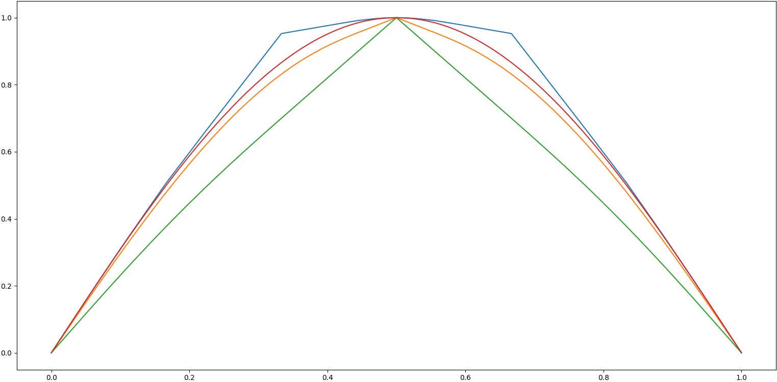
Figure 1. Mather’s $\beta$-function for several convex domains. The red curve corresponds to a disc, the orange to an ellipse of eccentricity $e=0.4$, the green to an ellipse with eccentricity $e=0.9$, and the blue to a curve of constant width.

The length spectrum of $\Omega$ is the collection of all lengths of periodic billiard orbits together with integer multiples of the boundary length (corresponding to gliding orbits). For each $p$, the length spectrum has a finer filtration

$$\text{LSP}(\Omega)=\bigcup_{\begin{subarray}{c}p,q\in\mathbb{N},\\ p/q\leq 1/2\end{subarray}}\text{LSP}_{p,q}(\Omega),$$

where, denoting by $rt(\gamma)=(p,q)$ to be the winding number and the period of a periodic orbit,

$$\text{LSP}_{p,q}(\Omega)=\bigcup_{\gamma\,\text{periodic}}\{\text{length}(\gamma):rt(\gamma)=(p,q)\}.$$

Marvizi and Melrose prove in [MM82] that for each $p\geq 1$, the length spectrum breaks up into little clusters $[t_{p,q},T_{p,q}]$, where

$$t_{p,q}= \inf_{rt(\gamma)=(p,q)}\text{length}(\gamma),$$

$$T_{p,q}= \sup_{rt(\gamma)=(p,q)}\text{length}(\gamma),$$

and $T_{p,q}-t_{p,q}=O_{p}(q^{-\infty})$. For a residual set of boundaries, the length spectrum is simple. For an ellipse, $t_{p,q}=T_{p,q}$ for all $0<p/q<1/2$, corresponding to the one parameter families of orbits tangent to confocal conic sections. In fact, this is true whenever there is a rational caustic of rotation number $p/q$. Marvizi and Melrose go further to show that

(10) $$T_{p,q}\sim p\ell+\sum_{k=1}^{\infty}c_{p,k}q^{-2k},$$

for a sequence of marked length spectral invariants $c_{p,k}$. I follows immediately that the Taylor coefficients of Mather’s $\beta$ function are given by

$$\beta^{2k+1}(0)= \frac{(2k+1)!}{p^{2k+1}}c_{p,k},$$

$$\beta_{2k}= 0.$$

Generically, the wave trace is singular at $\{t_{p,q},T_{p,q}\}$ (the noncoincidence condition in [MM82]) and hence the $c_{p,k}$’s also constitute Laplace spectral invariants ([MM82]). To ensure we have precise control over which orbits end up contributing to the wave trace in our main theorem, we need the following proposition, which states that orbits of a fixed perimeter cannot have arbitrarily large winding number.

Proposition 3.4 ([Kov21b].).

Given any ellipse $\Omega_{0}=\mathcal{E}_{e}$ and $L>0$, there exists a $p_{0}>0$, such that for all $C^{\infty}$ small deformations $\Omega$ and for every $p\geq p_{0}$ and $p/q\leq 1/2$, the minimal length $t_{p,q}$ is strictly greater than $L$.

3.4. Elliptical billiards

Ellipses have special dynamical properties and are conjectured by Birkhoff to be the only (even locally) integrable billiard tables; local integrability here means there is a some neighborhood of phase space which is foliated by caustics. In proving Theorem 1.1, we need to understand how the billiard map behaves under deformation of an ellipse. Let

$$\mathcal{E}_{e}=\{(x,y)\in\mathbb{R}^{2}:x^{2}+\frac{y^{2}}{1-e^{2}}=1\}$$

denote an ellipse which is normalized to have semimajor axis length $1$ and eccentricity $e$. The phase space for the billiard map is the cylinder $\mathcal{E}_{e}\times[-1,1].$ It turns out that all confocal conic sections are caustics for the billiard map on the ellipse. Projecting them onto invariant curves in $B^{*}(\mathcal{E}_{e})$, we can divide the phase space into two regions (see Figure 2). Near the boundary, we have graphs of functions in the $x$ variable which correspond to confocal ellipses; we call these elliptic caustics, even though the corresponding orbits are degenerate. Further from the boundary are billiard orbits which pass between the focal points and are tangent to confocal hyperbolae; we call these hyperbolic caustics. The corresponding invariant circles in phase space (the “eyes”) are homotopic to a point (the “pupil”) on the cylinder. The separatrix between elliptic and hyperbolic invariant curves corresponds to homoclinic orbits which pass through the focal points. For the orbits in the “eyes”, the rotation number, as we defined it before, is always equal to $1/2$. To obtain a more meaningful quantity, we introduce the following:

Definition 3.5.

Let $\gamma$ be an orbit which is tangent to confocal hyperbolae in the ellipse $\mathcal{E}_{e}$ with rotation number $1/2$. We define the libration number of $\gamma$ to be its rotation number when considered as a diffeomorphism of its corresponding invariant circle in phase space.

As mentioned before, all orbits in $\mathcal{E}_{e}$ are degenerate with the exception of the two bouncing ball orbits along the axes of symmetry. The period two orbit along the major axis consists of hyperbolic points on the separatrix, while the bouncing ball along the minor axis is elliptic (the “pupils” of the “eyes”).

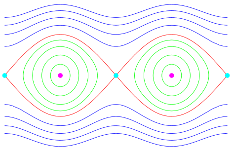
Figure 2. Phase space for billiards on the ellipse. The horizontal axis corresponds to the arclength coordinate along $\partial\Omega$ while the vertical axis corresponds to the dual fiber variable $\sigma=\cos\varphi$. The phase space is symmetric about the midline, corresponding to time reversal of orbits. The blue curves come from “rotations” tangent to confocal ellipses. The green curves are “librations,” corresponding to orbits which pass between the focal points and are tangent to confocal hyperbolae. These two families are separated by the red separatrix, with the three cyan colored dots corresponding to orbits which pass through the focal points, including the bouncing ball along the semimajor axis. The magenta pupils at the center of the “eyes” correspond to the period $2$ bouncing ball orbit along the semiminor axis.

Elliptical polar coordinates $(\varphi,\mu)$ on $\mathbb{R}^{2}$ turn out to be convenient for describing the billiard map. They are given by the coordinate transformation

$$x=-e\cosh\mu\sin\varphi,\qquad y=e\sinh\mu\cos\varphi,$$

where $\{(\pm\pi/2,0)\}$ are focal points for all corresponding coordinate level sets $\mu=\text{const.}$ (confocal ellipses) and $\varphi=\text{const.}$ (confocal hyperbolae). In this case, $\mathcal{E}_{e}$ is parametrized by

$$(-\sin\varphi,\sqrt{1-e^{2}}\cos\varphi).$$

Confocal conic sections are given by

(11) $$\mathcal{E}_{e,\lambda}=\{(x,y)\in\mathbb{R}^{2}:\frac{x^{2}}{1-\lambda^{2}}+\frac{y^{2}}{1-e^{2}-\lambda^{2}}=1\}.$$

For $0\leq\lambda^{2}<1-e^{2}$, the corresponding curves are confocal ellipses while for $1-e^{2}<\lambda^{2}<1$, they are confocal hyperbolae. We also define the incomplete elliptic integrals of the first and second type respectively by

$$F(\varphi,k)=\int_{0}^{\varphi}\frac{d\psi}{\sqrt{1-k^{2}\sin^{2}\psi}},\;\;\;E(\varphi,k)=\int_{0}^{\varphi}\sqrt{1-k^{2}\sin^{2}\psi}d\psi,$$

for $-1<k<1$. Their complete versions are defined by

$$K(k)=F(\pi/2,k),\;\;\;E(k)=E(\pi/2,k).$$

The inverse of an incomplete elliptic integral of the first kind is called the Jacobi amplitude $\text{am}(\eta,k)$:

$$F(\text{am}(\eta,k),k)=\eta.$$

For a confocal conic section $\mathcal{E}_{e,\lambda}$, we set the parameter $k$ in the elliptic integrals above to be the eccentricity of the caustic:

$$k= \frac{e}{\sqrt{1-\lambda^{2}}}.$$

Particularly, $0<k<1$ for elliptic conics and $k>1$ for hyperbolic ones.

Definition 3.6.

Local action angle coordinates for the ellipse $\mathcal{E}_{e}$, on an invariant curve of an elliptic caustic $\mathcal{E}_{e,\lambda}$ are given by $(\eta,I)$, where the angle variable is defined implicitly in terms of the elliptic coordinate $\varphi$ by

$$\varphi=\text{am}\left(\frac{2K(k)}{\pi}\eta,k\right),$$

The action variable $I$ is defined to be the symplectic dual of $\varphi$ and depends on the parameter $\lambda$ corresponding to a confocal conic section in (11), to which a given orbit will be tangent. In these coordinates, the billiard map is given by

$$B(\eta,I)=(\eta+\omega(I),I).$$

We denote by $\Psi_{\text{ell}}$ the corresponding coordinate transformation, so that $\varphi=\pi_{1}\Psi_{\text{ell}}(\eta,I)$, with $\pi_{1}$ being the projection onto the first coordinate.

Definition 3.7.

Local action angle coordinates for the ellipse $\mathcal{E}_{e}$, on an invariant curve of a hyperbolic caustic $\mathcal{E}_{e,\lambda}$ are given by $(\eta,\tilde{\omega}(I))$, where the angle variable is again defined implicitly in terms of the elliptic coordinate $\varphi$ by

$$\varphi=\text{am}\left(\frac{2\tilde{K}(k)}{\pi}\eta,k\right)\mod\pi\mathbb{Z},$$

where $\widetilde{K}\left(k\right)=F\left(\arcsin k^{-1},k\right)$. We again define $I$ to be the symplectic dual coordinate. In these coordinates, the billiard map is given by

$$B(\eta,I)=(\eta+\tilde{\omega}(I),I),$$

where $\tilde{\omega}$ is the libration number. We continue to denote by $\Psi_{\text{hyp.}}$ the corresponding coordinate transformation, so that $\varphi=\pi_{1}\Psi_{\text{hyp.}}(\eta,I)$, with $\pi_{1}$ being the projection onto the first coordinate.

Whenever it is clear from context, we will abbreviate the coordinate transformations $\Psi_{\text{ell.}/\text{hyp.}}$ to $\Psi$.

Remark 3.8.

The reason for computing residues modulo $\pi\mathbb{Z}$ as opposed to $2\pi\mathbb{Z}$ is the presence of two “eyes” in figure 2, with $\eta$ defined separately in each. The billiard map $B$ maps one eye into the other. Note also that by an abuse of notation, we continue to write $F$ and am even when $k>1$.

We now parametrize the reflection points of a periodic orbit associated to an elliptic (resp. hyperbolic) caustic of eccentricity $k$. For an elliptic caustic, the corresponding elliptic coordinates of the reflection points are given by

(12) $$\varphi(s_{i})=\text{am}\left(4K(k)\left(\frac{\eta_{0}}{2\pi}+(i-1)\omega\right),k\right),$$

where $\eta_{0}$ parametrizes the starting point. For a hyperbolic caustic, the situation is more complicated. We have:

(13) $$\varphi(s_{i})=\pi i+\text{am}\left(4\tilde{K}\left(k\right)\left(\frac{\eta_{0}}{2\pi}+(i-1)\tilde{\omega}\right),k\right),$$

where $\tilde{\omega}$ is the libration number defined above. Note that $\arcsin k^{-1}$ is the supremum of arguments of $F$ which give a convergent integral. Usage of the Jacobi amplitude am also needs to be justified. When $k>1$, one can see that $\text{am}\left(\eta,k\right)=\varphi$ is well defined when $\eta\in[-\tilde{K}(k),\tilde{K}(k)]$ and $\varphi\in[-\arcsin k^{-1},\arcsin k^{-1}]$. This allows us to analytically continue the Jacobi amplitude by

$$\text{am}\left(\eta+2\tilde{K}\left(k\right),k\right)=-\text{am}\left(\eta,k\right),\qquad\eta\in\mathbb{R}.$$

We see that in this case, $\varphi$ is restricted to $\left[-\arcsin k^{-1},\arcsin k^{-1}\right]$, together with the shift of this interval by $\pi$. This is to be expected, as all the reflections of the billiard trajectory occur on one side of the hyperbolic caustic.

There are other caustic parameters which are related to $k$ and are connected to billiard dynamics inside the ellipse. Particularly, we have an amplitude which we denote by $\varphi_{0}$, defined by

$$\varphi_{0}= \arcsin\left(\frac{\lambda}{\sqrt{1-e^{2}}}\right),$$

$$\varphi_{0}= \arcsin\left(\frac{\sqrt{1-e^{2}}}{\lambda}\right),$$

for elliptic and hyperbolic caustics respectively.

Remarkably, the rotation number of an elliptic caustic or the libration number of a hyperbolic one can be expressed in terms of these parameters:

$$\omega=\frac{F(\varphi_{0},k)}{2K(k)},\;\;\;\tilde{\omega}=\frac{F(\varphi_{0},k^{-1})}{2K(k^{-1})}.$$

While elliptic caustics with rotation numbers from $0$ to $1/2$ exist for every ellipse, we note that hyperbolic caustics of a given libration number $\tilde{\omega}$ only exist when $e>\cos\pi\tilde{\omega}$. The libration number is strictly monotone in $\lambda$; on the phase portrait shown in Figure 2, the inner curves have larger $\lambda$ and smaller $\tilde{\omega}$.

One is also able to derive formulae for the lengths of periodic orbits in an ellipse. The vertical and horizontal bouncing ball orbits have lengths which are simply four times the lengths of the semi-major and semi-minor axes. According to [Sie97], the lengths of orbits having period greater than two can be expressed in terms of elliptic integrals. For the ellipse $\mathcal{E}_{e}$, orbits tangent to an elliptic caustic $\mathcal{E}_{e,\lambda}$ have lengths given by

(14) $$L_{p,q}=2q\sin\varphi_{0}-\frac{2eq}{k}E(\varphi_{0},k)+\frac{4ep}{k}\mathcal{E}(k).$$

In particular, this gives an expansion of Mather’s beta function near $\omega=0$ and also shows directly that it is smooth, corroborating the remarks made earlier about integrability. Between the focal points, orbits which are tangent to a hyperbolic caustic have lengths given by

(15) $$L_{\tilde{p},q}=2q\sin\varphi_{0}-2eqE(\varphi_{0},k^{-1})+4e\tilde{p}\mathcal{E}(k^{-1}).$$

3.5. Balian-Bloch-Zelditch invariants for nearly-elliptical domains

In [KKV24], the authors derived a formula for the regularized resolvent trace with coefficients called Balian-Bloch-Zelditch (BBZ) wave invariants, which are algebraically equivalent to the full quantum Birkhoff normal form (wave trace invariants). The main theorem in [KKV24] applies to nearly degenerate periodic orbits and gives leading order asymptotics (in the deformation parameter) of the BBZ invariants. We now specialize to the case of $\Omega$ being a deformation of an ellipse. Degenerate orbits which are tangent to a confocal conic section become nearly degenerate after the deformation. As a preliminary step, we recall some notation from [KKV24] and discuss complex phases associated to the Hessian of the length functional.

Proposition 3.9.

Let $\Omega_{0}=\mathcal{E}_{e}$ be an ellipse and $\gamma$ a $q$-periodic orbit which is tangent to an elliptic caustic. Then the Hessian $\partial^{2}\mathcal{L}(S_{\gamma})$ has zero as a simple eigenvalue together with $q-1$ strictly negative ones. Moreover, all entries of the zero eigenvector share a common sign.

Proof.

Denote the elliptic caustic by $\mathcal{E}_{e,\lambda}$. Since it is a caustic, all periodic orbits of type $(p,q)$ share the same length. These orbits realize the maximum of the length functional on $(p,q)$ configurations and hence $\partial\gamma$ is a local maximum for $\mathcal{L}$. This implies that $\partial^{2}\mathcal{L}(S_{\gamma})$ cannot have any positive eigenvalues. We also know that $\gamma$ is degenerate, so the Hessian has nontrivial kernel, corresponding to rotation along a caustic. It remains to show that zero is a simple eigenvalue or alternatively, that the Poincaré map $P_{\gamma}$ is not the identity. We claim that the iterates of $\frac{\partial}{\partial\sigma}$ under $dB^{i}$ have a negative $\frac{\partial}{\partial s}$ component ($\partial s^{\prime}/\partial\sigma<0$) and are thus twisted to the left. On the one hand, these iterates lie on one side of an invariant curve which contains $\gamma$, so the extent to which they can rotate counterclockwise is limited. On the other hand, the twist property prohibits them from rotating clockwise back to the vertical direction. Hence, the Poincaré map is not an identity which concludes the proof. ∎

Lastly, we introduce the adjugate matrix $M:=\text{adj}(\partial^{2}\mathcal{L})$ of the Hessian in $\Omega_{0}$, which was featured in [KKV24]. Its entries are complementary minors of $\partial^{2}\mathcal{L}(\gamma)$, evaluated at boundary points of an ellipse. As shown in [KKV24], $M$ is a real symmetric matrix of rank $1$. Thus, the entries of $M$ are given by

$$M_{\alpha,\beta}=\pm h_{\alpha}h_{\beta},$$

for some $h\in\mathbb{R}^{q}$. As noted in [KKV24], if $\partial^{2}\mathcal{L}$ has a one dimensional kernel, then $h$ is an eigenvector along this direction. In particular, when $\gamma$ is an orbit tangent to an elliptic caustic, all of the $h_{i}$ can be chosen to be positive by Proposition 3.9. We can now state the main result of [KKV24] adapted to ellipses:

Theorem 3.10.

Let $\Omega_{0}=\mathcal{E}_{e}$ be an ellipse and $\gamma$ be a billiard orbit of period $q$, tangent to an elliptic caustic. Assume that $\left\{\Omega_{\varepsilon}\right\}$, $\varepsilon\in[0,\varepsilon_{0}]$ is a smooth family of deformations which fixes the reflection points of $\gamma$. Assume further that the deformation makes $\gamma$ non-degenerate for $\varepsilon>0$, with $|\det\partial^{2}\mathcal{L}|\sim c_{\gamma}\varepsilon$ for some $c_{\gamma}>0$. Then, for $\varepsilon>0$, the $j$-th Balian-Bloch invariant associated to $\gamma$ from (3) has the form

(16) $$\begin{split}B_{j,\gamma}=&\frac{e^{-\frac{i\pi q}{4}}}{q}L_{\gamma}\left(\sum_{i_{1},i_{2},i_{3}=1}^{q}h_{i_{1}}h_{i_{2}}h_{i_{3}}\partial_{i_{1},i_{2},i_{3}}^{3}\mathcal{L}\right)^{2j}(c_{\gamma}\varepsilon)^{-3j}\\ &\times\prod_{l=1}^{q}\frac{\cos\vartheta_{l}}{|x(s_{l})-x(s_{l+1})|}\frac{(\pm i)^{j}}{w(j)}+\mathcal{R}_{j},\end{split}$$

where

• $w(j)=\sum_{\mathcal{G}}\frac{1}{w(\mathcal{G})}>0$ is a sum is over all $3$-regular graphs on $2j$ vertices, with $w(\mathcal{G})$ being the order of the automorphism group of a graph $\mathcal{G}$. In particular, it is independent of both the domain and the orbit. $w(0)=1$.

• The signs $\pm$ are given by $+$ if in the deformed domain $\gamma$ becomes elliptic and $-$ if it becomes hyperbolic.

• $\mathcal{R}_{j}=\mathcal{R}(\gamma,\varepsilon,j,\kappa,\kappa^{(1)},\ldots,\kappa^{(2j)})$, with $\kappa^{(n)}$ being the $n$-th derivative of curvature of $\Omega$ at the reflection points, is a remainder which satisfies:

  • $\varepsilon^{3j-1}\mathcal{R}_{j}$ is smooth in all parameters down to $\varepsilon=0$. Particularly, it is bounded from above whenever the deformation parameters remain bounded and is locally uniformly continuous in them.

  • $\mathcal{R}_{0}=0$.

The prefactor $\mathcal{D}_{\gamma}$ is given by

(17) $$\mathcal{D}_{\gamma}(k)=\frac{e^{ikL_{\gamma}}e^{\frac{i\pi\text{sgn \,}\partial^{2}\mathcal{L}(S_{\gamma})}{4}}}{\sqrt{|\det\partial^{2}\mathcal{L}(S_{\gamma})|}}.$$

Theorem 3.10 gives a formula for the BBZ wave trace invariants associated to a single periodic orbit $\gamma$ of length $L$, traversed in the positive direction. It is essentially an expansion of the regularized resolvent trace ([Zel09]). For a general convex domain, if $L$ is isolated in the length spectrum and all orbits of length $L$ are nondegenerate, the resolvent trace is a sum of contributions of all such orbits. In fact, each such orbit is invariant under both cyclic permutation of the reflection points as well as time reversal, so the trace invariants must be summed over all orbits together with their symmetries. As it does not appear explicitly elsewhere in the literature for billiards, we now show that all symmetries of a periodic orbit generate the same wave trace invariants.

Theorem 3.11.

Let $\Omega$ be any smooth, strictly convex, planar domain and denote by $\gamma$ a nondegenerate $q$-periodic orbit which has no orthogonal angles of reflection. For any $g\in D_{2q}$, the dihedral group on $q$ vertices, define $g\gamma$ to be the $q$-periodic orbit obtained by applying $g$ to the points of reflection $\partial\gamma$. Then $B_{j,g\gamma}=B_{j,\gamma}$ for all $j\in\mathbb{N}$.

Proof.

Corollary 4.12 in [KKV24] shows that

(18) $$\mathcal{D}_{\gamma}(\lambda)\sum_{j=0}^{\infty}B_{j,\gamma}\lambda^{-j}\sim^{*}\sum_{\begin{subarray}{c}1\leq M<\infty\\ \sigma:\mathbb{Z}_{M}\to\{0,1\}\end{subarray}}\frac{e^{-M\pi i/4}}{M}\int_{{\partial\Omega}_{S}^{M}}e^{i\lambda\mathcal{L}(S)}a_{0}^{\sigma}(\lambda,S)dS,$$

where $a_{0}^{\sigma}\in S_{\varrho}^{\frac{M}{2}}(\partial\Omega^{M})$ is a semiclassical symbol which is compactly supported, locally near $\mathcal{L}^{-1}(L)\subset\partial\Omega^{M}$. The notation $\sim^{*}$ indicates, as in [KKV24], that the above is not a true asymptotic expansion but rather, provides an effective algorithm for computing the invariants $B_{\gamma,j}$. The critical points of the phase function occur precisely at the arclength coordinates of $M$-fold billiard orbits of length $L$, including their time reversals and cyclic permutations. The time reversal of an orbit $(x_{1},x_{2},\cdots,x_{q})$ is simply $(x_{q},x_{q-1},\cdots,x_{1})$. The corresponding arclength coordinates are similarly reversed, which corresponds to a change of variables in which one simply permutes the coordinates. The symbol $a_{0}^{\sigma}$ is given in [KKV24] by

$$a_{0}^{\sigma}(k+i\tau,S)=\hat{\rho}(\mathcal{L}(S))\left(\mathcal{L}(S)A_{\sigma}(k+i\tau,S)-\frac{1}{i}\frac{\partial}{\partial k}A_{\sigma}(k+i\tau,S)\right),$$

which belongs to the class $S_{\varrho}^{\frac{M}{2}}(\partial\Omega^{M})$, where $A_{\sigma}(k+i\tau,S)$ is

$$(k+i\tau)^{M/2}\prod_{i=1}^{M}\chi_{i}(k+i\tau,S)\frac{\cos\vartheta_{i}}{|x(s_{i})-x(s_{i+1})|^{1/2}}a_{1}((k+i\tau)|x(s_{i})-x(s_{i+1})|).$$

It is clear that both $\mathcal{L}$ and $a_{0}^{\sigma}$ are invariant under the permutations $s_{i}\mapsto s_{i+j}$ and $s_{i}\mapsto s_{M-i}$. When expanding 18 via the method of stationary phase, the Jacobian has determinant of magnitude one and the measure $dS$ is unoriented, so permutation of the coordinates leaves the integral unchanged. ∎

In light of this, we multiply the leading order term of Theorem 3.10 by $2q$ when summing over all geometrically distinct orbits.

Remark 3.12.

If an orbit has orthogonal reflections at some point, the incident and reflected rays coincide, which reduces the dimension of the configuration. In this case, the symmetry group is also reduced.

We also remark that the third derivative component in (16) is zero for ellipses, since there is a caustic.

Lemma 3.13.

If $\gamma$ is an orbit around an elliptic caustic in $\Omega_{0}=\mathcal{E}_{e}$, we have

(19) $$\partial_{deg}^{3}\mathcal{L}:=\sum_{i_{1},i_{2},i_{3}=1}^{q}h_{i_{1}}h_{i_{2}}h_{i_{3}}\partial_{i_{1},i_{2},i_{3}}^{3}\mathcal{L}=0.$$

Proof.

The expression (19) is the third derivative of $\mathcal{L}$ along the degenerate direction $(h_{1},h_{2},\ldots,h_{q})$. Let $S(\tau)=(s_{1}+\tau h_{1},\ldots,s_{q}+\tau h_{q})$ be a configuration along this subspace. Since $h$ is tangent to the curve of caustic orbit configurations, there exists an orbit $\gamma_{\tau}$ along the caustic with $S_{\gamma_{\tau}}$ being $O(\tau^{2})$ close to $S(\tau)$. We know that $\mathcal{L}_{\Omega_{0}}(S_{\gamma_{\tau}})=L$ and that it is a critical point. Hence,

$$\mathcal{L}_{\Omega_{0}}(S(\tau))=L+\partial\mathcal{L}_{\Omega_{0}}(S_{\gamma_{\tau}})\cdot O(\tau^{2})+O(\tau^{4})=L+O(\tau^{4}).$$

In particular, there is no $\tau^{3}$ term, so the third derivative is $0$. ∎

4. Conjugate Maslov indices

In this section, we find conditions on the Maslov indices of periodic orbits which facilitate cancellations in the wave trace. It is clear that the contribution of just one orbit to the BBZ expansion would be insufficient to make the wave trace smooth at any given length. Indeed, the Poisson relation is an equality whenever the length spectrum is simple, which is a residual property (in the sense of Baire Category Theorem). Instead, multiple orbits of the same length are required to create a cancellation; complex phases arising from Maslov factors together with the corresponding magnitudes $|B_{\gamma,j}|$ of the BBZ wave invariants must align perfectly. Consider the possible phases of $\mathcal{D}_{\gamma}B_{j,\gamma}$ appearing in (4). We will focus on the leading order term in the expansion of $B_{\gamma,j}$, since the error terms $\mathcal{R}_{j}$ are both extremely complicated and relatively small in the deformation parameter. Since the $B_{\gamma,j}$s are complex valued themselves, arranging that they sum to zero does not reduce to a one dimensional problem. The oscillatory part $e^{ikL_{\gamma}}$ in the symplectic prefactor depends on $k$, but appears in the contribution of every orbit, so it can factored out and ignored while keeping track of the phases of individual $B_{\gamma,j}$s.

Without the oscillatory factor $e^{ikL_{\gamma}}$ and the error term $\mathcal{R}_{j}$, $\mathcal{D}_{\gamma}B_{j,\gamma}$ shares its phase with

(20) $$e^{\frac{i\pi\text{sgn \,}\partial^{2}\mathcal{L}(S_{\gamma})}{4}}e^{-\frac{i\pi q}{4}}(\pm i)^{j}.$$

In the unperturbed ellipse $\Omega_{0}=\mathcal{E}_{e}$, if $\gamma$ is tangent to an elliptic caustic and becomes hyperbolic after deformation $\Omega_{\varepsilon}$, then the signature of the Hessian changes to $-q$ and (20) reduces to

$$i^{-q-j}.$$

Alternatively, if the perturbed orbit becomes elliptic, (20) becomes

$$i^{1-q+j}.$$

In total, $4$ phases are possible: $1$, $i$, $-1$ and $-i$. If $\mathcal{D}_{\gamma}(B_{j,\gamma}-\mathcal{R}_{j})$ share the same phase for all $j$, so would their sum and there could be no chance for cancellations. One can try to resolve this issue by having $2$ different phases (say $1$ and $-1$), that will counteract one another. However, the error terms may not be real valued. Hence, we need to choose orbits which realize all $4$ possible phases.

The leading order term of phase $+1$ will be approximately canceled by that of phase $-1$ and the leading order term of phase $+i$ will similarly be approximately canceled by that of phase $-i$. Clearly, each of these orbits will introduce additional error terms, but they are comparatively small and we already have orbits with both real and imaginary phases. The upshot is then that we obtain an open map from the parameter space of deformations to $\mathbb{C}$. We will show that the origin is close to its image by perturbing the domain and cancelling leading order terms. To account for the errors, we use a fixed point argument to show that the map from parameter space to $\mathbb{C}$ in fact covers a neighborhood of the origin.

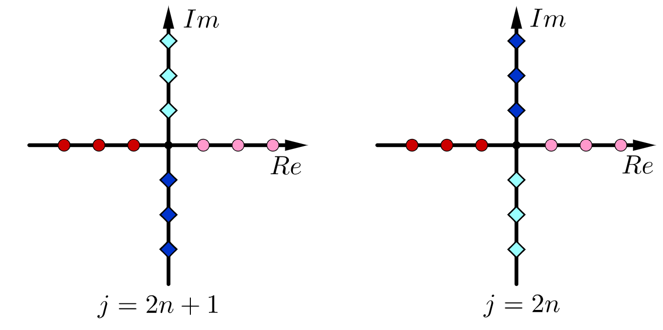
Figure 3. Relative positions of the main contributions on the complex plane for both parities of $j$. There are $4$ types of orbits represented. Lighter colored orbits have rotation number $p/q$, the darker ones – $p^{\prime}/q^{\prime}$. Red and pink orbits (circles) become elliptic while blue and light blue ones (diamonds) become hyperbolic after the deformation.

We now explain how each phase may be realized. Note that if all orbits share the same bounce number $q$, then it would be impossible to create coefficients with all $4$ phases; only $2$ would be possible. Thus, we need at least $2$ periods – call them $q$ and $q^{\prime}$. We consider $4$ families of orbits of varying period and ellipticity/hyperbolicity, as described in the introduction. If we make $q\equiv 0\mod 4$ and $q^{\prime}\equiv 2\mod 4$, we get the following phases for four families:

$$\begin{cases}i^{1+j}&\text{period }q,\,\gamma\text{ elliptic},\\ i^{-j}&\text{period }q,\,\gamma\text{ hyperbolic},\\ i^{-1+j}&\text{period }q^{\prime},\,\gamma\text{ elliptic},\\ i^{2-j}&\text{period }q^{\prime},\,\gamma\text{ hyperbolic}.\end{cases}$$

For a fixed period, we refer to the signatures $\text{sgn \,}\partial^{2}\mathcal{L}(S_{\gamma})$ of elliptic/hyperbolic orbits as conjugate Maslov indices. For any $j\geq 0$, these give all $4$ phases. However, not every ellipse has orbits of the same length but different rotation numbers; we will show that it is indeed possible to do so in the next section (see Theorem 5).

We briefly comment on the number of orbits in each family. Note that in the main term of (16), the only orbit parameters which can be explicitly prescribed under a deformation are $c_{\gamma}\varepsilon$ and

(21) $$\partial_{deg}^{3}\mathcal{L}=\sum_{i_{1},i_{2},i_{3}=1}^{q}h_{i_{1}}h_{i_{2}}h_{i_{3}}\partial_{i_{1},i_{2},i_{3}}^{3}\mathcal{L}.$$

Recall that the expression (21) is zero for $\Omega_{0}=\mathcal{E}_{e}$ (cf. Lemma 19). As we will see later, (21) can be easily prescribed and deformed away from zero. All other parameters in (16) are independent of the deformation; for example $w(j)$ is a combinatorial constant and $\cos\vartheta_{j}$ depends only on the initial orbit. Hence, in contrast to the expansions in [Zel09], there are essentially only $2$ free parameters. To solve the system (4) of $m+1$ equations, we will choose $4$ corresponding families of $m$ orbits each.

5. Length spectral resonances in ellipses

To create arbitrarily high cancellations in the wave trace, we need to find domains with suitably many of orbits of the same length. This section is devoted to finding ellipses for which one has two families of orbits tangent to different caustics, yet having the same length.

Definition 5.1.

We say that $L\in\text{LSP}(\Omega)$ has multiplicity $k$ if there are $k$ distinct closed billiard orbits of length $L$.

Oftentimes in the integrable setting, one has rational caustics which correspond to infinite multiplicity in the length spectrum. In that case, it is useful to generalize the notion of multiplicity:

Definition 5.2.

We say that a domain $\Omega$ has a length spectral resonance if there exist two distinct rational caustics such that all orbits tangent to either caustic have the same length.

We now find suitable ellipses with length spectral resonances.

Lemma 5.3.

Denote by $\beta(\omega;e)$ Mather’s $\beta$ function associated to an ellipse $\mathcal{E}_{e}$ of eccentricity $e$ (cf. Section 3). Then, the ratio

$$\mathcal{R}(\omega_{1},\omega_{2};e)=\frac{\beta(\omega_{1};e)}{\beta(\omega_{2};e)}$$

is analytic in $(\omega_{1},\omega_{2},e)\in(0,1/2)^{2}\times(0,1)$ and nonconstant in $e$.

Proof.

Formulae 14 and 15 give the lengths of periodic orbits in terms of $p,q,k$ and the eccentricity $e$. Dividing by $-q$, we see that

$$\begin{split}\beta\left(\omega\right)=&2\sin\varphi_{0}-2eE\left(\varphi_{0},k\right)+\frac{4e\omega}{k}\mathcal{E}(k)\qquad\text{elliptic caustics},\\ \beta\left(\widetilde{\omega}\right)=&2\sin\varphi_{0}-2eE\left(\varphi_{0},k^{-1}\right)+4e\widetilde{\omega}\mathcal{E}(k^{-1})\qquad\text{hyperbolic caustics}.\end{split}$$

The definitions of $k=k(\lambda;e)$ and $\varphi_{0}=\varphi_{0}(\lambda;e)$ clearly imply analyticity in both $\lambda$ and $e$. The dependence of $\lambda$ on $e$ and $\omega$ is also clearly analytic, from which the first claim follows.

For a circle (eccentricity $e=0$), we have

$$\beta_{0}\left(\frac{p}{q}\right)=2\sin\left(\frac{p\pi}{q}\right),$$

while for a line segment (eccentricity $e=1$), we have

$$\lim_{e\to 1}\beta\left(\frac{p}{q}\right)=2\frac{p}{q}.$$

Consequently, the ratio function for the circle is given by

$$R(\omega_{1},\omega_{2};e)=\frac{\sin\left(\pi\omega_{1}\right)}{\sin\left(\pi\omega_{2}\right)},$$

and for the segment by

$$R(\omega_{1},\omega_{2};e)=\frac{\omega_{1}}{\omega_{2}}.$$

Hence the ratio function $\mathcal{R}(\omega_{1},\omega_{2};e)$ is real analytic and nonconstant in $e$. ∎

Lemma 5.4.

There are at most finitely many points $E=\{e_{i}\}_{i=1}^{n}\cup\{1\}$ such that for each $\varepsilon>0$ and $\text{dist}(e,E)>\varepsilon$, there exist constants $c(\varepsilon),\delta(\varepsilon)>0$ with the property that whenever $\omega_{1},\omega_{2}\leq\delta$,

$$\left|\frac{\partial}{\partial e}\mathcal{R}(\omega_{1},\omega_{2};e)\right|\geq c(\varepsilon)\left|\omega_{2}\omega_{1}^{3}-\omega_{1}\omega_{2}^{3}\right|,$$

Proof.

Note that the expansion of Mather’s $\beta$ function converges uniformly for $e\in[0,1-\varepsilon]$:

$$\beta(\omega_{i};e)\sim\beta_{1}(e)\omega_{i}+\beta_{3}(e)\omega_{i}^{3}+O_{e}(\omega_{i}^{5}).$$

From [Sor15], we know that

(22) $$\begin{split}\beta_{1}(e)=&\ell=|\partial\Omega_{e}|,\\ \beta_{3}(e)=&-\frac{1}{4}\left(\int_{0}^{\ell}\kappa^{2/3}(s)ds\right)^{3},\end{split}$$

$\kappa$ being the curvature of $\mathcal{E}_{e}$ in arclength coordinates. The remainder is again uniform in $e\in[0,1-\varepsilon]$. Noting that $\omega_{2}\lesssim_{e}|\beta(\omega_{2};e)|=O_{e}(1)$ uniformly, we have

(23) $$\frac{\partial}{\partial e}\mathcal{R}(\omega_{1},\omega_{2};e)=\frac{\left(\beta_{1}\frac{\partial\beta_{3}}{\partial e}-\beta_{3}\frac{\partial\beta_{1}}{\partial e}\right)\left(\omega_{2}\omega_{1}^{3}-\omega_{1}\omega_{2}^{3}\right)+r(\omega_{1},\omega_{2};e)}{\beta(\omega_{2};e)^{2}},$$

where $r=O_{e}(\omega_{1}^{5}+\omega_{2}^{5})$ is another remainder. To compute $\beta_{i}$ for the ellipse, it is simpler to use the formulae 22, rather than differentiating 14 and 15. We parametrize the ellipse $\mathcal{E}_{e}$ by $(-\sin t,(1-e^{2})^{1/2}\cos t)$ so that

$$\begin{split}\beta_{1}(e)=&\int_{0}^{2\pi}(1-e^{2}\sin^{2}t)^{1/2}dt,\\ \beta_{3}(e)=&-\frac{1}{4}\left(\int_{0}^{2\pi}\left(1-e^{2}\sin^{2}t\right)^{-1/2}dt\right)^{3}.\end{split}$$

Differentiating, we find that

$$\frac{\partial\beta_{1}}{\partial e}= -\int_{0}^{2\pi}\frac{e\sin^{2}t}{(1-e^{2}\sin^{2}t)^{1/2}}dt,$$

$$\frac{\partial\beta_{3}}{\partial e}= \frac{3}{4}(1-e^{2})\left(\int_{0}^{2\pi}\left(1-e^{2}\sin^{2}t\right)^{-1/2}dt\right)^{2}\int_{0}^{2\pi}\frac{e\sin^{2}t}{(1-e^{2}\sin^{2}t)^{3/2}}dt$$

$$+\frac{e}{2}\left(\int_{0}^{2\pi}\left(1-e^{2}\sin^{2}t\right)^{-1/2}dt\right)^{3}.$$

Denote by $I_{p}$ the integrals

$$I_{p}=\int_{0}^{2\pi}\frac{\sin^{2}t}{(1-e^{2}\sin^{2}t)^{p/2}},$$

for $p=1,2$ and by $I_{0}$, the integral

$$I_{0}=\int_{0}^{2\pi}(1-e^{2}\sin^{2}t)^{-1/2}=4K(e).$$

We then have

$$\beta_{1}\frac{\partial\beta_{3}}{\partial e}-\beta_{3}\frac{\partial\beta_{1}}{\partial e}=-e\ell I_{0}^{2}\left(\frac{3}{4}I_{3}-\frac{1}{2}I_{0}-\frac{(1-e^{2})}{4\ell}I_{0}I_{1}\right).$$

When $e=0$, corresponding to a circle, $I_{0}=2\pi$ and $I_{1}=I_{3}=\pi$. Hence, for $e$ small, we have

$$\beta_{1}\frac{\partial\beta_{3}}{\partial e}-\beta_{3}\frac{\partial\beta_{1}}{\partial e}\sim 4\pi^{4}e+O(e^{2}).$$

This gives a lower bound on the truncated Taylor series of $\frac{\partial}{\partial e}\mathcal{R}$, which shows in particular that it is nonzero and nonconstant (in $e$). Hence its zeros

$$E=\left\{e:\frac{\partial\mathcal{R}}{\partial e}=0\right\}\cup\{1\}$$

are isolated and of finite multiplicity. Away from an $\varepsilon$ neighborhood of $E$ and $\omega_{i}<\delta(\varepsilon)$, the estimate on $\beta(\omega_{2};e)$ together with 23 implies that

$$\frac{\partial}{\partial e}\mathcal{R}(\omega_{1},\omega_{2};e)\gtrsim_{e}c(\varepsilon)\left(\omega_{2}\omega_{1}^{3}-\omega_{1}\omega_{2}^{3}\right).$$

∎

Theorem 5.5.

There exists a dense set of eccentricities $e$ such that any ellipse of eccentricity $e$ has at least two rational caustics of distinct types $(p,q)$ and $(p^{\prime},q^{\prime})$, with all corresponding orbits having the same length. Moreover, for any $m,n\in\mathbb{Z}$, one can choose such caustics to satisfy $q=q^{\prime}+m\mod n$.

Proof.

Fix $e_{0}\in(0,1)\backslash E$ and suppose $\beta_{e_{0}}(\omega_{1})/\beta_{e_{0}}(\omega_{2})=\tau\in\mathbb{R}\backslash\mathbb{Q}$ for some $\omega_{1},\omega_{2}\in\mathbb{R}\backslash\mathbb{Q}$. We can approximate

$$\tau=\lim_{k\to\infty}\frac{q_{2}(k)}{q_{1}(k)}$$

by a sequence of rationals. For any $\varepsilon>0$ there exists $k_{0}\in\mathbb{N}$ such that for all $k\geq k_{0}$, we have

$$\left|\tau-\frac{q_{2}(k)}{q_{1}(k)}\right|<\varepsilon.$$

As $\tau$ is irrational, each of the sequences $p_{1}(k),p_{2}(k),q_{1}(k),q_{2}(k)$ tends to infinity as $k\to\infty$ and since $\omega_{1}$ and $\omega_{2}$ are irrational, they can individually be approximated by two other sequences

$$\lim_{k\to\infty}\frac{p_{j}(k)}{q_{j}(k)}=\omega_{j},\text{ for }j=1,2.$$

It is also clear that we can choose the residues of $q_{1}(k)$ and $q_{2}(k)$ modulo $n$, since

$$\frac{q_{2}(k)-q_{1}(k)\mod n}{q_{2}(k)}\to 0,$$

as $k\to\infty$. In particular, there exists a $k_{1}\in\mathbb{N}$ such that for all $k\geq k_{1}$ we have

$$\left|\omega_{j}-\frac{p_{j}(k)}{q_{j}(k)}\right|<\varepsilon.$$

Note that

$$\frac{\beta_{e_{0}}\left(\frac{p_{1}(k)}{q_{1}(k)}\right)}{\beta_{e_{0}}\left(\frac{p_{2}(k)}{q_{2}(k)}\right)}$$

approximates $\tau$ arbitrarily well. Choose $k_{2}$ so that for all $k\geq k_{2}$,

$$\left|\frac{\beta_{e_{0}}\left(\frac{p_{1}(k)}{q_{1}(k)}\right)}{\beta_{e_{0}}\left(\frac{p_{2}(k)}{q_{2}(k)}\right)}-\tau\right|<\varepsilon.$$

Since the ratio function

$$R\left(\frac{p_{1}(k)}{q_{1}(k)},\frac{p_{2}(k)}{q_{2}(k)};e\right)=\frac{\beta_{e}\left(\frac{p_{1}(k)}{q_{1}(k)}\right)}{\beta_{e}\left(\frac{p_{2}(k)}{q_{2}(k)}\right)}$$

is nontrivial and analytic as a function of $e$, with a lower bound on its derivative from Lemma 5.4, we can use the quantitative implicit function theorem (see e.g. [Liv]) to see that for some $e_{k}$ close to $e_{0}$, this ratio equals $q_{2}(k)/q_{1}(k)$. In other words, $e_{k}$ solves the length spectral resonance equation

$$q_{1}(k)\cdot\beta_{e_{k}}\left(\frac{p_{1}(k)}{q_{1}(k)}\right)=q_{2}(k)\cdot\beta_{e_{k}}\left(\frac{p_{2}(k)}{q_{2}(k)}\right).$$

Again due to the nontrivial dependence on $e$ and the implicit function theorem, we can choose a sequence $e_{k}$ converging to $e_{0}$ along a sequence of solutions to the length spectral resonance equation. For any $\delta>0$, there is $k_{2}$ such that whenever $k>k_{2}$, the ratio

$$\frac{q_{1}(k)\cdot\beta_{e_{k}}\left(\frac{p_{1}(k)}{q_{1}(k)}\right)}{q_{2}(k)\cdot\beta_{e_{k}}\left(\frac{p_{2}(k)}{q_{2}(k)}\right)}$$

is $\frac{\delta}{2}$ close to $1$. The lemma then follows. ∎

Remark 5.6.

The family of ellipses with length spectral resonances is dense, but nevertheless has measure $0$ and is in fact countable. This follows from the fact that the lengths of all orbits are given by functions (14) and (15) which are analytic in $e$. Since there are only countably many pairs $(p,q)$ or $(\tilde{p},q)$, proving countable resonance between any two given pairs is sufficient. However, those resonances are the zeros of analytic functions and thus are either locally finite or coincide with the domain of definition. The latter case (identity resonance) can be excluded by considering expansions as $e\rightarrow 1$.

6. Destroying stray orbits

6.1. Controllable family of deformations

We begin with an ellipse $\Omega_{0}=\mathcal{E}_{e}$ satisfying the hypotheses of Theorem 5.5; there are one parameter families of type $(p,q)$ and type $(p^{\prime},q^{\prime})$ orbits which are tangent to confocal ellipses and share the same length, $L$. Let $\Omega$ be any $C^{\infty}$-small deformation of $\Omega_{0}$ which preserves a family $\mathcal{F}_{m}$ of $4m$ distinct periodic orbits – $2m$ of type $(p,q)$ and $2m$ of type $(p^{\prime},q^{\prime})$.

Definition 6.1.

Let $\Omega_{0}\mapsto\Omega$ be a deformation of the ellipse as described above. A stray orbit of length $L$ is an orbit in $\Omega$ which has length $L$ and does not belong to the family $\mathcal{F}_{m}$ of $4m$ preserved orbits.

Our aim is to prescribe a deformation which destroys any additional stray orbits of the same length $L$, which will lead to cancellations in Theorem 1.1. They will preserve $4m$ orbits inside of an ellipse, provide needed values of $\det\partial^{2}\mathcal{L}$ and $\partial_{deg}^{3}\mathcal{L}$ and destroy other orbits of length $L$. In Section 7, we will use this family to match the parameters and create cancellations.

Figure 4. An ellipse with $4m$ orbits selected ($m=2$). There are $4$ families of orbits. Lighter colored orbits have rotation number $p/q$ and the darker ones – $p^{\prime}/q^{\prime}$. Red and pink orbits (circles) will become elliptic while blue and light blue ones (diamonds) will become hyperbolic after the deformation.

Definition 6.2.

Let $m>1$ and $\Omega_{0}=\mathcal{E}_{e}$ be an ellipse satisfying the length spectral resonance condition in Theorem 5.5. We introduce the parameters $\bar{\varepsilon}=(\varepsilon_{1},\ldots,\varepsilon_{4m})$ and $\bar{\delta}=(\delta_{1},\ldots,\delta_{4m})$, with $0<\varepsilon_{u}<\varepsilon_{0}$ and $\sqrt{\varepsilon_{u}}<\delta_{u}<\delta_{0}$ for every $u=1,\ldots,4m$ and some fixed $\varepsilon_{0},\delta_{0}>0$. We call a family of deformations $\left\{\Omega_{\bar{\varepsilon},\bar{\delta}}\right\}$ controllable if the following conditions hold:

1. $\Omega_{\bar{\varepsilon},\bar{\delta}}$ is a multiscale normal deformation of $\Omega_{0}$, by which we mean that

   (24) $$\Omega_{\bar{\varepsilon},\bar{\delta}}=\Omega_{0}+\mu_{\bar{\varepsilon},\bar{\delta}}(s)\vec{n}(s).$$

2. There is a family $\mathcal{F}_{m}=\left\{\gamma_{u}\right\}_{u=1}^{4m}$ consisting of $4m$ periodic orbits in $\Omega_{0}$, all of which have the same length and remain fixed in $\Omega_{\bar{\varepsilon},\bar{\delta}}$, i.e. the deformation makes first order contact with $\Omega_{0}$ at the reflection points of each orbit. The first $2m$ are of type $(p,q)$ and are tangent to a caustic $\Gamma$, while the last $2m$ are of type $(p^{\prime},q^{\prime})$ and are tangent to a second caustic $\Gamma^{\prime}$. We denote the collection of their reflection points by $\partial\mathcal{F}_{m}$ and individually by $x_{i}$, $1\leq i\leq 2m(q+q^{\prime})$.

3. In $\Omega_{\bar{\varepsilon},\bar{\delta}}$, the orbits $\gamma_{u}$, for $u=1,\ldots,m$ and $u=2m+1,\ldots,3m$, are hyperbolic while the others are elliptic.

4. For $u=1,\ldots,4m$, we have

   $$|\det\partial^{2}\mathcal{L}(\gamma_{u})|=\varepsilon_{u},\;\;\;\partial_{deg}^{3}\mathcal{L}=\delta_{u}.$$

5. There are no additional stray orbits of length $L$ in $\Omega_{\bar{\varepsilon},\bar{\delta}}$ and $L$ is isolated in the length spectrum.

6. The perimeter of $\Omega_{\bar{\varepsilon},\bar{\delta}}$ is strictly less then that of $\Omega_{0}$.

7. For all $\bar{\varepsilon},\bar{\delta}$, the deformation $\mu_{\bar{\varepsilon},\bar{\delta}}(s)$ remains in a fixed $C^{\infty}$ neighborhood of $0$.

8. There exists a $\xi>0$ such that for each $\gamma_{u}\in\mathcal{F}_{m}$, the perturbation $\mu$ satisfies

   $$\left\|\mu_{\bar{\varepsilon},\bar{\delta}}(s)|_{\left(s_{i}(\gamma_{u})-\xi,s_{i}(\gamma_{u})+\xi\right)}\right\|_{C^{2m+2}}=O(\max(\varepsilon_{u},\delta_{u})),$$

   where $s_{i}(\gamma_{u})$ are the arclength coordinates of reflection points of $\gamma_{u}$.

While Condition $8$ above guarantees that the deformation $\Omega$ will be $\bar{\varepsilon}$-$\bar{\delta}$-close to $\Omega_{0}$ in a neighborhood of the reflection points of selected orbits, no constraints are imposed away from them. In what follows, our deformation $\mu$ will be split into local (near the reflection points) and nonlocal (away from them) zones. If we denote these by $\mu_{1}$ and $\mu_{2}$ respectively, then Condition $8$ asserts that $\|\mu_{1}\|_{C^{2m+2}}\lesssim\max(\|\bar{\varepsilon}\|,\|\bar{\delta}\|)$. We will measure the norm of $\mu=\mu_{1}+\mu_{2}$ by an independent parameter $\iota$, which is allowed to be much greater than $\|\bar{\varepsilon}\|,\|\bar{\delta}\|$; it effectively measures the size of $\mu_{2}$ and need not be $o(1)$ with respect to $\|\bar{\varepsilon}\|,\|\bar{\delta}\|$.

Remark 6.3.

Note that if $\iota\neq o(1)$ with respect to $\|\bar{\varepsilon}\|,\|\bar{\delta}\|$, then the limiting domain of $\Omega_{\bar{\varepsilon},\bar{\delta}}$ as $\bar{\varepsilon},\bar{\delta}\to 0$ will not be an ellipse. If the perturbation is $C^{2}$-small (independently of $\bar{\varepsilon},\bar{\delta}$), then convexity will be preserved.

The remainder of this section will be dedicated to a proof of the following theorem.

Theorem 6.4.

For every $m>1$, there exist controllable families of deformations in any $C^{\infty}$ neighborhood of $\Omega_{0}$.

Remark 6.5.

The proof of Theorem 6.4 is quite technical. With no loss of continuity, the reader may skip ahead directly to Section 7 in order to see how the existence of controllable families implies Theorem 1.1.

The deformation $\mu$ will be divided into two zones. In a neighborhood of the reflection points of preserved orbits $\gamma_{u}\in\mathcal{F}_{m}$, finer control is required: $\mu$ is smaller with respect to the $C^{\infty}$ topology and the Hessian of the length functional $\mathcal{L}$ will be prescribed there. Outside of this neighborhood, there is more freedom to deform the domain but we must eliminate all stray orbits of length $L$. The rationale for such a decomposition into local and nonlocal zones is the dependence of Balian-Bloch-Zelditch wave invariants only on the local geometry of the boundary near reflection points in $\partial\mathcal{F}_{m}$. As above, we will correspondingly decompose the normal deformation into $\mu=\mu_{1}+\mu_{2}$, with $\mu_{1}$ and $\mu_{2}$ supported near the local and nonlocal zones respectively. Moving forward, we will denote by $\partial\mathcal{F}_{m}\subset\partial\Omega^{2m(q+q^{\prime})}$ the collection of all reflection points of the $4m$ selected orbits in $\mathcal{F}_{m}$. The proof of Theorem 6.4 has four main steps.

• Orbit selection. In Definition 6.10, we introduce the notion of a correctly selected family of orbits in the starting ellipse $\mathcal{E}_{e}$. We denote by $\mathcal{F}_{m}$ a family of $4m$ orbits, $2m$ having type $(p,q)$ and $2m$ having type $(p^{\prime},q^{\prime})$. The conditions are combinatorial in nature and ensure that the reflection points of orbits (not necessarily those in $\mathcal{F}_{m}$) are sufficiently disjoint. This makes it possible to deform $\mathcal{E}_{e}$ within a controllable family in Steps $2$ and $3$ below. To show that such families exist, we show in Proposition 6.12 that orbits which are not correctly selected form a union of submanifolds in the configuration space $\mathcal{E}_{e}^{4m}$ which have positive codimension. In particular, “correctly selected” is an open and full measure condition.

• Nonlocal deformation. Having fixed a family $\mathcal{F}_{m}$ of $4m$ correctly selected orbits, the main idea is to make the nonlocal part $\mu_{2}$ of the deformation $\mu$ negative while preserving convexity. This will decrease the perimeter of $\Omega_{0}$ together with the lengths of all possible stray orbits of length $L$ which avoid a neighborhood of $\partial\mathcal{F}_{m}$. The norm of $\mu_{2}$ is measured by an independent parameter $\iota$ and is allowed to be much greater than $\mu_{1}$, unrestricted by the deformation parameters $\bar{\varepsilon}$ and $\bar{\delta}$. Hence, if even one reflection point of a potentially stray orbit falls in the nonlocal zone, its length will shrink to less than $L$, the length at which we localized the wave trace; the negativity of $\mu_{2}$ will dominate whatever influence $\mu_{1}$ has on the length functional $\mathcal{L}$, allowing more freedom with $\mu_{1}$ to prescribe the curvature jet at reflection points of $\mathcal{F}_{m}$. Both $\mu_{1}$ and $\mu_{2}$ will be smooth.

• Local deformation. Without loss of generality, for each $\gamma_{u}\in\mathcal{F}_{m}$, we may select a first (marked) reflection point, which we denote by $x_{u}^{1}$. Define the set of all first reflection points of orbits in $\mathcal{F}_{m}$ to be $\partial\mathcal{F}_{m}^{1}$. In order to simplify the construction of $\mu_{1}$, we localize its support to a neighborhood $\mathcal{F}_{m}^{1}$; the deformation $\mu$ will leave unchanged the boundary of $\Omega_{0}$ near the remaining $2m(q+q^{\prime}-2)$ reflection points. This will also simplify the exclusion of stray orbits which reflect in a neighborhood of $\partial\mathcal{F}_{m}$.

Theorem 6.6.

In $\Omega_{0}=\mathcal{E}_{e}$, there exists a $C_{0}(e)$ such that for any $C\geq C_{0}$ and $\xi>1$, one can select the positions of $4m$ orbits and an arbitrarily $C^{\infty}$-small deformation $\mu_{2}$, which is identically $0$ on a $\xi$-neighborhood of $\mathcal{F}_{m}$, such that the following holds: for every $C^{\infty}$-small $\mu_{1}$ which is supported on a $C\xi$-neighborhood of $\partial\mathcal{F}_{m}^{1}$, the $\mu=\mu_{1}+\mu_{2}$ deformed domain $\Omega$ has no stray orbits of length $L$, provided that $\Omega$ and $\Omega_{0}$ make first order contact ($\mu(s)=\mu^{\prime}(s)=0$) only at $\partial\mathcal{F}_{m}^{1}$ within a $C\xi$-neighborhood of $\partial\mathcal{F}_{m}^{1}$.

We will first construct $\mu_{2}(s)$ and then apply Theorem 6.6 to pick a local deformation $\mu_{1}$ in Section 6.4, which will give the needed $3$-jet at reflection points while simultaneously eliminating stray orbits. Such a pair will give rise to a deformation $\mu$ satisfying the conditions of Definition 6.2.

6.2. Preliminaries

We first tabulate some important properties of stray orbits which will be used throughout this section. Assume that a stray orbit of length $L$ exists and is of type $(p^{\prime\prime},q^{\prime\prime})$. We first bound $p^{\prime\prime}$ and $q^{\prime\prime}$:

Lemma 6.7.

There exist $p_{0}$ and $q_{0}$ such that for every $C^{\infty}$-small perimeter decreasing deformation $\Omega$ of $\Omega_{0}$, the length $L$ cannot be achieved by orbits of type $(p^{\prime\prime},q^{\prime\prime})$ whenever $p^{\prime\prime}>p_{0}$ or $q^{\prime\prime}>q_{0}$.

Proof.

From Proposition 3.9, we know that $p^{\prime\prime}$ is bounded by a fixed $p_{0}$. To bound $q^{\prime\prime}$, we use (10) and Lemma 8.7 in [Kov21b]. Since $p^{\prime\prime}$ is already bounded, all orbits of type $(p,q)$ with sufficiently large $q$ belong to a small neighborhood of $p|\partial\Omega|$. If $L\neq p|\partial\Omega_{0}|$ for some $p$, then $L\neq p|\partial\Omega|$, since $|\partial\Omega|$ and $c_{p,1}$ (the first Marvizi-Melrose invariant, cf. equation (10)) are continuous with respect to $C^{\infty}$ deformations. If $L=p|\partial\Omega|$ for some $p$, we require our deformation to decrease the perimeter of $\Omega_{0}$. In that case, $p|\partial\Omega|<L$ and since $c_{p,1}<0$, the lengths of type $(p,q)$ orbits accumulate at $|\partial\Omega|$ from below. In particular, they do not coincide with $L$. ∎

Throughout the rest of the paper, we will denote the diffeomorphism mapping $\partial\Omega_{0}\to\partial\Omega$ by

$$\Phi_{\mu}(x)=x+\mu_{\bar{\varepsilon},\bar{\delta}}(x)n(x)\in\partial\Omega,$$

and its induced product map by

(25) $$\Phi_{\mu,q}:=\Phi_{\mu}\underbrace{\times\cdots\times}_{q\text{ times}}\Phi_{\mu}:\partial\Omega_{0}^{q}\to\partial\Omega^{q}.$$

By an abuse of notation, we will sometimes write $\Phi_{\mu,q}$ with an argument in either arclength or action angle coordinates, as opposed to Euclidean coordinates on $\mathbb{R}^{2}$.

It follows from Lemma 6.7 that lengths of orbits in $\Omega$ are close to lengths in $\Omega_{0}$:

Proposition 6.8 ([Kov21a]).

Let $L_{p,q}(\Omega)\in\text{LSP}_{p,q}(\Omega)$, where $\Omega$ is a $C^{\infty}$-small normal deformation of the ellipse $\Omega_{0}=\mathcal{E}_{e}$ (Condition 1 in Definition 6.2). Then, there exists $L_{p,q}(\Omega_{0})\in\text{LSP}_{p,q}(\Omega_{0})$, such that:

(26) $$|L_{p,q}(\Omega)-L_{p,q}(\Omega_{0})|=o_{p,q,e}(1),$$

with respect to the $C^{\infty}$ distance on boundary curvatures. Moreover, for every type $(p,q)$ orbit $\gamma^{\prime}$ in $\Omega$, there exists a type $(p,q)$ orbit $\gamma$ in $\Omega_{0}=\mathcal{E}_{e}$ such that $\Phi_{\mu,q}^{-1}(\partial\gamma^{\prime})$ is $o_{p,q,\Omega_{0}}(1)$-close to $\gamma$ with respect to the $C^{\infty}$ topology on $\mu$.

Since $p$ and $q$ are already bounded by Lemma 6.7, the $o_{p,q,\Omega_{0}}(1)$ estimates above can be made uniform. Note also that the type $(p,q)$ part of the length spectrum of an ellipse is finite for $p,q$ bounded. Hence there can be no accumulation at the specified length $L$ and an orbit of length $L$ in $\Omega$ must be close to an orbit of length $L$ in the ellipse.

Thus, any stray orbit in $\Omega$ will be close to some orbit in $\Omega_{0}$ of length $L$. As long as we ensure that the deformation either decreases or increases their lengths, there will be no stray orbits in $\Omega$.

Remark 6.9.

In Definition 6.2, we also required that $L$ be isolated in the length spectrum. Theorem 6.6 does not address this directly. However, if $L$ were an accumulation point in the length spectrum, Lemma would 6.7 imply that the corresponding orbits would have bounded $p$ and $q$. The arclength coordinates of these trajectories would belong to the compact set $\cup_{q\leq q_{0}}\mathbb{T}_{\ell}^{q}$ and hence have a convergent subsequence. By continuity, such a limit point would correspond to a degenerate billiard trajectory of length $L$. As our construction rules out all degenerate trajectories of length $L$, it follows that $L$ must be isolated in the length spectrum.

6.3. Proof of Theorem 6.6

6.3.1. Part 1: orbit selection

We now select the exact positions of our $4m$ fixed periodic orbits in the ellipse $\Omega_{0}=\mathcal{E}_{e}$. Any caustic provides a one parameter family of possible orbits, but there are additional constraints. For example, suppose that some other orbit (not one of the $4m$ fixed ones) of length $L$ in $\Omega_{0}$ has reflection points contained in a subset of $\mathcal{S}$. Since our deformation makes first order contact at $\mathcal{S}$, this stray orbit will persist through any controllable deformation we create. To ensure such problems don’t arise, we introduce the following four requirements for orbit selection.

Definition 6.10.

We call a family $\mathcal{F}_{m}=\left\{\gamma_{u}\right\}$ of $4m$ orbits in $\mathcal{E}_{e}$ correctly selected if the following conditions hold:

1. If $\gamma_{u}$ is selected, then no other orbit $\gamma$ of length $L$ in $\mathcal{E}_{e}$ can have $\partial\gamma\subset\partial\gamma_{u}$.

2. If $\gamma_{u}$ is selected, its reflection points do not lie on the minor axis of an ellipse.

3. If $\gamma_{u}$ and $\gamma_{v}$ are selected, their reflection points are disjoint.

4. If $\gamma_{u}$ and $\gamma_{v}$ are selected, there does not exist any orbit of length $L$ in $\Omega_{0}=\mathcal{E}_{e}$ which shares its reflection points with both $\gamma_{u}$ and $\gamma_{v}$.

Definition 6.11.

Whenever $\partial\gamma\subset\partial\gamma^{\prime}$ for some orbits $\gamma,\gamma^{\prime}$ (the negation of Condition $1$ above), we say that $\gamma^{\prime}$ covers $\gamma$.

Conditions $1$ and $4$ forbid stray orbits with reflection points in $\mathcal{S}$. Condition $3$ allows us to change $\mu_{1}$ independently for each orbit, with no risk of interference from the others. As we shall see, it is harder to prove that bouncing ball orbits along the minor axis do not give rise to stray orbits, so Condition $2$ is useful in the event that the length of the minor axis divides $L$. Note also that Conditions $2$, $3$ and $4$ hold outside of the union of (stratified) submanifolds which have positive codimension in $\partial\Omega^{2m(q+q^{\prime})}$. In particular, they are open and full measure conditions, so they can be easily satisfied. For example, among the one parameter family of orbits tangent to any given caustic, only finitely many other have reflection points on the minor axis. Similarly, after fixing any such chosen orbit, only finitely many others share a common point of reflection.

Note that Conditions $1$ and $4$ in Definition 6.10 pertain to all orbits in $\mathcal{E}_{e}$, not just those in $\mathcal{F}_{m}$. This makes them more difficult to verify than Conditions $2$ and $3$. However, for Condition $4$, we can argue as follows. Consider an orbit $\gamma$ and the collection of all others of length $L$ in $\mathcal{E}_{e}$ (having any rotation number) which share a common point of reflection with $\gamma$. Lemma 6.7 guarantees that there are at most a finite number of possible rotation numbers, so there are only finitely many orbits.

This type of argument unfortunately tells us nothing about Condition $1$. If one rotates an orbit of type $(p,q)$ and length $L$ around a caustic in $\mathcal{E}_{e}$, a priori, there may persist another orbit of length $L$ which remains covered by it. We claim that aside from a finite number of exceptions, this cannot happen.

Proposition 6.12.

There are at most finitely many orbits in the ellipse $\Omega_{0}=\mathcal{E}_{e}$ which violate Condition $1$ in Definition 6.10.

Proof.

The negation of Condition 1 is that for a family of $4m$ orbits of length $L$, there exists an orbit external to $\mathcal{F}_{m}$ which shares a common reflection point with one in $\mathcal{F}_{m}$. Note that by Lemma 6.7, it suffices to prove the lemma for orbits of a fixed type, say type-$(p,q)$. Such an orbit will be tangent to either an elliptic or hyperbolic caustic, pass through the focal points or be a bouncing ball orbit along the minor axis. The only periodic orbits through focal points are bouncing ball orbits along the major axis. It is clear that at most finitely many bouncing ball orbits along either axis can have length $L$.

Assume that some type-$(p,q)$ orbit $\gamma$ fully covers another orbit $\zeta$ of type $(p^{\prime\prime},q^{\prime\prime})$. Denote their corresponding caustics by $\Gamma_{\gamma}$ and $\Gamma_{\zeta}$. Without loss of generality, assume that the first points of $\gamma$ and $\zeta$ coincide and denote their corresponding elliptical polar coordinate by $\varphi_{1}$. The second reflection point of $\partial\zeta$ coincides with the $i+1$-st of $\partial\gamma$ for some $i$, and we denote the corresponding coordinate by $\varphi_{i+1}$.

We now rotate $\gamma$ along $\Gamma_{\gamma}$ by changing $\varphi_{1}$ and ask whether the covering will persist. By formulae (12) and (13), $\varphi_{i+1}$ depends analytically on $\varphi_{1}$. Similarly, the elliptical polar coordinate of the second reflection point of $\zeta$ (call it ${\varphi}_{2}^{\prime\prime}$) depends analytically on $\varphi_{1}$ when rotated simultaneously along $\Gamma_{\zeta}$. Hence, their reflection points coincide on the zero set of a real analytic function – that is, either everywhere on the complex domain or only on a locally finite set.

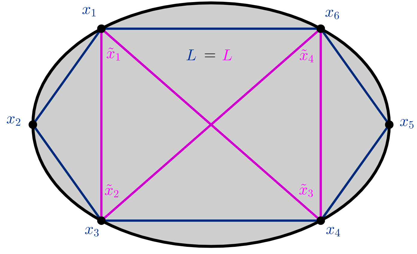
Figure 5. A potential example of an orbit, not satisfying the first selection condition. In this case, the selected orbit (in blue) has $p=1$ and $q=6$, whereas the stray orbit is tangent to a hyperbolic caustic, with $\tilde{p}^{\prime\prime}=1$ and $q^{\prime\prime}=4$. The figure is for illustration purposes only and is not drawn to scale – the actual orbits in this ellipse may have different lengths and/or reflection points.

We focus on a single orbit $\gamma$ which is tangent to an elliptic caustic; in this case, $\varphi_{i+1}$ extends to an analytic function of $\varphi_{1}$ on a complex strip containing the real axis. The same holds for ${\varphi}_{2}^{\prime\prime}$, if $\zeta$ is also tangent to a confocal ellipse. However, if $\zeta$ is tangent to a confocal hyperbola and $x_{1}$ is on the lower side of an ellipse, ${\varphi}_{2}^{\prime\prime}(\varphi_{1})$ is defined only for $\varphi_{1}\in[-\arcsin k^{\prime\prime-1},\arcsin k^{\prime\prime-1}]$, where

$$k^{\prime\prime}=\frac{e}{\sqrt{1-(\lambda^{\prime\prime})^{2}}},$$

with $\lambda^{\prime\prime}$ being the parameter of the corresponding conic section (cf. equation (11)).

We address the latter case first. Assume $\varphi_{1}\to\arcsin k^{\prime\prime}$ from below so that ${\varphi}_{2}^{\prime\prime}$ approaches some limit, corresponding the elliptical polar coordinate of the reflection point on the upper half of the $\Omega_{0}$. We claim that

(27) $$\frac{d}{d\varphi_{1}}{\varphi_{2}}^{\prime\prime}(\varphi_{1})\rightarrow\infty,\;\;\varphi_{1}\rightarrow\arcsin k^{\prime\prime-1}.$$

Since $\varphi_{1}$ is near the singularity, formula (13) implies that $\varphi_{1}^{\prime}(\eta_{0})\to 0$ and hence, $\eta_{0}^{\prime}(\varphi_{1})\to\infty$.

Since

$$\frac{d}{d\varphi}\varphi_{2}^{\prime\prime}=\frac{d\varphi_{2}^{\prime}}{d\eta}(\eta_{1})\frac{d\eta}{d\varphi}(\varphi_{1}),$$

it remains to show that the former is bounded away from $0$. If ${\varphi}_{2}^{\prime\prime}$ tends to a limit in $(\pi-\arcsin k^{\prime\prime-1},\pi+\arcsin k^{\prime\prime-1})$, then boundedness away from zero is clear, since those points are nonsingular. We claim that ${\varphi_{2}}^{\prime\prime}$ cannot approach the singular points $\pi\pm\arcsin k^{\prime\prime-1}$; otherwise, in the limit, the link between $x_{1}$ to $\tilde{x}_{2}$ will intersect the hyperbolic caustic at $2$ points ($x_{1}$ and $\tilde{x}_{2}$) ,which contradicts tangency. Hence, (27) follows.

Since the corresponding function is analytic near $\arcsin k^{\prime\prime-1}$, we know that $\frac{d\varphi_{i+1}}{d\varphi_{1}}$ is bounded there. Close to $\arcsin k^{\prime\prime-1}$, the functions ${\varphi}_{2}^{\prime\prime}(\varphi_{1})$ and $\varphi_{i+1}(\varphi_{1})$ have different derivatives and thus coincide on at most a locally finite set. A priori, this set may have $\pm\arcsin k^{\prime\prime-1}$ as a limit point. However, the derivative of $\varphi_{i+1}$ is bounded away from zero, whereas that of ${\varphi}_{2}^{\prime\prime}$ approaches zero, so points of coincidence do not accumulate at $\arcsin k^{\prime\prime-1}$. Thus, there can be only finitely many stray orbits of length $L$ which are tangent to a hyperbolic caustic and remain covered by an another orbit belonging to the family $\mathcal{F}_{m}$ of selected orbits.

Figure 6. As we rotate the blue orbit $\gamma$ of an elliptic caustic and the stray pink orbit $\zeta$ of a hyperbolic caustic, we see that the covering cannot persist as $\varphi_{1}$ is close to the limiting hyperbola. The speed and trajectory of reflection points under rotations are indicated with the arrows. For $\zeta$, the first reflection point is limited by the hyperbola, so it will decelerate and eventually reverse direction. The second reflection point is away from the hyperbola, so it rotates rapidly, thus $\frac{d}{d\varphi_{1}}{\varphi_{2}}^{\prime\prime}(\varphi_{1})\rightarrow\infty$. Meanwhile $\gamma$ is unaffected by the hyperbola, leading to bounded derivatives.

We now consider the case when $\zeta$ is also tangent to an elliptic caustic. Assume that for all $\varphi_{1}\in\mathbb{R}$, we have

$$\varphi_{i+1}(\varphi_{1})={\varphi}_{2}^{\prime\prime}(\varphi_{1})\mod 2\pi\;\;\Rightarrow\;\;\varphi_{i+1}(\varphi_{1})={\varphi}_{2}^{\prime\prime}(\varphi_{1})+2\pi n.$$

Iterating this equality $t$ times, we get

$$\varphi_{it+1}(\varphi_{1})={\varphi}_{t+1}^{\prime\prime}(\varphi_{1})+2\pi tn.$$

Substituting $t=q$ gives

$$2\pi ip=2\pi\omega^{\prime\prime}q+2\pi qn\;\;\Rightarrow\;\;i\omega=\omega^{\prime\prime}\mod 1.$$

We now exploit this relation using (12). Choose $\varphi_{1}=\eta_{0}=0$, so that

$$\varphi_{i+1}=\text{am}\left(4K(k)i\omega,k\right),\;\;\;{\varphi}_{2}^{\prime\prime}=\text{am}\left(4K(k^{\prime\prime})\omega^{\prime\prime},k^{\prime\prime}\right).$$

Using periodicity of the Jacobi amplitude, we see that

(28) $$\text{am}\left(4K(k)\omega^{\prime\prime},k\right)=\text{am}\left(4K(k^{\prime\prime})\omega^{\prime\prime},k^{\prime\prime}\right)\;\;\Rightarrow\;\;\frac{F({\varphi}_{2}^{\prime\prime},k)}{K(k)}=\frac{F({\varphi}_{2}^{\prime\prime},k^{\prime\prime})}{K(k^{\prime\prime})}.$$

The latter equality will lead to contradiction. For simplicity, we denote ${\varphi}_{2}^{\prime\prime}$ by $\varphi$ and assume $\varphi\in(0,\pi/2]$. If $\varphi$ were in $(\pi/2,\pi)$, (28) would hold for $\pi-\varphi$ instead. If $\pi<\varphi<2\pi$, then the equality would hold for $2\pi-\varphi$. Note that $\varphi\neq\pi$, since otherwise, the segment of $\zeta$ from $\varphi_{1}$ to $\varphi$ would pass through the center of an ellipse and hence intersect the caustic.

In this case, we get a contradiction, since for $\varphi\in(0,\pi/2)$,

$$\frac{F(\varphi,k)}{K(k)}$$

is a strictly decreasing function in $k$. This can be verified by direct computation:

$$\frac{d}{dk}\frac{F(\varphi,k)}{K(k)}= k\int_{0}^{\varphi}\frac{\sin^{2}\psi d\psi}{\sqrt{1-k^{2}\sin^{2}\psi}^{3}}\int_{\varphi}^{\pi/2}\frac{d\psi}{\sqrt{1-k^{2}\sin^{2}\psi}}$$

$$-k\int_{0}^{\varphi}\frac{d\psi}{\sqrt{1-k^{2}\sin^{2}\psi}}\int_{\varphi}^{\pi/2}\frac{\sin^{2}\psi d\psi}{\sqrt{1-k^{2}\sin^{2}\psi}^{3}}$$

$$= k\int_{0}^{\varphi}\frac{g(\psi)d\psi}{\sqrt{1-k^{2}\sin^{2}\psi}}\int_{\varphi}^{\pi/2}\frac{d\psi}{\sqrt{1-k^{2}\sin^{2}\psi}}$$

$$-k\int_{0}^{\varphi}\frac{d\psi}{\sqrt{1-k^{2}\sin^{2}\psi}}\int_{\varphi}^{\pi/2}\frac{g(\psi)d\psi}{\sqrt{1-k^{2}\sin^{2}\psi}}$$

$$< k\int_{0}^{\varphi}\frac{g(\varphi)d\psi}{\sqrt{1-k^{2}\sin^{2}\psi}}\int_{\varphi}^{\pi/2}\frac{d\psi}{\sqrt{1-k^{2}\sin^{2}\psi}}$$

$$-k\int_{0}^{\varphi}\frac{d\psi}{\sqrt{1-k^{2}\sin^{2}\psi}}\int_{\varphi}^{\pi/2}\frac{g(\varphi)d\psi}{\sqrt{1-k^{2}\sin^{2}\psi}}=0,$$

for strictly increasing $g(\psi)=\frac{\sin^{2}\psi}{1-k^{2}\sin^{2}\psi}$. Unless $\varphi=\pi/2$, we get a contradiction. This last case also leads to a contradiction, since instead of considering $\varphi_{1}=0$, we could take $\varphi_{1}+\varphi=0$. ∎

Hence, it is possible to choose $4m$ orbits of rotation numbers $p/q$ and $p^{\prime}/q^{\prime}$ which satisfy all four conditions in Definition 6.10.

6.3.2. Part 2: nonlocal deformation

We now complete the proof of Theorem 6.6 by analyzing $\mu_{2}$, the nonlocal deformation. It is supported away from the reflection points of all selected orbits in $\mathcal{F}_{m}$ and hence determines the change in perimeter of all periodic orbits in $\Omega$ which do not intersect a small neighborhood of $\partial\mathcal{F}_{m}$. From Proposition 6.8, we know that periodic points in $\Omega_{\bar{\varepsilon},\bar{\delta}}$ are close to those in an ellipse. The following lemma provides a more precise estimate of their locations and perimeters:

Lemma 6.13.

Let $q>1$ and $\Omega=\mathcal{E}_{e}+\mu(s)\vec{n}(s)$ be a $C^{\infty}$-small deformation of the ellipse with $||\mu||_{C^{10}}=O(\iota)$ for some auxiliary parameter $\iota$, which is independent of $\bar{\varepsilon},\bar{\delta}$. Then, every $q$-periodic orbit $\gamma$ which is away from a bouncing ball orbit along the minor axis in $\Omega$ is $O(\iota)$ close to some $q$-periodic orbit $\gamma_{0}$ in $\Omega_{0}:$

$$\left|\Phi_{\mu,q}^{-1}(\partial\gamma)-\partial\gamma_{0}\right|=O(\iota),$$

(with the notation in (25)). Moreover, the length of $\gamma$ is given by

(29) $$L_{\gamma}=L_{\gamma_{0}}+2\sum_{i=1}^{q}\mu\big{(}x_{i}(\gamma_{0})\big{)}\cos\big{(}\vartheta_{i}(\gamma_{0})\big{)}+o(\iota),$$

where $x_{i}$ (resp. $\vartheta_{i}$) are the points (resp. angles) of the reflection of $\gamma_{0}$ in $\mathcal{E}_{e}$.

Proof.

We first show that $\gamma$ is $O_{d}(\iota)$ close to $\gamma_{0}$. We already know that $\gamma$ is close to some orbit in an ellipse, but we don’t have a quantitative estimate. In principle, it could be $O(\sqrt{\iota})$ close. We use e.g. [Kov21a] to get the following:

(30) $$\sup_{\begin{subarray}{c}0\leq s\leq\ell\\ -\pi/2+d\leq\vartheta\leq\pi/2-d\end{subarray}}\left\|B_{\Omega}(s,\vartheta)-B_{\Omega_{0}}(s,\vartheta)\right\|_{C^{9}}=O_{d}(\iota),$$

for any fixed $d>0$. As $q$ is bounded by Lemma 6.7 and $\gamma$ is close to a $q$-periodic point in the ellipse, its reflection angles are uniformly bounded away from $\pm\pi/2$, independently of $\iota$. This allows us to use (30). Hence, in a neighborhood of $(s_{1}(\gamma),\vartheta_{1}(\gamma))$, the map $B_{\Omega}^{q}$ is $O(\iota)$ close to $B_{\Omega_{0}}^{q}$.

Now let $\gamma_{0}$ be an orbit of period $q$ in $\Omega_{0}$, whose initial coordinates $(s_{1}(\gamma_{0}),\vartheta_{1}(\gamma_{0}))$ are closest to $(s_{1}(\gamma),\vartheta_{1}(\gamma))$ with respect to Euclidean distance. Denote by $v$ the vector connecting $(s_{1}(\gamma_{0}),\vartheta_{1}(\gamma_{0}))$ to $(s_{1}(\gamma),\vartheta_{1}(\gamma))$ and consider the linearization of $B_{\Omega_{0}}^{q}$ near $\gamma_{0}$:

$$B_{\Omega_{0}}^{q}(s_{1}(\gamma),\vartheta_{1}(\gamma))-(s_{1}(\gamma_{0}),\vartheta_{1}(\gamma_{0}))=P_{\gamma_{0},\Omega_{0}}v+O(||v||^{2}).$$

Approximating $B_{\Omega_{0}}^{q}$ by $B_{\Omega}^{q}$, we also have

(31) $$v=DB_{\Omega_{0}}^{q}v+O(||v||^{2}+\iota).$$

Hence, the image of $v$ is close to $v$ itself. Assume for the sake of contradiction that $v\neq O(\iota)$. If $\gamma_{0}$ was tangent to an elliptic or hyperbolic caustic, then $v$ would be close to the sole eigenvector of the differential of $B_{\Omega_{0}}^{q}$. However, a slightly rotated $\gamma_{0}$ along the caustic will be closer to $\gamma$ than $\gamma_{0}$. This leads to a contradiction. Equation (31) implies that the orbit $\gamma_{0}$ cannot be a bouncing ball along the major axis since it is hyperbolic.

The assertion on the length of $\gamma$ follows from the closeness; since the tangent space to the caustic direction is critical for the length functional (7), any $O(\iota)$ shift of reflection points along it will not influence the main term in (29). The perimeter change associated to the normal deformation $\mu$ is described in (29). ∎

Remark 6.14.

We briefly comment on why Lemma 6.13 fails for bouncing balls along the minor axis. It turns out that for a dense class of ellipses, the rotation number of that elliptic point is rational. Hence, the differential of some iterate of the billiard map is the identity: $DB_{\Omega_{0}}^{q}=\text{Id}$ (see [Kov21b]). This is the only orbit in ellipses which exhibits type $2$ degeneracy. From (31), one sees that $\left\|v\right\|=\sqrt{\iota}$ is indeed possible. In that case, $\gamma$ may wander further from $\gamma_{0}$, which is why we exclude this case from the lemma. This is also the reason why Condition $2$ for correctly selected orbits in Definition 6.10 excludes the minor axis.

From here on, we will assume that $\xi$ is so small that orbit selection principles $2$, $3$ and $4$ from Definition 6.10 extend to an $O(\xi)$-neighborhood of all reflection points in $\partial\mathcal{F}_{m}$. In particular, no periodic orbit of length $L$ should reflect in an $O(\xi)$-neighborhood of the reflection points of two different selected orbits. However, Condition $1$ cannot be extended in the same way, as one can always rotate a selected orbit along its caustic to produce another, whose set of reflection points are $O(\xi)$-close to the original one.

We claim that this is in fact the only obstacle to extending Condition $1$. If $\gamma$ is an orbit which is not the rotation of another having length $L$ and being tangent to a caustic in $\Omega_{0}$, at least one of its reflection points must be away from $\partial\mathcal{F}_{m}$. We select parameters in the following order: first $\xi$, second $\iota$, and third $(\varepsilon_{0},\delta_{0})$. We will work in the regime

$$(\varepsilon_{0},\delta_{0})\ll\iota\ll\xi\ll 1.$$

Within this regime, it follows that away from a $C\xi$-neighborhood of $\partial\mathcal{F}_{m}$, $\mu(s)\leq-\iota$ and $\mu(s)<\iota^{2}$ on $[0,\ell]$. Let $\gamma_{0}$ be an orbit of length $L$ in $\Omega_{0}$ which is neither an exception to Condition $1$ (corresponding to rotation along a caustic) nor a bouncing ball orbit along the minor axis. Then, Lemma 6.13 implies that the second order term in (29) for $\gamma_{0}$ is dominated by the contribution of $\mu$ away from $\partial\mathcal{F}_{m}^{1}$ and is thus negative. Hence, no stray orbit in $\Omega$ can appear close to $\gamma_{0}$; every stray orbit in $\Omega$ is localized near either the minor axis or a rotation of $\gamma_{0}$ along its corresponding caustic.

Figure 7. An exaggerated image of the proposed deformation (shaded in gray) with just one periodic orbit $\partial\gamma=(x_{1},x_{2},x_{3},x_{4})$ (in red). Note that the deformation near the first point is different from the others and that the deformation is a homothetic ellipse near the minor axis. The original ellipse is dashed. For the purpose of illustration only, the shaded domain here is not convex. As convexity is a $C^{0}$ open property for the boundary curvature and the original ellipse is convex, the deformed domain would also be convex if the deformation is sufficiently small. The lines inside of the shaded domain are also for visualisation purposes only and do not constitute the boundary of the domain.

At distances $C\xi$-away from $\partial\mathcal{F}_{m}^{1}$ and $\xi$-away from the minor axis, we set $\mu_{2}(s)=-\iota$. We now analyze what happens along the minor axis. As we cannot apply Lemma 6.13 for orbits whose reflection points are all near the minor axis, we propose the following: in a $\xi/2$-neighborhood of the minor axis, let $\Omega_{\bar{\varepsilon},\bar{\delta}}$ be a $1-O(\iota)$ homothety of $\Omega_{0}$ with respect to the origin. This ensures that any orbit in $\Omega_{\bar{\varepsilon},\bar{\delta}}$ which is close to the former minor axis will be the negative dilation of an orbit in an ellipse. It particular, its length will have decreased to be strictly less than $L$. We now smoothly connect the deformation $\xi$-away from the minor axis to the deformation in its $\xi/2$-neighborhood, which resolves the aforementioned issue with the minor axis.

Now consider a $C\xi$-neighborhood of $\partial\mathcal{F}_{m}$. For every orbit $\gamma_{u}$ in our correctly selected family $\mathcal{F}_{m}$, we will prescribe a deformation near its reflection points as follows. Recall that the only possible stray orbits arise from rotations of $\gamma_{u}\in\mathcal{F}_{m}$ along a caustic. Since they all share the same rotation number (say $p/q$) with $\gamma_{u}$, it is easier to define the deformation $\mu$ in action angle coordinates $(\eta,I)$, as opposed to arclength coordinates. This way, for each angle $\eta$ at which we sample $\mu$ in (29), each action angle coordinate of the rotated orbit will be equidistant from the those of $\gamma_{u}$. Recall from Definition 3.6 that the change of variables from action angle to elliptic coordinates is given by $\Psi(\eta,I)=(\varphi,\lambda)$. We need to ensure that for $\eta$ small, the first variation in Lemma 6.13 satisfies

(32) $$\sum_{i=1}^{q}\Psi^{*}\mu\big{(}\eta_{i}(\gamma_{u})+\eta\big{)}\Psi^{*}\cos\big{(}\vartheta(\eta_{i}(\gamma_{u})+\eta\big{)}+o(\iota)\neq 0.$$

When working in action-angle coordinates, we introduce the parameter $\hat{\xi}$, corresponding to $\xi$, which again quantitatively separates the deformation $\mu$ into local and nonlocal zones. There exists some $\hat{\xi}=O(\xi)$ such that a $\hat{\xi}$-neighborhood in action-angle coordinates of the point $\partial{\gamma_{u}}$ contains $\xi$-neighborhood in arclength coordinates and that all points $C\xi$-arclength away from $\partial\gamma_{u}$ are at least $2\hat{\xi}$-action-angle away from $\partial\gamma_{u}$, i.e.

$$\bigcup_{x_{i}\in\partial\gamma}B_{\text{AL}}(x_{i},\xi)\subset \bigcup_{x_{i}\in\partial\gamma}B_{\text{AA}}(x_{i},\hat{\xi}),$$

$$\bigcup_{x_{i}\in\partial\gamma}B_{\text{AA}}(x_{i},2\hat{\xi})\subset \bigcup_{x_{i}\in\partial\gamma}B_{\text{AL}}(x_{i},C\xi),$$

where $B_{\text{LA}}(x,r)$ is the ball of arclength radius $r$ centered at $x$ and $B_{\text{AA}}(x,r)$ is the same but with radius measured in the action angle coordinate $\eta$. We are then able to define $\mu_{2}(\eta)$ from $\hat{\xi}$ to $2\hat{\xi}$ away from reflection points. Inside of the ring, we have $\mu_{2}(\eta)=0$ and outside, $\mu_{2}(\eta)=-\iota$.

We now prescribe the nonlocal deformation $\mu_{2}$. It will be a sum of bump functions over all orbits $\gamma_{u}$ in $\mathcal{F}_{m}$. In what follows, we assume without loss of generality that $\iota$ is much smaller than the minimal distance between reflection points in $\partial\mathcal{F}_{m}$.

Away from $\partial\mathcal{F}_{m}^{1}$. Inside of a $\frac{5}{3}\hat{\xi}$ neighborhood of $\partial\mathcal{F}_{m}\backslash\partial\mathcal{F}_{m}^{1}$, we set $\mu_{2,u}$ to be identically $0$. Between $\frac{5}{3}\hat{\xi}$ and $2\hat{\xi}$, we smoothly interpolate $-\iota\leq\mu_{2}\leq 0$. Since $\mu_{1}$ is supported only near $\partial\mathcal{F}_{m}^{1}$, this choice of $\mu_{2}$ completely describes $\mu$ near $\partial\mathcal{F}_{m}\backslash\partial\mathcal{F}_{m}^{1}$ (see Figure 8).

Near $\partial\mathcal{F}_{m}^{1}$. Between $\frac{4}{3}\hat{\xi}$ and $2\hat{\xi}$ away from $\partial\mathcal{F}_{m}^{1}$, we set $\Psi^{*}\mu_{2}(\eta)$ to be $-\iota$. This guarantees that as long as $|\mu_{1}|$ is sufficiently small, (32) will hold for $\frac{4}{3}\hat{\xi}\leq|\eta|\leq 2\hat{\xi}$; all terms in the sum will be negative and $\Psi^{*}\mu_{2}(\eta_{1}+\eta)$ will differ from $-\iota$, which will dominate both the $\mu_{1}(\eta_{1}+\eta)$ and $o(\iota)$ terms. Since Theorem 6.6 requires $\mu_{2}$ to be $0$ in a $\xi$-neighborhood of $\partial\mathcal{F}_{m}$, we smoothly and nonpositively interpolate it from $0$ to $-\iota$ on the interval between $\hat{\xi}$ and $\frac{4}{3}\hat{\xi}$.

We have now globally prescribed the nonlocal deformation $\mu_{2}$. It remains to show (32) when $|\eta|<\frac{4}{3}\hat{\xi}$. The values of $\mu_{2}$ at each reflection point in (32) will lie in a small neighborhood of $0$. Since $\mu_{1}$ is comparatively small, the remainder term $o(\iota)$ may dominate the expression. We need an alternative way to control stray orbits in a $\frac{4}{3}|\hat{\xi}|$ neighborhood of $\partial\mathcal{F}_{m}$. It is somewhat simplified by the fact that the local deformation $\mu_{1}$ is zero in a neighborhood of $\partial\mathcal{F}_{m}\backslash\partial\mathcal{F}_{m}^{1}$.

Lemma 6.15.

Assume that in a $\frac{4}{3}\hat{\xi}$ neighborhood of $\partial\mathcal{F}_{m}^{1}$, the deformation $\mu$ vanishes to first order only when $\eta=\eta_{1}(\gamma_{u})$. Then there are no stray orbits near $\gamma_{u}$.

Proof.

Assume to the contrary that there exist stray orbits of length $L$ in a $\frac{4}{3}\hat{\xi}$ neighborhood of the first reflection point in the perturbed domain. Let $\zeta$ be such an orbit which is close to $\gamma_{u}$, but not equal to it, and denote its first reflection point by $x_{1}(\zeta)$ (near $x_{1}(\gamma_{u})$). Under the deformation, $x_{1}$ becomes

(33) $$x_{1}(\zeta)=x_{1}^{0}+\vec{n}(x_{1}^{0})\cdot\mu(s_{1}),$$

where $x_{1}^{0}=x_{\Omega_{0}}(s_{1})$ is a point on the starting ellipse $\Omega_{0}=\mathcal{E}_{e}$. Fixing $x_{1}(\zeta)$ and $x_{1}^{0}$, we define two auxiliary length functionals:

$$\mathcal{L}_{1}(x_{2},x_{3},\ldots,x_{q})= ||x_{2}-x_{1}(\zeta)||+||x_{3}-x_{2}||+\ldots+||x_{1}(\zeta)-x_{q}||,$$

$$\mathcal{L}_{1}^{0}(x_{2},x_{3},\ldots,x_{q})= ||x_{2}-x_{1}^{0}||+||x_{3}-x_{2}||+\ldots+||x_{1}^{0}-x_{q}||,$$

where $x_{2},x_{3},\ldots,x_{q}$ are points in the ellipse which are close to the respective reflection points of $\gamma_{u}$. They remain fixed under the deformation, which is identically zero there.

The functional $\mathcal{L}_{1}^{0}$ has a unique critical point which corresponds to a billiard orbit starting at $x_{1}^{0}$. The corresponding critical value $L$ is a global maximum. Nondegeneracy of this critical point is equivalent to transversality of $\nabla\mathcal{L}_{1}^{0}$ to the zero section, which is a $C^{1}$ open property. Since $\mathcal{L}_{1}$ is close to $\mathcal{L}_{1}^{0}$, it also has a unique nondegenerate critical point corresponding to a global maximum. If $x_{1}(\zeta)$ were outside of the ellipse, $\mathcal{L}_{1}$ would be strictly greater than $\mathcal{L}_{1}^{0}$ for any choice of $x_{2},x_{3},\ldots,x_{q}$; its unique critical value would be strictly greater than $L$. Similarly, if $x_{1}(\zeta)$ were inside the ellipse, the critical value would be strictly smaller.

We conclude that $\mu(s_{1})=0$ and thus $x_{1}(\zeta)=x_{1}^{0}$. It follows that $\mathcal{L}_{1}$ coincides with $\mathcal{L}_{1}^{0}$ and the stray orbit in our deformation in fact coincides with an orbit in the starting ellipse. However, $\mu^{\prime}(s_{1})\neq 0$ and the tangent direction at $x_{1}^{0}$ is perturbed nontrivially. This means that the angles of incidence and reflection associated to $\zeta$ disagree at $x_{1}(\zeta)$, which is a contradiction. ∎

Hence we have managed to control all stray orbits, completing the proof of Theorem 6.6.

Remark 6.16.

Assume $\mu_{1}\equiv 0$. Since $\mu_{2}$ is always non-positive, the resulting deformation will be contained inside of the starting ellipse. Moreover, the perturbation will remain convex, since the $C^{2}$ norm of $\mu$ is small. The perimeter of the deformed domain will be smaller than that of the ellipse $\Omega_{0}$. Assuming the local perturbation $\mu_{1}$ is sufficiently small, the decrease in perimeter under deformation $\mu=\mu_{1}+\mu_{2}$ will continue to hold.

Figure 8. A portrait of the deformation near a first reflection point, with $s$ being the arclength coordinate of a point $x(s)\in\mathcal{E}_{e}$. The local part $\mu_{1}$ is in blue, the non-local part $\mu_{2}$ in red, and their sum, $\mu$, in pink. Green text denotes the action-angle coordinates of a point.

6.4. Proof of Theorem 6.4

We now turn our focus to the local deformation $\mu_{1}(s)$ near $\partial\mathcal{F}_{m}^{1}$. Let $\gamma_{u}\in\partial\mathcal{F}_{m}$ be one of our selected orbits. We first prescribe the jet of $\mu_{1}$ at $x_{1}(\gamma_{u})$ (abbreviated by $x_{1}$ from now on), so that the deformed length functional will satisfy Condition $4$ of Definition 6.2:

$$|\det\partial^{2}\mathcal{L}(S_{\gamma_{u}})|=\varepsilon_{u},\quad\partial^{3}\mathcal{L}(S_{\gamma_{u}})=\delta_{u}.$$

We then smoothly connect $\mu_{1}$ at the reflection point $x_{1}$ to the nonlocal deformation $\mu_{2}$.

We begin with the following lemma.

Lemma 6.17.

Let $\Omega_{0}=\mathcal{E}_{e}$ be deformed by $\mu(s)\vec{n}(s)$ in a neighborhood of $x_{1}(\gamma_{u})$ for some orbit $\gamma_{u}\in\mathcal{F}_{m}$, where $\mu(s)$ is a smooth function satisfying $\mu(s_{1})=\mu^{\prime}(s_{1})=0$. We then have

(34) $$\begin{split}\det\partial^{2}\mathcal{L}_{\Omega}(\gamma_{u})=&C_{1}(-1)^{q-1}\mu^{\prime\prime}(s_{1})\;\partial_{deg}^{3}\mathcal{L}_{\Omega}(\gamma_{u})\\ =&C_{2}\mu^{\prime\prime}(s_{1})+C_{3}\mu^{\prime\prime\prime}(s_{1})+C_{4}\mu^{\prime\prime}(s_{1})^{2},\end{split}$$

where $C_{1}$, $C_{2}$, $C_{3}$ and $C_{4}$ depend only on $\gamma_{u}$ and $C_{1},C_{3}>0$.

Proof.

Consider the Hessian $\partial^{2}\mathcal{L}_{\Omega}$. First, note that the it depends on $\mu$ only through the entry $a_{1}$ in (9), owing to the factor $\kappa_{1}$ (curvature at the first reflection point, $x_{1}$). All other entries depend either on the constant $1$-jet or on curvatures at undeformed reflection points only. We use the following formula for $\kappa$:

(35) $$\kappa=\frac{\det(\alpha^{\prime},\alpha^{\prime\prime})}{||\alpha^{\prime}||^{3}},$$

where $\alpha$ is any parametrization of $\partial\Omega$. The arclength coordinate on the ellipse is given by

$$s=\int_{0}^{\varphi}\sqrt{\sin^{2}\vartheta+(1-e^{2})\cos^{2}\vartheta}d\vartheta,$$

an elliptic integral of the second kind, which parametrizes $\Omega$ in (24). At $x_{1}$, we have:

$$\alpha_{\Omega}^{\prime\prime}(s_{1})=\alpha_{\Omega_{0}}^{\prime\prime}(s_{1})+\mu^{\prime\prime}(s_{1})\vec{n}(s_{1}).$$

Hence, $\kappa_{1}$ decreases linearly in $\mu^{\prime\prime}(s_{1})$ and $a_{1}$ increases linearly in $\mu^{\prime\prime}(s_{1})$. Since the determinant is linear in $a_{1}$, it also depends linearly on $\mu^{\prime\prime}$. To find the sign of $C_{1}$, we compute the sign of the principal minor of $\partial^{2}\mathcal{L}$ associated to $a_{1}$. By the eigenvalue interlacing theorem, all eigenvalues of that submatrix are nonpositive. Moreover, they are distinct from $0$, since $h_{1}\neq 0$. This contributes a factor of $(-1)^{q-1}$ in the principal minor associated to $a_{1}$ and also in (6.17).

Now consider the third derivatives, differentiating both $a_{i}$ and $b_{i}$. This produces many derivatives of $\cos\vartheta_{i}$ and $|x(s_{i})-x(s_{i+1})|$, but they are all linear in terms of curvature and thus only contribute to $C_{2}$. This reduces our study to

(36) $$\frac{\partial a_{1}}{\partial s_{1}}=\frac{\partial}{\partial s}2\cos\vartheta_{i}\left(\frac{\cos\vartheta_{i}}{|x(s_{i})-x(s_{i-1})|}+\frac{\cos\vartheta_{i}}{|x(s_{i})-x(s_{i+1})|}-2\kappa_{i}\right),$$

and specifically the term $-4\cos\vartheta_{1}\kappa_{1}$, which has maximal differential degree. The derivative of $\cos\vartheta_{1}$ is linear in the curvature and will contribute to $C_{4}$. We are therefore only interested in $\kappa_{1}^{\prime}$. Instead of differentiating with respect to $\Omega$ arclength, we differentiate (35) with respect to $\Omega_{0}$ coordinates. This yields a positive multiple of the former, since locally the deformation is given by $x\mapsto x+O(x^{2})$ which has derivative $1$ at the origin.

We obtain terms which are quadratic in $\mu^{\prime\prime}$ and potentially increase $C_{4}$, together with $\alpha^{\prime\prime\prime}$, itself featuring a $\vec{n}(s)\mu^{\prime\prime\prime}(s)$ term. Along with $\det(\alpha^{\prime},\alpha^{\prime\prime\prime})$, the value $\kappa_{1}^{\prime}$ is linearly decreasing in $\mu^{\prime\prime\prime}$. It follows that (36) and hence $\partial_{deg}^{3}\mathcal{L}_{\Omega}(\gamma_{u})$ both increase linearly in $\mu^{\prime\prime\prime}(s_{1})$. ∎

We now translate Lemma (6.17) into a set of conditions on a controllable deformation:

(37) $$\mu^{\prime\prime}(s_{1})=\pm C_{1}^{-1}\varepsilon_{u},\;\;\mu^{\prime\prime\prime}(s_{1})=C_{3}^{-1}\left(\delta_{u}\mp C_{2}C_{1}^{-1}\varepsilon_{u}-C_{4}C_{1}^{-2}\varepsilon_{u}^{2}\right).$$

In particular, the signs of $\mu^{\prime\prime}$ and $\mu^{\prime\prime\prime}$ remain constant for every deformation in the family, since $\delta_{u}>\sqrt{\varepsilon_{u}}$.

We set

(38) $$\mu_{1}(s)=\frac{\mu^{\prime\prime}(s_{1})}{2}(s-s_{1})^{2}+\frac{\mu^{\prime\prime\prime}(s_{1})}{6}(s-s_{1})^{3}$$

in a small neighborhood $U$ of $s_{1}$ (of size between $\iota$ and $\varepsilon_{0}$). In view of (37), we see that $\mu^{\prime\prime\prime}(s_{1})$ dominates $\mu^{\prime\prime}(s_{1})$. Hence, $\mu_{1}$ shares a common sign with $\mu^{\prime\prime\prime}(s_{1})(s-s_{1})^{3}$ in $U$. Observe also that in this neighborhood, $\mu(s)=\mu^{\prime}(s)=0$ holds only for $s=s_{1}$, since (38) produces a polynomial of third degree which cannot have degenerate zeros at two different points.

Outside of the neighborhood $U$, we smoothly connect this $\mu$-polynomial to a fixed constant (independent of $\bar{\varepsilon}$ and $\bar{\delta}$), which shares its sign with $\mu^{\prime\prime\prime}(s_{1})(s-s_{1})^{3}$ and avoids crossing zero. Past this junction, $\mu_{1}$ is independent of $\varepsilon_{1}$ and $\delta_{1}$ and remains constant until being once again, smoothly connected to $0$. This second connection takes place outside of a $\hat{\xi}$-neighborhood of $x_{1}$ in action-angle coordinates, so that $\mu_{1}$ and $\mu_{2}$ never vanish simultaneously. We can choose it in such a way that $\mu_{1}+\mu_{2}$ does not vanish to order $\geq 2$ at any point. This finalizes the construction of controllable families of deformations and hence completes the proof of Theorem 6.4.

7. Proof of Theorem 1.1

In Section 6, we constructed controllable families of deformations near any ellipse with eccentricity satisfying Proposition 5. Now, for any controllable family, we solve for parameters $\bar{\varepsilon}$ and $\bar{\delta}$ at which the corresponding domain $\Omega_{\bar{\varepsilon},\bar{\delta}}$ has cancellations of the Balian-Bloch-Zelditch wave invariants $B_{j,\gamma}$. To do so, we express (16) in terms of $\bar{\varepsilon},\bar{\delta}$ and solve the resulting system of equations (4).

These equations feature the error terms $\mathcal{R}_{j}$, coming from (16). Since computation of their exact structure is intractable and they are higher order in $\varepsilon$, we first solve the linearized system and ignore error terms in Section 7.1. This will provide parameters $\bar{\varepsilon}_{\text{pre}}$ and $\bar{\delta}_{\text{pre}}$ for which the leading order terms in (4) cancel. We will then apply a fixed point theorem in Section 7.2, which plays the role of a generalized inverse function theorem and guarantees the existence of nearby deformation parameters $\bar{\varepsilon}_{\text{fin}}$ and $\bar{\delta}_{\text{fin}}$ for which the error terms are also canceled.

7.1. Parameter matching in the linearized system

We now find parameters $\bar{\varepsilon}_{\text{pre}}$ and $\bar{\delta}_{\text{pre}}$ to solve the system of equations (4), temporarily ignoring the remainders $\mathcal{R}_{j}$. The leading order term in $\mathcal{D}_{\gamma_{u}}B_{j,\gamma_{u}}$ can be expressed as

$$e^{ikL}e^{i\pi n_{u,j}/4}\frac{C_{u}}{w(j)}\delta_{u}^{2j}\varepsilon_{u}^{-3j-1/2},$$

where $n_{u,j}\in\mathbb{Z}$ is part of the phase and $C_{u}>0$ is independent of the deformation. Recalling the phases of different orbits in equation 20, we obtain the following reduced system of equations:

(39) $$\begin{cases}\sum_{u=1}^{m}C_{u}\delta_{u}^{2j}\varepsilon_{u}^{-3j-1/2}=\sum_{u=2m+1}^{3m}C_{u}\delta_{u}^{2j}\varepsilon_{u}^{-3j-1/2},&0\leq j\leq m,\\ \sum_{u=m+1}^{2m}C_{u}\delta_{u}^{2j}\varepsilon_{u}^{-3j-1/2}=\sum_{u=3m+1}^{4m}C_{u}\delta_{u}^{2j}\varepsilon_{u}^{-3j-1/2},&0\leq j\leq m.\end{cases}$$

Trivially, one can always take $\bar{\delta}=0$ (i.e. $\delta_{u}=0$ for each $u$) as a solution of the system. This indeed satisfies (39), but is not amenable to solving the perturbed system with error terms $\mathcal{R}_{j}$. Since we will eliminate the remainders by a small perturbation of the parameters, we want the linearized system (39) (the Jacobian) to be nondegenerate in $\bar{\varepsilon}$ and $\bar{\delta}$. This clearly does not hold for the trivial solution $\bar{\delta}=0$.

Instead, we propose the following reduction. First set

$$\varepsilon_{u,\text{pre}}=C_{u}^{2}\cdot\varepsilon_{\text{com}},$$

where $\varepsilon_{\text{com}}$ is a common small positive number. Equation (39) will then be automatically satisfied for $j=0$. Moreover, since $\mathcal{R}_{0}=0$, this will even satisfy (4) for $j=0$. The remaining equations will be reduced to

(40) $$\begin{cases}\sum_{u=1}^{m}C_{u}^{-6j}\delta_{u}^{2j}\;\;\;\;=\sum_{u=2m+1}^{3m}C_{u}^{-6j}\delta_{u}^{2j},\;\;\;j=1,2,\ldots,m\\ \sum_{u=m+1}^{2m}C_{u}^{-6j}\delta_{u}^{2j}=\sum_{u=3m+1}^{4m}C_{u}^{-6j}\delta_{u}^{2j},\;\;\;j=1,2,\ldots,m\end{cases}.$$

We choose

(41) $$\delta_{vm+u,\text{pre}}=u\cdot C_{vm+u}^{3}\cdot\delta_{\text{com}},\quad 0\leq v\leq 3,\quad 1\leq u\leq m,$$

and $\delta_{\text{com}}$ to be another small and positive common factor. (41) satisfies the reduced system (40). Furthermore, note that for the selected values of $\left\{\delta_{u}\right\}_{u=1}^{2m}$, the Jacobian of (40) can be expressed in terms of a Vandermonde matrix and is thus of full rank – $2m$ (this is the reason for the factor $u$ in (41)). In fact, the Jacobian matrix takes the following form:

$$F_{0}^{\prime}= \begin{pmatrix}V_{1}&0\\ 0&V_{2}\end{pmatrix},$$

with $V_{1}$ and $V_{2}$ being $m\times m$ matrices defined by

$$V_{1}=\left\{C_{u}^{-3}\times 2j\cdot\delta_{\text{com}}^{2j-1}\times u^{2j-1}\right\}_{1\leq j\leq m,\;1\leq u\leq m}$$

and

$$V_{2}=\left\{C_{m+u}^{-3}\times 2j\cdot\delta_{\text{com}}^{2j-1}\times u^{2j-1}\right\}_{1\leq j\leq m,\;1\leq u\leq m}.$$

Note that the first $2$ factors are common within rows or columns of the Jacobian, so they don’t affect singularity of the matrix. Meanwhile, $u^{2j-1}$ provides the Vandermonde structure, from which we see that the matrix indeed has full rank.

As we have just demonstrated nondegeneracy of the Jacobian using only the first $2m$ parameters $\delta_{u}$, we are left with $2m$ additional free parameters $\delta_{u}$, $2m+1\leq u\leq 4m$. We can then set them to be

(42) $$\bar{\varepsilon}_{\text{fin}}=\bar{\varepsilon}_{\text{pre}},\;\;\;\;\;\;\delta_{u,\text{fin}}=\delta_{u,\text{pre}},\;u=2m+1,\ldots,4m,$$

which has no impact on solvability of (4).

7.2. Solution of the nonlinear system

We now consider contributions of the remainder terms $\mathcal{R}_{j}$ and choose values of $\delta_{1,\text{fin}},\ldots,\delta_{2m,\text{fin}}$ which produce a full cancellation. We use a quantitative version of the inverse function theorem to find local solutions of the nonlinear system from invertibility of the linearized one. More specifically, we use Brouwer’s fixed point theorem. From here on, we will truncate $\bar{\delta}$ after its first $2m$ components, fixing the remaining $2m$ as in (42). Let $\delta_{0}$ be such that our deformation is well defined for $\delta_{u,\text{fin}}<\delta_{0}$ and define the map $F:(0,\delta_{0})^{2m}\to\mathbb{R}^{m}\times\mathbb{R}^{m}$ by setting $F(\delta_{1,\text{fin}},\cdots,\delta_{m,\text{fin}})$ equal to

$$\sum_{\gamma:\text{length}(\gamma)=L}\big{(}(\operatorname{Re}B_{\gamma,0}),\cdots,\operatorname{Re}(B_{\gamma,m}),\operatorname{Im}(B_{\gamma,0}),\cdots,\operatorname{Im}(B_{\gamma,m})\big{)}.$$

Clearly, a solution to $F(\delta_{1,\text{fin}},\cdots,\delta_{m,\text{fin}})=0$ gives cancellations in (4). As before, $F$ consists of a main term and and error term:

$$F=F_{0}+F_{err}.$$

Taylor expanding $F_{0}$ at $\bar{\delta}=\bar{\delta}_{\text{pre}}$, we obtain

$$F_{0}(\bar{\delta})=F_{0}^{\prime}(\bar{\delta}-\bar{\delta}_{\text{pre}})+F_{0,quad}(\bar{\delta}),$$

with $F_{0,quad}(\bar{\delta})=O((\bar{\delta}-\bar{\delta}_{\text{pre}})^{2})$. The equation $F(\bar{\delta})=0$ can be rewritten as

$$F_{0}^{\prime}(\bar{\delta}-\bar{\delta}_{\text{pre}})=-F_{0,quad}(\bar{\delta})-F_{err}(\bar{\delta}),$$

or alternatively, using the Vandermonde property,

(43) $$\bar{\delta}=\bar{\delta}_{\text{pre}}-\left(F_{0}^{\prime}\right)^{-1}\left(F_{0,quad}(\bar{\delta})+F_{err}(\bar{\delta})\right).$$

This gives us a map on $\bar{\delta}$ to which we can iterate.

We first select $\varepsilon_{\text{com}}\ll\delta_{\text{com}}^{3m}$ so that the leading order terms in Theorem 3.10 dominate the remainders $\mathcal{R}_{j}$. This ensures that our iterative procedure will indeed converge. We then select a small cube around $\bar{\delta}_{\text{pre}}$ to be our compact and convex set. The map (43) is continuous as a consequence of Theorem 3.10. Since both error terms are comparatively small, it also maps the cube into itself. Brouwer’s fixed point theorem then implies the existence of a fixed point. The corresponding domain (in whichever controllable family we considered) associated to this fixed point will exhibit the required cancellations. This finishes the proof of Theorem 1.1.

8. Acknowledgments

The first author acknowledges the support of ERC Grant #885707. The second author is grateful to both the Institute of Science and Technology Austria and the Erwin Schrödinger Institute for hosting him in 2022 and 2023. We would especially like to thank Vadim Kaloshin for sharing several key ideas and participating in much of our early work towards producing cancellations. This project began in 2019 and involved many group discussions together with Hamid Hezari, Vadim Kaloshin, and Steve Zelditch. It persisted throughout the coronavirus pandemic, the war in Ukraine and the untimely passing of our dear friend and mentor, Steve Zelditch, to whom we dedicated the work [KKV24].

References

- [ADSK16] Artur Avila, Jacopo De Simoi, and Vadim Kaloshin. An integrable deformation of an ellipse of small eccentricity is an ellipse. Ann. of Math. (2), 184(2):527–558, 2016.
- [AM77] K. G. Andersson and R. B. Melrose. The propagation of singularities along gliding rays. Invent. Math., 41(3):197–232, 1977.
- [BK85] Keith Burns and Anatole Katok. Manifolds with nonpositive curvature. Ergodic Theory Dynam. Systems, 5(2):307–317, 1985.
- [BM22] Misha Bialy and Andrey E Mironov. The birkhoff-poritsky conjecture for centrally-symmetric billiard tables. Annals of Mathematics, 196(1):389–413, 2022.
- [Cal22] Keagan G. Callis. Absolutely Periodic Billiard Orbits of Arbitrarily High Order. arXiv e-prints, page arXiv:2209.11721, September 2022.
- [CdV84] Y. Colin de Verdière. Sur les longueurs des trajectoires périodiques d’un billard. In South Rhone seminar on geometry, III (Lyon, 1983), Travaux en Cours, pages 122–139. Hermann, Paris, 1984.
- [CMSS21] Carlo Carminati, Stefano Marmi, David Sauzin, and Alfonso Sorrentino. On the regularity of mather’s -function for standard-like twist maps. Advances in Mathematics, 377:107460, 2021.
- [DG75] Johannes J. Duistermaat and Victor W. Guillemin. The spectrum of positive elliptic operators and periodic bicharacteristics. Invent. Math., 29(1):39–79, 1975.
- [DSKW17] Jacopo De Simoi, Vadim Kaloshin, and Qiaoling Wei. Dynamical spectral rigidity among -symmetric strictly convex domains close to a circle (appendix b coauthored with h. hezari). Ann. of Math. (2), 186(1):277–314, 2017. Appendix B coauthored with H. Hezari.
- [GK80] V. Guillemin and D. Kazhdan. Some inverse spectral results for negatively curved -manifolds. Topology, 19(3):301–312, 1980.
- [GL18] Colin Guillarmou and Thibault Lefeuvre. The marked length spectrum of Anosov manifolds. ArXiv e-prints, June 2018.
- [GM79a] Victor Guillemin and Richard Melrose. An inverse spectral result for elliptical regions in . Adv. in Math., 32(2):128–148, 1979.
- [GM79b] Victor Guillemin and Richard Melrose. The Poisson summation formula for manifolds with boundary. Adv. in Math., 32(3):204–232, 1979.
- [Gui93] Victor Guillemin. Wave-trace invariants and a theorem of zelditch. International Mathematics Research Notices, 1993(12):303–308, 1993.
- [Gui96] Victor Guillemin. Wave-trace invariants. Duke Math. J., 85(1):287–352, 1996.
- [Gut71] Martin C. Gutzwiller. Periodic orbits and classical quantization conditions. Journal of Mathematical Physics, 12(3):343–358, 1971.
- [HKS18] Guan Huang, Vadim Kaloshin, and Alfonso Sorrentino. On the marked length spectrum of generic strictly convex billiard tables. Duke Math. J., 167(1):175–209, 01 2018.
- [Hör68] Lars Hörmander. The spectral function of an elliptic operator. In Mathematics Past and Present Fourier Integral Operators, pages 217–242. Springer, 1968.
- [HZ10] Hamid Hezari and Steve Zelditch. Inverse spectral problem for analytic -symmetric domains in . Geom. Funct. Anal., 20(1):160–191, 2010.
- [HZ12] Hamid Hezari and Steve Zelditch. spectral rigidity of the ellipse. Anal. PDE, 5(5):1105–1132, 2012.
- [HZ22a] Hamid Hezari and Steve Zelditch. Eigenfunction asymptotics and spectral rigidity of the ellipse. Journal of Spectral Theory, 12(1):23–52, 2022.
- [HZ22b] Hamid Hezari and Steve Zelditch. One can hear the shape of ellipses of small eccentricity. Ann. of Math. (2), 196(3):1083–1134, 2022.
- [HZ23] Hamid Hezari and Steve Zelditch. Centrally symmetric analytic plane domains are spectrally determined in this class. Transactions of the American Mathematical Society, 376(11):7521–7553, 2023.
- [KKV24] Vadim Kaloshin, Illya Koval, and Amir Vig. Balian-bloch wave invariants for nearly degenerate orbits, 2024.
- [Kov21a] Illya Koval. Local strong Birkhoff conjecture and local spectral rigidity of almost every ellipse. arXiv e-prints, page arXiv:2111.12171, November 2021.
- [Kov21b] Illya Koval. Local strong birkhoff conjecture and local spectral rigidity of almost every ellipse. arXiv preprint arXiv:2111.12171, 2021.
- [KS18] Vadim Kaloshin and Alfonso Sorrentino. On the local Birkhoff conjecture for convex billiards. Ann. of Math. (2), 188(1):315–380, 2018.
- [KT91] Valeriĭ V. Kozlov and Dmitriĭ V. Treshchëv. Billiards, volume 89 of Translations of Mathematical Monographs. American Mathematical Society, Providence, RI, 1991. A genetic introduction to the dynamics of systems with impacts, Translated from the Russian by J. R. Schulenberger.
- [Laz73] V. F. Lazutkin. Existence of caustics for the billiard problem in a convex domain. Izv. Akad. Nauk SSSR Ser. Mat., 37:186–216, 1973.
- [Laz93] Vladimir F. Lazutkin. KAM theory and semiclassical approximations to eigenfunctions, volume 24 of Ergebnisse der Mathematik und ihrer Grenzgebiete (3) [Results in Mathematics and Related Areas (3)]. Springer-Verlag, Berlin, 1993. With an addendum by A. I. Shnirelman.
- [Liv] Carlangelo Liverani. Dynamical systems from ode’s to ergodic theory.
- [Mel07] Richard B. Melrose. Isospectral sets of drumheads are compact in . 2007.
- [MM82] Shahla Marvizi and Richard Melrose. Spectral invariants of convex planar regions. J. Differential Geom., 17(3):475–502, 1982.
- [OPS88a] Brad Osgood, Ralph Phillips, and Peter Sarnak. Compact isospectral sets of plane domains. Proc. Nat. Acad. Sci. U.S.A., 85(15):5359–5361, 1988.
- [OPS88b] Brad Osgood, Ralph Phillips, and Peter Sarnak. Compact isospectral sets of surfaces. J. Funct. Anal., 80(1):212–234, 1988.
- [Pop94] Georgi Popov. Invariants of the length spectrum and spectral invariants of planar convex domains. Comm. Math. Phys., 161(2):335–364, 1994.
- [PS17] Vesselin M. Petkov and Luchezar N. Stoyanov. Geometry of the generalized geodesic flow and inverse spectral problems. John Wiley & Sons, Ltd., Chichester, second edition, 2017.
- [PT11] Georgi Popov and Petar Topalov. On the integral geometry of Liouville billiard tables. Comm. Math. Phys., 303(3):721–759, 2011.
- [PT12] Georgi Popov and Peter Topalov. Invariants of isospectral deformations and spectral rigidity. Comm. Partial Differential Equations, 37(3):369–446, 2012.
- [Sel56] Atle Selberg. Harmonic analysis and discontinuous groups in weakly symmetric Riemannian spaces with applications to Dirichlet series. J. Indian Math. Soc. (N.S.), 20:47–87, 1956.
- [Sib04] Karl Friedrich Siburg. The principle of least action in geometry and dynamics. Number 1844. Springer Science & Business Media, 2004.
- [Sie97] Martin Sieber. Semiclassical transition from an elliptical to an oval billiard. J. Phys. A, 30(13):4563–4596, 1997.
- [Sor15] Alfonso Sorrentino. Computing Mather’s -function for Birkhoff billiards. Discrete Contin. Dyn. Syst., 35(10):5055–5082, 2015.
- [Vig20] Amir B. Vig. The Inverse Spectral Problem for Convex Planar Domains. ProQuest LLC, Ann Arbor, MI, 2020. Thesis (Ph.D.)–University of California, Irvine.
- [Vig21] Amir Vig. Robin spectral rigidity of the ellipse. J. Geom. Anal., 31(3):2238–2295, 2021.
- [Vig23] Amir Vig. Compactness of marked length isospectral sets of birkhoff billiard tables. arXiv preprint arXiv:2310.05426, 2023.
- [Wat] Kohtaro Watanabe. Plane domains which are spectrally determined ii. Journal of Inequalities and Applications, 2002(1):613103.
- [Wat00] Kohtaro Watanabe. Plane domains which are spectrally determined. Annals of Global Analysis and Geometry, 18:447–475, 2000.
- [Zel97] S Zelditch. Wave invariants at elliptic closed geodesics. Geometric & Functional Analysis GAFA, 7:145–213, 1997.
- [Zel98] Steve Zelditch. The inverse spectral problem for surfaces of revolution. J. Differential Geom., 49(2):207–264, 1998.
- [Zel00] S. Zelditch. Spectral determination of analytic bi-axisymmetric plane domains. Geom. Funct. Anal., 10(3):628–677, 2000.
- [Zel04a] Steve Zelditch. Inverse resonance problem for -symmetric analytic obstacles in the plane. In Christopher B. Croke, Michael S. Vogelius, Gunther Uhlmann, and Irena Lasiecka, editors, Geometric Methods in Inverse Problems and PDE Control, pages 289–321, New York, NY, 2004. Springer New York.
- [Zel04b] Steve Zelditch. Inverse spectral problem for analytic domains. I. Balian-Bloch trace formula. Comm. Math. Phys., 248(2):357–407, 2004.
- [Zel09] Steve Zelditch. Inverse spectral problem for analytic domains. II. -symmetric domains. Ann. of Math. (2), 170(1):205–269, 2009.
- [Zel14] Steve Zelditch. Survey on the inverse spectral problem. ICCM Not., 2(2):1–20, 2014.