cuVegas: Accelerate Multidimensional Monte Carlo Integration through a Parallelized CUDA-based Implementation of the VEGAS Enhanced Algorithm

Abstract

This paper introduces cuVegas, a CUDA-based implementation of the Vegas Enhanced Algorithm (VEGAS+), optimized for multi-dimensional integration in GPU environments. The VEGAS+ algorithm is an advanced form of Monte Carlo integration, recognized for its adaptability and effectiveness in handling complex, high-dimensional integrands. It employs a combination of variance reduction techniques, namely adaptive importance sampling and a variant of adaptive stratified sampling, that make it particularly adept at managing integrands with multiple peaks or those aligned with the diagonals of the integration volume. Being a Monte Carlo integration method, the task is well suited for parallelization and for GPU execution. Our implementation, cuVegas, aims to harness the inherent parallelism of GPUs, addressing the challenge of workload distribution that often hampers efficiency in standard implementations. We present a comprehensive analysis comparing cuVegas with existing CPU and GPU implementations, demonstrating significant performance improvements, from two to three orders of magnitude on CPUs, and from a factor of two on GPUs over the best existing implementation. We also demonstrate the speedup for integrands for which VEGAS+ was designed, with multiple peaks or other significant structures aligned with diagonals of the integration volume.

Keywords: VEGAS+, Monte Carlo integration, adaptive, multi-dimensional, Parallelization, GPU computing, CUDA

1 Introduction

Numerical integration is a fundamental computational technique widely used to approximate the definite integral of functions, especially when analytical solutions are difficult or impossible to obtain. It plays a vital role in computational science, spanning a wide array of fields from physics to finance, making it a critical component in scientific computing and real-world applications [1]. In computational physics, numerical integration is employed to simulate complex physical systems, enabling the precise calculation of volumes [2]. In finance, numerical integration plays a vital role in the pricing of derivative securities and risk assessment through techniques such as Monte Carlo simulations [3]. Moreover, Bayesian parameter estimation extensively utilizes numerical integration to compute posterior distributions, which is essential for making informed probabilistic inferences [4].

There are several methods to compute integrals for numerical integration, each suited to specific types of problems and computational constraints. Traditional methods include the Trapezoidal Rule and Simpson’s Rule, which are often employed for problems with smooth integrands and lower dimensions, partitioning the integration domain into smaller segments and approximating the integral by fitting simple geometric shapes [5]. Another classical approach is the Gaussian Quadrature, which selects optimal points and weights for integration to achieve high accuracy with fewer function evaluations [6, 1]. These traditional methods are effective for low-dimensional problems, but often become computationally infeasible for high-dimensional integrals or integrals with complex boundaries.

Among various techniques, Monte Carlo methods stand out for their effectiveness in dealing with multidimensional integration problems, or complex domains [7]. These methods estimate integrals by averaging the values of the integrand function at randomly selected points within the integration domain. Notably, the precision of Monte Carlo methods improves with the increase in the number of function evaluations, which, however, can lead to slow convergence in complex, high-dimensional cases [8, 9]. A key feature of Monte Carlo integration is its general applicability; it operates effectively without stringent requirements on the integrand properties. The method does not mandate the integrand to be either analytic or continuous and also provides dependable uncertainty estimations. This flexibility proves advantageous in multidimensional integration, especially when critical aspects of the integrand are confined to small areas of the integration space, highlighting the need for adaptable integration strategies.

The VEGAS algorithm represents a notable advancement in adaptive multidimensional integration [10]. Originating from the domain of particle physics for Monte Carlo simulation and Feynman diagram evaluation [11, 12, 13], VEGAS has progressively broadened its applicability. Its use extends to chemical physics for path integrals and virial coefficient calculations [14], and to finance for complex option pricing models [15]. In astrophysics, VEGAS aids in high-redshift supernova data analysis and galactic dynamics studies [16, 17, 18]. Furthermore, it serves computational neuroscience in neural network modeling [19], and atomic physics in quantum entanglement exploration [20]. This extensive applicability underscores the algorithm capability to address complex computational problems across diverse scientific domains.

The adaptability of the VEGAS algorithm is very effective for functions with pronounced peaks, but functions with multiple peaks or peaks aligned with the integration volume diagonals require further enhancements. The VEGAS Enhanced Algorithm (VEGAS+) [8] integrates adaptive importance sampling with a variant of adaptive stratified sampling, augmenting its efficiency for complex functions. Despite its effectiveness, sequential execution can result in extended computation times, a limitation overcome through parallelization on GPUs.

The advent of powerful computational hardware, particularly Graphics Processing Units (GPUs), has revolutionized the efficiency and scalability of Monte Carlo integration algorithms [21]. GPUs are well-suited for parallel computing tasks due to their massive parallelism capabilities, making them ideal for executing Monte Carlo simulations that involve large-scale sampling [22]. By implementing Monte Carlo integration on GPUs, researchers can achieve significant speed-ups and handle computationally intensive tasks more effectively, which opens up new possibilities in real-time data analysis and simulation [23].

This paper introduces cuVegas, a CUDA-based implementation of the VEGAS+ algorithm specifically designed for multi-dimensional integration on GPU architectures. The cuVegas implementation takes full advantage of the parallel processing capabilities inherent in GPUs, significantly accelerating the computation process while addressing the challenges of uneven workload distribution typically encountered in traditional implementations. This is achieved through a novel load-balancing approach that ensures an even distribution of computational tasks across GPU threads, thereby maximizing efficiency and minimizing idle time.

In addition to optimizing workload distribution, cuVegas features an on-GPU map update mechanism that enhances the adaptive stratified sampling process, a key aspect of the VEGAS+ algorithm. Furthermore, our implementation supports multi-GPU environments, making it adaptable to modern computational setups where multi-GPU systems are becoming increasingly common. By leveraging multiple GPUs, cuVegas can exploit additional parallelism, further boosting performance and scalability. To enhance usability and accessibility, we have also developed a Python binding for cuVegas. This binding simplifies the integration of our implementation into existing workflows, allowing to easily incorporate GPU-accelerated multi-dimensional integration into their Python-based applications.

Our evaluation of cuVegas is comprehensive, extending beyond standard benchmarks to include relevant real-world applications. We demonstrate its efficacy through extensive numerical experiments, including the simulation of Feynman path integrals in quantum physics and the pricing of Asian options in financial mathematics. These applications showcase the practical utility of our implementation in solving complex problems across diverse domains. In terms of performance, cuVegas achieves a computational speedup of up to a factor of 20 compared to previous GPU-based methods. Our benchmarks and tests show that cuVegas outperforms existing VEGAS Enhanced Algorithm implementations by achieving the same level of accuracy in less time. The results demonstrate that cuVegas is a highly efficient tool for numerical integration, making it an essential resource for complex multi-dimensional integration tasks.

The subsequent sections of this paper are organized as follows: Section 2 elucidates the VEGAS algorithm, its foundational methodology, and associated challenges; Section 3 elaborates on our CUDA-focused implementation strategy; Section 4 showcases the efficacy of our implementation through test scenarios involving both test integrands and real-world applications. We conclude the paper with Section 5.

2 Background and Methodology

In this section, we discuss the foundational aspects and methodologies of the VEGAS+ algorithm and related work, followed by the challenges faced in parallelizing the algorithm for GPU implementations.

2.1 The VEGAS Enhanced Algorithm

VEGAS+ is an adaptive and iterative algorithm which refines its approximation based on prior iterations. Specifically, the algorithm partitions each axis into grids, thereby dividing the integration space into hypercubes. Monte Carlo integration is then performed within each hypercube, and the related variance of the integrals is used to adapt the grid for subsequent iterations. This adaptability is achieved through two primary variance reduction techniques: adaptive importance sampling and adaptive stratified sampling.

2.1.1 Adaptive Importance Sampling

The core idea behind adaptive importance sampling is to focus computational resources on those regions of the domain that contribute most significantly to the integral. The algorithm achieves this by transforming the original integral using a Jacobian matrix, effectively “flattening” the integrand. For a one-dimensional integral of the form:

$$\int_{a}^{b}f(x)\,dx,$$ (1)

the transformation yields:

$$\int_{0}^{1}J(y)f(x(y))\,dy,$$ (2)

where $J(y)$ is the Jacobian of the transformation realized as a step function based on the VEGAS map. The map divides the $x$-axis into $N_{g}$ intervals that map $[0,1]$ in the $y$-space to $[a,b]$ in the $x$-space. Uniform intervals of width $1/N_{g}$ map to intervals of width $\Delta x_{i}$. The Jacobian is then written as follows:

$$J(y)=N_{g}\Delta x_{i(y)},$$ (3)

where $y$ is the transformed variable in $[0,1]$, and $i(y)$ is the integer part of $yN_{g}$. The map is refined through the iterations varying the interval sizes, controlled by a damping parameter $\alpha$, so that the variance of the estimate is minimized by concentrating samples in the peaked regions of the integrand. The Monte Carlo estimate $I_{MC}$ is then given by:

$$I_{MC}=\frac{1}{N_{ev}}\sum_{y}J(y)f(x(y)),$$ (4)

where $N_{ev}$ is the number of uniformly sampled points in the interval $[0,1]$.

2.1.2 Adaptive Stratified Sampling

The original stratification of the VEGAS algorithm considers a uniform distribution of the integrand evaluations in each hypercube. In contrast, adaptive stratified sampling aims to distribute the number of function evaluations across the hypercubes, in a manner that minimizes the overall variance of the integral. The integral estimate $I_{MC}$ and variance $\sigma^{2}_{MC}$ are computed as:

$$I_{MC} \approx\sum_{h}\Delta I_{h},$$ (5)

$$\sigma^{2}_{MC} \approx\sum_{h}\frac{\sigma^{2}_{h}(Jf)}{n_{h}},$$ (6)

where $\Delta I_{h}$ is the contribution of each hypercube, and $\sigma^{2}_{h}(Jf)$ is the variance of the product of the Jacobian with the integrand samples for each hypercube. The optimal number of evaluations per hypercube $n_{h}$ is proportional to $\sigma_{h}(Jf)$, subject to the constraint:

$$N_{eval}=\sum_{h}n_{h},$$ (7)

where $N_{eval}$ is the total number of evaluations. A damping parameter $\beta$ is introduced to mitigate fluctuations, enhancing the algorithm performance for integrands with multiple peaks.

As a result, the number of function evaluations varies across hypercubes, leading to a more efficient integral evaluation. This is especially true for integrands with complex peaked structures or diagonal peaks, where the evaluation points are more concentrated in the parts of the domain that correspond to the to peaks.

2.1.3 Estimation Aggregation

Finally, the integral estimate is refined by aggregating the estimates from various iterations through a weighted average, taking into account the variance of these estimates. The overall integral estimate and variance are computed as:

$$I =\frac{\sum_{i}\frac{I_{i}}{\sigma^{2}_{i}}}{\sum_{i}\frac{1}{\sigma^{2}_{i}}},$$ (8)

$$\sigma^{2} =\frac{1}{\sum_{i}\frac{1}{\sigma^{2}_{i}}}.$$ (9)

2.2 Related Work

The VEGAS algorithm is implemented across multiple languages and frameworks, including Python packages, C++ libraries such as Cuba [24] and the GNU Scientific Library GSL [25], and the R Cubature package [26]. Despite its efficiency for certain applications, the algorithm sequential execution often leads to lengthy computation times, a limitation addressed by employing parallelization, especially GPUs. Kanzaki initially suggested a CUDA GPU implementation, gVEGAS [23], offering a 50x speedup with respect to a comparable C implementation on CPU. The program processes each hypercube in a single thread, which could cause work imbalance. Moreover, the update of the importance sampling map is performed on the CPU, which can be inefficient. Sakiotis et al. later introduced m-CUBES [27], an optimized GPU version that achieves uniform workload distribution across the parallel processors by assigning batches of cubes to each parallel thread. This technique is effective for VEGAS, since to each hypercube is assigned an equal number of integrand evaluations, unlike VEGAS+, which employs adaptive stratified sampling.

For the VEGAS+ algorithm, the original program by Lepage is Vegas [28], a Cython implementation that can utilize multiple CPUs. GPU adaptations include VegasFlow [29], a Python package based on the TensorFlow library [30], and TorchQuad [31], which utilizes PyTorch and it is also available as a Python package  [32]. Both packages offer also other integration algorithms. These Python libraries use CUDA for computational tasks by leveraging their respective frameworks, but may introduce overhead compared to a native CUDA implementation, which offers potential for enhanced optimization and more effective hardware utilization, by being more tailored to the task.

The performance of cuVegas will be benchmarked against Vegas [28], VegasFlow [30] and TorchQuad [32], to assess its efficiency and optimization relative to existing solutions. Moreover, we also provide a comparison with m-CUBES [33] to investigate the advantages of considering VEGAS+.

2.3 Parallelization challenges

Implementing the VEGAS+ algorithm on CUDA introduces significant challenges, chiefly in optimizing integrand evaluation to fully leverage GPU resources. As the computational demand of the integrand escalates, its evaluation predominates the computation time. Achieving full Streaming Multiprocessor (SM) occupancy during this process is critical, necessitating a workload balance to utilize the parallel processors efficiently.

A naive parallelization strategy consists in assigning hypercubes to GPU threads, facilitating the accumulation of weights for the importance sampling map within each hypercube. However, this method encounters work imbalance due to the adaptive stratification characteristic of VEGAS+. Such imbalance is particularly pronounced for integrands with sharp peaks, as the sampling map becomes highly irregular, leading to thread divergence.

In addition, this approach requires a thread for each hypercube, with the number of threads related to the number of stratifications in each dimension. Therefore, the required grid-size could be prohibitive, and the algorithm parameters could be restricted by memory constraints.

The parallelization challenges of the VEGAS+ algorithm can be summarized as follows:

• Integrand evaluation
  The computational intensity of the integrand varies, but typically, it is the most demanding aspect of the algorithm. In this stage, it is crucial to exploit the parallel threads, by designing a balanced partitioning scheme that allows an efficient workload distribution avoiding thread divergence.

• Random number generation
  Random number generation (RNG) is essential for sampling points in the domain for function evaluation. RNG requires to be both random and efficient, necessitating a balance between the number of RNGs and memory constraints.

• Memory access patterns
  The adaptive algorithm requires access to grids and maps of previous iterations when sampling the points. To improve performance and limit latency, correct access patterns for threads performing sampling are crucial.

• Results accumulation
  The algorithm adaptive behavior requires computing weights by accumulating results from multiple integrand evaluations based on their relation to importance sampling and stratification maps. This needs an accumulation strategy for the results of each evaluation into the maps. Furthermore, the final estimate is obtained by summing all intermediate results within each hypercube, which could benefit from parallelization.

• Memory transfers and map update
  Limiting memory transfer operations between the host and GPU device is crucial for performance. Enabling GPU computation for non-fully parallel operations, such as map updates involving sequential steps, is essential. With data already residing on GPU, sub-optimal GPU computation might still be faster than memory transfers to CPU.

3 CUDA Implementation of the VEGAS Enhanced Algorithm

This section provides an in-depth exploration of our CUDA-based implementation of the VEGAS Enhanced Algorithm. Our implementation is based on CIGAR [34] a single-threaded C++ implementation of VEGAS/VEGAS+. The source code for the proposed CUDA implementation is publicly accessible [35]. We discuss the architecture, optimization strategies, and performance considerations that contribute to the robustness and efficiency of our implementation.

3.1 Parallelization strategy

The naive parallelization method, while effective in certain scenarios such as non-peaked integrands and when the number of hypercubes aligns with GPU grid-size constraints, has limitations. This is mainly due to the adaptive stratification of VEGAS+, which can introduce work imbalance among the hypercubes, leading to thread divergence and consequently slow execution times for peaked functions. A more robust approach, aligning with the adaptive nature of VEGAS+, involves parallelizing batches of integrand evaluations. By employing batches of function evaluations, the parallelization scheme becomes more robust, eliminating work imbalance by ensuring each thread executes the same number of random point samplings and integrand evaluations.

Moreover, batching enhances flexibility by permitting different batch sizes, allowing adjustments in the number of threads and meeting memory constraints. This method utilizes a predefined grid size for random number generation and simultaneous function evaluations, thus reducing the number of RNGs and limiting related memory usage, while facilitating the parallel execution of function evaluations. However, this approach requires mapping these evaluations to their corresponding hypercubes based on the stratification map, which is a non fully-parallel operation. Moreover, this approach introduces the need to accumulate the results of the function evaluations to the related hypercube. The accumulation of weights for importance sampling and stratification maps necessitates atomic operations to ensure accuracy and consistency.

The parallelization strategy is further represented in Figure 1 for single GPU execution and in Figure 2 for multi-GPU scenarios. In detail, the schemas begin with the mapping of evaluations to hypercubes, which, starting from the number of function evaluations for each hypercube, allows each of the function evaluations to have a reference to its hypercube. In case of multi-GPU execution, the function evaluations are distributed evenly across the available devices and the auxiliary data structures are also replicated in parallel, starting from the first GPU to all GPUs. After the mapping, the $j$ evaluations are processed by $k$ logical threads corresponding to the batch size, so that each thread computes about the same number of random integrand points ($\pm 1$ when $j$ is not multiple of $k$). After the computation of the weights, they need to be accumulated in the required maps, according to the related hypercubes and interval indexes. Those values, residing in different threads, are accumulated via atomic instructions. For multi-GPU execution, the maps are accumulated as a parallel reduction, so that the actual total map resides on the first GPU.

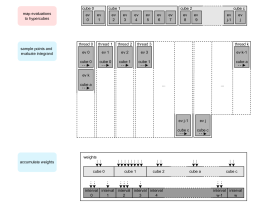
Figure 1: Parallelization diagram of the program in a single GPU setting.

Figure 2: Parallelization diagram of the program in a multi GPU setting.

Although this strategy introduces overhead due to the mapping of evaluations to hypercubes and the accumulation of hypercube weights, it significantly enhances resource utilization. This results in more consistent performance and scalability, particularly for handling highly peaked integrands, which are a focus of the VEGAS+ algorithm.

The process of updating the importance sampling map is inherently sequential and cannot be fully parallelized. Nonetheless, performing this update on the GPU offers a performance advantage over CPU execution. This advantage stems from eliminating the need for memory transfers between the device and the host, thereby enhancing overall efficiency.

3.2 Algorithm Overview and Pseudocode

init( );

  // initialize memory and variables

states $\leftarrow$ setupRNG( );

  // setup RNG states parallel

forall it in iterations do

       foreach w in mapWeights do w $\leftarrow 0$;

        // reset weights parallel foreach w in cubWeights do w $\leftarrow 0$;

        // reset weights parallel evals $\leftarrow$ mapEvalsToCubes(nh);

        // map evaluation to related cube parallelized

       forall state in states do // fill weights parallel

             runs $\leftarrow$ getRuns(evals);

              // get runs for this instance

             mapWeightsTmp, cubWeightsTmp $\leftarrow$ vegasFill(runs, state, map, mapWeights, cubWeights);

              // fill

             mapWeights, cubWeights $\leftarrow$ mapWeights, cubWeights + mapWeightsTmp, cubWeightsTmp;

              // accumulate

            

       end forall

       nh $\leftarrow$ updateEvalsPerCube(cubWeights, beta);

        // compute stratification map parallel

       mapWeights $\leftarrow$ adjustWeights(mapWeights, alpha);

        // smooth map weights parallel

       map $\leftarrow$ updateMap(map, mapWeights);

        // update importance sampling map parallelized

       if it $>$ skip then

             res, sig $\leftarrow$ computeResults(cubWeights);

              // accumulate results from cubes parallel

             results[it], sigmas[it] $\leftarrow$ res, sig;

              // store iteration result

             result, sigma2 = combineIterationsResults(results, sigmas);

              // compute result

            

       end if

      

end forall

clear( );

  // release memory

return result, sigma2;

Algorithm 1 Optimized Algorithm Pseudocode

forall run in runs do

       cub $\leftarrow$ getCube(run);

        // get cube for the run

       x, id $\leftarrow$ getPoint(state, cub);

        // sample point in the cube

       j $\leftarrow$ getJac(id);

        // compute jacobian

       f $\leftarrow$ integrand(x);

        // evaluate integrand

       mapWeights[id] $\leftarrow$ mapWeights[id] + GetMapWeights(j, f);

        // accumulate map weights

       cubWeights[cub] $\leftarrow$ cubWeights[cub] + GetCubWeights(j, f);

        // accumulate cube weights

      

end forall

return mapWeights, cubWeights;

Algorithm 2 VegasFill

The program, outlined in Algorithm 1, starts with the initialization of algorithmic parameters and memory allocation (highlighted in yellow). The random number generators (RNGs) are set up using the cuRAND library XORWOW algorithm. The main loop iterates through the VEGAS algorithm, refining the integral estimation and adapting the grid for enhanced accuracy. The weights of the contribution of each integrand sample, used for updating the map and stratification, are reset (highlighted in green), and every needed integrand function evaluation is mapped to its respective hypercube (highlighted in red), to allow a parallelization with respect to every function evaluation for the successive vegasFill routine (highlighted in blue), outlined in Algorithm 2. For every evaluation in each hypercube, the program generates a random point in the transformed space for which the value of the integrand function is evaluated. Then the Jacobian and weights of that evaluation are computed and accumulated to update the map and stratification parameters.

During the update process (highlighted in green), the accumulated weights are utilized in the updateEvalsPerCube phase to determine the effective number of function evaluations per hypercube. Following this, the map is updated to the new map by computing new parameters. This involves normalization, smoothing and aggregation of the weights with the counts collected in earlier phases.

Simultaneously to the map update, if the iteration index is above a threshold, which is set for the convergence of the map and stratification parameters, the program computes the new estimate of the integral. The results within each hypercube are accumulated in the computeResults routine, to obtain the estimate of the integral for the current iteration, as well as its variance. Subsequently, the results from the previous iterations are combined to obtain a weighted approximation for the integral outcome. After the completion of all iterations, the memory is deallocated (highlighted in orange), and the ultimate integral estimate becomes the program output.

3.3 Implementation details and optimizations

To overcome the parallelization challenges and devise an effective strategy, we must first assess the running time of the various sections of the algorithm and identify areas that require optimization. With this objective in mind, we meticulously examine the implementation details of the algorithm, focusing on techniques to enhance performance and scalability. By understanding the details of the algorithm execution on GPU architectures, we propose optimizations that mitigate bottlenecks and improve overall efficiency.

3.3.1 Program time analysis

Table 1 reports the running time of the different sections of the algorithm. We considered both a computationally “easy” function (Roos&Arnold) and an “intensive” and peaked function (Ridge), defined in Table 3, by examining also the scalability in the number of function evaluations. The majority of the time is spent on the vegasFill routine, where the integrand is evaluated and the results are accumulated. As expected, increasing the number of integrand evaluations translates to a higher total time fraction spent on the filling part, even for computationally “easy” integrands, while it becomes evident for “intensive” integrands. Therefore, it is important to optimize the filling section by allowing a full resource optimization of the integrand evaluations. The other sections benefit also from parallelization but the improvement is minor.

Table 1: Breakdown table of the program running time with multiple number of evaluations of integrand functions of Table 3. The parameters are set to the “def” configuration with reference to Table 2. The color scheme matches the sections of Algorithm 1. The reported time ignores the CUDA context initialization.

integrands	Roos&Arnold				Ridge
integrand evaluations	$10^{7}$	$10^{8}$	$10^{9}$	$10^{10}$	$10^{7}$	$10^{8}$	$10^{9}$	$10^{10}$
init [%]	18.2	10.6	4.4	2.3	4.1	0.9	0.3	0.2
map [%]	10.4	5.2	3.3	3.8	2.2	0.5	0.3	0.3
fill [%]	35.8	70.3	88.0	91.7	89.2	97.7	99.1	99.3
update [%]	33.0	12.0	3.8	2.1	3.9	0.7	0.2	0.1
clear [%]	2.6	1.9	0.5	0.1	0.6	0.2	0.1	0.1
total time [ms]	29.0	91.5	570.8	4697.2	149.4	1123.1	10888.8	108170.2

3.3.2 Optimization of Random Number Generation

The vegasFill procedure, invoked through a kernel launch, is the most computationally demanding part of our algorithm, requiring the highest number of work units. This procedure begins by randomly sampling points in the transformed space, utilizing the cuRAND library XORWOW algorithm for random number generation. Each thread is assigned its own XORWOW state during the setupRNG phase, initialized with a uniform seed but varying sequence numbers.

Given that state initialization is resource-intensive, both in terms of time and memory, it is impractical to allocate a unique state for each evaluation point. To address this, we introduce a batch_size parameter. This parameter specifies the maximum number of threads that the vegasFill kernel can employ, thereby determining the number of XORWOW states that need to be initialized. Consequently, each thread is tasked with generating $\frac{n_{\text{eval}}}{\text{batch\_size}}$ random points.

With each curandState consuming 48 bytes, the upper limit for batch_size is approximately $10^{9}$, subject to the available RAM on the GPU. Additionally, to maximize the utilization of the GPU Streaming Multiprocessors (SMs), the batch_size must be sufficiently large. It is worth noting that the initialization of RNG states is a one-time operation, thereby incurring a fixed computational overhead that is amortized over the entire runtime of the algorithm.

3.3.3 Accumulation and Data Reduction Techniques

The vegasFill procedure leverages AtomicAdd instructions to aggregate weights for both the map and stratification, corresponding to each evaluation specific map interval and hypercube. Reduction operations are also needed for the computation of the integral estimate and variance by accumulating the hypercubes results, and for the map update. These accumulations are further optimized through the use of the CUB software library [36], which offers device-wide specialized functions for array summation, including reduction and prefix-scan operations.

3.3.4 Mitigating Thread Divergence in Hypercube Mapping

Our algorithm parallelization strategy necessitates mapping each integrand function evaluation to its designated hypercube. While GPU-compatible, this operation is prone to thread divergence due to the variable number of evaluations allocated to each hypercube. To counteract this, we implement a conditional approach: the mapping operation is executed on the CPU if the maximum fraction of total evaluations for a single hypercube surpasses a predetermined threshold. Otherwise, it remains on the GPU. For CPU-based mapping, we employ OpenMP parallelization when the evaluation count exceeds a specific value, thereby optimizing multi-threading overhead.

3.3.5 Stream-Based Parallelization for Enhanced Performance

The majority of the computational workload within the main loop is executed on the GPU. To further enhance performance, we employ CUDA streams to parallelize memory operations and computations. Specifically, map updates, which include weight normalization and smoothing, are processed on a high-priority stream. This is separate from the stream responsible for integral estimation, variance calculation, and stratification updates.

3.4 Multi-GPU approach

The implementation enables the execution across multiple GPUs for the vegasFill kernel, responsible for integrand calls and typically consuming the majority of the execution time. Other computations, such as parameter updates and result computation, are handled on a single device. The RNG is initialized by assigning a distinct offset in the random sequence to each GPU device, ensuring an adequate number of random number generations without sequence overlap.

The communication between GPUs is obtained with the cudaDeviceEnablePeerAccess function of the CUDA runtime API, which leverages the NVLink interconnection if possible (available in the SXM design used for testing), to access the peer memory without involving the CPU. Data sharing is achieved through peer-to-peer communication (P2P) for the purpose of merging the fill results. Prior to the kernel call, global memory data structures are replicated to each GPU device, enhancing performance using a tree-like broadcast strategy, which involves $\lceil\log_{2}{n}\rceil$ deviceToDevice data copy steps for $n$ devices. The same strategy is adopted for merging results which requires summing the values into a single array. These data replications and accumulation from multiple GPUs are reported in the parallelization schema in Figure 2.

Utilizing multiple GPUs can be advantageous, particularly with highly computation-intensive integrands, where the data sharing overhead is minimal, and the overall speedup approaches the number of participating devices.

3.5 Performance limitations

The vegasFill kernel accounts for the majority of the program overall execution time. As outlined in the pseudocode 2, it is responsible for the random sampling of the domain points, integrand function evaluation, and weights accumulation with atomic functions. Its computation intensity depends on the integrand device function which is executed in the vegasFill kernel, and typically results in a double-precision floating-point computationally-bound execution. Moreover, the number of required registers, which is also integrand function dependent, limits the occupancy, and small block sizes typically show better overall performance.

Each function evaluation requires the access to the importance sampling map, to locations based on the randomly sampled domain point in each thread. This almost random global memory access introduces latency. A possible approach to mitigate this could be sampling the points beforehand and then order the evaluations to improve coalescing for global memory access to reduce the load on the memory controller.

3.6 Python binding

In order to enhance the program usability and efficiency, we developed a CUDA PyTorch extension using pybind11 [37], a lightweight header-only library that acts as a connection between C++ and Python. This extension enables seamless integration of the existing CUDA C program with the PyTorch framework.

The binding process involves overseeing minimal constant overhead, measurable from 50 to 100 ms, primarily attributed to the just-in-time (JIT) compilation of the integrand function to PTX code, facilitated by the Numba package [38], wherein the integrand is defined as a Numba CUDA device function in Python code. This compilation ensures the integrand function can be linked at runtime to the previously compiled segments of the program. This approach incurs minimal overhead, while enabling a smoother and more straightforward implementation of the algorithm within the Python context.

4 Performance Analysis

In this section, we delve into a comprehensive performance analysis of cuVegas. We benchmark cuVegas against existing implementations, including the original CPU-based Vegas, TorchQuad, and VegasFlow. Our analysis covers multiple dimensions, such as computational speed, memory usage, and the impact of various optimization techniques. The goal is to provide a holistic view of the performance characteristics and advantages of cuVegas.

4.1 Methodology

Table 2: Configuration Parameters

Parameter	Configuration 1 (def)	Configuration 2 (vf)	Configuration 3 (tq)
max_it	20	20	20
skip	0	0	0
max_batch_size	1048576	1048576	1048576
n_intervals	1024	50	computed on n_eval
alpha	0.5	1.5	0.5
beta	0.75	0.75	0.75

Table 3: Test Integrands in This Study

#	Integrand	Dimensions (d)	Function
(1)	Sine Exponential	2D	$f(x)=\sin(x_{1})+\exp(x_{2})$
(2)	Linear	10D	$f(x)=\sum_{i=1}^{d}x_{i}$
(3)	Cosine	10D	$f(x)=\prod_{i=1}^{d}\cos(x_{i})$
(4)	Exponential	10D	$f(x)=\exp(\sum_{i=1}^{d}x_{i}^{2})$
(5)	Roos & Arnold	10D	$f(x)=\prod_{i=1}^{d}\left|4x_{i}-2\right|$
(6)	Morokoff & Caflisch	8D	$f(x)=(1+1/d)^{d}\prod_{i=1}^{d}x_{i}^{1/d}$
(7)	Gaussian	4D	$f(x)=\frac{1}{(2\pi\sigma^{2})^{d/2}}\exp\left(-\frac{\sum_{i=1}^{d}(x_{i}-\mu)^{2}}{2\sigma^{2}}\right);\mu=0.5,\sigma=0.01$
(8)	Ridge	4D	$f(x)=\frac{10000}{\pi^{2}N}\sum_{i=1}^{N}\exp\left(-100{\sum_{j=1}^{d}\left(x_{j}-\frac{i-1}{N-1}\right)^{2}}\right);N=1000$

Table 4: Test implementations

Implementation	#CPUs	#GPUs	Configurations	Details
Vegas (v5.4.2)	2	0	def, vf, tq	official implementation in Cython
Vegas96	96	0	def, vf, tq	Vegas with multiple CPUs
VegasFlow (v1.3.0)	12	1	vf	Tensorflow implementation
TorchQuad (v0.4.0)	12	1	tq	PyTorch implementation
cuVegas	12	1	def, vf, tq	proposed CUDA implementation with Python
cuVegas8	96	8	def, vf, tq	cuVegas with multiple GPUs

Table 5: Test system configuration

System specifications
CPUs	2x AMD EPYC 7643, 96 Threads total, base 2.3 GHz, boost 3.6 GHz
Memory	1 TB DDR4
GPUs	8x Nvidia A100 SXM4, HBM2e 80 GB, 400W
Software	OS Rocky Linux 8.7, CUDA 11.8, TensorFlow 2.13.0, PyTorch 2.0.1

To ensure a fair and comprehensive evaluation, we adopt a multi-faceted methodology. We use three different configurations for our experiments, as detailed in Table 2. These configurations are designed to align with the fixed parameter choices of the baseline implementations, thereby facilitating a more equitable comparison. Particularly TorchQuad and VegasFlow hard-coded configurations have been matched by adjusting the parameters of Vegas and cuVegas. The configurations are “def” (default) that refers to the default parameter choice of both cuVegas and Vegas, “vf” (VegasFlow) that aligns the parameters to those of VegasFlow, and “tq” (TorchQuad) that matches those of TorchQuad. The running time results are computed as the mean over five runs, following a warm-up run.

The implementation versions proposed for testing and the related computational resources are outlined in Table 4, which also shows the parameter configurations tested for each version. We evaluate cuVegas using a diverse set of test integrands and two real-world applications in financial option pricing and quantum physics. The test integrands, listed in Table 3, are chosen to represent a variety of computational complexities and dimensionalities. The system configuration is reported in Table 5.

4.2 VegasFill kernel performance scaling

We analyzed the execution time performance of the vegasFill kernel, when changing the algorithm parameters. For this testing, the parameter configurations reported in Table 6 are used, with the linear integration function (3) over 20 iterations. The default parameters are reported in bold in the table, and represent the fixed configuration when changing a single parameter. The kernel performance is displayed in Figure 3, showing the execution time on the $y$-axis when changing the related parameter on the $x$-axis.

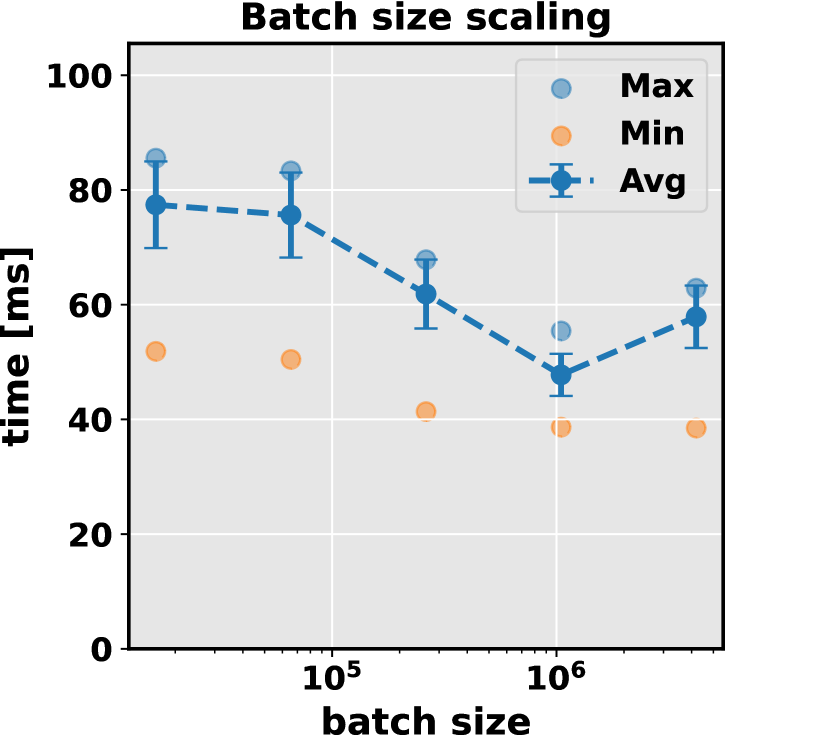
(a)

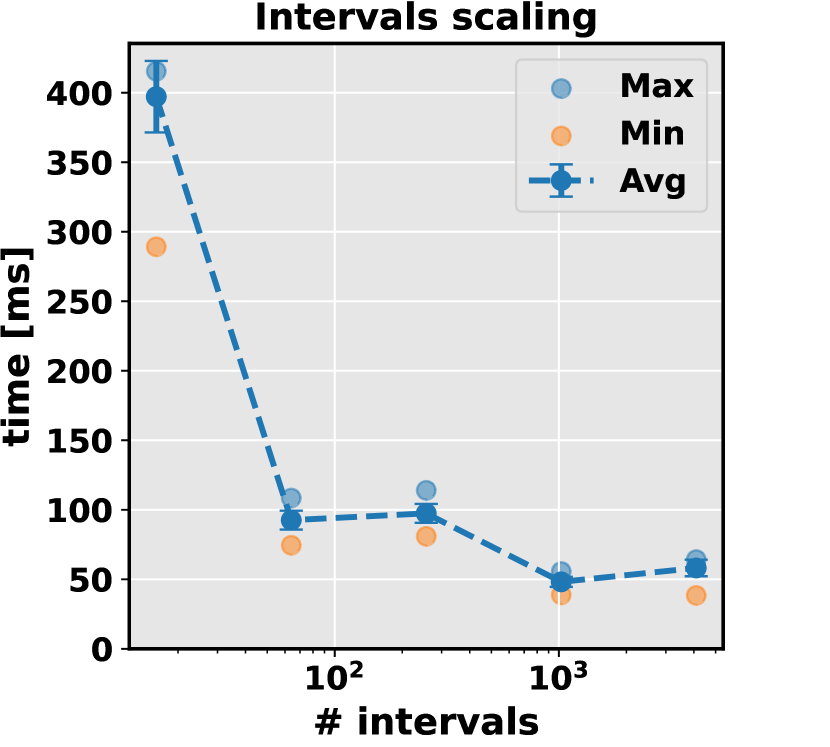
(b)

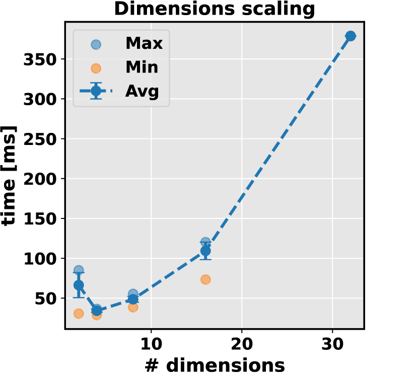
(c)

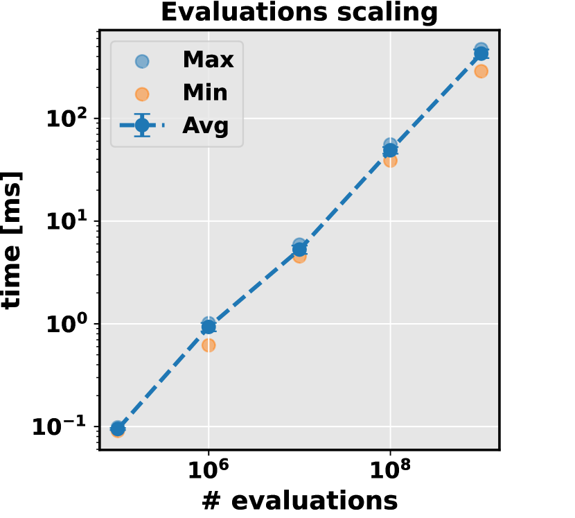
(d)

Figure 3: VegasFill kernel performance scaling, changing algorithm parameters. The testing parameters are reported in Table 6. Blue dots represent mean execution time values of the total kernel calls in the program and bars represent standard error. Orange and light blue dots represent minimum and maximum execution time respectively.

Table 6: Scaling test parameters. The fixed parameters are in reported in bold.

# evaluations	# dimensions	# intervals	batch_size
$2e6$	2	16	16384
$2e7$	4	64	65536
$2e8$	8	256	262144
$2e9$	16	1024	1048576
2e10	32	4096	4194304

The batch_size parameter determines the number of function evaluations conducted by a single thread and subsequently influences the grid size, matching the total number of integrand calls. As shown in the plot in Figure 3(a), a lower value has a detrimental impact on performance, affecting the number of eligible warps and consequently reducing active warps per scheduler. On the other hand, higher values involve a tradeoff within a warp, balancing global memory access randomness and thread serialization for atomic addition. The value 1,048,576 provides good performance and has been used as default for all testing scenarios.

The number of intervals in the VEGAS importance sampling map significantly influences the kernel performance. As illustrated in the plot in Figure 3(b), very low values result in a substantial increase in execution time because all threads atomically sum to the same intervals, causing thread serialization in the map accumulation. Conversely, a very high number of intervals decreases the likelihood of multiple threads writing to the same memory location, yet it leads to increased global memory reads and diminishes the cache hit ratio due to the random nature of intervals. The value 1024 has been chosen as the default, providing a balance between good performance and compatibility with the algorithm itself, resembling the original author’s choice of 1000 as reported in the VEGAS+ paper [8] and in the Cython implementation [28].

As expected, the kernel execution time increases more than linearly with the number of dimensions in the integrand function, as shown in Figure 3(c), due to the additional memory transactions to global memory. Additionally, Figure 3(d) shows that increasing the number of integrand function evaluations leads to an almost linear growth in execution time, as it primarily involves a linear increase in the number of runs for each thread.

4.3 Test integrands benchmark performance

In order to assess the performance of cuVegas in comparison to TorchQuad and VegasFlow, performance evaluations were conducted using seven synthetic benchmarks functions mentioned in Table 3. Specifically integrands 1-7 are considered, excluding Ridge due to its off-scale computational intensity compared to the other functions.

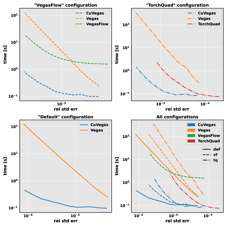
Figure 4: Performance comparison of cuVegas, Vegas, TorchQuad and VegasFlow across seven test functions. On the $y$-axis the average wall-clock time is plotted against the average relative standard error on the $x$-axis. Axes are in log-scale. Lines represent the geometric mean over the seven integrands.

Figure 4 depicts the geometric mean of performance across the seven test integrands. Each data point corresponds to the mean performance of a given implementation with a consistent number of function evaluations across all integrands. We show the performance of the different implementations and configurations reported in Table 4, by showing the results separately for each of the three different configurations, and then the same results combined in a single plot for comparison. The geometric mean of the relative standard error on the $x$-axis is reported against the execution time on the $y$-axis. It is evident that cuVegas exhibits a promising trend. Notably, cuVegas consistently demonstrates lower execution times across a range of relative standard errors, underlining its optimization for rapid computations. Speedups in Table 7 have been computed with respect to the longest run of each version and configuration combination, which result in almost matching error values.

Table 7: Speedup table presenting the relative performance improvements of cuVegas compared to Vegas, TorchQuad, and VegasFlow on the test integrand experiment.

7 Test integrands	Speedup
Version/Config	def	vf	tq
Vegas	278.4x	157.2x	234.8x
VegasFlow	-	21.6x	-
TorchQuad	-	-	6.3x

However, it is worth mentioning that the TorchQuad result does not match the errors of the other versions with the same launch parameters, due to an internal early stopping criterion that stops the computation with a lower number of function evaluations, and resulting in a higher error compared to the other versions. In this case, the speedup is computed comparing the running time of the point with lowest average error achieved by TorchQuad with the time of the next point of cuVegas with a lower error. Considering subsequent points being computed by doubling the number of n_evals and assuming a linearly increasing time, the worst-case penalty is 2x. This puts cuVegas in an unfavorable scenario, but it returns a lower error while still being faster. In addition, it is interesting to observe how the “default” (“def”) parameter configuration of Vegas and cuVegas gives better average performance compared to the “VegasFlow” (“vf”) and “TorchQuad” (“tq”) settings across the benchmark functions. This suggests that the default configuration might be a more sensible parameter choice on average.

4.4 Multi-GPU performance scaling

As described in Section 3.4, our implementation supports multi-GPU execution, with the workload distribution among GPUs centered around the vegasFill part. Therefore, leveraging multiple GPUs can be advantageous particularly when the majority of the program execution time is spent on the filling computation, and the associated data distribution overhead among the GPUs remains insignificant, in line with the principles of Amdahl’s Law. This advantage becomes notable when dealing with computationally intensive integrand functions and a substantial number of function evaluations.

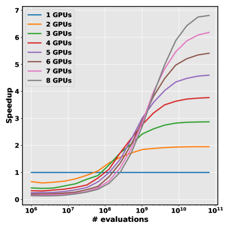
Figure 5: Speedup of multiple GPUs with respect to the single GPU version for the Ridge integrand, varying the number of function evaluations.

Table 8: Speedup and efficiency table presenting the relative performance improvements of multi-GPU runs compared to a single GPU.

# GPUs	Speedup	Efficiency
1	1.00x	1.00
2	1.95x	0.98
3	2.87x	0.96
4	3.77x	0.94
5	4.60x	0.92
6	5.41x	0.90
7	6.18x	0.88
8	6.81x	0.85

As shown by the plot in Figure 5, when considering a sufficiently computationally intensive integrand, such as the Ridge function (defined in Table 3), using multiple GPUs effectively reduces computation time, with enough function evaluations. In Table 8, we report the speedups computed with the highest number of integrand evaluations considered. The table also shows the efficiency computed as $speedup/n_{gpus}$, the average performance of each GPU with repect to the single one. The test has been conducted with the CUDA C implementation of the program. The timing takes into consideration also the CUDA context initialization, which has been measured around 350 ms for each GPU. Therefore it is beneficial to enable the multi-GPU execution of the program when the algorithm running time is considerably larger than the context initialization, to take advantage of the improved performance in the filling part when the overhead is less significant.

4.5 Practical Application Scenarios

We further extend our experiments to two practical applications scenarios, the pricing of Asian Options in Finance and the Path Integrals in Quantum Mechanics.

4.5.1 Pricing of Asian Options

Option pricing is a crucial element in financial markets and involves determining the value of financial derivatives. The Black-Scholes model, commonly used for European options, can be computationally demanding when applied to Asian options, largely due to the high dimensionality involved. Asian options are a type of path-dependent option where Monte Carlo methods are an effective computational tool [3].

We consider the following integrand, which corresponds to the computational representation of an Asian call option:

$$\int e^{-rT}\max(S_{\text{avg}}-K,0)\,\text{d}x$$ (10)

where $e^{-rT}$ is the discount factor, $S_{\text{avg}}$ is the average asset price over the life of the option, $K$ is the strike price, $r$ is the risk-free rate, $T$ is the time to maturity, and $\max(S_{\text{avg}}-K,0)$ represents the payoff of the option. The $S_{\text{avg}}$ is defined as follows:

$$S_{\text{avg}}=S_{0}\exp\left((r-\frac{\sigma^{2}}{2})T+\sigma\sqrt{T}\sum_{i=1}^{n}\text{erf}^{-1}(2x_{i}-1)\sqrt{2}\right)$$ (11)

For further details and derivation, we refer to [3].

Figure 6 showcases the comparative performance of different integration methods for Asian option pricing.

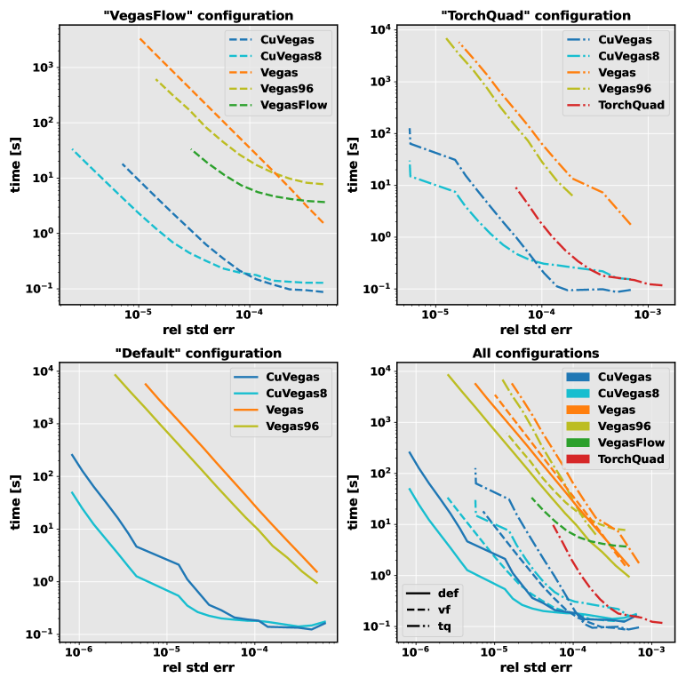
Figure 6: Performance comparison of cuVegas, Vegas, TorchQuad, and VegasFlow on the Asian Option Pricing example integrand. The y-axis plots the average wall-clock time against the average relative standard error on the x-axis, both on log-scale.

Speedups in Table 9 are computed in a “worst case” manner with respect to cuVegas, considering the lowest error point achieved by each configuration and comparing it to the next computed point of cuVegas with a lower error.

Table 9: Speedup table showing the relative performance improvement of cuVegas compared to Vegas, TorchQuad, and VegasFlow in the Asian Option Pricing integrand experiment.

Asian option	Speedup
Config	def		vf		tq
Version	cuVegas	cuVegas8	cuVegas	cuVegas8	cuVegas	cuVegas8
Vegas	1210.2x	4426.9x	382.0x	783.7x	186.6x	772.3x
Vegas96	261.8x	1309.3x	134.1x	497.6x	111.6x	474.5x
VegasFlow	-	-	27.4x	74.6x	-	-
TorchQuad	-	-	-	-	5.0x	13.8x

Our method demonstrates superior efficiency across different configurations, with the “default” (“def”) parameter parameter setup consistently delivering the best performance. This integrand is a computationally intensive function, that effectively harnesses the power of an 8-GPU execution, resulting in noticeable performance gains. It’s important to note that both VegasFlow and TorchQuad experience early termination due to memory saturation.

4.6 Path Integrals in Quantum Mechanics

In quantum mechanics, the path integral formulation extends the concept of the stationary action principle from classical mechanics. In principle, the quantum mechanics of any system (with a classical limit) can be reduced to a problem in multidimensional integration. In one-dimensional quantum mechanics, the evolution of a position eigenstate $|x_{i}\rangle$ from time $t_{i}$ to time $t_{f}$ can be computed using a path integral, We follow the discretization of the path integral procedure described by Lepage [39] as:

$$\langle x|e^{-\tilde{H}T}|x\rangle\approx A\int_{-\infty}^{\infty}dx_{1}\ldots dx_{N-1}e^{-S_{\text{lat}}[x]}$$ (12)

where the lattice action $S_{\text{lat}}[x]$ is given by:

$$S_{\text{lat}}[x]\equiv\sum_{j=0}^{N-1}\left(\frac{m}{2a}(x_{j+1}-x_{j})^{2}+aV(x_{j})\right),$$ (13)

with $x_{0}=x_{N}=x$ the fixed endpoints and $a=T/N$ the grid spacing. We consider a one-dimensional harmonic oscillator, with a potential $V(x)=\frac{x^{2}}{2}$. The integrand high dimensionality and the presence of peaky features make it a suitable candidate to test the performance of our implementation.

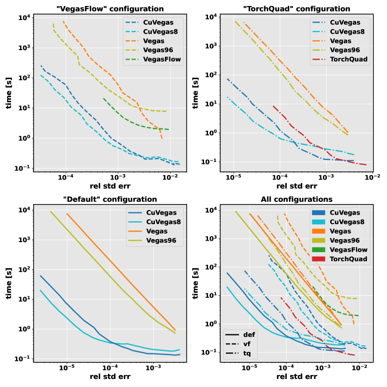
Figure 7: Performance comparison of cuVegas, Vegas, TorchQuad, and VegasFlow on the Feynman Path example integrand. The y-axis shows the average wall-clock time versus the average relative standard error on the x-axis, both in log-scale.

Figure 7 displays a comparative performance analysis of various integration methods applied to the Path integral. The speedups, as detailed in Table 10, are calculated similarly to the previous section, with a focus on cuVegas relative performance.

Table 10: Speedup table showing the performance enhancements of cuVegas compared to Vegas, TorchQuad, and VegasFlow on the Feynman Path integrand experiment.

Feynman path	Speedup
Config	def		vf		tq
Version	cuVegas	cuVegas8	cuVegas	cuVegas8	cuVegas	cuVegas8
Vegas	939.9x	2848.1x	71.1x	182.8x	178.0x	746.5x
Vegas96	145.0x	452.4x	41.3x	93.5x	96.1x	413.4x
VegasFlow	-	-	5.9x	14.3x	-	-
TorchQuad	-	-	-	-	1.8x	5.8x

Our method, cuVegas, demonstrates improved efficiency in different configurations compared to the other methods. This experiment underscores the efficiency of our implementation in handling integrands with complex features. It also raises questions about the potential comparative performance of our method against optimized VEGAS+ implementations for integrals with multiple peaks or other complex structures.

4.7 Impact of Adaptive Stratified Sampling

To assess the specific advantage conferred by adaptive stratified sampling within the VEGAS algorithm framework, we compare the performance of cuVegas with the well-optimized m-CUBES VEGAS implementation [27] that we identified as the best performing implementation of the classical VEGAS algorithm. This comparison particularly aims to elucidate the efficiency gains achievable with adaptive stratification, especially for integrands with highly peaked structures. For testing, we utilize the m-CUBES implementation from Paterno [33], compared to the CUDA C implementation of cuVegas.

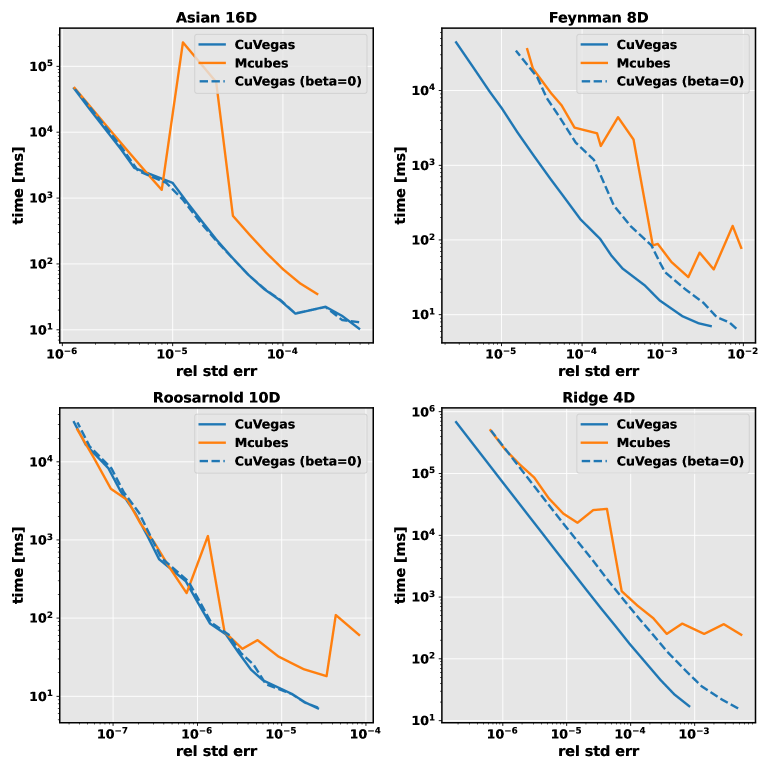
Figure 8: Comparative performance analysis between cuVegas and m-CUBES. On the y-axis the average wall-clock time is plotted against the average relative standard error on the x-axis. Axes are in log-scale.

Figure 8 illustrates the results of this head-to-head assessment. Here, we configured both cuVegas and m-CUBES with consistent parameters ($\alpha=1.5,n_{\text{intervals}}=500$), corresponding to m-CUBES default, and we also matched the $n_{\text{strat}}$ parameter computation to that of m-CUBES, to ensure an equitable comparison. cuVegas was tested under two distinct settings to highlight the impact of adaptive stratification. In detail we enabled adaptive stratification with $\beta=0.25$ (solid line), and disabled it with $\beta=0$ (dashed line).

The test protocol involves running each algorithm for 20 iterations, discounting the first 5 iterations to negate initial stabilization discrepancies in performance recording. We selected a suite of integrands for evaluation, including those with pronounced peaks, such as the Ridge and Feynman integrands.

The findings are clear: the performance of cuVegas, when leveraging adaptive stratification ($\beta=0.25$), improves markedly for integrands with significant peak characteristics, confirming the feature value in these challenging scenarios. For more uniformly behaving integrands, the performance distinction between stratification-enabled and -disabled is minimal, with m-CUBES maintaining a performance parity with cuVegas across a higher number of function evaluations.

4.8 Discussion

Our testing involved a comprehensive set of synthetic benchmark functions and real-world applications, including Asian option pricing in finance and Feynman path integrals in quantum physics. Using equivalent parameter configurations across implementations ensured fair and consistent comparisons. The results showed that cuVegas is consistently faster than both CPU-based and other GPU-based alternatives across a variety of computational complexities and dimensionalities.

In real-world scenarios like Feynman path integrals and Asian options, cuVegas demonstrated a clear advantage. In the context of Asian option pricing, our implementation achieved faster computation times and reduced error margins, proving its efficacy in financial computations where rapid calculations are necessary for real-time trading and risk management. Similarly, Feynman path integrals in quantum physics showed cuVegas’s ability to handle complex integrands and provide precise calculations, which are crucial for advancements in science and industry.

The default configuration consistently outperformed the VegasFlow and TorchQuad fixed settings, indicating that our default parameter setup is generally more effective across different scenarios. Nevertheless, cuVegas allows users to configure and adapt its parameters, offering flexibility beyond fixed configurations. Additionally, cuVegas excels at managing complex integrands, especially those with multiple peaks or irregular structures, thanks to the adaptive stratified sampling approach of VEGAS+. In these situations, the program demonstrated its stability and efficiency in balancing workload across threads for various integrand scenarios.

The multi-GPU performance scaling experiments further highlight cuVegas’s scalability. Our implementation shows substantial performance gains when leveraging multiple GPUs, especially for computationally intensive tasks. This capability is crucial for applications requiring large-scale simulations and high computational throughput.

Despite these significant improvements, cuVegas has some limitations. The memory requirements for large-scale integrands can be substantial, particularly when scaling across multiple GPUs. Additionally, performance gains are primarily observed with complex integrands, while simpler scenarios might benefit from further optimization, as the overhead of advanced sampling techniques may not justify the performance gains.

Future work could explore reducing computational costs for simpler integrands and expanding support for more diverse hardware configurations, including mixed-precision calculations and distributed computing frameworks, to extend cuVegas’s applicability even further [40].

5 Conclusions

In this work, we introduced cuVegas, a CUDA-based implementation of the Vegas Enhanced algorithm, and provided a comprehensive performance analysis against existing CPU-based and GPU-based implementations. Our findings clearly demonstrate the significant advantages of leveraging GPU computing for Monte Carlo integration tasks, with cuVegas achieving speedups of one to three orders of magnitude over traditional CPU implementations. Moreover, when compared to existing Python GPU frameworks [32, 29], cuVegas exhibits a speedup of 2x to 20x, underscoring its superior efficiency, outperforming the other implementations across a variety of integrands and dimensionalities.

Against native CUDA C implementations [33], cuVegas matches performance for standard integrands and exhibits a factor of five speedup for integrands benefiting from adaptive stratified sampling. This highlights the algorithm’s effectiveness in handling complex integration tasks, further reinforcing its utility across various applications.

Notably, cuVegas supports multi-GPU setups, enhancing its capability to process complex integrals. The inclusion of Python bindings also simplifies the usage of the method, making it accessible to a broader audience and facilitating integration with existing scientific workflows.

Extensive evaluation on benchmark functions and real-world scenarios like Feynman path integrals in quantum physics and Asian option pricing in financial mathematics, indicates that our method’s strengths are consistent across various domains. This consistency provides confidence in cuVegas’s applicability to a wide range of complex integration tasks, from financial modeling to quantum physics simulations.

In conclusion, the implementation of the Vegas Enhanced algorithm on GPUs is a promising advancement that enhances computational power and applicability across numerous fields. By leveraging GPU parallelism, our approach provides a scalable and efficient solution for high-dimensional numerical integration challenges. This capability opens the door to more advanced analyses and practical applications across different fields and it lays the groundwork for further exploration and development.

References

- [1] Philip J Davis and Philip Rabinowitz “Methods of numerical integration” Courier Corporation, 2007
- [2] M.H. Kalos and P.A. Whitlock “Monte Carlo Methods”, Monte Carlo Methods Wiley, 2008 URL: https://books.google.it/books?id=IEBjLmmbzDMC
- [3] Paul Glasserman “Monte Carlo Methods in financial engineering” Springer, 2010
- [4] A. Gelman et al. “Bayesian Data Analysis, Third Edition”, Chapman & Hall/CRC Texts in Statistical Science Taylor & Francis, 2013 URL: https://books.google.it/books?id=ZXL6AQAAQBAJ
- [5] R.L. Burden, J.D. Faires and A.M. Burden “Numerical Analysis” Cengage Learning, 2015 URL: https://books.google.it/books?id=9DV-BAAAQBAJ
- [6] Paola Favati, Grazia Lotti and Francesco Romani “Algorithm 691: Improving QUADPACK automatic integration routines” In ACM Trans. Math. Softw. 17.2 New York, NY, USA: Association for Computing Machinery, 1991, pp. 218–232 DOI: 10.1145/108556.108580
- [7] Reuven Y Rubinstein and Dirk P Kroese “Simulation and the Monte Carlo method” John Wiley & Sons, 2016
- [8] G. Lepage “Adaptive multidimensional integration: vegas enhanced” In Journal of Computational Physics 439 Elsevier BV, 2021, pp. 110386 DOI: 10.1016/j.jcp.2021.110386
- [9] J. Liu “Monte Carlo Strategies in Scientific Computing” In Springer Series in Statistics, 2001
- [10] G Peter Lepage “A new algorithm for adaptive multidimensional integration” In Journal of Computational Physics 27.2, 1978, pp. 192–203 DOI: https://doi.org/10.1016/0021-9991(78)90004-9
- [11] B.. Kersevan and E. Richter-Was “The Monte Carlo event generator AcerMC versions 2.0 to 3.8 with interfaces to PYTHIA 6.4, HERWIG 6.5 and ARIADNE 4.1” In Comp. Phys. Comm. 184, 2013, pp. 919–985
- [12] J. Alwall “The automated computation of tree-level and next-to-leading order differential cross sections, and their matching to parton shower simulations” In JHEP 07, 2014, pp. 079
- [13] T. Aoyama, M. Hayakawa, T. Kinoshita and M. Nio “Complete Tenth-Order QED Contribution to the Muon g – 2” In Phys. Rev. Lett. 109, 2012, pp. 111808
- [14] G. Garberoglio and A.. Harvey “Path-Integral calculation of the third virial coefficient of quantum gases at low temperatures” In J. Chem. Phys. 134, 2011, pp. 134106
- [15] G. Campolieti and R. Makarov “Pricing Path-Dependent Options on State Dependent Volatility Models with a Bessel Bridge” In Int. J. Theor. Appl. Finance 10, 2007, pp. 51–88
- [16] P. Serra, A. Heavens and A. Melchiorri “Bayesian Evidence for a cosmological constant using new high-redshift supernova data” In Mon. Not. R. Astron. Soc. 379, 2007, pp. 169–175
- [17] J.. Sanders “Probabilistic model for constraining the Galactic potential using tidal streams” In Mon. Not. R. Astron. Soc. 443, 2014, pp. 423–431
- [18] K. Gultekin “The M- and M-L Relations In Galactic Bulges, and Determinations of their Intrinsic Scatter” In Astrophys. J. 698, 2009, pp. 198–221
- [19] F.. Atay and A. Hutt “Neural Fields with Distributed Transmission Speeds and Long-Range Feedback Delays” In SIAM J. Appl. Dyn. Sys. 5, 2006, pp. 670–698
- [20] J.. Dehesa et al. “Quantum entanglement in helium” In J. Phys. B: At. Mol. Opt. Phys. 45, 2012, pp. 015504
- [21] Wen-mei W. Hwu “GPU Computing Gems Emerald Edition” San Francisco, CA, USA: Morgan Kaufmann Publishers Inc., 2011
- [22] John Owens et al. “GPU computing” In Proceedings of the IEEE 96, 2008, pp. 879–899 DOI: 10.1109/JPROC.2008.917757
- [23] J. Kanzaki “Monte Carlo integration on GPU” In The European Physical Journal C 71.2 Springer ScienceBusiness Media LLC, 2011 DOI: 10.1140/epjc/s10052-011-1559-8
- [24] T. Hahn “Cuba—a library for multidimensional numerical integration” In Computer Physics Communications 168.2, 2005, pp. 78–95 DOI: https://doi.org/10.1016/j.cpc.2005.01.010
- [25] Brian Gough “GNU Scientific Library Reference Manual - Third Edition” Network Theory Ltd., 2009
- [26] Balasubramanian Narasimhan et al. “cubature: Adaptive Multivariate Integration over Hypercubes” R package version 2.1.0, 2023 URL: https://bnaras.github.io/cubature/
- [27] Ioannis Sakiotis et al. “m-CUBES An efficient and portable implementation of multi-dimensional integration for gpus” In CoRR abs/2202.01753, 2022 arXiv: https://arxiv.org/abs/2202.01753
- [28] Peter Lepage “gplepage/vegas: vegas version 5.4.2” Zenodo, 2023 DOI: 10.5281/zenodo.8175999
- [29] Stefano Carrazza and Juan M. Cruz-Martinez “VegasFlow: accelerating Monte Carlo simulation across multiple hardware platforms” In Comput. Phys. Commun. 254, 2020, pp. 107376 DOI: 10.1016/j.cpc.2020.107376
- [30] Juan Cruz-Martinez and Stefano Carrazza “N3PDF/vegasflow: vegasflow v1.0” Zenodo, 2020 DOI: 10.5281/zenodo.3691926
- [31] Pablo Gómez, Håvard Hem Toftevaag and Gabriele Meoni “torchquad: Numerical Integration in Arbitrary Dimensions with PyTorch” In Journal of Open Source Software 6.64 The Open Journal, 2021, pp. 3439 DOI: 10.21105/joss.03439
- [32] P. Gómez, H. Hem Toftevaag and G. Meoni “torchquad: Numerical Integration in Arbitrary Dimensions with PyTorch, TensorFlow & JAX (v0.4.0)” Zenodo, 2023 DOI: 10.5281/zenodo.8041976
- [33] Marc Paterno “Numerical Integration on GPUs”, 2023 URL: https://github.com/marcpaterno/gpuintegration
- [34] Yongcheng Wu “CIGAR” In GitHub repository GitHub, https://github.com/ycwu1030/CIGAR, 2020
- [35] Emiliano Tolotti “cuVegas” In GitHub repository GitHub, https://github.com/emiliantolo/cuvegas, 2024
- [36] Nvidia “CUB” Nvidia, 2023 URL: https://nvlabs.github.io/cub/
- [37] Wenzel Jakob, Jason Rhinelander and Dean Moldovan “pybind11 — Seamless operability between C++11 and Python”, 2023 URL: https://github.com/pybind/pybind11
- [38] Siu Kwan Lam, Antoine Pitrou and Stanley Seibert “Numba: A LLVM-Based Python JIT Compiler” In Proceedings of the Second Workshop on the LLVM Compiler Infrastructure in HPC, LLVM ’15 Austin, Texas: Association for Computing Machinery, 2015 DOI: 10.1145/2833157.2833162
- [39] G. Lepage “Lattice QCD for Novices” In arXiv preprint hep-lat/0506036, 2005 URL: http://arxiv.org/abs/hep-lat/0506036
- [40] Marc Baboulin et al. “Accelerating scientific computations with mixed precision algorithms” 40 YEARS OF CPC: A celebratory issue focused on quality software for high performance, grid and novel computing architectures In Computer Physics Communications 180.12, 2009, pp. 2526–2533 DOI: https://doi.org/10.1016/j.cpc.2008.11.005