Parametric Sensitivity Analysis for Models of Reaction Networks within Interacting Compartments
Abstract
Models of reaction networks within interacting compartments (RNIC) are a generalization of stochastic reaction networks. It is most natural to think of the interacting compartments as “cells” that can appear, degrade, split, and even merge, with each cell containing an evolving copy of the underlying stochastic reaction network. Such models have a number of parameters, including those associated with the internal chemical model and those associated with the compartment interactions, and it is natural to want efficient computational methods for the numerical estimation of sensitivities of model statistics with respect to these parameters. Motivated by the extensive work on computational methods for parametric sensitivity analysis in the context of stochastic reaction networks over the past few decades, we provide a number of methods in the RNIC setting. Provided methods include the (unbiased) Girsanov transformation method (also called the Likelihood Ratio method) and a number of coupling methods for the implementation of finite differences. We provide several numerical examples and conclude that the method associated with the “Split Coupling” provides the most efficient algorithm. This finding is in line with the conclusions from the work related to sensitivity analysis of standard stochastic reaction networks. We have made all of the Matlab code used to implement the various methods freely available for download.
Keywords: coupling methods, stochastic reaction networks, RNIC models.
AMS subject classifications: 60J27, 60J28, 60H35, 65C05
1 Introduction
The last few decades have seen a large amount of research focused on utilizing stochastic reaction networks to understand myriad processes, including gene regulatory networks, viral and bacterial infections, and more [33, 11, 13, 16, 22, 26, 27, 29, 34]. The standard mathematical model for a stochastic reaction network treats the system as a continuous-time Markov chain on , where is the number of species of the system, with reactions determining the state transitions of the model. Such mathematical models are typically used under the assumption that the real-world system being studied resides within a “well-stirred” environment. See [9, 10] for a general (mathematical) introduction to such models. These models are often termed “Gillespie” models in various subfields of the biosciences due to the work by Dan Gillespie in the mid-1970s [19, 20].
The assumption that the system of interest resides within a well-stirred environment can be generalized in numerous ways, depending on the problem being studied. For example, in some situations it may be natural to track the position of individual molecules, either in a discretized space or a continuous space setting [14, 1, 23, 17]. Another approach, and the one we take here, is to assume the existence of multiple interacting “compartments” (or cells) each of which contains an evolving copy of a given stochastic reaction network. This approach is useful in numerous modeling scenarios including the dynamics of membrane-bound organelles [35], the study of clustering proteins [32], and the dynamics of clonal cells during their development [31]. In [15], a modeling framework was formalized for this type of system which can be briefly summarized in the fallowing manner.
-
•
There are a number of “compartments” (one can think of them as cells) that are interacting dynamically. Following the language of [15], the four types of interactions for the compartments are: (i) inflows (compartments spontaneously appear at some rate), (ii) outflows (compartments spontaneously disappear, or die), (iii) coagulation or the merger of two compartments, and (iv) fragmentation (a compartment divides into two compartments).
-
•
Each compartment contains an evolving copy of a given stochastic reaction network. The stochastic reaction networks evolve independently between compartment events/interactions.
-
•
When a compartment appears, the initial state of its contents is chosen from a given distribution on . We will later denote this distribution by .
-
•
When a compartment disappears, its contents disappear as well.
-
•
When compartments merge, their contents combine.
-
•
When a compartment fragments, the contents are randomly split between the two compartments.
A first comprehensive mathematical analysis of these models (with results related to such basic questions as transience, recurrence, explosiveness, stationary behavior, etc.) can be found in [6].
Before continuing, we answer a potential question. Thinking of the compartments as cells, the transitions for arrivals, departures/deaths, and fragmentation all make biological sense. However, coagulation feels different. Therefore, it is reasonable to ask: in what circumstances is it reasonable to include coagulation in the model? In [15], Duso and Zechner, who are much closer to the biology than us, say the following: “Coagulation–fragmentation processes form an important class of models to describe populations of interacting components (15), which have been used to study biological phenomena at different scales, including protein clustering (29), vesicle trafficking (30–32), or clone-size dynamics during development (33)” (Citations from [15]). For example, in [31] (citation 33 in [15]), the authors state “Merger and fragmentation of labelled cell clusters occur naturally because of large-scale tissue rearrangements during the growth and development of tissues.” Of course, if cell coagulation is not relevant to a particular model, then the rate of that transition type should be set to zero.
These RNIC models have many parameters: those associated with the reaction network (evolving within each compartment), the parameters associated with the evolving compartment model, the parameters of the initial distribution for when compartments appear, etc. When working with any mathematical model a critical question is: how sensitive is the model to perturbations in its parameters? As we are dealing with a stochastic process, the most natural way to pose this question is as follows: what are the derivatives of the relevant expectations of the model? Here the “relevant expectations” will depend upon the model being studied and the questions being posed, but could include expected numbers of certain species (summed over all the compartments, perhaps) at a given time, the probability of the model being in a certain region of state space at a given time, etc. The study of such derivatives is typically called parametric sensitivity analysis and plays a critical role in the computational study of stochastic models in all fields that utilize them [12, 24, 28, 3].
In this paper, we provide a number of computational methods that estimate derivatives of expectations of RNIC models. In particular, we provide a Girsanov transformation method (also termed a likelihood transformation method), which is unbiased, and a number of finite difference methods, which typically have very small biases. We do not provide any pathwise differentiation methods (also termed Infinitesimal Perturbation Analysis) as stochastic reaction networks (and, hence, RNIC models) nearly always have “interruptions,” ensuring these methods are not valid in this context [21, 36]. The finite difference methods provided here are each based off a different coupling strategy taken from the computational stochastic reaction network literature. These couplings are: Common Random Variables (CRV) (i.e., using the same seeds for the random number generator), the Common Reaction Path (CRP) method [30], and the Split Coupling method [3, 5]. We provide a number of numerical examples, with perturbations in both the chemical and compartment parameters, and conclude that the Split Coupling should be the method of choice in nearly all scenarios. We explicitly point out here that decades of thought and effort has gone into developing these various methods for the “standard” stochastic reaction networks and a key contribution of the current work is to determine how to modify these to the RNIC framework, and to do so in a single work so that fair comparisons are possible.
The remainder of the paper is arranged as follows. In Section 2, we formally introduce the relevant mathematical models, including both the standard model of stochastic reaction networks and the RNIC model. In Section 3, we provide various computational methods for the estimation of parametric sensitivities. In particular, we demonstrate how to implement the Girsanov transformation method and the Split Coupling in the RNIC context. This is a key contribution of this work. In Section 4, we provide a number of computational examples. Finally, in Section 5, we discuss our findings. In particular, we conclude that the method associated with the Split Coupling of [3, 5] is the most efficient in the RNIC setting and should be used in nearly all circumstances. In the appendix Section A, and for the sake of completeness, we give a very brief introduction to Monte Carlo methods in the context of estimating parametric sensitivities with finite difference methods. In the appendix Section B, we provide a number of algorithms that are utilized for the standard stochastic reaction network models (as introduced in Section 2).
2 Mathematical models
We first introduce the standard model for stochastic reaction networks in Section 2.1. Next, in Section 2.2, we introduce the RNIC model. We also provide in Algorithm 1 a pseudo-algorithm for generating a single trajectory of an RNIC model.
2.1 Stochastic reaction networks
We begin with the definition of a reaction network.
Definition 2.1.
A reaction network is a triple of non-empty, finite sets, usually denoted .
-
1.
Species, : the components whose abundances we wish to model dynamically.
-
2.
Complexes, : non-negative integer linear combinations of the species.
-
3.
Reactions, : a binary relation on the complexes. The relation is often denoted “”.
For with , we call and the source and product complexes of that reaction, respectively. We write for the complex with all zero coefficients.
An example demonstrates the terminology.
Example 2.1.
Consider a standard model of transcription and translation, with protein dimerization (see Example 2.4 in [10]):
| (Transcription) | ||||
| (Translation) | ||||
| (Degradation of mRNA) | ||||
| (Degradation of protein) | ||||
| (Dimerization) | ||||
| (Degradation of dimer) |
where represents mRNA, represents protein, and represents dimer. We are assuming the cell has one gene, and so we suppress that species.
For this model, the species are
the complexes are
and the six reaction types are as above, .
From the reaction graph, a number of dynamical systems can be constructed. These include discrete stochastic models, diffusion models, reaction-diffusion models (which also require a characterization of the space within which the system resides), and ODE models. We introduce the standard discrete-space, continuous-time stochastic model here, and point to [10] for a more thorough introduction.
To fix notation, we assume there are species, which we label as . We will denote the process by , so that gives the state at time . Therefore, is a vector giving the abundance of molecules of each species at the specified time. The state transitions for the model are then determined by the different reactions. For the th reaction, we let and be the vectors whose th component gives the multiplicity of species in the source and product complexes, respectively, and let give the transition intensity, or rate, at which the reaction occurs. (Note that in the biological and chemical literature transition intensities are referred to as propensities [19, 20].) If the th reaction occurs at time , then the old state, , is updated by addition of the reaction vector
| (1) |
and the new state is given as . Here, by we mean the left-sided limit . For example, if a model consists of the three species and if the reaction type takes place, then we would update with
Denoting the number of times the th reaction occurs by time as , simple bookkeeping implies
where the sum is over reactions. Note that each is a counting process (starts at 0 and can only change by increases of size ) with intensity . Letting be independent unit-rate Poisson processes, Kurtz’s representation (which is useful for both analysis and computation) has [25, 10]. Hence, the model satisfies the the following equation, which is often termed the random time change representation of Kurtz:
| (2) |
where the sum is over the reaction types. We will denote a family of such models, parameterized by (which, in the case of stochastic mass-action kinetics—see below—is most likely a rate constant of the system), as
| (3) |
The most common, though certainly not the only, choice of intensity function is that of stochastic mass-action kinetics. The stochastic form of the law of mass-action says that for some constant the rate of the th reaction is
| (4) |
where is the th component of the source complex .111We note that in [6], the intensity functions were defined slightly differently as The rate constants are typically placed next to their reaction arrow in the reaction graph, as in (5) or (9), which are found later in the paper.
2.2 Reaction Network within Interacting Compartments (RNIC)
We have already introduced the basic idea of the RNIC model in the introduction. Here we fill in the necessary technical details. We point the interested reader to [6] for a full mathematical introduction (including myriad theoretical results) for the model. Note that the detailed choices we specify in this section, and especially in the pseudo-code provided at the end, are those that we make in our Matlab code for the simulation of these processes (and which is freely available).
As mentioned in the introduction, the RNIC model consists of interacting compartments, each of which contains an evolving copy of a given reaction network. Therefore, we begin by denoting the reaction network by
When assuming stochastic mass-action kinetics, we will denote the set of rate constants by , and denote
Turning to the compartment model, the number of compartments is modeled as a stochastic reaction network as well. Specifically, by
| (5) |
with stochastic mass-action kinetics and where the rate constants have been placed next to the respective reaction arrows with the rate constant for inflows, for exits, for fragmentations, and for coagulations (following the terminology of [15] and [6]). We will denote by the compartment reaction network (5) (where we have also expanded the set to include the rate constants for both the reaction network and the compartment model).
Denote by the number of compartments at time . Then, following (2), the compartment model satisfies the stochastic equation
where and are independent unit-rate Poisson processes.
Between the transition times of the Markov process each compartment contains an independently evolving copy of the stochastic reaction network . We numerically order the compartments and for we denote the state of the stochastic reaction network evolving in the th compartment by . We now simply need to specify what happens to the model at the transition times of . We do that below. We point out that all choices of random variables below are independent from each other and independent from the Poisson processes , and mentioned above.
We will assume that a transition for takes place at time . Hence, before the transition there are exactly compartments (where, again, denotes a limit in from the left). We now consider each of the four possible transition types for . We note that the names of certain indices below, including IndexDel, IndexFrag, ri1, and ri2, are the names of the indices utilized in the Matlab code we are making available.
-
1.
Case 1: a new compartment arrives at time . In short, in this case we append a new compartment at the end of our list and initialize the stochastic reaction network via a probability distribution we denote by . Specifically, we do the following.
-
(a)
Set .
-
(b)
Set for all (that is, the reaction networks within each of the existing compartments remain the same).
-
(c)
Initialize the stochastic reaction network of the new compartment. The state of the new compartment will be drawn from a fixed probability measure on , where is the number of species in the reaction network model .
-
(a)
-
2.
Case 2: a compartment exits at time . In short, in this case, we delete a compartment at random and shift the indices of the remaining compartments down appropriately. Specifically, we do the following.
-
(a)
Choose from uniformly; with the chosen index called IndexDel.
-
(b)
For , set .
-
(c)
For , set (that is, we shift indices by 1).
-
(d)
Set .
-
(a)
-
3.
Case 3: a compartment fragments into two at time . In short, in this case, one compartment is chosen to divide. Each molecule of each species is chosen to either remain in the old compartment, or be placed into a new compartment numbered as . Specifically, we do the following.
-
(a)
Set .
-
(b)
Choose from uniformly, with the chosen index called IndexFrag.
-
(c)
For each species , we generate a binomial random variable with parameters (abundance of species in compartment IndexFrag) and .
-
(d)
The values given by the binomial random variables determine the state of (i.e., they are the molecules that remain).
-
(e)
The state of is the binomials (i.e., these are the molecules that moved).
-
(a)
-
4.
Case 4: a coagulation (merger). In short, in this case two compartments are chosen to merge. The contents are combined into one of the compartments and the other is deleted. Specifically, we do the following.
-
(a)
Choose two indices, uniformly, with .
-
(b)
Combine the contents into compartment ri1:
-
(c)
Delete the compartment ri2 as detailed in Case 2 above.
-
(d)
Set .
-
(a)
In agreement with the article [6], we will denote the stochastic process associated to the full RNIC model by (where the label “sim” denotes that this representation of the model is natural for simulations). Hence, determines and each of , , for each . The process is a continuous-time Markov chain with discrete state space , the space of finite tuples of [6, Lemma 2.5]. For example, if and a possible realization of is
which would have , and . When we wish to denote a parameterized family, we will once again append our processes with a : , , and .
Having specified the model, we can present a pseudo-code for how to simulate a given RNIC process. In the pseudo-code below, we do not specify the algorithms being used to simulate or the stochastic reaction networks within each compartment, as we leave that up to the implementer. Natural choices are the Gillespie algorithm [19, 20] or the next reaction method [2, 18]. These can both be found in Appendix B. We will denote the initial distribution of by , the initial distribution for the initial compartments by , and the initial distribution for compartments that arrive as . Note that it is possible, though not necessary, that .
Algorithm 1 (Pseudo-code for simulating an RNIC model, ).
Given: a stochastic reaction network , the compartment model (5), the parameters of the model , which consist of the rate constants for , the parameters of the compartment model , and initial distributions , , and .
Repeat steps 4 – 8 until a stopping criteria is reached. All calls to random variables are independent from all others.
-
1.
Determine via .
-
2.
For each determine via .
-
3.
Set .
- 4.
- 5.
-
6.
Determine which type of transition occurs for the compartment model at time .
-
7.
Update the model as detailed in the four cases listed above depending upon which type of transition takes place for the compartment model.
-
8.
Set .
3 Methods for parametric sensitivities
We provide a number of methods for the estimation of parametric sensitivities of RNIC models. In Section 3.1, we provide the (unbiased) Girsanov or Likelihood Ratio method in this setting. In Section 3.2 we provide a number of coupling methods for the implementation of finite differences.
3.1 Likelihood Ratio, or Girsanov, transformation method
We provide the Likelihood Ratio method [12], often called the Girsanov transformation method in the biosciences [28], for the RNIC model when the perturbed parameters are rate constants for either the compartment model, , or the chemical model . There are other possible parameters to consider, such as any parameters associated with the distributions , , or . However, those cases can be handled in a similar, and straightforward, manner.
While we do not provide formal mathematical justification for this method here (see [12]) we do try to provide some intuition by explaining how the method works for the estimation , where is a standard stochastic reaction network and is some terminal time. Extension to the RNIC model is then relatively straightforward.
Consider a reaction network with intensity functions , which are parameterized by , and associated jump directions . Denote . The key point for this method is that it proceeds by finding an appropriate function , often called the “weight function,” so that
One can then estimate the derivative via Monte Carlo with independent samples of .
The function is found by taking the derivative, with respect to the parameter , of the logarithm of the density of the process up to time . For example, suppose that is a particular path of the process (that one may have simulated, for example). Then, for this particular path, let , be the number of reactions that have taken place up to time , be the time of the th transition (for ), be the index of the reaction type that takes place at time , and be the holding time in state . Thinking in terms of the Gillespie algorithm, i.e., which reaction happens next and when that reaction takes place, which are a discrete event and an exponential holding time, respectively, it is then relatively straightforward to see [12, 28] that the density of the process at time is proportional to
Taking logarithms and derivatives is now straightforward, and we have
Note that in the case of stochastic mass-action kinetics with , we have the simple expressions
An implementation of this method is given in Algorithm 6 in Appendix B.
We now turn back to the RNIC model. We will denote our statistic of interest as , where is the state of the RNIC model at time and is a function of interest. We will denote by the generated weight function. Hence, we utilize the algorithms below to estimate by averaging the independent realizations , with enumerating the independent calls to the algorithm.
In fact, the details above pertaining to the Girsanov method for standard stochastic reaction networks allow us to immediately provide the Girsanov transformation method when the perturbed parameter is one of the rate constants associated with the compartment model, . This is because the compartment model can be simulated with no knowledge of the internal reaction networks. Specifically, the following pseudo-algorithm works:
We turn to the case when the parameter of interest is in the reaction network . Because the reaction networks within each compartment evolve independently, we may sum the representative weight functions from the calls to between compartment events. Hence, simulation in this case is also straightforward. However, since this situation is different from what is standard, we provide a pseudo-algorithm.
Algorithm 2 (Girsanov transformation method if the perturbed parameter is from the reaction network model, ).
Given: a stochastic reaction network , the compartment model (5), the parameters of the model , which consist of the rate constants for and the parameters of the compartment model , initial distributions , , and .
All calls to random variables are independent from all others.
-
1.
Determine via .
-
2.
For each determine via .
-
3.
Set and set .
-
4.
Using Gillespie’s Algorithm 4, determine the time until the next transition of the compartment model, .
-
5.
If , set and break after step 6.
-
6.
Using the reaction network Girsanov transformation Algorithm 6, for all simulate from time to time and let denote the output weight function.
Set .
-
7.
Determine which type of transition occurs for the compartment model at time .
-
8.
Update the RNIC model as detailed in the four cases listed in Section 2.2 depending upon which type of transition takes place for the compartment model.
-
9.
Set .
Output and .
3.2 Finite difference methods
As detailed in Appendix A, the basic idea of finite difference methods is to use the following straightforward approximation,
| (6) | ||||
where the key fact is that and are generated on the same probability space. That is, and are coupled so that is reduced.222In the appendix we introduced the centered finite difference, whereas here we are using the forward difference. The variance is not affected by this choice and so we utilize the less notationally cumbersome choice here.
We will use four basic coupling methods, each with different “flavors” depending on what type of parameter is being perturbed. We begin with a simple introduction to each.
Method 1: Independent Samples. This is straightforward. You simply generate the processes independently. This should be viewed as the base case.
Method 2: Common Random Variables (CRV). This is nearly as simply as generating the processes independently and consists of simply reusing the seed of your random number generator for the calls to the different processes. Alternatively, and equivalently, you can pre-generate vectors of uniform[0,1]—or other—random variables that can be used to simulate the process.
Method 3: Common Reaction Path method (CRP). This method was developed for standard stochastic reaction networks, so we first explain it in that language. Hence, consider a stochastic reaction network with jump directions and intensity functions , which are parameterized by . The Common Reaction Path method for such a process couples and by reusing the unit-rate Poisson processes in (3) [30]. That is, and are coupled in the following manner,
where the key point is that the same unit-rate Poisson processes, , are utilized for both and .
Method 4: Split Coupling (SC). As with the method above, this method was developed for standard stochastic reaction networks, so we first explain it in that context. Thus, consider a stochastic reaction network with jump directions and intensity functions , which are parameterized by . The Split Coupling method for such a process couples and by constructing them in the following manner [3, 5],
| (7) | ||||
where are all independent unit-rate Poisson processes. Note that both processes reuse the jump processes associated with the Poisson processes . For the purposes of this paper, we will simply note that the Split Coupling works (in that and have the correct distributions) because of the fact that Poisson processes are additive in that if and are unit-rate Poisson processes, and if are integrable functions, then is equal in distribution to .
The question now is how we implement these basic methods in the RNIC setting. There are two distinct cases to consider: whether the parameter being perturbed is a compartment parameter (, or ) or is a parameter from the reaction network (e.g., a rate constant for stochastic mass-action kinetics). One case is demonstrably more straightforward, and so we start with that.
Case 1: is a parameter of the reaction network, .
This case is particularly nice because the compartment model (5), whose transitions and rates do not depend upon the states of the chemical systems, can be shared between and . Hence, only a slight modification to Algorithm 1 is needed. We provide that modification here assuming a Gillespie implementation for the simulation of the compartments.
Algorithm 3 (Generic coupling for an RNIC model when perturbed parameter is from the reaction network, ).
Given: a reaction network with jump directions and intensity functions , the compartment model (5) with parameters , initial distributions , , and .
All calls to random variables are independent from all others.
-
1.
Determine via .
-
2.
For each determine via and set
-
3.
Set .
-
4.
Using Gillespie’s Algorithm 4, determine the time until the next transition of the compartment model, .
-
5.
If , set and break after step 6.
-
6.
Using your desired coupling method (of the four above), for each simulate and from time to time . Note the following.
-
•
For independent realizations, this step amounts to making two independent calls to an exact simulation method, as can be found in Appendix B.
-
•
For the CRV method, this step consists of generating a new seed for each compartment and using that seed for both calls to the exact simulation method. Equivalently, one can simply pass a given vector of random variables to each of the two calls of an exact simulation method, and use those random variables to construct the processes. We chose the latter option of passing a vector of random variables.
-
•
For the CRP method, this step consists of generating new unit-rate Poisson processes for each reaction type in each compartment (via a sequence of independent unit-rate exponentials) and utilizing those Poisson processes to separately construct both and on .
- •
-
•
-
7.
Determine which type of transition occurs for the compartment model at time .
-
8.
Update the RNIC model as detailed in the four cases listed in Section 2.2 depending upon which type of transition takes place for the compartment model. (See below for more details.)
-
9.
Set , and return to step 4.
Output and .
Remark 1.
It is worth delving a bit into step 8 above in order to ensure that the coupling is as tight as possible, with special focus on when a fragmentation event takes place. We do the following for all of our simulations. There are, of course, four cases: one for each of the possible compartment events.
-
1.
If the transition of the compartment model is an arrival, then the new compartment is initialized via once and that value is assigned to both the process and the process.
-
2.
If the transition of the compartment model is departure/exit, then the compartment deleted is the same for both processes.
-
3.
If the transition of the compartment model is a coagulation (merger), then the two compartments that merge are the same for both the and process. Moreover, the choice of which of the two is deleted (and which collects the material) is also the same.
-
4.
If the transition of the compartment model is a fragmentation, then the compartment chosen for splitting is the same for both processes. However, how the contents of the chosen compartment are divided should be considered carefully. For example, in our single-path simulations our splitting rule is the following: each molecule of each species will choose its compartment via a fair coin flip. Therefore, when generating a single path (i.e., no coupling) we may simply do the following: for each species, generate a binomial random variable with parameters of that species present in the chosen compartment and . However, for our coupled processes it is possible (and even likely) that the compartment chosen will have different numbers of each species for the and processes. Because of this, we suggest (and carry out) the following.
Suppose it is the th compartment chosen for fragmentation and the th species has abundances and , respectively. Suppose further that (with a symmetric construction in the other case). Then, for the process, we choose a binomial random variable with parameters and . Call that value . For the process, we choose a binomial random variable with parameters and , and then add that value to . We carry out that basic idea for each . In this manner, we have coupled the splitting (and therefore hopefully the processes) as tightly as possible.
We make one further comment regarding the Common Reaction Path method. We noted explicitly above that when the CRP method is being used, new unit-rate Poisson processes are to be utilized for each reaction network between each transition of the compartment model. This is done for practical purposes: since the compartments are constantly merging, fragmenting, etc., it would be unclear which Poisson processes go with which compartment. However, because of that choice, this method is actually closer to the “local-CRP” method introduced in [8]. In that paper, it was proven that as the number of replacements of the Poisson processes increases, the coupled processes converge in distribution to the coupled processes generated via the Split Coupling. We will see this play out in our examples of Section 4 and it explains why the variance of the CRP method, as we have implemented it, closely matches that of the Split Coupling in the RNIC setting.
Since we expect the CRP and Split Coupling methods to have similar variances when the perturbed parameter is from the chemical model, it is reasonable to speculate that the methods are equally viable. This is false, as the CRP method takes longer than the Split Coupling to generate a given number of coupled paths. This happens for two reasons. First, there is slightly more computational overhead associated with the CRP method as it must generate the Poisson processes to be shared before the simulation. This causes us to generate the Poisson processes for longer times than we will eventually need (since we do not know, a priori, how deep into its own time-frame the Poisson processes will be explored). Second, and more importantly, the Split Coupling makes only a single call to a path simulator, which simultaneously generates the coupled pair. Moreover, the processes generated via the Split Coupling share many transitions, reducing the computational overhead substantially (by up to a factor of 2). These observations play out in our examples later in the paper. Hence, we will conclude that the CRP method should never be used over the Split Coupling in the RNIC setting.
Case 2: is a parameter of the compartment model .
Now the compartment processes and eventually diverge and the two processes and can no longer share the compartment model. We cover our four methods in this case.
Independent samples. We generate the process via Algorithm 1, change the parameter, and generate the process via Algorithm 1. The processes are constructed independently.
Common Random Variables. We fix a seed of the random number generator we have not used as of yet. We generate the process via Algorithm 1, change the parameter, and generate the process via Algorithm 1 using the same seed.
Common Reaction Path. We only couple the processes and via the compartments (utilizing the CRP method) and the compartment events. We do not couple the stochastic reaction networks taking place within the compartments between the events. Note that to couple the processes as tightly as possible, we need to send multiple vectors of random variables for the generation of our two processes: one or more vectors for each possible compartment event that can take place, as well as the needed Poisson processes for the compartment model. Specifically, we generate the following random variables and processes and use them to generate both and :
-
•
The Poisson processes (generated as a vector of unit-exponentials);
-
•
A vector of uniform[0,1] random variables to determine the initial values of the compartments (both at time 0 and those that arrive);
-
•
A vector of uniform[0,1] random variables to determine which compartment is chosen for deletions;
-
•
A vector of uniform[0,1] random variables to determine which compartments coagulate;
-
•
A vector of uniform[0,1] random variables to determine which compartment fragments;
-
•
A vector of uniform[0,1] random variables to determine the needed binomial random variables for a fragmentation event.
These vectors of random variables are utilized in the obvious way, but we point to the freely available Matlab code for precise details. We note that the use of the uniform random variables to generate the binomial random variables for fragmentation events is one of the slowest steps of our implementation.
Split Coupling. We couple the compartment models and using the split coupling. Events that take place using the split coupling can be “shared” (which occur when one of the counting processes associated to in (7) take place–these have intensity functions that are the minimum of the two individual intensity functions) or not. If the event is not shared, then one simply updates the relevant compartment model (either or ) as usual. If the event is shared, then the following procedures are followed:
-
1.
If the event is an arrival, both new compartments are initialized from with the same value.
-
2.
If the event is a deletion, the same uniform[0,1] random variable is used to determine which compartment is deleted. Note that this does not necessarily mean the processes will delete the same numbered compartment.
-
3.
If the event is a coagulation, the same uniform[0,1] random variables are used to determine which compartments merge for the two processes.
-
4.
If the event is a fragmentation, the same uniform[0,1] random variable is used to determine which compartment fragments. Moreover, we utilize the same procedure for fragmentation that was detailed in point 4 of Remark 1.
As always, we point the reader to the freely available Matlab code for the specific implementation.
When using the split coupling for the compartment model, compartment events take place simultaneously for the two processes and . Hence, we are also able to use the split coupling for the chemical processes, and between such events (as in the case when a chemical parameter is being perturbed). Specifically, we couple the chemical processes sequentially as much as possible. That is, we generate
using the split coupling. Then, for any other compartments (for example, if ) we simply generate those paths independently.
We will also later provide results for when we use the Split Coupling on the compartment model (as detailed above) but not for the chemical models. In that case, we generate the processes and independently. We do this solely to compare with the CRP method (in which coupling of the chemical models is also not done).
4 Examples
We provide two RNIC models as test examples for the various methods outlined above. For each model, we will perturb both a chemical parameter and a compartment parameter. Overall, the examples demonstrate clearly that the split coupling should be chosen as the default method no matter the parameter being simulated or the time-frame of the simulation.
Example 4.1.
Birth and death. Our first example is perhaps one of the simplest RNIC models, though it presents a nice test case. The model consists of a chemical system that is a birth and death process (termed an queue in the queueing literature) and a compartment model that is also a birth and death process. Specifically, we have the following:
Hence, both the fragmentation and coagulation parameters for the compartment model are set to zero, and so the compartments themselves do not interact. This model was considered as an example RNIC model in [15] and the chemical portion was utilized as an example in [3], where the split coupling was introduced in the context of parametric sensitivity analysis. Following [15], we will take the rate constants for the chemical model to be and and for the compartment model to be and Also following [15], we set , so that compartments arrive in equilibrium [4]. We initialize the RNIC model itself with zero compartments. Finally, we will estimate
where “Total S” is the sum of the number of molecules across all compartments.
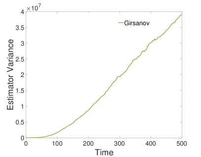
We begin by considering . Since is a parameter of the chemical model, we utilize Algorithm 2 for the Girsanov method and Algorithm 3 for the finite difference methods. For each method, we utilized 1,000 paths to estimate the derivative. For the finite difference methods, each “path” consists of a realization of the coupled processes (therefore, we end with 1,000 copies of each of and ). Moreover, we used a perturbation of .
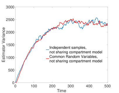
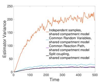
In Figure 1 we report the estimator variances
| (8) |
for the Girsanov and finite difference methods, respectively, where is the function that returns “Total S”, and is the weight function for the Girsanov method. We explicitly point out that the Split Coupling and the Common Reaction Path method have nearly identical estimator variances (as expected from [8]), and both are substantially lower than the other methods. We also note that, for the sake of comparison, we have provided two methods not detailed in the previous section: the use of independent samples and Common Random Variables that do not share the compartment model (making these the most naive methods possible). We do so to be able to visualize the benefit of coupling through the compartments, which is substantial.
While the Split Coupling and the Common Reaction Path method provide the lowest, and nearly identical, estimator variances, that does not mean they are equal in quality. As described in the previous section, this is because our implementation of the Common Reaction Path method is more like the “local” Common Reaction Path method of [8], in which the shared unit-rate Poisson processes are replaced between every compartment event. We provide in Table 1 the time required to generate these 1,000 paths (using the same computer under similar circumstances).
| Method | Time to generate 1,000 paths |
|---|---|
| Girsanov | 75 seconds |
| Independent samples, not sharing compartment model | 149 seconds |
| Common Random Variables, not sharing compartment model | 151 seconds |
| Independent samples, shared compartment model | 139 seconds |
| Common Random Variables, shared compartment model | 201 seconds |
| Common Reaction Path, shared compartment model | 426 seconds |
| Split Coupling, shared compartment model | 175 seconds |
A few notes are in order.
-
•
Because there is no coupling, the Girsanov method is expected to require at most one-half the simulation time of any other method. Note, however, that the faster simulation time is far outweighed by the high variance of the method.
-
•
The Common Reaction Path method takes significantly longer than any other method. This is due to the fact that we needed to pre-allocate the random vectors for the shared unit-rate Poisson processes for each reaction network, within each compartment, between each compartment event. Of course, part of the dramatic increase in simulation time could be due to either our implementation or the use of Matlab (as opposed to Python or C++). However, as there is always extra overhead with the method, it will always be slower than the Split Coupling method. Also, because of the results of [8], it will always have a similar variance to the split coupling method. Hence, we suggest it never be used.
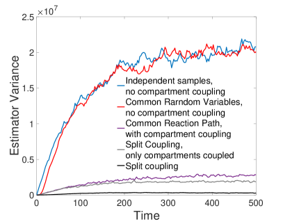
Now we turn to estimating . As is a parameter of the compartment model, there is no longer the possibility of sharing the compartment model. We once again simulated 1,000 paths of the processes, to time 500, while now using (which is, once again, one-tenth the value of the parameter). See Figure 2 for the estimator variances of the various methods. See Table 2 for the times required to generate the 1,000 paths for each method. We note that, once again, the Split Coupling method is the most efficient.
| Method | Time to generate 1,000 paths |
|---|---|
| Girsanov | 77 seconds |
| Independent samples, no compartment coupling | 148 seconds |
| Common Random Variables, no compartment coupling | 150 seconds |
| Common Reaction path, compartment coupling only | 176 seconds |
| Split Coupling, compartment and chemistry both coupled | 171 seconds |
| Split Coupling, compartment coupling only | 137 seconds |
Example 4.2 (Genetic model with coagulation).
Our second example has a chemistry that consists of transcription, translation, and dimerization of the resulting protein. This particular model is Example 2.4 in [10], and consists of the following set of reactions
| (9) | ||||
with and . We will assume that each cell/compartment has one gene, and so we suppress that species. Hence, this is a three species model with . For the compartment model, we have
, , , and . We will initialize the RNIC model with a single compartment with zero copies of each species. Moreover, we will initialize each compartment that appears with a reaction network with zero copies of each species. Finally, we will use our methods to estimate
where “Total dimers” is the sum of the number of dimers across all compartments.
See Figure 3 for the variances of the different methods when estimating .
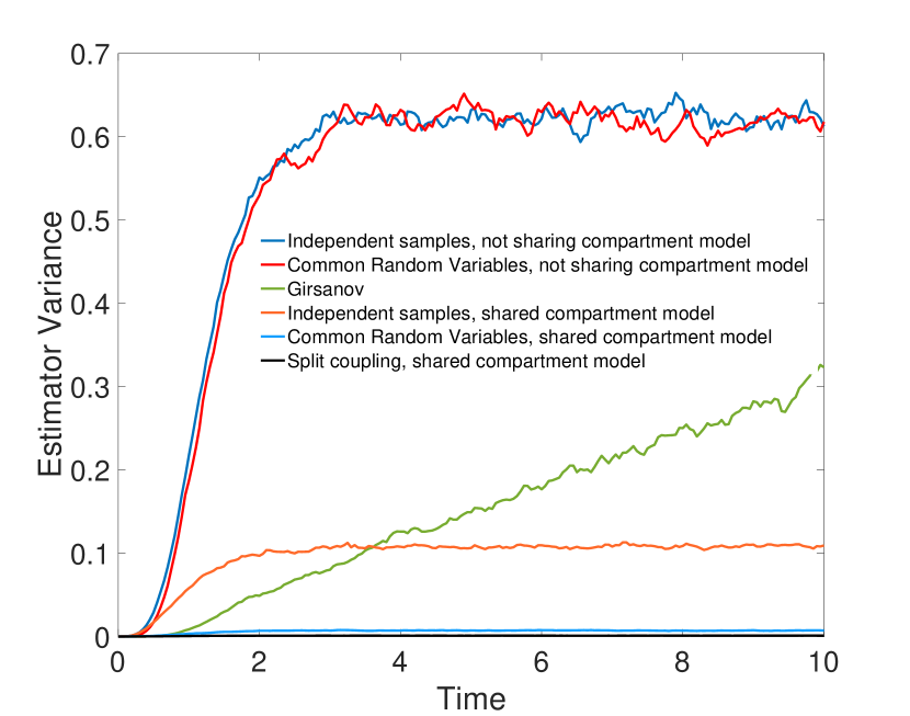
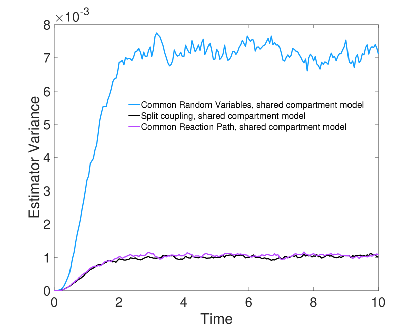
We note that, as expected, the simple act of sharing the compartment model provides the lion share of the variance reduction. We also note that the Split Coupling provides an estimator with such a low variance that it is difficult to differentiate from the -axis. We therefore zoom in and provide in Figure 4 a plot of the three methods with the lowest estimator variance. In each, the compartment model is shared between the coupled processes (as detailed in Algorithm 3). The chemical models are coupled in the following ways: Common Random Variables (CRV), Common Reaction Path (CRP), and the Split Coupling. As predicted by the work in [8], and as seen in the previous example, the CRP method and the Split Coupling method provide nearly identical variances. Finally, in Table 3, we provide the simulation time required required for the various methods. As in the previous example, the Split Coupling, with shared compartments, is clearly the most efficient.
| Method | Time to generate 10,000 paths |
|---|---|
| Girsanov | 344 seconds |
| Independent samples, not sharing compartment model | 720 seconds |
| Common Random Variables, not sharing compartment model | 747 seconds |
| Independent samples, shared compartment model | 662 seconds |
| Common Random Variables, shared compartment model | 1002 seconds |
| Common Reaction path, shared compartment model | 1080 seconds |
| Split Coupling, shared compartment model | 517 seconds |
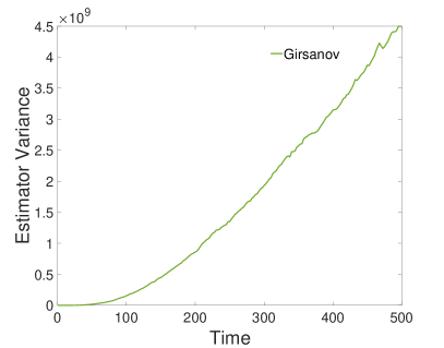
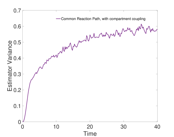
We turn to estimating . We once again simulatd 10,000 paths of the process, to time , while using . Figure 5 provides plots of the estimator variance for each method. We note that up through time 4, the Girsanov method has a lower variance than the split coupling method. However, as expected, the variance of the Girsanov method increases monotonically as time increases and quickly becomes significantly higher than the Split Coupling. We do not provide a table of simulation times, as they are similar to the case when was perturbed. As with the previous examples, we conclude that the Split Coupling is the most efficient estimator of the desired derivative.
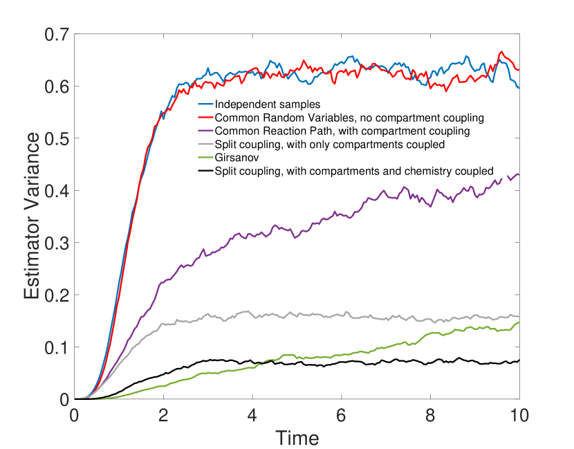
We note that the CRP method provides a variance that appears to be growing. This behavior is in line with the observations made in [3], where it was observed that the processes generated via the CRP method decouple as time increases, in which case the variance of the CRP method should approach that of independent samples. To confirm this behavior, we simulated the CRP method to time 40 and provide the relevant plot in Figure 6.
5 Discussion
In this paper, we have provided a comprehensive look at Monte Carlo methods for RNIC models, as introduced in [15, 6]. In particular, we have synthesized decades of work related to parameteric sensitivity analysis for stochastic reaction networks and succinctly developed each of the relevant methods for this new, and more complex, modeling choice.
In terms of guidance, it is clear that the Split Coupling method introduced here for RNIC models is the most efficient method and we recommend its use over the others. Of course, if an unbiased method is desired for any reason, or if the simulation time required is particularly short, then the Girsanov transformation method can be used.
The RNIC model introduced here is the most “basic” version of the model, however it can be generalized in number of ways. For example, it is possible to allow the transition rates of the compartment model (e.g., the fragmentation rate) to depend upon the contents of the compartments [15, 7]. More thought will need to be given as to how to implement the various methods in this case.
Appendix A Monte Carlo and finite difference methods for parametric sensitivities
The basic theory of Monte Carlo and finite difference methods for parametric sensitivities can be found in a multitude of papers and textbooks. The material presented here is added solely for completeness and is similar to that found in [3, Section 2.1].
Let be a family, parameterized by , of continuous-time stochastic processes with state space . In the setting of the current paper, is a continuous-time Markov chain with a discrete state space. We are assuming is one-dimensional here, but everything extends in the obvious manner if for some finite, positive integer .
Let be a function of the state of the system that gives a measurement of interest and define
The problem of interest is to efficiently estimate , and to do so using finite difference methods with Monte Carlo. (The other method utilized in this paper, a Girsanov or Likelihood Transformation method, is discussed in Section 3.1.)
In order to estimate , it is natural to utilize a centered finite difference:
| (10) |
as its bias is , as [12]. This should be compared with the forward difference, which has a bias of
The estimator for (10) using centered finite differences is
| (11) |
with
| (12) |
where represents the th path generated with parameter choice , is the number of paths generated, and the are generated independently.
Many computations are performed with a target variance (which yields a target size of the confidence interval). Denoting the target variance by , we see that the number of paths required is approximated by the solution to
Thus, decreasing the variance of lowers the computational complexity (total number of computations) required to solve the problem.
The basic idea of coupling is to lower the variance of by simulating and simultaneously, i.e., generating them on the same probability space, so that the two processes are highly correlated or “coupled.” That is, instead of generating paths independently, we want to generate a pair of paths so that the variance of is reduced. The basic idea of any such coupling is to reuse, or share, some portion of randomness in the generation of each process. The couplings utilized in this paper, found in Section 3, include using Common Random Variables (i.e., simply reusing the seed of the random number generator before generating each path), a version of the Common Reaction Path method [30], and a version of the Split Coupling [3].
Appendix B Standard algorithms for stochastic reaction networks
We provide the Gillespie algorithm [19, 20] and the next reaction method [18, 2], which are the two exact simulation methods that are most widely used. We also provide a Gillespie version of the Girsanov transformation method.
We remind that throughout this work, we assume a reaction network with reaction vectors denoted by , as in (1), and intensity functions (or rate functions) denoted by , where we have indexed the reactions by . For the sake of clarity, we will denote (in this section only) the number of reaction types by .
Algorithm 4 (Gillespie’s algorithm).
Given: a reaction network with reaction vectors and intensity functions , an initial distribution, , on .
Repeat steps 3 – 8 until a stopping criteria is reached. All calls to random variables are independent from all others.
-
1.
Determine via .
-
2.
Set .
-
3.
For each , determine and set .
-
4.
Let be independent random variables that are uniformly distributed on .
-
5.
Set .
-
6.
Find so that
-
7.
Set .
-
8.
Set .
We now provide the next reaction method, as it appeared in [2]. Note that this algorithm is simply a method for simulating Kurtz’s representation (2). Essentially the same algorithm (though with the addition of the usage of index priority queues) appeared in [18].
Algorithm 5 (Next Reaction method [2]).
Given: a reaction network with reaction vectors and intensity functions , an initial distribution, , on .
Repeat steps 5 – 10 until a stopping criteria is reached. All calls to random variables are independent from all others.
-
1.
Determine via .
-
2.
Set .
-
3.
For each , set .
-
4.
Let be a collection of independent unit-exponential random variables and for each , set .
-
5.
For each , determine .
-
6.
Find the minimum of the values . Denote the minimum by and denote the index of the minimum value by .
-
7.
Set .
-
8.
For each , set .
-
9.
Set , where is a unit-exponential random variable (independent from previous).
-
10.
Set .
We turn to the Girsanov transformation method, often called the Likelihood Transformation method outside of the biosciences. See either [28] or [12] for relevant references. For concreteness, we will assume stochastic mass-action kinetics and we suppose that we are computing the derivative of with respect to the rate parameter , where is some fixed time. We will denote the required weight function by . Therefore, the output of the algorithm consists of both and , which can be used as an unbiased estimator , where the subscript enumerates the independent realizations.
Algorithm 6 (Girsanov transformation method).
Given: a reaction network with reaction vectors and intensity functions , an initial distribution, , on .
All calls to random variables are independent from all others.
-
1.
Determine via .
-
2.
Set and .
-
3.
For each , determine and set .
-
4.
Let be independent random variables that are uniformly distributed on .
-
5.
Set .
-
6.
If , do the following (otherwise, proceed to step 7):
-
(a)
set
-
(b)
set ,
-
(c)
break from the algorithm and report and .
-
(a)
-
7.
Find so that
-
8.
If , set
otherwise, if , set
-
9.
Set .
-
10.
Set , and return to step 3.
Acknowledgement
This work was supported by a grant from the Simons Foundation (905083, Anderson). Anderson also gratefully acknowledges NSF grant support from DMS-2051498. Howells acknowledges support from the project “ConStRAINeD- Convergence and Stability of Reaction and Interaction Network Dynamics” funded by the MUR Progetti di Rilevante Interesse Nazionale (PRIN) - grant 2022XRWY7W.
References
- [1] Ikemefuna C. Agbanusi and Samuel A. Isaacson. A comparison of bimolecular reaction models for stochastic reaction–diffusion systems. Bulletin of mathematical biology, 76(4):922–946, 2014.
- [2] David F. Anderson. A modified Next Reaction Method for simulating chemical systems with time dependent propensities and delays. J. Chem. Phys., 127(21):214107, 2007.
- [3] David F. Anderson. An efficient finite difference method for parameter sensitivities of continuous time Markov chains. SIAM Journal on Numerical Analysis, 50(5):2237–2258, 2012.
- [4] David F. Anderson, Gheorghe Craciun, and Thomas G. Kurtz. Product-form stationary distributions for deficiency zero chemical reaction networks. Bull. Math. Biol., 72(8):1947–1970, 2010.
- [5] David F. Anderson and Desmond J Higham. Multi-level Monte Carlo for continuous time Markov chains, with applications in biochemical kinetics. SIAM: Multiscale Modeling and Simulation, 10(1):146–179, 2012.
- [6] David F. Anderson and Aidan S. Howells. Stochastic reaction networks within interacting compartments. Bulletin of Mathematical Biology, 85(10):87, 2023.
- [7] David F. Anderson, Aidan S. Howells, and Diego Rojas La Luz. Stochastic reaction networks within interacting compartments with content-dependent fragmentation. In progress, 2024.
- [8] David F. Anderson and Masanori Koyama. An asymptotic relationship between coupling methods for stochastically modeled population processes. IMA Journal of Numerical Analysis, 35(4):1757–1778, 2015.
- [9] David F. Anderson and Thomas G. Kurtz. Continuous time Markov chain models for chemical reaction networks. In H Koeppl Et al., editor, Design and Analysis of Biomolecular Circuits: Engineering Approaches to Systems and Synthetic Biology, pages 3–42. Springer, 2011.
- [10] David F. Anderson and Thomas G. Kurtz. Stochastic analysis of biochemical systems, volume 1.2 of Stochastics in Biological Systems. Springer International Publishing, Switzerland, 1 edition, 2015.
- [11] Adam P. Arkin, John Ross, and Harley H. McAdams. Stochastic kinetic analysis of developmental pathway bifurcation in phage lambda-infected Escherichia coli cells. Genetics, 149:1633–1648, 1998.
- [12] Søren Asmussen and Peter W. Glynn. Stochastic Simulation: Algorithms and Analysis. Stochastic modelling and applied probability. Springer, New York, 2007.
- [13] A Becskei, Benjamin B. Kaufmann, and A Van Oudenaarden. Contributions of low molecule number and chromosomal positioning to stochastic gene expression. Nature Genetics, 37(9):937–944, 2005.
- [14] Masao Doi. Stochastic theory of diffusion-controlled reaction. Journal of Physics A: Mathematical and General, 9(9):1479, 1976.
- [15] Lorenzo Duso and Christoph Zechner. Stochastic reaction networks in dynamic compartment populations. Proceedings of the National Academy of Sciences, 117(37):22674–22683, 2020.
- [16] Michael B. Elowitz, Arnold J. Levin, Eric D. Siggia, and Peter S. Swain. Stochastic Gene Expression in a Single Cell. Science, 297(5584):1183–1186, 2002.
- [17] Radek Erban and Hans G. Othmer. Special issue on stochastic modelling of reaction–diffusion processes in biology, 2014.
- [18] Michael A. Gibson and Jehoshua Bruck. Efficient exact stochastic simulation of chemical systems with many species and many channels. J. Phys. Chem. A, 105:1876–1889, 2000.
- [19] Daniel T. Gillespie. A general method for numerically simulating the stochastic time evolution of coupled chemical reactions. J. Comput. Phys., 22:403–434, 1976.
- [20] Daniel T. Gillespie. Exact Stochastic Simulation of Coupled Chemical Reactions. J. Phys. Chem., 81(25):2340–2361, 1977.
- [21] Paul Glasserman. Gradient estimation via perturbation analysis, volume 116. Springer Science & Business Media, 1990.
- [22] D. Huh and Johan Paulsson. Non-genetic heterogeneity from stochastic partitioning at cell division. J. Nat. Genet., 43(2):95–100, 2011.
- [23] Samuel A. Isaacson. A convergent reaction-diffusion master equation. The Journal of Chemical Physics, 139(5), 2013.
- [24] Michal Komorowski, Maria J. Costa, David A. Rand, and Michael P. H. Stumpf. Sensitivity, robustness, and identifiability in stochastic chemical kinetics models. PNAS, 108(21):8645–8650, 2011.
- [25] Thomas G. Kurtz. Strong approximation theorems for density dependent Markov chains. Stoch. Proc. Appl., 6:223–240, 1978.
- [26] Hédia Maamar, Arjun Raj, and David Dubnau. Noise in Gene Expression Determines Cell Fate in Bacillus subtilis. Science, 317(5837):526–529, 2007.
- [27] Johan Paulsson. Summing up the noise in gene networks. Nature, 427:415–418, 2004.
- [28] Sergey Plyasunov and Adam P. Arkin. Efficient stochastic sensitivity analysis of discrete event systems. J. Comp. Phys., 221:724–738, 2007.
- [29] J. M. Raser and E. K. O’Shea. Control of Stochasticity in Eukaryotic Gene Expression. Science, 304:1811–1814, 2004.
- [30] Muruhan Rathinam, Patrick W. Sheppard, and Mustafa Khammash. Efficient computation of parameter sensitivities of discrete stochastic chemical reaction networks. Journal of Chemical Physics, 132:34103, 2010.
- [31] Steffen Rulands, Fabienne Lescroart, Samira Chabab, Christopher J. Hindley, Nicole Prior, Magdalena K. Sznurkowska, Meritxell Huch, Anna Philpott, Cedric Blanpain, and Benjamin D. Simons. Universality of clone dynamics during tissue development. Nature physics, 14(5):469–474, 2018.
- [32] Timothy E. Saunders. Aggregation-fragmentation model of robust concentration gradient formation. Physical Review E, 91(2):022704, 2015.
- [33] R. Srivastava, L. You, J. Summers, and J. Yin. Stochastic vs. Deterministic Modeling of Intracellular Viral Kinetics. J. Theor. Biol, 218:309–321, 2002.
- [34] S. Uphoff, N. D. Lord, L. Potvin-Trottier, B. Okumus, D. J. Sherratt, and J. Paulsson. Stochastic activation of a DNA damage response causes cell-to-cell mutation rate variation. Science, 351(6277):1094–1097, 2016.
- [35] Quentin Vagne and Pierre Sens. Stochastic model of maturation and vesicular exchange in cellular organelles. Biophysical Journal, 114(4):947–957, 2018.
- [36] Elizabeth Skubak Wolf and David F. Anderson. Hybrid pathwise sensitivity methods for discrete stochastic models of chemical reaction systems. The Journal of Chemical Physics, 142(3), 2015.