DRL-Based Resource Allocation for Motion Blur Resistant Federated Self-Supervised Learning in IoV

Abstract

In the Internet of Vehicles (IoV), Federated Learning (FL) provides a privacy-preserving solution by aggregating local models without sharing data. Traditional supervised learning requires image data with labels, but data labeling involves significant manual effort. Federated Self-Supervised Learning (FSSL) utilizes Self-Supervised Learning (SSL) for local training in FL, eliminating the need for labels while protecting privacy. Compared to other SSL methods, Momentum Contrast (MoCo) reduces the demand for computing resources and storage space by creating a dictionary. However, using MoCo in FSSL requires uploading the local dictionary from vehicles to Base Station (BS), which poses a risk of privacy leakage. Simplified Contrast (SimCo) addresses the privacy leakage issue in MoCo-based FSSL by using dual temperature instead of a dictionary to control sample distribution. Additionally, considering the negative impact of motion blur on model aggregation, and based on SimCo, we propose a motion blur-resistant FSSL method, referred to as BFSSL. Furthermore, we address energy consumption and delay in the BFSSL process by proposing a Deep Reinforcement Learning (DRL)-based resource allocation scheme, called DRL-BFSSL. In this scheme, BS allocates the Central Processing Unit (CPU) frequency and transmission power of vehicles to minimize energy consumption and latency, while aggregating received models based on the motion blur level. Simulation results validate the effectiveness of our proposed aggregation and resource allocation methods.

I Introduction

Internet of Vehicles (IoV) is a technology that connects vehicles, road and transportation facilities to Internet, enabling intelligent interaction and information sharing among them. Advances in IoV have made many practical applications possible, e.g., automatic navigation, meteorological information and road condition monitoring, which provide convenience to drivers and self-driving system, reduce the probability of accidents and improve the efficiency of the transportation system [1]-[3]. These applications need robust models, which require a lot of data for training. In IoV, vehicles can continuously capture the fresh data along the moving road, including road conditions and environmental states through onboard sensors, where most of the data are captured in the form of images [4]-[6]. Moreover, vehicles also can store the image data locally and deal with them to realize recognition and classification, which provides essential information for self-driving and driver assistance systems to aid drivers in perceiving and understanding surroundings.

However, the locally stored image data, denoted as local data, is usually private for vehicles, and vehicles are reluctant to share the data with each other to protect privacy. Since vehicles come from all directions, the local data they collect vary greatly. If the model, denoted as local model, is trained locally based on the local data, it may converge to a local optimum [7]-[9]. In contrast to distributed training, Federated Learning (FL) performs a centered training and enables a Base Station (BS) to obtain a global model through aggregating local models from vehicles without sharing the local data, thereby providing a privacy-preserving solution and reducing the differences between local models [10][11]. For local training, the traditional supervised learning requires the image data with labels [12]-[14], but data labeling requires significant manual effort. Especially in IoV, a large amount of unlabeled data is generated daily, further increasing the cost of manual labeling. The Self-Supervised Learning (SSL) leverages pretext to provide training based on the inherent properties of data, thus it can learn feature representations from the data itself without the need for manually annotated labels. The traditional SSL methods obtain a better training performance through generating and storing abundant negative samples, which occupies a lot of computing resource and storage space. Thus, traditional methods are not suitable for the resource and space limited IoV. The famous SSL method Momentum Contrast (MoCo) uses $k$ values to form a dictionary and stand for the reference of negative samples, which can save computing resource and storage space [15][16]. However, employing MoCo in FSSL for local training will upload $k$ values to create a big dictionary in BS for aggregation, which may cause privacy leakage [17]-[19]. Moreover, the training performance of FSSL in IoV may be deteriorated due to the motion blur. Specifically, excessive vehicle velocity may result in insufficient exposure time of the camera sensor, causing image blur [20][21]. The blur level of images directly impacts the accuracy and convergence of the global model. To the best of our knowledge, there is no work considering the privacy leakage and motion blur for FSSL in IoV.

The improved MoCo method Simplified Contrast (SimCo) uses dual temperature to control sample distribution to eliminate the usage of dictionary [22]-[24], thus it can greatly protect privacy and is suitable for the local training of FSSL in IoV. Considering the negative impact of motion blur on model aggregation, we also propose a motion Blur resistant FSSL, refer to as BFSSL.

It is noteworthy that increasing Central Processing Unit (CPU) frequency of a vehicle results in more local training iterations while consuming more energy consumption. Higher transmission power of a vehicle reduces the transmission delay, while costing more energy. Simultaneously, low CPU frequency reduces the number of local iterations within the given processing period of time, thereby diminishing the accuracy of the global model [25][26]. Additionally, low transmission power increases data interference, resulting in higher rates of transmission failure. Thus, it is critical to find a resource allocation scheme that allocates resources (i.e., CPU frequency and transmission power of vehicles) to minimize energy consumption and delay for the BFSSL, while increasing the success rate of transmission in IoV. Since the resource allocation problem is usually non-convex in the complicated IoV, the traditional convex optimization methods are difficult to solve it. Deep Reinforcement Learning (DRL) is a good option to solve the non-convex problem. In this paper, we propose the DRL-BFSSL algorithm, where vehicles employs SimCo to perform locally training and sends local models to BS for blur-based aggregation. Meanwhile, BS allocates CPU frequency and transmission power to minimize the energy consumption and delay.

Overall, the main contributions of this paper can be summarized as follows:

• Based on the concept of FL, we enable vehicles to perform SimCo locally with their own unlabeled image data. This approach not only effectively safeguards the privacy of vehicles but also avoids labeled data.

• In IoV, we utilize the level of motion blur as a crucial weighting factor on Independent and Identically Distributed (IID) and Non-IID datasets during model aggregation. Subsequently, by aggregating models uploaded by training vehicles associated with the blur level, we obtain a blur resistant global model.

• We firstly formulate an optimization problem aiming to minimize the sum of energy consumption and delay. Subsequently, utilizing the Karush-Kuhn-Tucker (KKT) conditions to determine the optimal solution that jointly allocating bandwidth and CPU frequency. Finally, by the Soft Actor-Critic (SAC) algorithm, we identify the optimal allocation schedule for the CPU frequency and transmission power of each vehicle. Meanwhile, considering that low transmission power may lead to data transmission failures, we use the data error rate to set a minimum transmission power limit.

The rest of this paper is divided into several interrelated parts to comprehensively explore the discussed problem. In Section II, we will review prior work relevant to this study, providing background and context for subsequent discussions. In Section III, we describe the system model. In Section IV, we will formulate an optimization problem aiming to minimize the sum of energy consumption and delay and in Section V, we will introduce our proposed DRL-BFSSL algorithm. Section VI showcase and discuss the simulation results. Ultimately, we will summarize the paper in Section VII.

II Related Work

In this section, we will introduce the related work about FSSL and resource allocation based on DRL in IoV.

II-A Federated SSL

In [27], Jahan et al. proposed a FSSL which combines FL and the SSL method (i.e., Simple framework for Contrastive Learning of Representations (SimCLR)), to identify Mpox from skin lesion images [28]. In [29], Yan et al. proposed a FSSL which combines FL and the SSL method (i.e., Variational inference with adversarial learning for end-to-end text-to-speech (Vits)), and utilizes medical images stored in each hospital to train models. In [30], Xiao et al. proposed a FSSL which integrates Generative Adversarial Networks (GAN) as a pretext for SSL and combines it with FL to support automatic traffic analysis and synthesis over a large number of heterogeneous datasets. In [31], Li et al. proposed a FSSL which integrates You Only Look Once (YOLO) as a pretext for SSL and combines it with FL to process object detection in power operation sites. These FSSL methods mentioned above require a large number of samples for training, which imposes high demands on the computing and storage capabilities of devices. However, the computing and storage resources of vehicles are limited in IoV, thus these methods are not suitable for IoV.

To mitigate the demand on computing and storage capabilities, some methods have been introduced accordingly. In [32], Feng et al. applied FL to enhance the performance of Acoustic Event Classification (AEC) and improve downstream AEC classifiers by performing SSL with small negative samples locally without labels for saving computing and storage resources, and adjusting model parameters globally with labels. However, this method does not fully leverage the advantage of SSL learning without labels. In [33], instead of employing all the negative samples, Shi et al. proposed a SSL method to automatically select a core set of most representative samples on each device and store them in a replay buffer for saving computing and storage capabilities of devices. In [34], Wei et al. combined FL and MoCo to propose a FSSL named Federated learning with momentum Contrast (FedCo) for IoV, where MoCo is a special SSL method which employs dictionary to provide the reference of negative samples, which can save computing resource and storage space [35]. However, for FedCo, vehicles uploaded local $k$ values for forming a new big dictionary in global side, which fails to ensure privacy protection and goes against the original intention of using FL. In [22], Zhang et al. proposed the SSL method SimCo base on MoCo, and utilized dual temperatures to control sample distribution, thus SimCo not only saves computing resource and storage space but also protects privacy. To the best of our knowledge, there is no related work proposed a FSSL based on SimCo to reduce computing resource and storage space while protecting privacy in IoV. Furthermore, the training performance of FSSL in IoV may be deteriorated due to the motion blur, and there is no related work that considers motion blur in the related works that employs FSSL in IoV. Hence, we consider the motion blur and propose a FSSL based SimCo for IoV to resist motion blur, referred as to BFSSL.

II-B DRL-based resource allocation scheme in FL

Some works have proposed DRL-based resource allocation schemes in IoV. In [36], Zheng et al. proposed a resource allocation scheme based on DRL method to minimize the duration required for accomplishing tasks while respecting latency limitations in IoV. In [37], Hazarika et al. proposed a resource allocation scheme based on DRL method to allocate the power optimally in IoV. In [38], Guo et al. proposed a resource allocation scheme based on DRL method to minimize the cost of Road Side Unit (RSU) in IoV. However, the methods mentioned above have not considered the FL framework. There are also some works that consider the FL framework to address resource allocation problems based on DRL. In [39], He et al. combined FL and DRL method (i.e., Deep Deterministic Policy Gradient (DDPG)), to optimize both computation offloading and resource allocation. In [40], Zhang et al. combined FL and DRL method (i.e., DDPG), and proposed a dynamic computation offloading and resource allocation scheme to minimize the delay and energy consumption.

However, there is no work concerning the DRL-based resource allocation schemes for FSSL in IoV. Therefore, we further investigate a DRL-based resource allocation scheme to optimize the performance for the BFSSL in IoV, referred to as DRL-BFSSL.

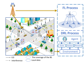
Figure 1: System scenario

III System Model

In this section, we will introduce the system scenario and models. As shown in Fig. 1, we consider a scenario of a BS deployed at the center of the intersection and several vehicles driving in the coverage of the BS. When a vehicle arrives at the intersection, it turns left, turns right and drives straightly with probabilities $\varepsilon_{1}$, $\varepsilon_{2}$, $\varepsilon_{3}$, and $\varepsilon_{1}+\varepsilon_{2}+\varepsilon_{3}=1$, and then it keeps driving straightly. Vehicle velocity follows the truncated Gaussian distribution. Each vehicle is equipped with a camera to capture images during driving through the coverage area of the BS, and the vehicles coming from different directions capture different categories of images. $N$ training vehicles are randomly selected from the vehicles before crossing the intersection to ensure that vehicles have enough time for local training. Vehicle $n$, $n\in[1,N]$, is equipped with a camera and captures $Z$ image data with velocity $v_{0}^{n}$ before it enters the coverage area of the BS.

The entire process of DRL-BFSSL algorithm consists of $K^{\text{max}}$ episodes, each of which is divided into two task lines, one for BFSSL, where episode $k$ is divided into different rounds, and the other for DRL-based resource allocation, where episode $k$ is divided into different slots[41][42].

Specifically, as shown in Fig. 2, within each episode $k$, $k\in[1,K^{\text{max}}]$ , there are $S^{\text{max}}$ slots, and each round $r$ corresponds to one slot. The difference is that at the end of each episode $k$, when entering the next episode $k+1$, slot $t$ is reset to slot $0$. In contrast, round $r$ is not reset and continues to accumulate until the whole process of DRL-BFSSL algorithm finished. Due to each episode containing $S^{\text{max}}$ slots, and round $r$ resets to 0 after the completion of the $K^{\text{max}}$ episodes, the relationship between slot $t$ in episode $k$ and round $r$ is as follows

$$r=\left(k-1\right)S^{\text{max}}+t.$$ (1)

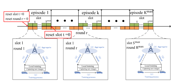
Figure 2: The process of DRL-BFSSL algorithm

At the beginning of the DRL-BFSSL algorithm, the BS collects the initial positions of training vehicles and initializes a global model. For the task line of BFSSL, at the beginning of each round $r$, BS uses the model aggregated at the end of round $r-1$ as the global model for round $r$. Meanwhile, for the task line of resource allocation, at the beginning of each slot $t$, the BS receives the velocities uploaded by vehicles and estimate the positions based on the initial positions and received velocities, after that it adopts the DRL method to allocate resources for training vehicles including transmission power and CPU frequency. Then each training vehicle downloads the global model from the BS, along with the allocated transmission power and CPU frequency. After that each vehicle trains locally based on the global model to update its local model. In this process, each vehicle firstly randomly chooses a certain number of images from captured images as local data and subsequently conducts local training through iterations to update the local model. During the process of local training, the vehicles also capture new images for the training of next round. When the local training is finished, each vehicle adopts the downloaded transmission power to transmit its updated local model and velocity to BS. However, during the transmission process, varying signals transmitted by other vehicles may cause interference, leading to data errors that prevent the BS from receiving the uploaded local models. Finally, BS aggregates the received local models to obtain a new global model based on the motion blur. The above process is repeated in different episode to get a converged global model.

In the following, we will introduce the mobility model, transmission model, computing model, and data error model in slot $t$ of each episode $k$.

III-A Mobility model

As the velocity of each vehicle $n$ follows the truncated Gaussian distribution to reflect real vehicle mobility, the velocities of different vehicles are IID. Let $v_{k,t}^{n}$ be the velocity of vehicle $n$, and $v^{\text{min}}$ and $v^{\text{max}}$ be the minimum and maximum velocity of vehicles, respectively. Thus the probability density function of $v_{k,t}^{n}$ is calculated as [43]-[45]

$$\vspace{-0.25cm}f\left(v_{k,t}^{n}\right)=\left\{\begin{aligned} \frac{{{e^{-\frac{1}{{2{\sigma^{2}}}}{{({v_{k,t}^{n}}-\mu)}^{2}}}}}}{{\sqrt{2\pi{\sigma^{2}}}[\text{erf}(\frac{{{v^{\max}}-\mu}}{{\sigma\sqrt{2}}})-\text{erf}(\frac{{{v^{\min}}-\mu}}{{\sigma\sqrt{2}}})]}}\\ {v^{\text{min}}}\leq{v_{k,t}^{n}}\leq{v^{\text{max}}}\\ 0\qquad\qquad\qquad\qquad\quad\text{otherwise}\end{aligned}\right.,$$ (2)

where $\text{erf}(\mu,\sigma^{2})$ is the Gaussian error function of velocity $v_{k,t}^{n}$ with mean $\mu$ and variance $\sigma^{2}$.

III-B Transmission model

During the transmission process, the energy consumption of vehicle $n$ can be calculated as [46][47]

$$E_{k,t}^{{\text{trans}},n}=p_{k,t}^{n}T_{k,t}^{{\text{trans}},n},$$ (3)

where $p_{k,t}^{n}$ is the transmission power of vehicle $n$, $T_{k,t}^{{\text{trans}},n}$ is the transmission delay required by vehicle $n$ to transmit local model. We consider that each vehicle transmits a local model with the the same size $Z$, thus $T_{k,t}^{{\text{trans}},n}$ can be calculated as

$$T_{k,t}^{{\text{trans}},n}=\frac{Z}{c_{k,t}^{n}},$$ (4)

where $c_{k,t}^{n}$ is the transmission rate of vehicle $n$, which can be calculated according to Shannon’s theorem [48]-[50], i.e.,

$$c_{k,t}^{n}=\beta_{k,t}^{n}B^{U}\text{ln}\left(1+\frac{p_{k,t}^{n}h_{k,t}^{n}}{I_{k,t}^{n}+B^{U}N_{0}}\right),$$ (5)

where $\beta_{k,t}^{n}$ is the proportion of the bandwidth allocated to vehicle $n$, $B^{U}$ is the uplink bandwidth, $I_{k,t}^{n}$ is interference and $N_{0}$ is the noise power. $h_{k,t}^{n}$ is the channel power gain between vehicle $n$ and the BS, which is calculated as [51]:

$$h_{k,t}^{n}=g_{n}\varrho_{n}\mathcal{A}\left(L_{k,t}^{n}\right)^{-\iota},$$ (6)

where $g_{n}$ represents the small-scale fast fading power, which follows an exponential distribution with unit mean. $\varrho_{n}$ represents shadow fading with a standard deviation of $\xi$. $\mathcal{A}$ is the path loss constant, $L_{k,t}^{n}$ is the distance between vehicle $n$ and BS, and $\iota$ is the decay exponent.

III-C Computing model

During the local training, the energy consumption of vehicle $n$ to execute each iteration of local training is calculated as

$$E_{k,t}^{{\text{comp}},n}=p_{k,t}^{{\text{comp}},n}T_{k,t}^{{\text{comp}},n},$$ (7)

where $T_{k,t}^{{\text{comp}},n}$ is the computing delay of vehicle $n$ to execute one iteration of local training, and $p_{k,t}^{{\text{comp}},n}$ is the CPU computing power of vehicle $n$, that can be calculated by Dynamic Voltage Frequency Scaling (DVFS) approach [52]-[54], i.e.,

$$p_{k,t}^{{\text{comp}},n}=\kappa\left(f_{k,t}^{n}\right)^{3},$$ (8)

where $\kappa$ is the effective switched capacitance, which depends on the chip architecture, and $f_{k,t}^{n}$ is the CPU frequency allocated to vehicle $n$ for computation. Let $f^{\text{min}}$ and $f^{\text{max}}$ be the minimum and maximum CPU computation frequency, thus $f_{k,t}^{n}\in[f^{\text{min}},\ f^{\text{max}}]$.

Let $r_{\text{cyc}}$ be the number of CPU cycles for processing the unit size and $D_{\text{data}}$ be the local data size. $|D_{\text{data}}|r_{\text{cyc}}$ represents the required CPU cycles in local training. Hence, the computing delay $T_{k,t}^{{\text{comp}},n}$ is calculated as

$$T_{k,t}^{{\text{comp}},n}=\frac{\left|D_{\text{data}}\right|r_{\text{cyc}}}{f_{k,t}^{n}}.$$ (9)

Substituting Eqs. (8) and (9) into Eq. (7) , we can obtain

$$E_{k,t}^{{\text{comp}},n}=\kappa\left(f_{k,t}^{n}\right)^{2}\left|D_{\text{data}}\right|r_{\text{cyc}}.$$ (10)

III-D Data error model

In data transmission, both the variations signals transmitted by other vehicles may cause interference that incurs an error probability for the data of the local model received by the BS. Cyclic Redundancy Check (CRC) mechanism is employed here to describe error for the data of local model received by the BS [55]. According to the CRC mechanism, the data error probability $\epsilon_{k,t}^{n}$ for vehicle $n$ in slot $t$ of episode $k$ is calculated as[56]

$$\epsilon_{k,t}^{n}\left(p_{k,t}^{n}\right)=1-\text{exp}\left[-\frac{m\left(I_{k,t}^{n}+B^{U}N_{0}\right)}{p_{k,t}^{n}h_{k,t}^{n}}\right],$$ (11)

where $m$ is a waterfall threshold. Let $C_{k,t}^{n}(p_{k,t}^{n})$ indicates if the BS successfully received the uploaded model with respect to $p_{k,t}^{n}$. Thus we have

$$\vspace{-0.00cm}C_{k,t}^{n}(p_{k,t}^{n})=\begin{cases}1,&\text{with probability }(1-\epsilon_{k,t}^{n})\\ 0,&\text{with probability }\epsilon_{k,t}^{n}\end{cases}.$$ (12)

IV Optimization Problem

The duration of one round is donated as $T$, which is divided into two phases: local training phase and uploading phase.

In the local training phase, higher CPU frequency allows for more iterations, which can enhance model performance but also increase energy consumption. In the uploading phase, vehicles upload the trained local model to BS. Higher transmission power reduces the upload time but increases energy consumption [57][58]. To save resources, we need to optimize the allocation of vehicle CPU frequencies and transmission power to minimize the overall energy consumption of all vehicles.

However, if the CPU frequency is too low, the time for a single local training iteration increases, resulting in fewer local iterations. Although this reduces energy consumption, it does not ensure the model’s performance [59][60]. Therefore, we also need to minimize the time for each training to ensure sufficient local iterations.

To deal with these two problems, our target is adjusted to minimize the total energy consumption of all vehicles and the max delay including model training and model transmission. The energy and delay for system performance can be calculated as:

$$E_{k,t}^{{\text{total}},n}=E_{k,t}^{{\text{trans}},n}+\left\lfloor N_{k,t}^{n}\right\rfloor E_{k,t}^{{\text{comp}},n},$$ (13)

$$T_{k,t}^{{\text{total}},n}=T_{k,t}^{{\text{trans}},n}+T_{k,t}^{{\text{comp}},n},$$ (14)

where$\left\lfloor N_{k,t}^{n}\right\rfloor$ is the number of iterations for local training, $\left\lfloor\cdot\right\rfloor$ represents the rounding down function. Since the number of iterations for local training should be a integer, the integral number of iterations $\left\lfloor N_{k,t}^{n}\right\rfloor$ can be calculated as

$$\left\lfloor N_{k,t}^{n}\right\rfloor=\left\lfloor\frac{T-t_{\max}^{\text{Trans}}}{T_{k,t}^{{\text{comp}},n}}\right\rfloor,$$ (15)

where $t_{\max}^{\text{Trans}}$ denotes the maximum allowable transmission delay. For a fixed $T$, $\left(T-t_{\max}^{\text{Trans}}\right)$ is the time used for local training. For simplicity, we use $\mathcal{N}_{k,t}^{n}$ to approximate the value $\left\lfloor N_{k,t}^{n}\right\rfloor$, where

$$\mathcal{N}_{k,t}^{n}=N_{k,t}^{n}-1.$$ (16)

Thus Eq. (13) can be expressed as

$$\begin{split}E_{k,t}^{{\text{total}},n}=E_{k,t}^{{\text{trans}},n}&+\mathcal{N}_{k,t}^{n}E_{k,t}^{{\text{comp}},n},\\ &\left\lfloor N_{k,t}^{n}\right\rfloor-1\leq{\mathcal{N}_{k,t}^{n}}\leq\left\lfloor N_{k,t}^{n}\right\rfloor.\end{split}$$ (17)

Let $\boldsymbol{\beta}=\left\{\beta_{k,t}^{1},\beta_{k,t}^{2},\cdots,\beta_{k,t}^{n},\cdots,\beta_{k,t}^{N}\right\}$,

$\boldsymbol{p}=\left\{{p_{k,t}^{1},p_{k,t}^{2},\cdots,p_{k,t}^{n},\cdots,p_{k,t}^{N}}\right\}$, and $\boldsymbol{f}=\left\{f_{k,t}^{1},f_{k,t}^{2},\cdots,f_{k,t}^{n},\cdots,f_{k,t}^{N}\right\}$ represent the sets of the allocated bandwidth ratios, transmission powers, and CPU frequencies, respectively. The optimization problem can be formulated as

$$\underset{\boldsymbol{\beta},\boldsymbol{p},\boldsymbol{f}}{\min}\mathcal{C}:\lambda_{1}\sum_{n=1}^{N}{E_{k,t}^{{\text{total}},n}+\lambda_{2}\max{T_{k,t}^{{\text{total}},n}}}\\$$ (18)

s.t.

$$0<\beta_{k,t}^{n}<1$$ (18a)

$$\sum_{n=1}^{N}\beta_{k,t}^{n}\leq 1$$ (18b)

$$\epsilon_{k,t}^{n}\leq\epsilon_{\tau}$$ (18c)

$$p^{\text{min}}\leq p_{k,t}^{n}\leq p^{\text{max}}$$ (18d)

$$f^{\text{min}}\leq f_{k,t}^{n}\leq f^{\text{max}}$$ (18e)

where $\lambda_{1}$ and $\lambda_{2}$ represent the weights assigned to the energy consumption and delay, respectively, thus $\lambda_{1},\ \lambda_{2}\in[0,1]$, and $\lambda_{1}+\lambda_{2}=1$. Eqs. (18a) and (18b) show that the allocated bandwidth for each vehicle $n$ maintains a reasonable range. Eq. (18c) ensures that the data error rate of vehicle $n$ is less than a specified value $\epsilon_{\tau}$. Eq. (18d) limits the minimum and maximum transmission power for each vehicle $n$, i.e., $p^{\text{min}}$ and $p^{\text{max}}$. Eq. (18e) limits the minimum and maximum CPU frequency for vehicle $n$, i.e., $f^{\text{min}}$ and $f^{\text{max}}$.

As can be seen from the above optimization problem, the restrictions Eqs. (18a) - (18e) increase the complexity of calculation and the difficulty of problem solving. Next we will simplify the restrictions.

Substituting Eqs. (13), (14) and (16) into Eq. (18), the optimization problem can be written as

$$\mathcal{C}=\lambda_{1}\sum_{n=1}^{N}E_{k,t}^{{\text{total}},n}+\lambda_{2}\max{T_{k,t}^{{\text{total}},n}}$$ (20)

$$=\sum_{n=1}^{N}\Big{[}\frac{\lambda_{1}p_{k,t}^{n}Z}{\beta_{k,t}^{n}B^{U}\ln\left(1+\frac{p_{k,t}^{n}h_{k,t}^{n}}{I_{k,t}^{n}+B^{U}N_{0}}\right)}$$

$$+\lambda_{1}\left(T-t_{\max}^{\text{Trans}}\right)\kappa\left(f_{k,t}^{n}\right)^{3}-\lambda_{1}\kappa\left(f_{k,t}^{n}\right)^{2}|D_{\text{data}}|r_{\text{cyc}}\Big{]}$$

$$+\max\Big{[}\frac{\lambda_{2}Z}{\beta_{k,t}^{n}B^{U}\ln\left(1+\frac{p_{k,t}^{n}h_{k,t}^{n}}{I_{k,t}^{n}+B^{U}N_{0}}\right)}+\frac{\lambda_{2}|D_{\text{data}}|r_{\text{cyc}}}{f_{k,t}^{n}}\Big{]}.$$

As shown in Eq. (20), the optimization problem involves multiple variables. To simplify the solving process, we introduce the following notations

$$A=\frac{\lambda_{1}p_{k,t}^{n}Z}{B^{U}\text{ln}\left(1+\frac{p_{k,t}^{n}h_{k,t}^{n}}{I_{k,t}^{n}+B^{U}N_{0}}\right)},$$ (21)

$$B=\lambda_{1}\kappa\left(T-t_{\max}^{\text{Trans}}\right),$$ (22)

$$C=\lambda_{1}\kappa\left|D_{\text{data}}\right|r_{\text{cyc}},$$ (23)

$$E=\frac{\lambda_{2}Z}{B^{U}\text{ln}\left(1+\frac{p_{k,t}^{n}h_{k,t}^{n}}{I_{k,t}^{n}+B^{U}N_{0}}\right)},$$ (24)

$$F=\lambda_{2}\left|D_{\text{data}}\right|r_{\text{cyc}},$$ (25)

where $A$, $B$, $C$, $E$, and $F$ depend on the parameter $p_{k,t}^{n}$ and the constant parameters related to the vehicle’s own configuration. Thus the optimization problem $\mathcal{C}$ is written as

$$\begin{split}\mathcal{C}=&\sum_{n=1}^{N}\left[\frac{A}{\beta_{k,t}^{n}}+B\left({f_{k,t}^{n}}\right)^{3}-C\left({f_{k,t}^{n}}\right)^{2}\right]\\ &+\max{\left(\frac{E}{\beta_{k,t}^{n}}+\frac{F}{f_{k,t}^{n}}\right)}.\end{split}$$ (26)

Then we utilize the KKT conditions to reduce the restrictions (18a) and (18b), while the detailed procedures is given in Appendix A. Thus we can obtain the relationship between $\beta_{k,t}^{n}$ and the introduced notations, i.e.,

$$\beta_{k,t}^{n}=\frac{\left[A+\frac{3B\left({f_{k,t}^{n}}\right)^{4}-2C\left({f_{k,t}^{n}}\right)^{3}}{F}E\right]^{\frac{1}{2}}}{\sum_{n=1}^{N}\left[A+\frac{3B\left({f_{k,t}^{n}}\right)^{4}-2C\left({f_{k,t}^{n}}\right)^{3}}{F}E\right]^{\frac{1}{2}}}.$$ (27)

According to the Eq. (11) and restriction (18c), we can establish the relationship between $\epsilon_{\tau}$ and $p_{k,t}^{n}$, thus Eq. (11) can be written as

$$p_{k,t}^{n}\geq\frac{-m\left(I_{k,t}^{n}+B^{U}N_{0}\right)}{h_{k,t}^{n}\text{ln}\left(1-\epsilon_{\tau}\right)}.$$ (28)

We define the right-hand side of Eq. (28) as $P^{\tau}$. Thus, the optimization problem $\mathcal{C}$ can be formulated as:

$$\begin{split}\underset{\boldsymbol{p},\boldsymbol{f}}{\min}\mathcal{C}:&\sum_{n=1}^{N}\Bigg{\{}\frac{A{\sum_{n=1}^{N}\left[A+\frac{3B\left({f_{k,t}^{n}}\right)^{4}-2C\left({f_{k,t}^{n}}\right)^{3}}{F}E\right]^{\frac{1}{2}}}}{\left[A+\frac{3B\left({f_{k,t}^{n}}\right)^{4}-2C\left({f_{k,t}^{n}}\right)^{3}}{F}E\right]^{\frac{1}{2}}}\\ &+B\left({f_{k,t}^{n}}\right)^{3}-C\left({f_{k,t}^{n}}\right)^{2}\Bigg{\}}\\ &+\max\Bigg{\{}\frac{E{\sum_{n=1}^{N}\left[A+\frac{3B\left({f_{k,t}^{n}}\right)^{4}-2C\left({f_{k,t}^{n}}\right)^{3}}{F}E\right]^{\frac{1}{2}}}}{\left[A+\frac{3B\left({f_{k,t}^{n}}\right)^{4}-2C\left({f_{k,t}^{n}}\right)^{3}}{F}E\right]^{\frac{1}{2}}}\\ &+\frac{F}{f_{k,t}^{n}}\Bigg{\}}\\ \end{split}$$ (29)

s.t.

$$\max{(p^{\text{min}},P^{\tau})}\leq p_{k,t}^{n}\leq p^{\text{max}}$$ (29a)

$$f^{\text{min}}\leq f_{k,t}^{n}\leq f^{\text{max}}.$$ (29b)

V DRL-BFSSL Algorithm

The optimization problem $\mathcal{C}$ is a NonLinear Programming (NLP) problem. As the number of the vehicles increases, it is hard to address rapidly with the traditional optimization algorithms. Thus, to achieve the optimal solution, we will consider a DRL offloading process. As we know, the SAC algorithm can deal with continuous variables in non-convex function, and keep robustness and adaptability [47]. Thus, we adopt SAC algorithm to solve the optimization problem $\mathcal{C}$. In SAC algorithm, it consists of five Deep Neural Networks (DNNs), i.e., one actor network $\varsigma$, two critic networks $\xi_{1}$ and $\xi_{2}$, and two target critic networks $\varpi_{1}$ and $\varpi_{2}$. The two critic networks work to enhance network performance by minimizing positive bias. The two target networks have the same structure as the critic networks, aiming to improve training speed and stability. By utilizing reward function and Stochastic Gradient Descent (SGD) algorithm, SAC allows us to address the problem in continuous space [61][62].

In episode $k$, for each slot $t$, the decision-making includes state, action and reward. Next, we will introduce the process of obtaining these components.

V-1 State

At the beginning of episode $k$, slot $t$, the BS estimates the distance $L_{k,t}^{n}$, the unit is meters, between vehicle $n$ and BS according to the position and uploaded velocity from vehicle $n$. Then, BS can acquire fading information $\mathcal{J}_{k,t}^{n}$ between itself and vehicle $n$ which includes path loss $\mathcal{A}_{k,t}^{n}$ and shadow fading $\mathcal{E}_{k,t}^{n}$. In mobile communication systems, path loss $\mathcal{J}_{k,t}^{n}$ can be calculated as

$$\mathcal{J}_{k,t}^{n}=10^{\frac{\mathcal{A}_{k,t}^{n}}{10}}10^{\frac{\mathcal{E}_{k,t}^{n}}{10}},$$ (31)

where $\mathcal{E}_{k,t}^{n}$ follows a normal distribution with unit mean and a standard deviation, and in modeling wireless signal propagation, $\mathcal{A}_{k,t}^{n}$ can be calculated by[51]

$$\mathcal{A}_{k,t}^{n}=128.1+37.6\lg{\frac{L_{k,t}^{n}}{1000}},$$ (32)

where 128.1 is a constant term, while 37.6 is the path loss exponent.

We consider the fading information from all training vehicles, denoted as ${\mathcal{J}}_{k,t}=\left\{\mathcal{J}_{k,t}^{1},\mathcal{J}_{k,t}^{2},\mathcal{J}_{k,t}^{n},\cdots,\mathcal{J}_{k,t}^{N}\right\}$ and the velocity $\mathcal{V}_{k,t}=\left\{v_{k,t}^{1},v_{k,t}^{2},v_{k,t}^{n},\cdots,v_{k,t}^{N}\right\}$ according to mobility model in Eq. (2) as the state’s elements. In summary, for slot $t$, the state can be expressed as

$$s_{k,t}=\left[{\mathcal{J}}_{k,t},\mathcal{V}_{k,t}\right].$$ (33)

V-2 Action

In accordance with optimization problem $\mathcal{C}$, two variables, transmission power $p_{k,t}^{n}$ and CPU frequency $f_{k,t}^{n}$ need to be determined. Note that $\mathcal{P}_{k,t}=\left\{p_{k,t}^{1},p_{k,t}^{2},\cdots,p_{k,t}^{n},\cdots,p_{k,t}^{N}\right\}$ and $\mathcal{F}_{k,t}=\left\{f_{k,t}^{1},f_{k,t}^{2},\cdots,f_{k,t}^{n},\cdots,f_{k,t}^{N}\right\}$. The action can be expressed as

$$a_{k,t}=\left[\mathcal{P}_{k,t},\mathcal{F}_{k,t}\right].$$ (34)

V-3 Reward

Firstly, according to Eq. (29a), due to the constraints of $P^{\tau}$ on $p^{\text{min}}$, we define

$$P^{\ast}=\max{\left(p^{\text{min}},P^{\tau}\right)},$$ (35)

where $P^{\ast}$ is the lower bound of the range for transmission power modified by $P^{\tau}$. To ensure that the range of transmission power $p_{k,t}^{n}$ of vehicle $n$ in slot $t$ is as large as possible, the difference between $p^{\text{min}}$ and $P^{\ast}$ should be as small as possible. $P^{\ast}-p^{\text{min}}=0$ indicates that $P^{\tau}$ does not effect the transmission power range, maintaining the maximum range, whereas $P^{\ast}-p^{\text{min}}=P^{\tau}-p^{\text{min}}$ implies that $P^{\tau}$ will serve as the lower bound, and narrow the range of transmission power. While minimizing the optimization problem and the difference between $p^{\text{min}}$ and $P^{\ast}$, we still aim to increase the number of local iterations to enhance the performance of the global model. Thus, reword can be defined as

$$r_{k,t}=-\left[\mathcal{C}+\vartheta_{1}(P^{\ast}-p^{\text{min}})\right]+\vartheta_{2}\sum_{n=1}^{N}\mathcal{N}_{k,t}^{n},$$ (36)

and $\vartheta_{1}$ and $\vartheta_{2}$ denote the penalty coefficient.

V-4 SAC-based solution

In this section, we will introduce our proposed DRL-BFSSL algorithm.

Step 1, initialization: BS stores the parameter of a global model and five networks of SAC algorithm, while each vehicle $n$ stores $\mathcal{Z}$ local image data and the velocity $v_{0}^{n}$ mapping the image data. Meanwhile, vehicle $n$ also stores a model with the same structure as global model, referred to as local model. At the beginning of the algorithm, BS randomly initializes the parameters of the global model $\theta_{0}^{{\text{global}}}$, along with the actor network $\varsigma$, two critic networks $\xi_{1}$ and $\xi_{2}$, and also assign the parameters of two critic networks to the two target networks $\varpi_{1}$ and $\varpi_{2}$. Vehicle $n$ uploads the velocity $v_{1}^{n}$ for slot $1$.

Step 2, local training: At the beginning of episode $k$, slot $t$, setting the value of round $r$ according to Eq. (1) firstly.

BS stores the parameters of a global model $\theta_{r-1}^{{\text{global}}}$ which is aggregated at the end of previous round $r-1$ and estimates the positions according to the uploaded velocities $\left\{v_{k,t}^{1},v_{k,t}^{2},\ldots v_{k,t}^{n}\ldots v_{k,t}^{N}\right\}$ and get state $s_{k,t}$ according to Eq. (33). In put $s_{k,t}$ into actor network and output $a_{k,t}$, including transmission powers and CPU frequencies for vehicles. Then, vehicle $n$ downloads the parameters of the global model $\theta_{r-1}^{{\text{global}}}$, transmission power $p_{k,t}^{n}$ , CPU frequency $f_{k,t}^{n}$ from the BS, and sets the parameter of global model to local model $\theta_{r}^{{\text{local},n}}$. If in the first round, the parameters of global model comes from $\theta_{0}^{{\text{global}}}$. If in the episode $k$, slot $1$, the parameters of SAC networks come from the output of episode $k-1$, slot $S^{\text{max}}$.

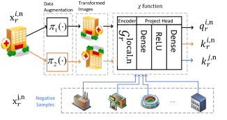
Figure 3: Encoding process

Next, the maximum number of iterations $\mathcal{N}_{k,t}^{n}$ of local training for vehicle $n$ is calculated according to Eq. (15) and Eq. (16) based on the downloaded CPU frequency $f_{k,t}^{n}$. Then each training vehicle retrains the local model for $\mathcal{N}_{k,t}^{n}$ iterations. Specifically, for each iteration $\psi_{k,t}^{n}\in[1,\mathcal{N}_{k,t}^{n}]$ of local training, each vehicle $n$ encodes the images of the local data, where the encoding process is illustrated in Fig. 3. For each image $x_{r}^{i,n}\in\left\{x_{r}^{1,n},\ x_{r}^{2,n},\ \ldots x_{r}^{i,n},\ldots x_{r}^{\mathcal{Z},n}\right\}$ in vehicle $n$ undergoes two different data augmentation methods $\pi_{1}(\cdot)$ and $\pi_{2}(\cdot)$, e.g., flipping, rotating, scaling, etc. We treat the remaining images, donated as $x_{r}^{j,n},j\in\left[1,\mathcal{Z}\right]\ \text{and}\ j\neq i$, as negative samples. Then, these two augmented images $\pi_{1}(x_{r}^{i,n})$ and $\pi_{2}(x_{r}^{i,n})$ along with $x_{r}^{j,n}$ are input into an $\chi$ function, which composed of an encoder with function $\mathcal{G}_{r}^{\text{local},n}$, and a project head including two dense neutral networks and a ReLU function. The $\chi$ function outputs anchor sample $q_{r}^{i,{n}}$, positive sample $k_{{r}}^{i,{n}}$, and encoded negative samples $k_{{r}}^{j,{n}}$, respectively, i.e.,

$$q_{r}^{i,n}=\chi\left\{\left[\pi_{1}\left(x_{r}^{i,n}\right)\right]\right\},\ i\in\left[1,\mathcal{Z}\right],$$ (37)

$$k_{r}^{i,n}=\chi\left\{\left[\pi_{2}\left(x_{r}^{i,n}\right)\right]\right\},\ i\in\left[1,\mathcal{Z}\right],$$ (38)

$$k_{r}^{j,n}=\chi\left\{\left(x_{r}^{j,n}\right)\right\},\ j\in\left[1,\mathcal{Z}\right],\ \text{and}\ j\neq i.$$ (39)

The dual temperature loss of the $i$-th image of anchor sample of the vehicle $n$ in round $r$ can be transformed into [22]

$$\begin{split}\mathcal{L}_{q_{{r}}^{i,n}}^{\text{DT}}\left(\theta_{{r}}^{\text{\text{local}},n},\ q_{{r}}^{i,n},\ k_{{r}}^{i,n},\ k_{{r}}^{j,n}\right)=-\text{sg}\left[\frac{{{(W}_{\beta})}_{{r}}^{i,n}}{{{(W}_{\alpha})}_{{r}}^{i,n}}\right]\\ \times\text{log}\frac{\exp{\left(\frac{q_{{r}}^{i,n}\cdot k_{{r}}^{i,n}}{\tau_{\alpha}}\right)}}{\exp{\left(\frac{q_{{r}}^{i,n}\cdot k_{{r}}^{i,n}}{\tau_{\alpha}}\right)}+\sum_{j=1}^{\mathcal{K}}\exp{\left(\frac{q_{{r}}^{i,n}\cdot k_{{r}}^{j,n}}{\tau_{\alpha}}\right)}},\end{split}$$ (40)

where $\text{sg}[\cdot]$ indicates the stop gradient, and

$$\begin{split}{{(W}_{\beta})}&{}_{{r}}^{i,n}=1-\\ &\frac{\exp{\left(\frac{q_{{r}}^{i,n}\cdot_{{r}}^{i,n}}{\tau_{\beta}}\right)}}{\exp{\left(\frac{q_{{r}}^{i,n}\cdot k_{{r}}^{i,n}}{\tau_{\beta}}\right)}+\sum_{j=1}^{\mathcal{K}}\exp{\left(\frac{q_{{r}}^{i,n}\cdot k_{{r}}^{j,n}}{\tau_{\beta}}\right)}},\end{split}$$ (41)

$$\begin{split}{{(W}_{\alpha})}&{}_{{r}}^{i,n}=1-\\ &\frac{\exp{\left(\frac{q_{{r}}^{i,n}\cdot k_{{r}}^{i,n}}{\tau_{\alpha}}\right)}}{\exp{\left(\frac{q_{{r}}^{i,n}\cdot k_{{r}}^{i,n}}{\tau_{\alpha}}\right)}+\sum_{j=1}^{\mathcal{K}}\exp{\left(\frac{q_{{r}}^{i,n}\cdot k_{{r}}^{j,n}}{\tau_{\alpha}}\right)}},\end{split}$$ (42)

where $\tau_{\alpha}$ and $\tau_{\beta}$ are temperature hyper-parameters [63], which that control the shape of the samples distribution, and $\mathcal{K}$ is the number of negative samples.

Then, for each image, the aim is to minimize the loss function and get optimize local mode $\hat{\theta}_{{r}}^{{\text{local}},n}$, i.e.,

$$\hat{\theta}_{{r}}^{{\text{local}},n} =\underset{\theta_{{r}}^{\text{local},n}}{\operatorname{argmin}}\frac{1}{\mathcal{Z}}\sum_{i=1}^{\mathcal{Z}}\mathcal{L}_{q_{{r}}^{i,n}}^{\text{DT}}\big{(}\theta_{{r}}^{{\text{local}},n},q_{{r}}^{i,n},$$ (43)

$$\hskip 113.81102ptk_{{r}}^{i,n},k_{{r}}^{j,n}\big{)},$$

where $\theta_{{r}}^{{\text{local},n}}$ represents the parameters of local model of vehicle $n$ in round $r$. Each vehicle approaches ${\hat{\theta}}_{{r}}^{{\text{local},n}}$ according to SGD method, and the process of updating is as follows:

$$\begin{split}\theta_{{r}}^{\text{local},n}\leftarrow\ &\theta_{{r}}^{\text{local},n}\\ &-\eta^{r}\nabla\mathcal{L}_{q_{{r}}^{i,n}}^{\text{DT}}\left(\theta_{{r}}^{\text{local},n},\ q_{{r}}^{i,n},\ k_{{r}}^{i,n},\ k_{{r}}^{j,n}\right),\end{split}$$ (44)

where $\eta^{r}$ represents the learning rate for round $r$, and $\nabla$ is the SGD algorithm. Repeat the local training $\mathcal{N}_{k,t}^{n}$ iterations and output the final local model $\theta_{{r}}^{\text{local},n}$.

Noting that during the local training process, the vehicle simultaneously captures $\mathcal{Z}$ new images $x_{r+1}^{i,n}$, $i\in\left[1,\mathcal{Z}\right]$ with the camera for the next round of local training. When the iterations reach to $\mathcal{N}_{k,t}^{n}$, the local training is finished, and outputs the final local model $\theta_{{r}}^{\text{local},n}$.

Step 3, Upload model: $N$ training vehicles employ downloaded transmission power to upload the trained local models $\left\{\theta_{{r}}^{{\text{local},1}},\theta_{{r}}^{{\text{local},2}},\ldots\theta_{{r}}^{{\text{local},n}}\ldots\theta_{{r}}^{{\text{local},N}}\right\}$ and the velocities $\left\{v_{k,t+1}^{1},v_{k,t+1}^{2},\ldots v_{k,t+1}^{n}\ldots v_{k,t+1}^{N}\right\}$ for slot $t+1$ based on the mobility model. Specifically, each vehicle will upload the local model $\theta_{{r}}^{{\text{local},n}}$ and $v_{k,t}^{n}$ with transmission power $p_{k,t}^{n}$ when local training is finished.

Step 4, Aggregation and Update: Firstly, $C_{k,t}^{n}(p_{k,t}^{n})$ can be calculated by Eq. (11) and Eq. (12) based on the transmission power $p_{k,t}^{n}$.

After receiving the trained models and velocities from $n$ training vehicles, the BS firstly calculates the blur level $\mathcal{B}_{r}^{n}$ based on the received velocity of vehicle $n$ in the previous slot, as [64][65]:

$$\mathcal{B}_{r}^{n}=\frac{sH}{Q}v_{k,t-1}^{n},$$ (45)

where $s$ is the focal length, $H$ is the exposure time interval, and $Q$ is pixel units.

According to Eq. (45), we assign smaller weights to the parameters obtained from training vehicles with higher blur levels in the local model, thus reducing the impact of the motion blur and improving the performance of the global model. Then the BS employs a weighted federated algorithm to aggregate the parameters of $N$ models based on the blur level $\mathcal{B}_{r}^{n}$. The expression for the aggregated new global model is

$$\theta_{r}^{\text{global}}=\sum_{n=1}^{N}\left[\frac{\left(\sum_{n=1}^{N}\mathcal{B}_{r}^{n}-\mathcal{B}_{r}^{n}\right)C_{k,t}^{n}(p_{k,t}^{n})\theta_{r}^{\text{local},n}}{\sum_{n=1}^{N}\left(\sum_{n=1}^{N}\mathcal{B}_{r}^{n}-\mathcal{B}_{r}^{n}\right)}\right],$$ (46)

where $\theta_{r}^{\text{global}}$ is the parameters of new global model.

At the same time, BS calculates the reward $r_{k,t}$ according to Eq. (36). After getting $r_{k,t}$, state $s_{k,t}$ transitions to $s_{k,t+1}$. BS saves the tuple $(s_{k,t},a_{k,t},r_{k,t},s_{k,t+1})$ to the replay buffer. When storing tuples, if the number of stored tuples is less than the storage capacity, the tuple is directly stored.

Repeat Step 2 to Step 4 until slot $t$ reaches to $S^{\text{max}}$. At this point, if the episode $k$ is divided by $K_{u}$, the five networks of SAC need to be updated, otherwise, it is not required. After that, episode $k$ moves to episode $k+1$, Slot $t$ reset to $0$. Next, we will introduce the update process.

In training stage, SAC algorithm optimizes the policy of actor network $\varsigma$ to achieve higher cumulative rewards while also maximizing the policy entropy. Our objective is to find the optimal policy $\pi^{\ast}(a_{k,t}|s_{k,t})$ of $\pi(a_{k,t}|s_{k,t})$ that maximizes both the long-term discounted rewards and the entropy of the policy simultaneously, i.e., maximum $\mathcal{J}(\pi(a_{k,t}|s_{k,t}))$, which can be expresses as

$$\mathcal{J}(\pi(a_{k,t}|s_{k,t}))=E_{s_{k,t}\sim\mathcal{D}}\sum_{t=1}^{\mathcal{S}^{\text{max}}}\left[\gamma^{t-1}r_{k,t}\right.\left.+\alpha H[\pi\left(\cdot\middle|s_{k,t}\right)]\right],$$ (47)

where $\mathcal{D}$ is the distribution of previously sampled states and actions. $\gamma\in[0,1]$ denotes the discount factor. $\pi\left(\cdot\middle|s_{k,t}\right)$ represents the policy after taking all actions in state $s_{k,t}$. $H[\pi\left(\cdot\middle|s_{k,t}\right)]=E[\text{log}\pi\left(\cdot\middle|s_{k,t}\right)]$, and signifies the policy entropy. $\alpha$ measures the weight on policy entropy while maximizing discounted rewards. Moreover, in state $s_{k,t}$, $\alpha$ can dynamically adjust based on the optimal $\alpha^{\ast}$, i.e.,

$$\alpha^{\ast}=-\arg\min_{\alpha}E[\alpha\log\pi^{\ast}(a_{k,t}|s_{k,t})+\alpha\widetilde{H}],$$ (48)

where $\widetilde{H}$ represents the dimensions of action $a_{k,t}$.

For each iteration of the updating process, randomly sample $\mathcal{M}$ tuples from the replay buffer to form a mini-batch for training. For the $m$-th tuple $(s_{m},a_{m},r_{m},s_{m+1})$ in the mini-batch, where $m\in[1,\mathcal{M}]$, inputting $s_{m}$ to the actor network to obtain $a_{m}^{\prime}$. It is worth noting that this action $a_{m}^{\prime}$ is not the same as $a_{m}$ in the tuple. Thus, the gradient of loss function of $\alpha$ can be calculated as

$$\nabla_{\alpha}\mathcal{J}_{\alpha}=\nabla_{\alpha}E\Big{[}-\frac{1}{\mathcal{M}}\sum_{m=1}^{\mathcal{M}}\left[\alpha\log\pi_{\varsigma}(a_{m}^{\prime}|s_{m})+\alpha\widetilde{H}\right]^{2}\Big{]}.$$ (49)

Feeding $(s_{m},a_{m}^{\prime})$ into the two critic networks $\xi_{1}$ and $\xi_{2}$, and then produce the corresponding action value functions $Q_{\xi_{1}}\left(s_{m},a_{m}^{\prime}\right)$ and $Q_{\xi_{2}}\left(s_{m},a_{m}^{\prime}\right)$. ${Q}_{\xi}\left(s_{m},a_{m}^{\prime}\right)$ is donated as the smaller between $Q_{\xi_{1}}\left(s_{m},a_{m}^{\prime}\right)$ and $Q_{\xi_{2}}\left(s_{m},a_{m}^{\prime}\right)$, and can be expressed as

$${Q}_{\xi}\left(s_{m},a_{m}^{\prime}\right)=\min\left[Q_{\xi_{1}}\left(s_{m},a_{m}^{\prime}\right),Q_{\xi_{2}}\left(s_{m},a_{m}^{\prime}\right)\right].$$ (50)

Therefore, the the gradient of loss of the actor network parameters can be calculated by

$$\begin{split}&\nabla_{\varsigma}\mathcal{J}_{\varsigma}=\nabla_{\varsigma}\left[-\frac{1}{\mathcal{M}}\sum_{m=1}^{\mathcal{M}}\left[\alpha\text{log}\pi_{\varsigma}\left(a_{m}^{\prime}\middle|s_{m}\right)\right]^{2}\right]+\\ &\nabla_{\varsigma}\left[-\frac{1}{\mathcal{M}}\sum_{m=1}^{\mathcal{M}}\left[{Q}_{\xi}(s_{m},a_{m}^{\prime})-\alpha\text{log}\pi_{\varsigma}\left(a_{m}^{\prime}\middle|s_{m}\right)\right]^{2}\right]\\ &\times\nabla_{\varsigma}f_{\varsigma}(o;s_{m}),\end{split}$$ (51)

where $o$ is noise drawn from a multivariate normal distribution, such as a spherical Gaussian, and $f_{\varsigma}(o;s_{m})$ is a function used to reparameterize action $a_{m}^{\prime}$ [67]. Finally, the actor network is updated by SGD method.

Input: $\gamma$, $\alpha$, $\varsigma$, $\xi_{1}$, $\xi_{2}$, $\varpi_{1}$, $\varpi_{2}$, $\mathcal{M}$, $k$, $K_{t}$

Function UPDATE($\gamma$, $\alpha$, $\varsigma$, $\xi_{1}$, $\xi_{2}$, $\varpi_{1}$, $\varpi_{2}$, $\mathcal{M}$, $k$, $K_{t}$):

      

      Randomly sample $\mathcal{M}$ tuples from replay buffer

      Update $\alpha$ according to Eq. (49);

      Update $\varsigma$ according to Eq. (51);

      Update $\xi_{1}$ and $\xi_{2}$ according to Eq. (52) and Eq. (53);

      if $k\mod K_{t}=0$ then

             Update $\varpi_{1}$ and $\varpi_{2}$ according to Eq. (55) and Eq. (56);

      

Algorithm 1 The process of updating networks of SAC Algorithm

Input: $\theta^{0}$, $\varsigma$, $\xi_{1}$, $\xi_{2}$, $\varpi_{1}$, $\varpi_{2}$

Initialize round $r\leftarrow 0$, episode $k\leftarrow 0$;

for episode $k$ from $1$ to $K^{\text{max}}$ do

       slot $t\leftarrow 0$;

       for slot $t$ from $1$ to $S^{\text{max}}$ do

             $r\leftarrow(k-1)\cdot S^{\text{max}}+t$;

             Obtain state $s_{k,t}$ based on distance and velocity;

             Get action $a_{k,t}$ through SAC algorithm;

             for $n=1,2,\dots,N$ in parallel do

                   Download global model $\theta_{r-1}^{\text{global}}$, $p_{k,t}^{n}$, and $f_{k,t}^{n}$;

                   $\theta_{r}^{{\text{local}},n}\leftarrow\text{LOCAL}(\theta_{r-1}^{\text{global}},p_{k,t}^{n},f_{k,t}^{n})$;

                  

            if $r=1$ then

                   Vehicle $n\in[1,N]$ uploads the local model $\theta_{r}^{{\text{local}},n}$ and $v_{k,t}^{n}$ to BS with download transmission power $p_{k,t}^{n}$, along with velocity $v_{0}^{n}$;

                  

            else

                   Vehicle $n\in[1,N]$ uploads the local model $\theta_{r}^{{\text{local}},n}$ and $v_{k,t}^{n}$ to BS with download transmission power $p_{k,t}^{n}$;

                  

            BS aggregates received local models based on $\mathcal{B}_{r}^{n}$ and updates $\theta_{r}^{\text{global}}$ according to Eq. (46);

             Save $\theta_{r}^{\text{global}}$ to global model;

            

      if episode $k$ mod $K_{u}$ = 0 then

             UPDATE($\gamma$, $\alpha$, $\varsigma$, $\xi_{1}$, $\xi_{2}$, $\varpi_{1}$, $\varpi_{2}$);

            

      

Function Local($\theta_{r-1}^{\text{global}},p_{k,t}^{n},f_{k,t}^{n}$):

       Input: $\theta_{r-1}^{\text{global}},p_{k,t}^{n},f_{k,t}^{n}$

       Set the parameter of global model $\theta_{r-1}^{\text{global}}$ to local model $\theta_{r}^{{\text{local}},n}$;

       Calculate iteration value $\mathcal{N}_{k,t}^{n}$ according to Eq. (15) and Eq. (16);

       for each iteration $\psi_{k,t}^{n}$ from $1$ to $\mathcal{N}_{k,t}^{n}$ do

             Prepare local model $\theta_{r}^{{\text{local}},n}$;

             for image $i$ from $1$ to $\mathcal{Z}$ do

                   Calculate $q_{r}^{i,n}$, $k_{r}^{i,n}$, and $k_{r}^{j,n}$ according to Eq. (37) - Eq. (39);

                  

            Calculate the average loss of $\mathcal{Z}$ images according to Eq. (40) - Eq. (42), and update $\theta_{r}^{{\text{local}},n}$ according to SGD algorithm in Eq. (44);

            

      Output: $\theta_{r}^{{\text{local}},n}$

      

Algorithm 2 The DRL-BFSSL Algorithm

For updating critic networks $\xi_{1}$ and $\xi_{2}$, firstly, we use $(s_{m},a_{m})$ as input and feed it separately into the critic networks $\xi_{1}$ and $\xi_{2}$, and obtain the action values pairs $Q_{\xi_{1}}\left(s_{m},a_{m}\right)$ and $Q_{\xi_{2}}\left(s_{m},a_{m}\right)$, respectively. Additionally, input $s_{m+1}$ into the actor network to obtain $a_{m+1}$, and represented as $\text{log}\pi_{\varsigma}^{m+1}(a_{m+1}|s_{m+1})$ which is to convert the policy parameter space into real number space, and this transformation helps with the computational efficiency and numerical stability of the optimization algorithm. Finally, use $\left(s_{m+1},a_{m+1}\right)$ as input for the two target networks $\varpi_{1}$ and $\varpi_{2}$, and output the action value pairs $Q_{\varpi_{1}}\left(s_{m+1},a_{m+1}\right)$ and $Q_{\varpi_{2}}\left(s_{m+1},a_{m+1}\right)$. We take the minimum of the two, denoted as $Q_{\varpi}\left(s_{m+1},a_{m+1}\right)$. From this, we can calculate the target value $\hat{Q}(s_{m+1},a_{m+1})$ as

$$\begin{split}\hat{Q}(s_{m+1},a_{m+1})=&Q_{\varpi}(s_{m+1},a_{m+1})\\ &-\alpha\log\pi_{\varsigma}^{m+1}\left(a_{m+1}\middle|s_{m+1}\right),\end{split}$$ (52)

and the gradient of loss of critic networks $\xi_{1}$ and $\xi_{2}$ can be calculated as, respectively

$$\begin{split}\nabla_{\xi_{1}}\mathcal{J}_{\xi_{1}}=\nabla_{\xi_{1}}\Big{[}-\frac{1}{\mathcal{M}}\sum_{m=1}^{\mathcal{M}}{[r_{m}+\gamma\hat{Q}(s_{m+1},a_{m+1})}\\ \quad-Q_{\xi_{1}}(s_{m},a_{m})]^{2}\Big{]},\end{split}$$ (53)

$$\begin{split}\nabla_{\xi_{2}}\mathcal{J}_{\xi_{2}}=\nabla_{\xi_{2}}\Big{[}-\frac{1}{\mathcal{M}}\sum_{m=1}^{\mathcal{M}}{[r_{m}+\gamma\hat{Q}(s_{m+1},a_{m+1})}\\ \quad-Q_{\xi_{2}}(s_{m},a_{m})]^{2}\Big{]}.\end{split}$$ (54)

Finally, SGD method is employed to update the two critic networks. We also need to update both target networks for every $K_{t}$ iterations during this process. The updates for the two target networks are as follows

$$\varpi_{1}=\delta_{1}\ \xi_{1}+(1-\delta_{1})\varpi_{1},$$ (55)

$$\varpi_{2}=\delta_{2}\ \xi_{2}+(1-\delta_{2})\varpi_{2},$$ (56)

where $\delta_{1}$ and $\delta_{2}$ are constants much smaller than $1$. The pseudocode of the process of updating SAC networks is shown in Algorithm 1.

When episode $k$ reaches to $K^{\text{max}}$ and slot $t$ reached to $S^{\text{max}}$, we get a global model and an optimal parameter of actor network $\varsigma$, denoted as $\varsigma^{\ast}$. The pseudocode of complete algorithm is shown in Algorithm 2.

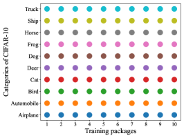
((a)) CIFAR-10 IID

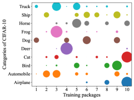
((b)) CIFAR-10 Non-IID, $\mu=0.1$

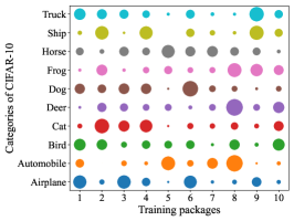
((c)) CIFAR-10 Non-IID, $\mu=1$

Figure 4: Data category distribution plot

VI Simulation Results

Python 3.10 is utilized to conduct the simulations, which are based on the scenarios outlined in the Section III. The simulation parameters are detailed in Table I.

TABLE I: Hyper-parameter

Parameter	Value	Parameter	Value
$m$	0.023	$\epsilon_{\tau}$	0.2
$\tau_{\alpha}$	0.1	$\tau_{\beta}$	1
$\mathcal{K}$	512	$\gamma$	0.99
$\delta_{1}/\delta_{2}$	0.001	Initial learning rate	0.06
$K^{\text{max}}$	1000	$S^{\text{max}}$	100
$Z$	11.2M	$B^{U}$	$2\times{10}^{6}Hz$
$N_{0}$	-114dB	$\xi$	8
$\kappa$	${10}^{-27}$	momentum of SGD	0.9
$f^{\text{min}}$	$5\times{10}^{7}Hz$	$f^{\text{max}}$	$4\times{10}^{8}Hz$
$p^{\text{min}}$	5dB	$p^{\text{max}}$	200dB
$T$	0.5s	$t_{\text{max}}^{\text{Trans}}$	0.02s
$\lambda_{1}$	0.7	$\lambda_{2}$	0.3
$v^{\text{min}}$	60km/h	$v^{\text{max}}$	150km/h
$\mu$	0.5	$\sigma^{2}$	8
$\vartheta_{1}$	0.05	$\vartheta_{2}$	$5\times{10}^{-5}$
$\mathcal{M}$	256	$\varepsilon_{1}/\varepsilon_{2}/\varepsilon_{3}$	0.3/0.3/0.4
$K_{u}$	2	$K_{t}$	80

We employ a modified ResNet-18, with a fixed dimension of 128-D, as the backbone model and utilize SGD with momentum as the optimizer. Momentum SGD is characterized by its strong randomness, rapid convergence, and ease of implementation, making it well-suited for optimizing the backbone model. Additionally, inspired by the concept of Cosine Annealing, we gradually reduce the learning rate at different stages of training to enhance the model’s training effectiveness.

Datasets: We utilize CIFAR-10 as the datasets, in which training datasets comprises 50,000 images distributed across 10 distinct categories, each of which consists 5,000 images. The testing datasets comprises 10000 images. We also establish two types of data distribution, including Independent and IID and Non-IID.

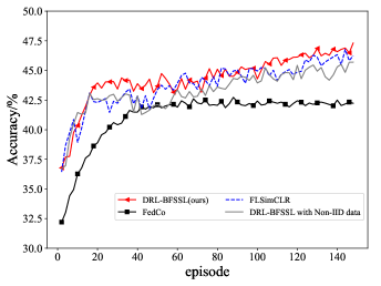
Figure 5: Comparison of DRL-BFSSL with Other Methods

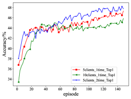
((a)) The accuracy of Top1

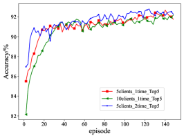
((b)) The accuracy of Top5

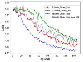
((c)) Loss function

Figure 6: Comparison of accuracy and loss

(1) IID: Data obeying an IID are mutually independent and share the same distribution. Simultaneously, the statistical properties among data are similar, facilitating the generalization of the model. We uniformly allocate the 50,000 image data from CIFAR-10 to 95 training packages, ensuring that each training package has at least 520 images available. In Fig. 4, we show the distribution of image data categories on 10 training packages. As shown in Fig. 4(a), the quantity of each image data category on each vehicle is equal, indicating a uniform distribution state.

(2) Non-IID: IID offers theoretical convenience, but in practical scenarios, data satisfied with IID is rare. Therefore, it is beneficial to evaluate the model’s training performance under Non-IID conditions for transferring the model to real-world scenarios [66]. As depicted in Fig. 4(b) and 4(c), scenarios with Dirichlet distribution parameters $\alpha$ set to 0.1 and 1 are respectively shown. It can be observed that as $\alpha$ decreases, the gap between different categories increases, while a larger $\alpha$ makes the distribution closer to IID. We set the Dirichlet distribution parameter $\alpha$ to 0.1 to simulate Non-IID data in IoV, aiming to simulate situations where each training vehicle, due to limited perspectives and environmental constraints, collects images with uneven category distributions. Therefore, for CIFAR-10, we ensure that each training package has at least 515 Non-IID images.

Testing: We rank the predicted labels based on their probabilities from highest to lowest. If the most probable predicted label (i.e., the top label) matches the true label, the prediction is considered correct, and this is referred to as the Top1 accuracy. If the true label is among the top five predicted labels, the prediction is also considered correct, and this is referred to as the Top5 accuracy. For testing the performance of SAC algorithm, we employ the output $\varsigma^{\ast}$ to obtain $\pi^{\ast}(a_{k,t}|s_{k,t})$. Each experiment is conducted for three times, and the final result is the average of these three experiments.

We first test the classification accuracy of the global model obtained under different conditions. We assume that each episode consists of 95 training packages, with each vehicle selecting one training package for each training session. When all training packages are used up, one episode is finished.

In Fig. 5, we compare our algorithm (DRL-BFSSL) with FedCo[34] and FLSimCLR[27], under the same number of iterations for local training. We also conducted experiments on Non-IID datasets. It can be observed that the classification accuracy of all three methods shows an upward trend after training. Among these methods, the FedCo algorithm starts with the lowest accuracy and continues to perform the worst during subsequent training. In contrast, DRL-BFSSL and FLSimCLR exhibit similar accuracy trends, but overall, DRL-BFSSL outperforms FLSimCLR in Top1 accuracy. The training performance on Non-IID datasets was slightly inferior to that on IID datasets but still superior to the FedCo and FLSimCLR algorithms.

The lower performance of FedCo can be attributed to the process described in FedCo[34], where in round $r$, each training vehicle uploads all stored $k$ values (with a batch size set to 512 in the experiment) to BS with a global queue set to 4096 to update the global direction. Updating the queue with $k$ values from different training vehicles compromises the Negative-Negative consistency requirement in MoCo, resulting in lower accuracy for these methods. Conversely, we also implemented the FLSimCLR, which requires a large number of negative samples. FLSimCLR performs worse than DRL-BFSSL primarily due to its dependency on a large number of negative samples to learn effective representations, whereas in our experiments, we used only a few negative samples. While this approach works well in centralized settings, it faces challenges in federated environments where the distribution of negative samples may not be consistent across different clients. The slightly lower performance on Non-IID data can be attributed to the inherent challenges in ensuring uniform representation across heterogeneous data distributions, which affects the overall consistency and learning efficiency in federated settings.

In Fig. 6, we examine scenarios where 5 and 10 training vehicles participate in each round of DRL-BFSSL and scenarios with different local iterations. The red and green lines in Fig. 6(a) represent scenarios with 5 and 10 training vehicles, respectively. It shows an improvement in model accuracy as few vehicles participate. This indicates that as the number of vehicles participating in each round of DRL-BFSSL increases, the number of iterations decreases, indicating fewer communication rounds between training vehicles and the BS. More interactions between vehicles and the BS lead to better model performance. The red and blue lines represent scenarios with 5 training vehicles participating in DRL-BFSSL per round. The red line indicates that training vehicles perform one local iteration, while the blue line indicates two local iterations. It can be observed that the results of two internal iterations surpass those of one iteration, highlighting the advantage of multiple local training iterations even when using the same set of images for local training. We can also observe that when 10 vehicles participate in each round of DRL-BFSSL, the initial accuracy is the lowest, and as the training rounds increase, it gradually becomes comparable to the accuracy achieved with 5 vehicles. This is because initially, the participating vehicles contribute diverse datasets. However, as the number of iterations increases, the newly added vehicles’ datasets become more similar, resulting in reduced datasets diversity. In this scenario, aggregating a small number of models in the initial stages yields better results because these models represent a wider range of datasets diversity.

In Fig. 6(b), the Top5 accuracy under the same training conditions as Fig. 6(a) is displayed. The trend of the curves is similar to that in Fig. 6(a), but the gaps between the curves are narrowing, and the accuracy is significantly improved. This suggests that the model becomes more robust and comprehensive when considering more candidate classes. This can be interpreted as the model demonstrating greater tolerance in multi-class classification, being more likely to include the correct classes and better handling the classification uncertainty of certain samples.

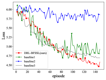
Figure 7: The loss of models aggregated with different weights

As shown in Fig. 6(c), we compare the loss curves of the trained models in Fig. 6(a) with the loss function of 5 vehicles after one round of training on the non-IID datasets. It can be observed that the loss function of each experiment exhibits a decreasing trend. Moreover, when 5 vehicles participate in each round of training with each vehicle conducting 2 iterations of local training, the loss decreases the fastest and reaches the minimum value. At the same time, compared to the curves on the IID training set, the loss function of the model trained on the Non-IID datasets exhibits significant fluctuations in the initial stage. However, as the number of episodes increases, the trend of the loss function gradually becomes similar to that on the IID datasets. This phenomenon can be partially attributed to the characteristics of the non-IID datasets. Due to the uneven distribution and diversity of data on the Non-IID datasets, the model faces greater challenges during training. Therefore, the loss function of the model may exhibit significant fluctuations in the initial stage. As training progresses, the model gradually adapts to the data distribution, leading to a reduction in the fluctuation of the loss function, ultimately stabilizing. Additionally, multiple rounds of internal training help the model better learn data features, allowing it to achieve lower loss values in a shorter time.

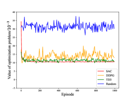
((a)) Optimization problem Comparison

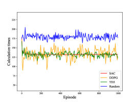
((b)) Calculation Comparison

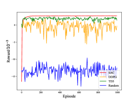
((c)) Reward Comparison

Figure 8: Comparison between different algorithms

All the above experiments assume that the images collected on the training vehicles are not affected by blurriness. Following, we will simulate the situation where some images appear motion blurred due to vehicle motion. We assume that if the velocity of training vehicles exceeds $100\text{km/h}$, 1/5 of the collected image data will experience motion blur. Vehicles continue to use these images to train local models, which are then uploaded.

In Fig. 7, we adopt three aggregation methods, including DRL-BFSSL and two baseline algorithms, to aggregate for obtaining a global model with $1/5$ blurred images. Meanwhile, we introduce $3/5$ of blurred images to obtain a global model using the DRL-BFSSL method. From the figure, it can be observed that the loss curves of all four methods exhibit a decreasing trend. Specifically, baseline1 represents the BS uniformly utilizing the average federated aggregation model parameters. Baseline2 represents the BS discarding models trained by blurry image data, and then using average federated to aggregate model parameters. To validate the impact of blurry images on the model, we have set up baseline3, where $3/5$ of the images experience motion blur.

Based on the results of baseline1 and baseline2, it is evident that although baseline1 does not achieve a stable convergence of loss function, compared to baseline2, its loss function reaches a smaller value. In other words, because baseline2 discards some models during aggregation, baseline2 uses the fewest number of models among these methods. This suggests that the number of models participating in aggregation is more critical than the quality of the models. Finally, our proposed aggregation method of DRL-BFSSL not only reduces the fluctuation of the loss function but also converge to a smaller value. Comparing with baseline3, it can be observed that an increasing number of blurry image data is unfavorable for the convergence of the loss function. However, compared to other aggregation methods, the convergence speed remains relatively stable.

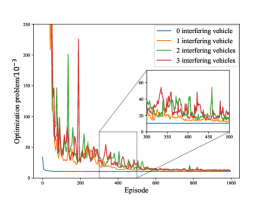
((a)) Optimization problem Comparison

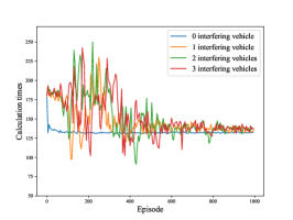
((b)) Calculation Comparison

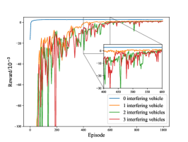
((c)) Reward Comparison

Figure 9: Comparison between different number of interference vehicles

In Fig. 8, we compare the performance of SAC, DDPG, TD3, and Random algorithms in solving the optimization problem, covering the optimal results, computation times, and reward functions. From Fig. 8(a), it is evident that the SAC algorithm rapidly reaches convergence and remains stable, while DDPG and TD3 show similar performance, with TD3 slightly outperforming DDPG. Although DDPG and TD3 exhibit some convergence trends, they are highly volatile and less stable. In contrast, the optimal solution obtained by the Random algorithm is significantly higher than that achieved by the SAC algorithm. Overall, the SAC algorithm can obtain better solutions more quickly and stably. This is mainly because SAC introduces entropy rewards to encourage policy exploration, maintaining a certain level of exploration during training.

In Fig. 8(b), we presents a comparison of calculation times. The SAC algorithm reaches a stable value in terms of computation times, while the calculation times of the DDPG algorithm fluctuate significantly. TD3 algorithm shows a similar trend to DDPG algorithm, but with smaller fluctuations. The calculation times for both DDPG algorithm and TD3 algorithm fluctuate around the stable value achieved by SAC. The Random algorithm consistently has higher calculation times than the SAC algorithm, indicating that it has not balanced the optimal problem with calculation times. We aim to have sufficient calculation times to facilitate the training of the global model while minimizing the value of optimization problem. The SAC algorithm excels in this aspect as it can utilize each update more efficiently, enhancing training efficiency. Fig. 8(c) shows the reward functions for each algorithm. The overall reward value of the SAC algorithm is higher than that of DDPG, TD3, and the Random algorithm. The DDPG algorithm might be affected by gradient instability when updating policies, leading to significant fluctuations during its convergence process. In contrast, TD3 algorithm exhibits less fluctuation but still has lower reward values than SAC algorithm. The Random algorithm, due to its inherent randomness, cannot effectively explore the solution space.

In Fig. 9, we compare the performance of the SAC algorithm under different numbers of interfering vehicles, including the value of optimization problem, calculation times and the reward function. Overall, the results of the three can converge to relatively stable values. Specifically, Fig. 9(a) illustrates the optimal solutions under the SAC algorithm in the presence of varying numbers of interfering vehicles. When there are no interfering vehicles, the optimal solution converges to a minimum value and remains stable. However, with the introduction of interfering vehicles, the optimal solution noticeably increases. Despite this increase, as the number of interfering vehicles continues to grow, the optimal solution does not vary significantly, but ultimately converging to a relatively small and stable value. This behavior can be attributed to the SAC algorithm’s ability to adapt to increased complexity and interference, effectively maintaining a robust performance even under more challenging conditions. Fig. 9(b) shows that when there are no interfering vehicles, the calculation times converge to its minimum value the fastest. As the number of interfering vehicles increases, the convergence value also rises. This is because when the number of interfering vehicles increases, the system needs to allocate more energy to the vehicles for training. Fig. 9(c) shows a comparison of the reward function throughout the process. In general, when there are no interfering vehicles, the reward function can quickly converge to a higher value. However, as the number of interfering vehicles increases, the reward function decreases. At the same time, it can be seen that as long as interfering vehicles are introduced, the overall system reward will significantly decrease. This indicates that once interfering vehicles are added, the overall system reward will drop significantly. The increase in interfering vehicles makes management and energy allocation more complex, thereby reducing the efficiency and effectiveness of the SAC algorithm.

With the absence of interfering vehicles, we train models using both the SAC, DDPG, TD3 and Random algorithms and saved their parameters for testing. As shown in Fig. 10, the overall results indicate that the optimization problem solutions produced by the SAC algorithm are smaller and more stable compared to those produced by the other algorithms. This suggests that the SAC algorithm outperforms the other algorithms in terms of both stability and performance. This superiority is likely due to the entropy regularization strategy employed by the SAC algorithm, which allows for a better balance between exploration and exploitation, leading to more stable convergence to superior solutions. In contrast, the DDPG and TD3 algorithm may be more prone to getting stuck in local optima during policy optimization, resulting in lower quality and less stable solutions.

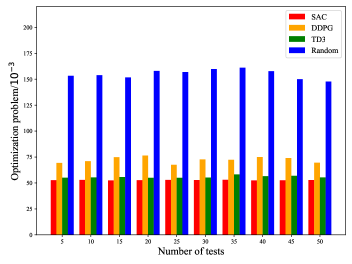
Figure 10: Testing results

VII Conclusions

In this paper, we proposed the DRL-BFSSL algorithm, which ensures privacy protection and avoid the data labeling. It also addressed aggregation challenges causing by motion blur in IoV. Additionally, we introduced a resource allocation strategy based on the SAC algorithm to minimize energy consumption and delay for computing and model transmission, during this process, employed packet error rate to set a minimum transmission power to ensure that the BS can successfully receive the local models uploaded by vehicles. The conclusions are summarized as follows:

• We proposed the DRL-BFSSL algorithm, which protects user privacy, eliminates the need for labels in local training and achieves higher classification accuracy on both IID and Non-IID datasets.

• For the case of blurred images in IoV, our proposed aggregation method can effectively resist motion blur, resulting in a steady decrease in the loss function.

• Based on the SAC algorithm, our proposed resource allocation scheme minimizes energy consumption and delay while maintaining a stable number of calculation times and achieving high rewards. Even with interference, this algorithm still obtains high and stable rewards.

Appendix A

According to Eq. (26), let $\varphi=\max{\left(\frac{E}{\beta_{k,t}^{n}}+\frac{F}{f_{k,t}^{n}}\right)}$, and Eq. (18) can be obtained:

$$\begin{split}\underset{\boldsymbol{\beta},\boldsymbol{p},\boldsymbol{f}}{\min}\mathcal{C}:&\sum_{n=1}^{N}\left[\frac{A}{\beta_{k,t}^{n}}+B\left({f_{k,t}^{n}}\right)^{3}-C\left({f_{k,t}^{n}}\right)^{2}\right]+\varphi.\end{split}$$ (57)

s.t.

$$0<\beta_{k,t}^{n}<1$$ (57a)

$$\sum_{n=1}^{N}\beta_{k,t}^{n}\leq 1$$ (57b)

$$\epsilon_{k,t}^{n}\leq\epsilon_{\tau}$$ (57c)

$$p^{\text{min}}\leq p_{k,t}^{n}\leq p^{\text{max}}$$ (57d)

$$f^{\text{min}}\leq f_{k,t}^{n}\leq f^{\text{max}}$$ (57e)

$$\frac{E}{\beta_{k,t}^{n}}+\frac{F}{f_{k,t}^{n}}\leq\varphi$$ (57f)

Theorem1: The subproblem of the optimization problem (26) is a convex function.

Proof: The formula $\mathcal{C}$ consists of four parts: $\frac{A}{\beta_{k,t}^{n}}$, $B\left({f_{k,t}^{n}}\right)^{3}$, $C\left({f_{k,t}^{n}}\right)^{2}$ and $\varphi$. Since each part is a convex function and the constraints are all affine, so Eq. (26) is also a convex function.

Using the Lagrange Multiplier Method to find the extreme values of a multivariable function subject to multiple constraints, the Lagrange equation can be expressed as:

$$\begin{split}\mathcal{C}=&\sum_{n=1}^{N}\left[\frac{A}{\beta_{k,t}^{n}}+B\left({f_{k,t}^{n}}\right)^{3}-C\left({f_{k,t}^{n}}\right)^{2}\right]\\ &+\varphi+\phi\left(\sum_{n=1}^{N}\beta_{k,t}^{n}-1\right)+\tau\left(\frac{E}{\beta_{k,t}^{n}}+\frac{F}{f_{k,t}^{n}}-\varphi\right),\end{split}$$ (59)

where $\phi$ and $\tau$ are Lagrange Multipliers associated with constraints (57b) and (57f), utilizing the KKT conditions, we have the following equations:

$$\frac{\partial\mathcal{C}}{\partial\beta_{k,t}^{n}}=\phi-\frac{A+\tau E}{{\left(\beta_{k,t}^{n}\right)}^{2}}=0,$$ (60)

$$\frac{\partial\mathcal{C}}{\partial f_{k,t}^{n}}=3B\left({f_{k,t}^{n}}\right)^{2}-2Cf_{k,t}^{n}-\frac{\tau F}{{\left({f_{k,t}^{n}}\right)^{2}}}=0,$$ (61)

$$\phi\left(\sum_{n=1}^{N}\beta_{k,t}^{n}-1\right)=0,$$ (62)

$$\tau\left(\frac{E}{\beta_{k,t}^{n}}+\frac{F}{f_{k,t}^{n}}-\varphi\right)=0.$$ (63)

From Eq. (60) and Eq. (61), we can derive out

$$\phi=\frac{A+\tau E}{\left({\beta_{k,t}^{n}}\right)^{2}},$$ (64)

$$\frac{3B\left({f_{k,t}^{n}}\right)^{4}-2C\left({f_{k,t}^{n}}\right)^{3}}{F}=\tau.$$ (65)

By transforming Eq. (64), we can obtain:

$$\beta_{k,t}^{n}=\frac{\left(A+\tau E\right)^{\frac{1}{2}}}{\phi^{\frac{1}{2}}},$$ (66)

and from Eq. (62), we can get

$$\phi\sum_{n=1}^{N}{\beta_{k,t}^{n}=\phi}.$$ (67)

Substitute Eq. (66) into Eq. (67), we can obtain

$$\sum_{n=1}^{N}\left(A+\tau E\right)^{\frac{1}{2}}=\phi^{\frac{1}{2}},$$ (68)

Substitute Eq. (68) into Eq. (66), the final result can be obtained:

$$\beta_{k,t}^{n}=\frac{{(A+\tau E)}^{\frac{1}{2}}}{\sum_{n=1}^{N}{(A+\tau E)}^{\frac{1}{2}}},$$ (69)

where

$$\tau=\frac{3B\left({f_{k,t}^{n}}\right)^{4}-2C\left({f_{k,t}^{n}}\right)^{3}}{F}.$$ (70)

References

- [1] Q. Wu, Y. Zhao, Q. Fan, P. Fan, J. Wang and C. Zhang, “Mobility-Aware Cooperative Caching in Vehicular Edge Computing Based on Asynchronous Federated and Deep Reinforcement Learning,” IEEE journal of selected topics in signal processing, vol. 17, no.1, pp. 66-81, 2023.
- [2] K. Zheng, Q. Zheng, P. Chatzimisios, W. Xiang, and Y. Zhou, “Heterogeneous vehicular networking: A survey on Architecture, Challenges, and Solutions,”IEEE Communication Surveys Tutorials, vol. 17, no. 4, pp. 2377-2396, doi:10.1109/COMST.2015.2440103, 4th Quart., 2015.
- [3] Q. Wu, Y. Zhao, Q. Fan, P. Fan, J. Wang, and C. Zhang, “Mobility-Aware Cooperative Caching in Vehicular Edge Computing Based on Asynchronous Federated and Deep Reinforcement Learning”, IEEE Journal of Selected Topics in Signal Processing, vol. 17, no. 1, pp. 66-81, Jan. 2023.
- [4] G. Luo, C. Shao, N. Cheng, H. Zhou, H. Zhang, Q. Yuan, and J. Li, “EdgeCooper: Network-Aware Cooperative LiDAR Perception for Enhanced Vehicular Awareness,”IEEE Journal on Selected Areas in Communications, vol. 42, issue. 1, pp. 207-222, doi:10.1109/JSAC.2023.3322764, Jan. 2024.
- [5] Q. Wu, S. Shi, Z. Wan, Q. Fan, P. Fan, and C. Zhang, “Towards V2I Age-aware Fairness Access: A DQN Based Intelligent Vehicular Node Training and Test Method”, Chinese Journal of Electronics, vol. 32, no. 6, pp. 1230-1244, 2023.
- [6] K. Wang, F. Yu, L. Wang, J. Li, N. Zhao, Q. Guan, B. Li, and Qiong Wu, “Interference Alignment with Adaptive Power Allocation in Full-Duplex-Enabled Small Cell Networks,” IEEE Transactions on Vehicular Technology, vol. 68, No. 3, Mar. 2019.
- [7] J. Shen, N. Cheng, X. Wang, F. Lyu, W. Xu, Z. Liu, K. Aldubaikhy, and X. Shen, “RingSFL: An Adaptive Split Federated Learning Towards Taming Client Heterogeneity,” IEEE Transactions on Mobile Computing, vol. 23, no. 5, pp. 5462-5478, DOI: 10.1109/TMC.2023.3309633, May. 2024.
- [8] Q. Wu, S. Wang, H. Ge, P. Fan, Q. Fan, and K. B. Letaief, “Delay-sensitive Task Offloading in Vehicular Fog Computing-Assisted Platoons”, IEEE Transactions on Network and Service Management, vol. 21, no. 2, pp. 2012-2026, Apr. 2024.
- [9] Q. Wu, H. Liu, C. Zhang, Q. Fan, Z. Li, and K. Wang, “Trajectory Protection Schemes Based on a Gravity Mobility Model in IoT,” Electronics, vol. 8, no. 148, Feb. 2019.
- [10] D. Ye, R. Yu, M. Pan, and Z. Han, “Federated learning in vehicular edge computing: A selective model aggregation approach,” IEEE Access, vol. 8, pp. 23920–23935, doi:10.1109/ACCESS.2020.2968399,2020.
- [11] C. Mi, Y. Huang, C. Fu, Z. Zhang, and O. Postolache, “Vision-Based Measurement: Actualities and Developing Trends in Automated Container Terminals,”IEEE Instrumentation and Measurement Magazine, vol. 24, issue. 4, pp. 65-76, doi: 10.1109/MIM.2021.9448257, Jun.2021.
- [12] V. Gupta, V. Mishra, P. Singhal, and A. Kumar, “An Overview of Supervised Machine Learning Algorithm,” 2022 11th International Conference on System Modeling and Advancement in Research Trends (SMART)”, doi:10.1109/SMART55829.2022.1004761824, Feb.2023.
- [13] Q. Wu, S. Xia, P. Fan, Q. Fan, and Z. Li, “Velocity-Adaptive V2I Fair Access Scheme Based on IEEE 802.11 DCF for Platooning Vehicles,” Sensors, vol. 18, no. 12, Art no. 4198, Dec. 2018
- [14] J. Fan, S. Yin, Q. Wu, and F. Gao, “Study on Refined Deployment of Wireless Mesh Sensor Network,” in Proc. of IEEE International Conference on Wireless Communications, Networking and Mobile Computing (WICOM’10), Chengdu, China, pp. 370-375, Jul. 2010.
- [15] K. He, H. Fan, Y. Wu, S. Xie, and R. Girshick,“Momentum contrast for unsupervised visual representation learning,”2020 IEEE/CVF Conference on Computer Vision and Pattern Recognition (CVPR), doi: 10.1109/CVPR42600.2020.00975, Aug. 2020.
- [16] Q. Wu, S. Nie, P. Fan, H. Liu, Q. Fan, and Z. Li, “A Swarming Approach to Optimize the One-Hop Delay in Smart Driving Inter-Platoon Communications,” Sensors, vol. 18, no. 10, Art. no. 3307, Oct. 2018.
- [17] J. Zhao, R. Li, H. Wang, and Z. Xu, “HotFed: Hot Start through Self-Supervised Learning in Federated Learning”2021 IEEE 23rd Int Conf on High Performance Computing and Communications; 7th Int Conf on Data Science and Systems; 19th Int Conf on Smart City; 7th Int Conf on Dependability in Sensor, Cloud and Big Data Systems and Application, doi:10.1109/HPCC-DSS-SMARTCITY-DEPENDSYS53884.2021.00046, Dec.2021.
- [18] Q. Wu, and J. Zheng, “Performance Modeling and Analysis of the ADHOC MAC Protocol for VANETs,” in Proc. of IEEE International Conference on Communication (ICC’15), London, UK, pp. 3646-3652, Jun. 2015.
- [19] J. Fan, Q. Wu, and J. Hao, “Optimal Deployment of Wireless Mesh Sensor Networks based on Delaunay Triangulations,” in Proc. of IEEE International Conference on Information, Networking and Automation (ICINA’10), Kunming, China, pp. 1-5, Oct. 2010.
- [20] M. Zhao, D. Li, Z. Shi, S. Du, P. Li, and J. Hu, “Blur Feature Extraction Plus Automatic KNN Matting: A Novel Two Stage Blur Region Detection Method for Local Motion Blurred Images,” IEEE Access,vol.7, pp. 181142–181151, doi: 10.1109/ACCESS.2019.2959004, Dec. 2019.
- [21] P. Binnar, and V. Mane, “Robust technique of localizing blurred image splicing based on exposing blur type inconsistency,” 2015 International Conference on Applied and Theoretical Computing and Communication Technology (iCATccT),doi: 10.1109/ICATCCT.2015.7456916, Apr. 2016.
- [22] C. Zhang, K. Zhang, T. Pham, A. Niu, Z. Qiao, C. Yoo, and I. Kweon, “Dual temperature helps contrastive learning without many negative samples: towards understanding and simplifying MoCo,” 2022 IEEE/CVF Conference on Computer Vision and Pattern Recognition (CVPR),doi:10.1109/CVPR52688.2022.01404, 2022.
- [23] Q. Wu, X. Wang, Q. Fan, P. Fan, C. Zhang, and Z. Li, “High Stable and Accurate Vehicle Selection Scheme based on Federated Edge Learning in Vehicular Networks”, China Communications, vol. 20, no. 3, pp. 1-17, Mar. 2023.
- [24] Q. Wu, and J. Zheng, “Performance Modeling and Analysis of the ADHOC MAC Protocol for Vehicular Networks,” Wireless Networks, Vol. 22, No. 3, pp. 799-812, Apr. 2016.
- [25] W. Zhuang, Q. Ye, F. Lyu, N. Cheng, and J. Ren, “SDN/NFV-empowered future IoV with enhanced communication, computing, and caching,” Proceedings of the IEEE, vol.108, issue.2, pp.274-291, doi: 10.1109/JPROC.2019.2951169, Nov. 2019.
- [26] W. Wang, N. Cheng, M. Li, T. Yang, C. Zhou, C. Li, and F. Chen, “Value Matters: A Novel Value of Information-Based Resource Scheduling Method for CAVs,” IEEE Transactions on Vehicular Technology, vol.73, issue.6, pp.8720-8735, doi: 10.1109/TVT.2024.3355119, Jan. 2024.
- [27] N. Jahan, G. Bajwa, and T. Akilan,“Federated Learning-assisted Self-supervised CNN for Monkeypox Diagnosis,” 2023 IEEE Western New York Image and Signal Processing Workshop (WNYISPW), doi: 10.1109/WNYISPW60588.2023.10349384, Dec. 2023.
- [28] T. Chen, S. Kornblith, M. Norouzi, and G.Hinton, “A Simple Framework for Contrastive Learning of Visual Representations,”ICML’2020, https://arxiv.org/abs/2002.05709.
- [29] R. Yan, L. Qu, Q. Wei, S. Huang, L. Shen, D. Rubin, L. Xing, and Y. Zhou, “Label-Efficient Self-Supervised Federated Learning for Tackling Data Heterogeneity in Medical Imaging”IEEE Transactions on Medical Imaging, vol. 42, issue.7, doi: 10.1109/TMI.2022.3233574, Jul.2023.
- [30] Y. Xiao, R. Xia, Y. Li, G. Shi, D. N. Nguyen, D. T. Hoang, D. Niyato, and M. Krunz,“Distributed Traffic Synthesis and Classification in Edge Networks: A Federated Self-Supervised Learning Approach,” IEEE Transactions on Mobile Computing, vol.23, issue.2, pp.1815-1829, doi: 10.1109/TMC.2023.3240821, Jan. 2013.
- [31] S. Li, J. Hu, X. Chen, Y. Tan, J. Zhang, and P. Li,“An Object Detection Model for Electric Power Operation Sites Based on Federated Self-supervised Learning,” 2023 Panda Forum on Power and Energy (PandaFPE), doi: 10.1109/PandaFPE57779.2023.10141090, Jun. 2023.
- [32] M. Feng, C. Kao, Q. Tang, M. Sun, V. Rozgic, S. Matsoukas, and C.Wang,“Federated Self-Supervised Learning for Acoustic Event Classification,” ICASSP 2022 - 2022 IEEE International Conference on Acoustics, Speech and Signal Processing (ICASSP), doi: 10.1109/PandaFPE57779.2023.10141090, Jun. 2023.
- [33] J. Shi, Y. Wu, D. Zeng, J. Tao, J. Hu, and Y. Shi,“Self-Supervised On-Device Federated Learning From Unlabeled Streams,” IEEE Transactions on Computer-Aided Design of Integrated Circuits and Systems, vol.42, issue.12, pp.4871-4882, doi: 10.1109/TCAD.2023.3274956, May. 2023.
- [34] S. Wei, G. Cao; C. Dai, S. Dai, Bing Guo, “FedCo: self-supervised Learning in Federated Learning with Momentum Contrast,” 2022 IEEE 24th Int Conf on High Performance Computing & Communications; 8th Int Conf on Data Science & Systems; 20th Int Conf on Smart City; 8th Int Conf on Dependability in Sensor, Cloud & Big Data Systems & Application (HPCC/DSS/SmartCity/DependSys),doi: 10.1109/HPCC-DSS-SmartCity-DependSys57074.2022.00192, Mar.2023.
- [35] X. Chen, H. Fan, R. Girshick, and K. He, “Improved Baselines with Momentum Contrastive Learning,”issue.9 Mar 2020, https://arxiv.org/pdf/2003.04297.pdf.
- [36] Y. Zheng, H. Zhou, R. Chen, K. Jiang, and Y. Cao, “SAC-based Computation Offloading and Resource Allocation in Vehicular Edge Computing,” IEEE INFOCOM 2022 - IEEE Conference on Computer Communications Workshops (INFOCOM WKSHPS), doi: 10.1109/INFOCOMWKSHPS54753.2022.9798187, Jun.2022.
- [37] B. Hazarika, K, Singh, S. Biswas, S. Mumtaz, and C. Li, “SAC-Based Resource Allocation for Computation Offloading in IoV Networks,” 2022 Joint European Conference on Networks and Communications & 6G Summit (EuCNC/6G Summit), doi: 10.1109/EuCNC/6GSummit54941.2022.9815654, Jul. 2022.
- [38] J. Guo, H. Zhou, L. Zhao, W. Chang, and T. Jiang, “Incentive-driven and SAC-based Resource Allocation and Offloading Strategy in Vehicular Edge Computing Networks,” IEEE INFOCOM 2023 - IEEE Conference on Computer Communications Workshops (INFOCOM), doi: 10.1109/INFOCOMWKSHPS57453.2023.10225799, Aug.2023.
- [39] Y. He, M. Yang, Z. He, and M. Guizani, “ Computation Offloading and Resource Allocation Based on DT-MEC-Assisted Federated Learning Framework,” IEEE Transactions on Cognitive Communications and Networking, vol.9, issue.6, pp.1707-1720, doi:10.1109/TCCN.2023.3298926, Jul. 2023.
- [40] L. Zhang, Y. Jiang, F. Zheng, M. Bennis, and X. You, “Computation Offloading and Resource Allocation in F-RANs: A Federated Deep Reinforcement Learning Approach,” 2022 IEEE International Conference on Communications Workshops (ICC Workshops), doi: 10.1109/ICCWorkshops53468.2022.9814649, Jul. 2022.
- [41] Q. Wu, and J. Zheng, “Performance Modeling of the IEEE 802.11p EDCA Mechanism for VANET,” in Proc. of IEEE Global Communications Conference (Globecom’14), Austin, USA, pp.57-63, Dec. 2014.
- [42] Q. Wu, and J. Zheng, “Performance Modeling and Analysis of IEEE 802.11 DCF Based Fair Channel Access for Vehicle-to-Roadside Communication in a Non-Saturated State,” Wireless Networks, vol. 21, no.1, pp.1-11, Jan. 2015.
- [43] Z. Yu, J. Hu, G. Min, Z. Zhao, W. Miao, and M. S. Hossain,“Mobility-Aware Proactive Edge Caching for Connected Values using Federated Learning,” IEEE Trans. Intell. Transp. Syst.,vol. 22, no. 8, pp. 5341-5351, Aug. 2021, doi:10.1109/TITS.2020.3017474.
- [44] D. Long, Q. Wu, Q. Fan, P. Fan, Z. Li, and Jing Fan, “A Power Allocation Scheme for MIMO-NOMA and D2D Vehicular Edge Computing Based on Decentralized DRL”, Sensors, vol. 23, no. 7, Art. no. 3449, 2023.
- [45] Q. Wu, and J. Zheng, “Performance Modeling of IEEE 802.11 DCF Based Fair Channel Access for Vehicular-to-Roadside Communication in a Non-Saturated State,” in Proc. of IEEE International Conference on Communication (ICC’14), Syndey, Australia, pp. 2575-2580, Jun. 2014.
- [46] Q. Wu, S. Xia, Q. Fan, and Z. Li, “Performance Analysis of IEEE 802.11p for Continuous Backoff Freezing in IoV,” Electronics, vol. 8, no. 12, Art. no. 1404, Dec. 2019.
- [47] Q. Wu, W. Wang, P. Fan, Q. Fan, J. Wang, and K. B. Letaief, “URLLC-Awared Resource Allocation for Heterogeneous Vehicular Edge Computing,” IEEE Transactions on Vehicular Technology, doi: 10.1109/TVT.2024.3370196, 2024.
- [48] S. Luo, X. Chen, Q. Wu, Z. Zhou, and S. Yu, “HFEL: Joint edge association and resource allocation for cost-efficient,”IEEE Transactions on Wireless Communications, vol.19,issue.10, pp.6535-6548, doi: 10.1109/TWC.2020.3003744, Jun.2020.
- [49] Q. Wu, W. Wang, P. Fan, Q. Fan, H. Zhu, and K. B. Letaief, “Cooperative Edge Caching Based on Elastic Federated and Multi-Agent Deep Reinforcement Learning in Next-Generation Networks”, IEEE Transactions on Network and Service Management, doi: 10.1109/TNSM.2024.3403842, 2024.
- [50] S. Song, Z. Zhang, Q. Wu, P. Fan, and Q. Fan, “Joint Optimization of Age of Information and Energy Consumption in NR-V2X System Based on Deep Reinforcement Learning,” Sensors, vol. 24, no. 13, Art. no. 3448, 2024.
- [51] L. Liang, G. Li, and W. Xu,“Resource allocation for D2D-Enabled Vehicular communication,”IEEE Transactions on Communications, vol.65, issue.7, pp.3186-3197, doi: 10.1109/TCOMM.2017.2699194, Apr.2017.
- [52] H. Xiao, J. Zhao, Q. Pei, J. Feng, L. Liu, and W. Shi, “Vehicle selection and resource optimization for federated learning in vehicular edge computing,”IEEE Transactions on Intelligent Transportation Systems,vol.23, issue.8, doi: 10.1109/TITS.2021.3099597, Aug.2021.
- [53] S. Wan, J. Lu, P. Fan, Y. Shao, C. Peng, and K. B. Letaief, “Convergence Analysis and System Design for Federated Learning Over Wireless Networks,” IEEE Journal on Selected Areas in Communications, vol. 39, issue. 12. pp. 3622-3639, doi: 10.1109/JSAC.2021.3118351, Oct. 2021.
- [54] K. Xiong, P. Fan, Z. Xu, H. Yang, and K. B, Letaief, “Optimal Cooperative Beamforming Design for MIMO Decode-and-Forward Relay Channels,” IEEE Transactions on Signal Processing, vol. 62, issue. 6, pp. 1476 – 1489, doi: 10.1109/TSP.2014.2298380, Jan. 2014.
- [55] M. Chen, Z. Yang, W. Saad, C. Yin, H. Poor, and S. Cui, “ A joint learning and communications Framework for federated learning over wireless networks,” IEEE Transactions on Wireless Communications, vol.20, issue.1, pp.269-283, doi: 10.1109/TWC.2020.3024629, Oct.2020.
- [56] Y. Xi, A. Burr, J. Wei, and D. Grace, “A General Upper Bound to Evaluate Packet Error Rate over Quasi-Static Fading Channels,”IEEE Transactions on Wireless Communications, vol.10, issue.5, pp.1373-1377, doi: 10.1109/TWC.2011.012411.100787, Jan.2011.
- [57] X. Chen, J. Lu, P. Fan, and K. B. Letaief “Massive MIMO Beamforming With Transmit Diversity for High Mobility Wireless Communications,” IEEE Access, vol. 5, pp. 23032 – 23045, doi: 10.1109/ACCESS.2017.2766157, Oct. 2017.
- [58] J. Liu, K. Xiong, D. Ng, P. Fan, Z. Zhong, and K. B. Letaief, “Max-Min Energy Balance in Wireless-Powered Hierarchical Fog-Cloud Computing Networks,” IEEE Transactions on Wireless Communications, vol. 19, issue.11, pp. 7064 – 7080, doi: 10.1109/TWC.2020.3007805, Jul. 2020.
- [59] Y. Guo, K. Xiong, Y. Lu, D. Wang, P. Fan, and K. B. Letaief, “Achievable Information Rate in Hybrid VLC-RF Networks With Lighting Energy Harvesting,” IEEE Transactions on Communications, vol. 69, issue. 10, pp. 6852-6864, doi: 10.1109/TCOMM.2021.3098030, Jul. 2021.
- [60] H. Zheng, K. Xiong, P. Fan, Z. Zhong, and K. B. Letaief, “Age of Information-Based Wireless Powered Communication Networks With Selfish Charging Nodes,” IEEE Journal on Selected Areas in Communications, vol. 39, issue. 5, pp. 1393 – 1411, doi: 10.1109/JSAC.2021.3065038, Mar. 2021.
- [61] P. Fan, C. Feng, Y. Wang, and N. Ge, “Investigation of the time-offset-based QoS support with optical burst switching in WDM networks,” 2002 IEEE International Conference on Communications. Conference Proceedings. ICC 2002, doi: 10.1109/ICC.2002.997330, Aug. 2002.
- [62] R. Jiang, K. Xiong, P. Fan, Y. Zhang, and Z. Zhong, “Power Minimization in SWIPT Networks With Coexisting Power-Splitting and Time-Switching Users Under Nonlinear EH Model,” IEEE Internet of Things Journal, vol. 6, issue. 5, pp. 8853-8869, doi: 10.1109/JIOT.2019.2923977, Jun. 2019.
- [63] K. Hou, X. Lv, W. Zhang,“An adaptive fusion panoramic image mosaic algorithm based on circular LBP feature and HSV color system,” 2020 IEEE International Conference on Information Technology,Big Data and Artificial Intelligence (ICIBA),doi: 10.1109/ICIBA50161.2020.9277348, Dec.2020.
- [64] S. Shirmohammadi, and A. Ferrero,“Camera as the instrument: the rising trend of vision based measurement,” IEEE Instrumentation & Measurement Magazine,vol.17, issue.3, doi: 10.1109/MIM.2014.6825388.
- [65] J. A. Cortés-Osorio, J. B. Gómez-Mendoza, and J. C. Riaño-Rojas, “Velocity estimation from a single linear motion blurred image using discrete cosine transform,” IEEE Transactions on Instrumentation and Measurement,vol. 68, issue. 10, pp. 4038–4050, Dec.2018.
- [66] K. Hsieh, A. Phanishayee, O. Mutlu, and P. Gibbons, “The Non-IID Data Quagmire of Decentralized Machine Learning,”https://arxiv.org/abs/1910.00189,2020.
- [67] T.Haarnoja,A.Zhou,P. Abbeel, and S. Levine, “Soft ActorCritic:Off-Policy Maximum Entropy Deep Reinforcement Learningwith a Stochastic Actor,”https://arxiv.org/abs/1801.01290, Aug. 2018.