SA-GDA: Spectral Augmentation for Graph Domain Adaptation

Abstract.

Graph neural networks (GNNs) have achieved impressive impressions for graph-related tasks. However, most GNNs are primarily studied under the cases of signal domain with supervised training, which requires abundant task-specific labels and is difficult to transfer to other domains. There are few works focused on domain adaptation for graph node classification. They mainly focused on aligning the feature space of the source and target domains, without considering the feature alignment between different categories, which may lead to confusion of classification in the target domain. However, due to the scarcity of labels of the target domain, we cannot directly perform effective alignment of categories from different domains, which makes the problem more challenging. In this paper, we present the Spectral Augmentation for Graph Domain Adaptation (SA-GDA) for graph node classification. First, we observe that nodes with the same category in different domains exhibit similar characteristics in the spectral domain, while different classes are quite different. Following the observation, we align the category feature space of different domains in the spectral domain instead of aligning the whole features space, and we theoretical proof the stability of proposed SA-GDA. Then, we develop a dual graph convolutional network to jointly exploits local and global consistency for feature aggregation. Last, we utilize a domain classifier with an adversarial learning submodule to facilitate knowledge transfer between different domain graphs. Experimental results on a variety of publicly available datasets reveal the effectiveness of our SA-GDA.

1. Introduction

Graphs are more and more popular due to their capacity to represent structured and relational data in a wide range of fields (Dai et al., 2021; Xu et al., 2021; Yin et al., 2024b, a; Peng et al., 2021). As a basic problem, graph node classification aims to predict the category of each node and has already been widely discussed in various fields, such as protein-protein interaction networks (Gao et al., 2023; Fout et al., 2017), citation networks (Kipf and Welling, 2017; Hamilton et al., 2017a), and time series prediction (Yin et al., 2022a, 2023c). They typically follow the message-passing mechanisms and learn the discriminative node representation for classification.

Although existing GNNs exhibit impressive performance, they typically rely on supervised training methods (Xu et al., 2019; Ju et al., 2024), which necessitates a large amount of labeled nodes. Unfortunately, labeling can be a costly and time-consuming process in many scientific domains (Hao et al., 2020; Suresh et al., 2021). Additionally, annotating graphs in certain disciplines often requires specialized domain knowledge, which prevents a well-trained model from being transferable to a new graph. To address this issue, we investigate the problem of unsupervised domain adaptation for graph node classification, which utilizes labeled source data and unlabeled target data to accomplish accurate classification on the target domain. The illustration of unsupervised graph domain adaptation is shown in Figure 1.

There are limited works attempting to apply domain adaptation for graph-structure data learning (Shen et al., 2020; Dai et al., 2019; Wu et al., 2020b). CDNE (Shen et al., 2020) learns the cross-domain node embedding by minimizing the maximum mean discrepancy (MMD) loss, which cannot jointly model graph structures and node attributes, limiting the modeling capacity. AdaGCN (Dai et al., 2019) uses GNN as a feature extractor to learn node representations and utilizes adversarial learning to learn domain invariant node representation. UDA-GCN (Wu et al., 2020b) utilizes the random walk method to capture the local and global information to enhance the representation ability of nodes. Though these methods have achieved good results, there are still two fundamental problems: (1) How to align the category feature between two distinct domains. The traditional domain adaptation for node classification methods simply aligns the whole feature space of source and target domain, ignoring the specific category alignment, which would lead to feature confusion between different categories in target domain. Furthermore, due to the scarcity of target domain labels, how to align the specific categories’ feature space is a challenge. (2) How to make use of the abundant unlabeled data in the target domain. Previous domain adaptation relied on pseudo-labeling (Zou et al., 2018; Liang et al., 2020), assigning labels to unlabeled data to supervise the neural network. However, this method can lead to overconfidence and noise in the labels, which can introduce biases and negatively impact performance. In the case of graph domains, the lack of labels can further exacerbate these issues. Thus, it is essential to devise a strategy that incorporates category-aligned features for effective node representation learning in the target domain.

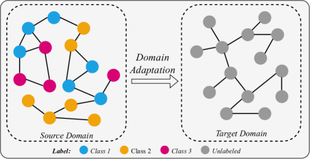
Figure 1. Illustration of graph domain adaptation. The source graph is all labeled and the target graph is unlabeled, domain adaptation aims to train a classifier in the source domain so as to transfer to the target domain classification.

In this paper, we address the aforementioned problems by formalizing a novel domain adaptive framework model named Spectral Augmentation for Graph Domain Adaptation (SA-GDA). Firstly, we find that the source and target domains share the feature space of labels, nodes with the same category but belonging to different domains present similar characters in the spectral domain, while different categories are quite distinct. Due to the scarcity of target labels, directly aligning the category feature space is difficult. As an alternative, with the observation above, we design a spectral augmentation submodule, which combines the target domain spectral information with the source domain to enhance the node representation learning, instead of aligning the whole feature space in the spatial domain. Besides, we theoretical analysis the bound of SA-GDA to guarantee the stability of the model. Then, considering that traditional GNN methods mainly focus on the aggregation of local information, ignoring the contribution of global information for node representation. We extract the local and global consistency of target domain to assist the node representation training. Lastly, we incorporate an adversarial scheme to effectively learn domain-invariant and semantic representations, thereby reducing the domain discrepancy for cross-domain node classification. Through extensive experiments, we demonstrate that our SA-GDA significantly outperforms state-of-the-art competitors. Our contribution can be summed up as follows:

• Under the graph domain adaptation settings, we have the observation that the spectral features of the same category in different domains present similar characteristics, while those of different categories are distinct.

• With the observation, we design the SA-GDA for node classification, which utilizes spectral augmentation to align the category features space instead of aligning the whole features space directly. Besides, we theoretical analyze the bound of SA-GDA to guarantee the stability of SA-GDA.

• Extensive experiments are conducted on real-world datasets, and the results show that our proposed SA-GDA outperforms the variety of state-of-the-art methods.

2. Related Work

2.1. Graph Neural Networks

Graph neural networks (GNNs) (Zhou et al., 2020) are designed to learn node embeddings in graph-structured data by mapping graph nodes with neighbor relationships to the low-dimensional latent space. Many approaches have been proposed to generalize the well-developed neural network models for regular grid structures, enabling them to utilize graph structured data for many downstream tasks, such as node classification and relationship prediction (Wu et al., 2020a; Yin and Luo, 2022), graph label noisy learning (Yin and Luo, 2022; Yin et al., 2023b). GCN (Kipf and Welling, 2017) integrates node features as well as graph topology on graph-structured data and exploits two graph convolutional layers for node classification tasks by semi-supervised learning. GAT (Veličković et al., 2018) enhances GCN in terms of message passing between nodes, using an attention mechanism to automatically integrate the features of the neighbors of a certain node. However, most existing GNN-based approaches focus on learning the node representation among a particular graph. When transferring the learned model between different graphs to perform the same downstream task, representation space drift and embedding distribution discrepancy may be encountered.

2.2. Unsupervised Domain Adaptation

Unsupervised domain adaptation is one of the transfer learning methods that aims to minimize the discrepancy between the source and target domains, thus transferring knowledge from the well-labeled source domain to the unlabeled target domain(Farahani et al., 2021; Sun et al., 2021a; Yin et al., 2023a, d). To perform cross-domain classification tasks, methods based on deep feature representation(Sun and Saenko, 2016), which map different domains into a common feature space, have attracted extensive attention. Most of these methods utilize adversarial training to reduce the inter-domain discrepancy(Long et al., 2015). Typically, DANN(Ganin et al., 2016a) utilizes a gradient reversal layer to capture domain invariant features, where the gradients are back-propagated from the domain classifier in a minimax game of the domain classifier and the feature extractor.

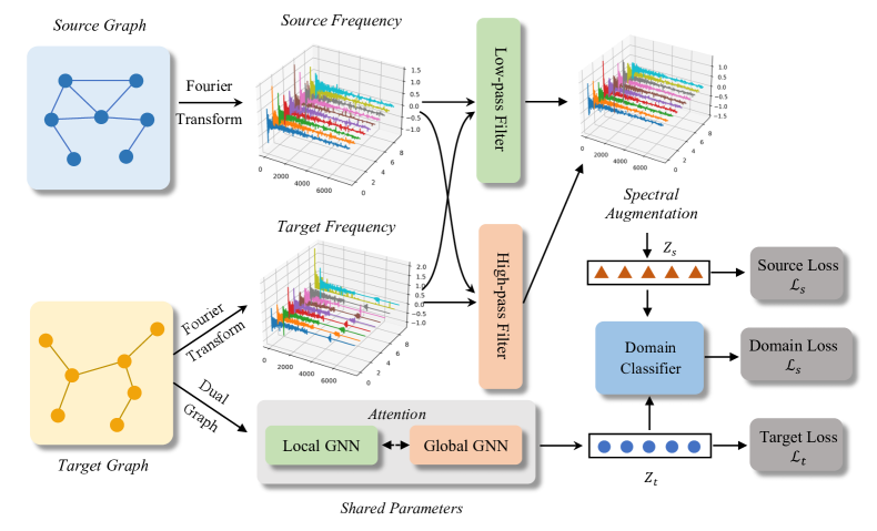
Figure 2. Overview of our proposed SA-GDA. SA-GDA first applies spectral augmentation to align the category feature space. Then a dual graph module learns the consistency representation from local and global perspectives. Last, we introduce three classifiers to learn the semantic representation for training source, domain, and target classifier.

Recently, for graph-structured data, several studies have been proposed for cross-graph knowledge transfer via unsupervised domain adaptation methods (Shen et al., 2020; Dai et al., 2019; Wu et al., 2020b; Yin et al., 2023a, 2022b). CDNE(Shen et al., 2020) learns transferable node representations through minimizing the maximum mean discrepancy (MMD) loss for cross-network learning tasks, yet cannot model the network topology. To enhance CDNE, AdaGCN(Dai et al., 2019) utilizes graph convolutional networks for feature extraction to learn the node representations, and then to learn domain-invariant node representations based on adversarial learning. UDA-GCN(Wu et al., 2020b) further models both local and global consistency information for cross-graph domain adaptation. DEAL (Yin et al., 2022b) and CoCo (Yin et al., 2023a) are designed for the classification of graph-level domain adaptation. However, most of the existing methods only align the feature space of the source and target domains, without considering the specific class alignment. Moreover, the unlabeled data are simply labeled based on pseudo-labeling. The above limitations may lead to the feature confusion among different categories in the target domain and the introduction of noise in the labels, which may negatively affect the model performance.

3. Methodology

3.1. Problem Definition

Graph Node Classification: Given a graph $G=(\mathcal{V},\mathcal{E},\bm{A},\bm{X},\bm{Y})$ with the set of nodes $\mathcal{V}$ and the set of edges $\mathcal{E}$. $\bm{A}\in\mathbb{R}^{N\times N}$ is the adjacency matrix of $G$, $\bm{D}$ is the degree matrix with $\bm{D}_{ii}=\sum_{j=0}^{N}{\bm{A}_{ij}}$ and $N$ denotes the number of nodes. The node feature denotes as $\bm{X}\in\mathbb{R}^{N\times d}$, where each row $\bm{x}_{v}\in\mathbb{R}^{d}$ represents the feature vector of node $v\in\mathcal{V}$ and $d$ is the dimension of node features. The normalized graph Laplacian matrix is defined $\bm{L}=\bm{I}-\bm{D}^{-\frac{1}{2}}\bm{AD}^{-\frac{1}{2}}$, $\bm{I}$ is the identity matrix. By factorization of $\bm{L}$, we have $\bm{L}=\bm{U}\bm{\Lambda U}^{\top}$, where $\bm{U}=[\bm{u_{1}},\cdots,\bm{u_{n}}]$, $\bm{\Lambda}=diag([\lambda_{1},\cdots,\lambda_{n}])$, $\bm{u_{i}}$ is the eigenvector and $\lambda_{i}$ is the corresponding eigenvalue. $\bm{Y}\in\mathbb{R}^{N\times C}$ is the label of $G$, $C$ is the number of classes.

Graph Domain Adaptation for Node Classification: Given the fully labeled source graph $G_{s}=(\mathcal{V}_{s},\mathcal{E}_{s},\bm{A}_{s},\bm{X}_{s},\bm{Y}_{s})$ and unlabeled target graph $G_{t}=(\mathcal{V}_{t},\mathcal{E}_{t},\bm{A}_{t},\bm{X}_{t})$, which shares the same label space $\mathcal{Y}=\{1,2,\cdots,C\}$ but distinct data distributions in the graph space, causing domain shifts. Our purpose is to train a classifier with the source $G_{s}$ and target $G_{t}$ for target node classification.

3.2. Overview

The two key difficulties of unsupervised domain adaptation for node classification are the challenging category alignment of graph data and the inefficient node classification with label scarcity. To tackle these challenges, we propose a novel model termed SA-GDA. Our proposed SA-GDA consists of a spectral augmentation module, a dual graph learning module, and a domain adversarial module. The spectral augmentation module combines the spectral features between source and target domain to implement the category feature alignment. The dual graph module aims to learn the consistency representation from local and global perspectives, and the domain adversarial module to differentiate the source and target domains.

3.3. Spectral Augmentation for Category Alignment

Domain adaptation methods in the past have typically used the pseudo-labeling mechanism (Zou et al., 2018; Liang et al., 2020) to align the feature space of categories. They involve assigning pseudo-labels to unlabeled data and using the labels to supervise the neural network. However, the risk of overconfidence and noise in these pseudo-labels would lead to potential biases during optimization and ultimately affect performance. Furthermore, in the graph domain, the lack of labels can worsen the noise issue.

Aligning the category feature space in the spatial domain is difficult due to the above problem. Inspired by the transductive learning method (Kipf and Welling, 2017), we try to explore the characteristics of categories with different domains in the spectral domain. Extracting the spectral features of nodes with the same category in the source and target domains, we find that they show a high degree of correlation, while the spectral features of different categories are distinct, which is shown in Figure 3.

With the observation, we design a spectral augmentation method for category alignment in the spectral domain instead of in the spatial domain. From the perspective of signal processing (Shuman et al., 2013), the graph Fourier is defined as $\bm{z}=\bm{U}^{\top}\bm{x}$, and the inverse Fourier transform is $\bm{x}=\bm{Uz}$. Then, the convolution on graph is: $f\star\bm{X}=\bm{U}((\bm{U}^{\top}f)\odot(\bm{U}^{\top}\bm{X}))=\bm{U}g_{\theta}\bm{U}^{\top}\bm{X},$ where $f$ is the convolution kernel, and $\odot$ is the element-wise product operation. Considering that low-frequency would lose the discrimination of node representation,  (Bo et al., 2021) utilize the attention to combine the low and high-frequency for node representation. In our work, we first apply the low-pass filter $g_{\theta}^{L}(\bm{\Lambda}_{d})$ and high-pass filter $g_{d}^{H}(\bm{\Lambda}_{d})$ to separate the low and high-frequency signals, where $d$ can be $s$ or $t$ for source and target domain. Denote $\bm{z}^{H}_{d}$ and $\bm{z}^{L}_{d}$ as the high and low-frequency signals of node representation $z$ on domain $d$, then:

(1) $$\bm{z}^{H}_{d}=\bm{U}_{d}g_{\theta}^{H}(\bm{\Lambda}_{d})\bm{U}_{d}^{\top}\bm{x},\quad\bm{z}^{L}_{d}=\bm{U}_{d}g_{\theta}^{L}(\bm{\Lambda}_{d})\bm{U}_{d}^{\top}\bm{x}.$$

Instead of aligning the category feature on the spatial domain, we combine the spectral domain information of source and target domain directly, because of the inhere naturally aligned spectral of the same category. Formally, in the source domain:

(2) $$\bm{Z}_{s}= \sigma(\bm{U}_{s}[\alpha g_{\theta}^{H}(\bm{\Lambda}_{s})\bm{U}_{s}^{\top}\bm{X}_{s}\bm{W}+(1-\alpha)g_{\theta}^{H}(\bm{\Lambda}_{t})\bm{U}_{t}^{\top}\bm{X}_{t}\bm{W}$$

$$+\beta g_{\theta}^{L}(\bm{\Lambda}_{s})\bm{U}_{s}^{\top}\bm{X}_{s}\bm{W}+(1-\beta)g_{\theta}^{L}(\bm{\Lambda}_{t})\bm{U}_{t}^{\top}\bm{X}_{t}\bm{W}]),$$

where $\alpha$ and $\beta$ are the hyperparameters for fusing high and low frequencies between source and target domain. $\bm{U}_{d}$ and $\bm{\Lambda}_{d}$ denotes the eigenmatrix and eigenvalue of domain $d$, and $d\in\{s,t\}$, $\sigma$ is the activation function and $\bm{W}$ is the trainable matrix.

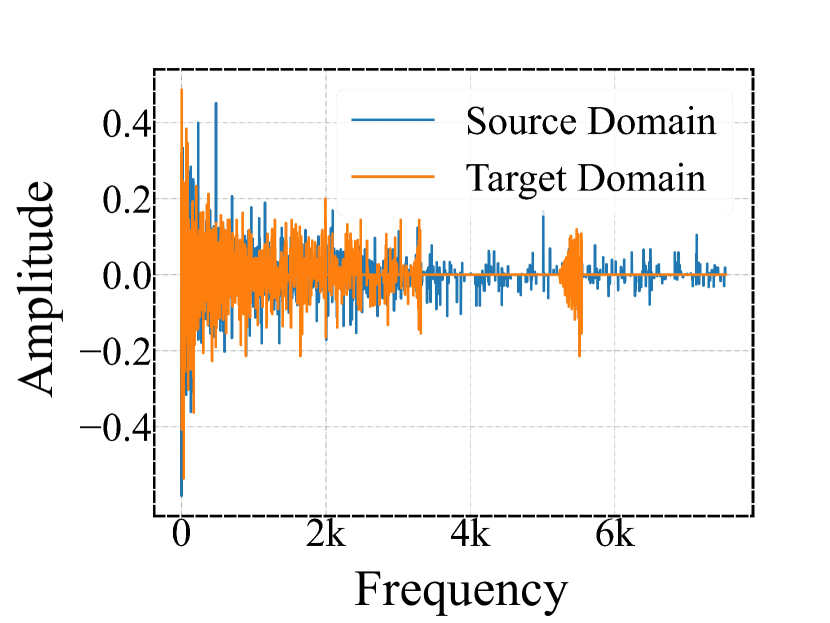
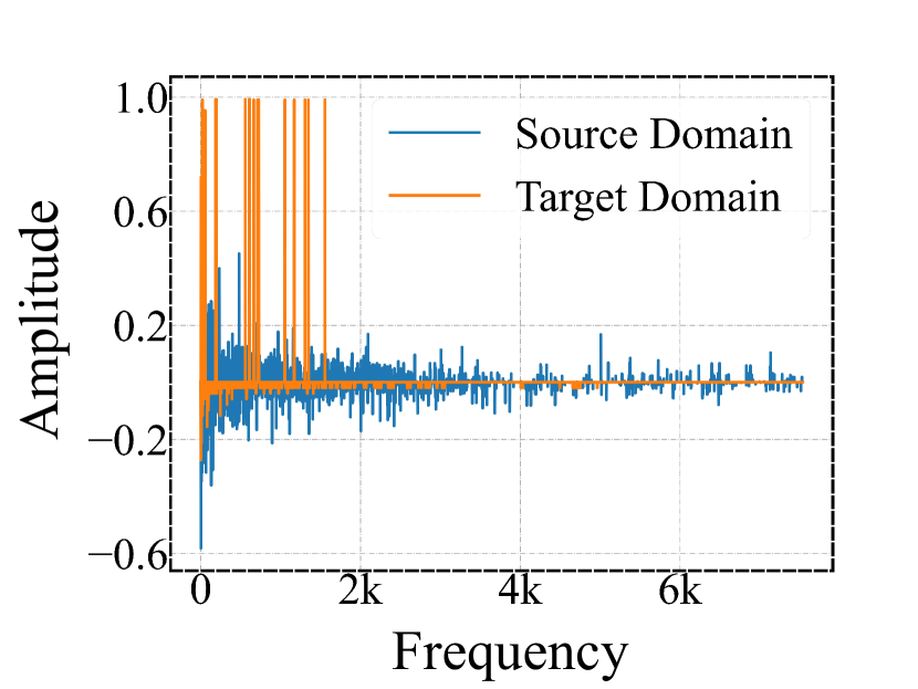
Figure 3. Left: The spectral of same category on different domains; Right: The spectral of different categories on different domains.

3.4. Attention-based Dual Graph Learning

To capture the local and global information of nodes, we propose a dual graph neural network, where the local consistency is extracted with the graph adjacency matrix and the global with the random walk GNN. Due to the source domain graph being fused with the target information from the global view, we apply dual graph learning on the target domain.

Local GNN. For the local consistency extraction, we use the GCN (Hamilton et al., 2017c) method directly. With the input $\bm{X}_{t}$ and adjacency matrix $\bm{A}_{t}$, the local node representation is defined as:

(3) $$\bm{Z}_{t,local}^{l}=\sigma(\tilde{\bm{D}}^{-\frac{1}{2}}\tilde{\bm{A}}\tilde{\bm{D}}^{-\frac{1}{2}}\bm{Z}_{t}^{l-1}\bm{W}^{l}),$$

where $\tilde{\bm{A}}=\bm{I}+\bm{A}_{t}$ is the adjacent matrix with self-loop, $\tilde{\bm{D}}_{ii}=\sum_{j}\tilde{\bm{A}}_{ij}$, $\bm{W}^{l}$ is the trainable matrix on the $l$-th layer. $\bm{Z}_{t}^{l}$ is the node embeddings of target domain on the $l$-th layer and $\bm{Z}_{t}^{0}=\bm{X}_{t}$.

Global GNN. To achieve global information, similar to (Wu et al., 2020b), we apply the random walk to calculate the semantic similarities between nodes and calculate the global consistency with the newly constructed adjacency matrix.

Define the state of node $v_{i}$ at time $t$ as $s(t)=v_{i}$. The transition probability of jumping $v_{i}$ to the neighbors $v_{j}$ is defined as:

(4) $$\bm{P}_{ij}=p(s(t+1)=v_{j}|s(t)=v_{i})=\frac{\bm{A}_{t(ij)}}{\sum_{j}\bm{A}_{t(ij)}},$$

where $\bm{A}_{t(ij)}$ denotes the value of $\bm{A}_{ij}$ on the target domain. Then, we calculate the point-wise mutual information matrix (Klabunde, 2002) as:

(5) $$\bm{M}_{ij}=max\{log(\frac{m_{ij}}{m_{i\star}m_{\star j}}),0\},$$

where $m_{ij}=\frac{\bm{P}_{ij}}{\sum_{i,j}\bm{P}_{ij}}$, $m_{i\star}=\frac{\sum_{j}\bm{P}_{ij}}{\sum_{i,j}\bm{P}_{ij}}$ and $m_{\star j}=\frac{\sum_{i}\bm{P}_{ij}}{\sum_{i,j}\bm{P}_{ij}}$.

With the calculated adjacency matrix $\bm{M}$, we extract the global node information as follows:

(6) $$\bm{Z}_{t,global}^{l}=\sigma(\bm{D}^{-\frac{1}{2}}\bm{M}\bm{D}^{-\frac{1}{2}}\bm{Z}_{t}^{l-1}\bm{W}^{l}),$$

where $\bm{D}_{ii}=\sum_{j}\bm{M}_{ij}$, and $\bm{W}^{l}$ is the shared parameters with Eq. 3.

Attention-based fusion. To fuse the local and global information, we utilize the attention mechanism $a:\mathbb{R}^{d^{\prime}}\times\mathbb{R}^{d^{\prime}}\to\mathbb{R}$ to computer the attention coefficients:

$$e_{ij} =a(\bm{Wz}_{i,local},\bm{Wz}_{j,global}),$$

$$\zeta_{ij}= softmax(e_{ij})=\frac{exp(e_{ij})}{\sum_{k}exp(e_{ij})},$$

where $\bm{W}\in\mathbb{R}^{d^{\prime}\times d}$ is the shared matrix, and we choose $a(\bm{h}_{i},\bm{h}_{j})=LeakyReLu(\bm{W}_{0}^{\top}[\bm{Wh}_{i}||\bm{Wh}_{j}])$ with learnable matrix $\bm{W}_{0}\in\mathbb{R}^{2d^{\prime}}$ and $||$ denotes concatenation operation. The fused representation of local and global is calculated as:

(7) $$\bm{Z}_{t}=\zeta_{ii}\bm{Z}_{t,local}+(1-\zeta_{ii})\bm{Z}_{t,global}.$$

3.5. Domain Adversarial Training

The spectral augmentation of the category alignment module enforces the similarity of features across different domains, confusing source and target domain features. Our goal is to maximize the domain classification error while minimizing the source domain classification error, i.e.,

(8) $$\mathop{min}\limits_{\theta_{y}}\mathop{max}\limits_{\theta_{d}}=\mathcal{L}_{s}(f(\bm{z}_{s};\theta_{y}))-\gamma\mathcal{L}_{D}(h(\bm{z};\theta_{d})),$$

where $f(\bm{z}_{s};\theta_{y})=softmax(\theta_{y}\bm{z}_{s})$ is the source classification function, and $\theta_{y}$ is the trainable parameters for $f$. $h(\bm{z};\theta_{d})=sigmod(\theta_{d}\bm{z})$ is the domain classifier, $\theta_{d}$ is the parameters for $h$. $\mathcal{L}_{s}$ and $\mathcal{L}_{D}$ are the source classification loss and domain classification loss. $\bm{z}_{s}$ denotes the source features and $\bm{z}$ denotes the features of the source and target domains.

3.6. Optimization

Our SA-GDA has the overarching goal that combines the domain adversarial loss and classification loss of the target data. Additionally, minimizing the expected source error for labeled source samples is also essential. In formation,

(9) $$\mathop{min}\limits_{\theta_{y}}\mathop{max}\limits_{\theta_{d}}\mathcal{L}(\theta_{y},\theta_{d})= \mathcal{L}_{s}(f(\bm{z}_{s};\theta_{y}))+\gamma_{1}\mathcal{L}_{t}(f(\bm{z}_{t};\theta_{y}))$$

$$-\gamma_{2}\mathcal{L}_{D}((h(\bm{z};\theta_{d})),$$

with the source loss $\mathcal{L}_{s}$, target loss $\mathcal{L}_{t}$ and domain loss $\mathcal{L}_{D}$:

$$\mathcal{L}_{s}=- \frac{1}{N_{s}}\sum_{i=1}^{N_{s}}y_{i}log(f(\bm{z}_{s})),$$

$$\mathcal{L}_{t}=- \frac{1}{N_{t}}\sum_{i=1}^{N_{t}}f(\bm{z}_{t})log(f(\bm{z}_{t})),$$

$$\mathcal{L}_{D}=-\frac{1}{N_{s}+N_{t}} \sum_{i=1}^{N_{s}+N_{t}}d_{i}log\frac{1}{h(\bm{z})}+(1-d_{i})log\frac{1}{1-h(\bm{z})},$$

where $\gamma_{1}$ and $\gamma_{2}$ are hyper-parameters to balance the domain adversarial loss and target classification loss. $d_{i}\in\{0,1\}$ denotes node $i$ belongs to the source or target domain. To update the parameters of Eq. 9 in the standard stochastic gradient descent (SGD) method, we apply the Gradient Reversal Layer (Ganin et al., 2016a) (GRL) $\mathcal{R}$ for model training, which is formulate as:

(10) $$\mathcal{R}(\bm{x})=\bm{x},\quad\frac{d\mathcal{R}}{d\bm{x}}=-\bm{I}.$$

Then, the update of Eq. 9 can be implemented with SGD with the following formulation:

(11) $$\mathop{min}\limits_{\theta_{y},\theta_{d}}\mathcal{L}(\theta_{y},\theta_{d})= \mathcal{L}_{s}(f(\mathcal{R}(\bm{z}_{s});\theta_{y}))+\gamma_{1}\mathcal{L}_{t}(f(\mathcal{R}(\bm{z}_{t});\theta_{y}))$$

$$-\gamma_{2}\mathcal{L}_{D}((h(\mathcal{R}(\bm{z});\theta_{d})).$$

The whole learning procedure is shown in Algorithm 1.

Algorithm 1 Training Algorithm of SA-GDA

0:  Source domain adjacency matrix $A_{s}$, degree matrix $D_{s}$; target domain adjacency matrix $A_{t}$, degree matrix $D_{t}$, updating steps $E$;  

0:  Parameters $\theta$ for the neural network;

1:  Initialize $\theta$;

2:  Transform the source and target spatial graph features into spectral domain.

3:  for $e=1,2,\cdots,E$ do

4:     Calculate the spectral augmentation features on the source domain $Z_{s}$ with Eq. 2;

5:     Calculate the local and global features with dual graph on the target domain $Z_{t}$ with Eq. 3.4;

6:     Update the network parameters $\theta$ through backpropagation by Eq. 11;

7:  end for

3.7. Theoretical Analysis

In this subsection, we proof the stability of SA-GDA, which is inspired by (You et al., 2023):

Lemma 0.

Suppose the $G_{s}$ and $G_{t}$ are the graphs of the source and target domain. Given the Laplace matrices decomposition $\bm{L}_{d}=\bm{D}_{d}-\bm{A}_{d}=\bm{U}_{d}\bm{\Lambda}_{d}\bm{U}_{d}^{\top}$, where $\bm{\Lambda}_{d}=diag[\lambda_{d1},\cdots,\lambda_{dn}]$ are the sorted eigenvalues of $L_{d}$, and $d\in\{s,d\}$ denotes the source and target domains. The GNN is constructed as $f(G)=\sigma((g_{\theta}(\bm{L})\bm{XW})=\sigma(\bm{U}g_{\theta}(\bm{\Lambda})\bm{U}^{\top}\bm{XW})$, where $g_{\theta}$ is the polynomial function with $g_{\theta}(\bm{L})=\sum_{k=0}^{K}\theta_{k}\bm{L}^{k}$, $\bm{W}$ is the learnable matrix and the pointwise nonlinearity has $|\sigma(b)-\sigma(a)|\leq|b-a|$. Assuming $||\bm{X}||_{op}\leq 1$ and $||\bm{W}||_{op}\leq 1$, we have the following inequality:

(12) $$||f(G_{s}+G_{t})-f(G_{t})||_{2}\leq \alpha[C_{\lambda}(1+\tau)||\bm{L}_{s}-\bm{P}^{\star}\bm{L}_{t}\bm{P}^{\star\top}||_{F}$$

$$+\mathcal{O}(||\bm{L}_{s}-\bm{P}^{\star}\bm{L}_{t}\bm{P}^{\star\top}||_{F}^{2})$$

$$+max(|g_{\theta}(\bm{L}_{t})|)||\bm{X}_{s}-\bm{P}^{\star}\bm{X}_{t}||_{F}],$$

where $\tau=(||\bm{U}_{s}-\bm{U}_{t}||_{F}+1)^{2}-1$ stands for the eigenvector misalignment which can be bounded. $\Pi$ is the set of permutation matrices, and $\bm{P}^{\star}=argmin_{\bm{P}\in\Pi}{||\bm{X}_{s}-\bm{PX}_{t}||_{F}+||\bm{A}_{s}-\bm{PA}_{t}\bm{P}^{\top}||_{F}}$. $\mathcal{O}(||\bm{L}_{s}-\bm{P}^{\star}\bm{L}_{t}\bm{P}^{\star\top}||_{F}^{2}$ is the remainder term with bounded multipliers defined in (Gama et al., 2020), and $C_{\lambda}$ is the spectral Lipschitz constant that $\forall\lambda_{i},\lambda_{j},|g_{\theta}(\lambda_{i})-g\theta(\lambda_{j})|\leq C_{\lambda}(\lambda_{i}-\lambda_{j})$.

Table 1. The specific statistics of the experimental datasets.

Dataset	#Nodes	#Edges	#Features	#Labels
DBLPv7	5484	8130	6775	6
ACMv9	9360	15602	6775	6
Citationv1	8935	15113	6775	6

4. Experiment

In this section, we conduct extensive experiments on various real-world datasets to verify the effectiveness of the proposed SA-GDA. We aim to answer the questions below:

• RQ1: How does the proposed SA-GDA perform compared with the state-of-the-art baseline methods for node classification?

• RQ2: How is the effectiveness of proposed components on the performance?

• RQ3: How does the hyper-parameters affect the performance of the proposed SA-GDA?

• RQ4: How about the intuitive effect of proposed SA-GDA?

Table 2. Classification accuracy comparisons on six cross-domain tasks.

Methods	C$\to$D	A$\to$D	D$\to$C	A$\to$C	D$\to$A	C$\to$A	average
DeepWalk(Perozzi et al., 2014)	0.1222	0.2308	0.2210	0.2660	0.1437	0.2144	0.1997
LINE(Tang et al., 2015)	0.1938	0.2604	0.1976	0.3317	0.1576	0.2027	0.2240
GraphSAGE(Hamilton et al., 2017b)	0.5487	0.4443	0.4860	0.5043	0.5749	0.4794	0.5063
DNN(Montavon et al., 2018)	0.3699	0.3656	0.3913	0.4407	0.3363	0.4059	0.3850
GCN(Kipf and Welling, 2017)	0.5467	0.4392	0.4871	0.5039	0.5184	0.4785	0.4956
DGC(Wang et al., 2021)	0.5587	0.4589	0.5178	0.5250	0.5298	0.4890	0.5132
SUBLIME(Liu et al., 2022)	0.5650	0.4699	0.5012	0.5392	0.5247	0.5220	0.5203
DGRL(Ganin et al., 2016b)	0.3699	0.3756	0.3905	0.4514	0.3439	0.4063	0.3896
AdaGCN(Sun et al., 2021b)	0.5516	0.4470	0.4872	0.5094	0.5752	0.4884	0.5098
UDA-GCN(Wu et al., 2020b)	0.6599	0.4710	0.5809	0.5229	0.5959	0.5498	0.5634
SA-GDA(ours)	0.7097	0.6444	0.6460	0.6420	0.6296	0.6136	0.6476

4.1. Benchmark Datasets

To evaluate the effectiveness of the proposed SA-GDA, we have developed three citation networks from ArnetMiner(Tang et al., 2008), including DBLPv7, ACMv9, and Citationv1. These datasets are derived from different data sources (DBLP, ACM and Microsoft Academic Graph) and distinct time periods. Each sample contains a title, an index, a category and a citation index, where the category represents the academic field, including ”Artificial intelligence”, ”Computer vision”, ”Database”, ”Data mining”, ”High Performance Computing” and ”Information Security”. Following (Wu et al., [n. d.]), these datasets are constructed as undirected citation networks, where a node represents a paper, an edge indicates a citation record, and a label indicates the paper category. Since these three graphs are generated from different data sources and time periods, their distributions are naturally diverse. Thus, we can conduct six cross-domain node classification tasks (source$\to$target), including C$\to$D, A$\to$D, D$\to$C, A$\to$C, D$\to$A, and C$\to$A, where D, A, C denote DBLPv7, ACMv9, and Citationv1, respectively. The statics of these datasets is shown in Table 1.

4.2. Baselines

To verify the effectiveness of our method, we select the following methods as baselines for comparison, including seven state-of-the-art single-domain node classification methods (i.e., DeepWalk(Perozzi et al., 2014), LINE(Tang et al., 2015), GraphSAGE(Hamilton et al., 2017b), DNN(Montavon et al., 2018), GCN(Kipf and Welling, 2017), DGC(Wang et al., 2021), and
SUBLIME(Liu et al., 2022)), and three cross-domain classification methods with domain adaptation (i.e., DGRL(Ganin et al., 2016b), AdaGCN(Sun et al., 2021b) and UDA-GCN(Wu et al., 2020b)).

Single-domain node classification methods:

• DeepWalk(Perozzi et al., 2014): DeepWalk employs the random walk sampling strategy to capture the neighborhood node structure. Then, following Skip-Gram(Guthrie et al., 2006), which aims to learn the low-dimensional node representation on single domain.

• LINE(Tang et al., 2015): LINE is a classic method for large-scale graph representation learning, which preserves both first and second-order proximities for undirected network to measure the relationships between two nodes. Compared with the deep model, LINE has a limited representation ability.

• GraphSAGE(Hamilton et al., 2017b): GraphSAGE learns the node representation by aggregating the sampled neighbors for final prediction.

• DNN(Montavon et al., 2018): DNN is a multi-layer perceptron (MLP) based method, which only leverages node features for node classification.

• GCN(Kipf and Welling, 2017): GCN is a deep convolutional network on graphs, which employs the symmetric-normalized aggregation method to learn the embedding for each node.

• DGC(Wang et al., 2021): DGC is a linear variant of GCN, which separates the feature propagation steps from the terminal time, enhancing flexibility and enabling it to utilize a vast range of feature propagation steps.

• SUBLIME(Liu et al., 2022): SUBLIME generates an anchor graph from the raw data and uses the contrastive loss to optimize the consistency between the anchor graph and the learning graph, thus tackling the unsupervised graph structure learning problem.

Cross-domain node classification methods:

• DGRL(Ganin et al., 2016b): DGRL employs a 2-layer perceptron to extra feature and a gradient reverse layer (GRL) to learn node embedding for domain classification.

• AdaGCN(Sun et al., 2021b): AdaGCN uses a GCN as the feature extractor and a gradient reverse layer(GRL) to train a domain classifier.

• UDA-GCN(Wu et al., 2020b): UDA-GCN utilizes a dual graph convolutional network to preserve both local and global consistency information for generating better node embedding features through the attention mechanism. Also, a gradient reverse layer(GRL) is added to train a domain classifier.

Table 3. Classification accuracy comparisons between SA-GDA variants on six cross-domain tasks.

Methods	C$\to$D	A$\to$D	D$\to$C	A$\to$C	D$\to$A	C$\to$A	average
SA-GDA$\neg l$	0.3307	0.3298	0.3047	0.2612	0.2958	0.2694	0.2986
SA-GDA$\neg h$	0.6685	0.5746	0.5795	0.5449	0.5620	0.5345	0.5773
SA-GDA$\neg p$	0.5694	0.4659	0.5071	0.5259	0.5401	0.4998	0.5180
SA-GDA$\neg d$	0.6982	0.5997	0.6321	0.5747	0.5259	0.5567	0.5979
SA-GDA$\neg t$	0.6657	0.5915	0.5871	0.5264	0.5601	0.5289	0.5766
SA-GDA	0.7097	0.6444	0.6460	0.6420	0.6296	0.6136	0.6476

4.3. Experimental Settings

We utilize PyTorch (Paszke et al., 2017) and PyTorch Geometric library (Fey and Lenssen, 2019) as the deep-learning Framework and Adam (Kingma and Ba, 2015) as an optimizer. We follow the principles of evaluation protocols used in unsupervised domain adaptation to perform a grid study of all methods in the hyperparameter space and show the best results obtained for each method. To be fair, for all the cross-domain node classification methods in this experiment, we use the same parameter settings, except for some special cases. For each method, we set the learning rate to $1e^{-4}$. For the specific GCN-based models (e.g., GCN, DGC, SUBLIME, AdaGCN, and UDA-GCN), the number of hidden layers is set to 2, and the hidden dimensions are set to 128 and 16 regardless of the source and target domains. We use the same settings as above for both the local and global GNN. For DeepWalk and LINE, we first learn node embeddings and then train node classifiers using information from source domain, the hidden dimension of the node embeddings is set to 128. For DNN and DGRL, we set the same hidden dimensions as GNN-based models. The balance parameters $\gamma_{1}$, $\gamma_{2}$ are set to 0.3 and 0.1, and the dropout rate for each layer of dual GNN to 0.3. For simplicity, we set the combination weight of high and low-frequency as the same, i.e., $\alpha=\beta$.

4.4. Performance Comparison (RQ1)

We present the performance of SA-GDA compared with baselines under the setting of graph domain adaptation for node classification to answer RQ1, which is shown in Table 2. From the results:

• DeepWalk and LINE achieve the worst performance among all the methods, this is because they only utilize the network topology to generate node embedding without exploiting the node feature information. DNN also achieves a poor performance, contrary to the above two methods, it only considers the node features and ignores the association between nodes, so it cannot generate better node embeddings.

• The graph-based methods (GCN, GraphSAGE, DGC, and SUBLIME) outperform DeepWalk and LINE, we attribute the reason to that they encode both local graph structure and node features to obtain better node embeddings.

• DGRL, AdaGCN, and UDA-GCN achieve better performance than the single-domain node classification methods. The reason is that, by incorporating the domain adversarial learning, the node classifier is capable to transfer the knowledge from the source to the target domain.

• The proposed SA-GDA model achieves the best performance in these six cross-domain node classification datasets compared to all the baseline methods. By fusing the low and high-frequency signals of different domains in the spectral domain, SA-GDA implements the category alignment under the domain-variant setting. This enables us to learn better graph node embeddings and to train node classifiers in both the source and target domains through an adversarial approach, which greatly reduces the distribution discrepancies between the different domains and improves the node classifier performance.

4.5. Ablation Study (RQ2)

To answer RQ2, we introduce several variants of the SA-GDA to investigate the effectiveness of each component of SA-GDA:

• SA-GDA$\neg l$, which evaluates the impact of low-frequency signals in both source and target domains.

• SA-GDA$\neg h$, evaluating the influence of high-frequency signals in different domains.

• SA-GDA$\neg p$, which remove the global GNN and utilizing only the local GNN.

• SA-GDA$\neg d$, which removes the domain loss to evaluate the impact of domain adversarial learning.

• SA-GDA$\neg t$, which evaluate the effectiveness of target classifier by removing the target loss.

The results are reported in Table 3, and we have the following observation:

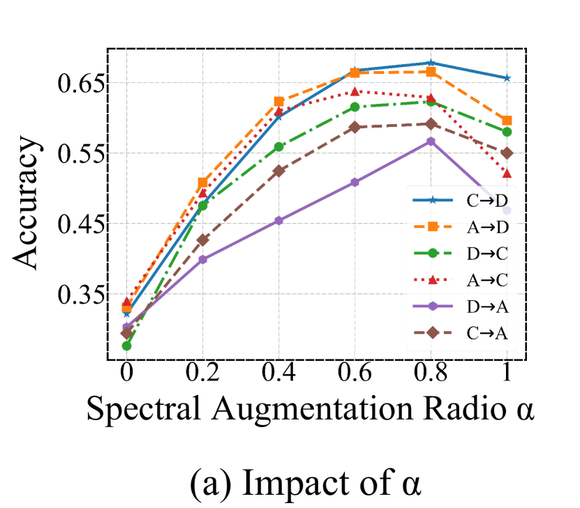
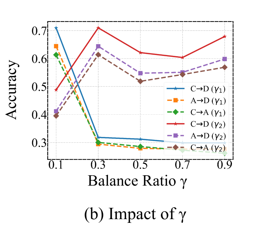
Figure 4. Sensitivity analysis on different tasks.

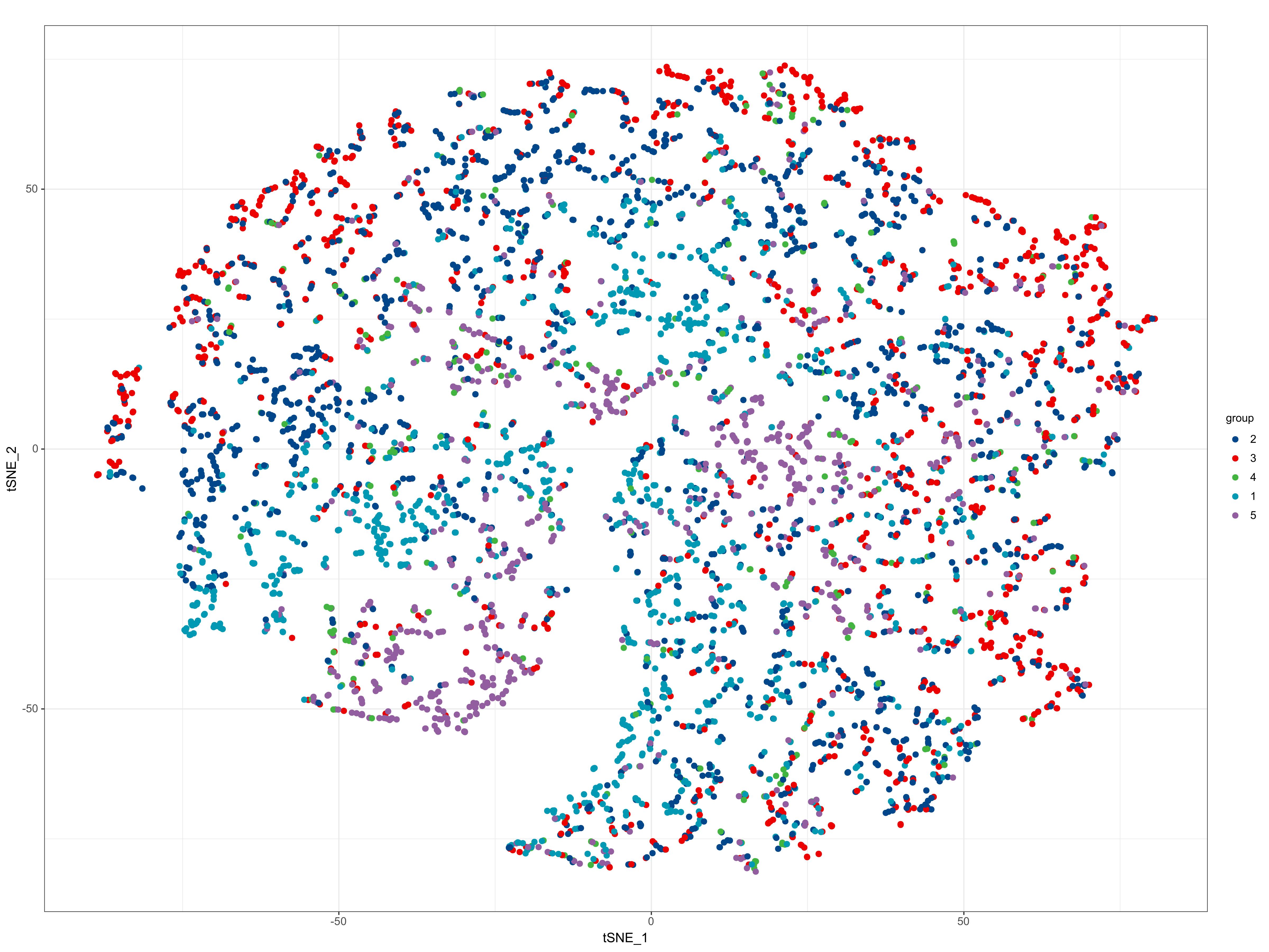
(a) DNN

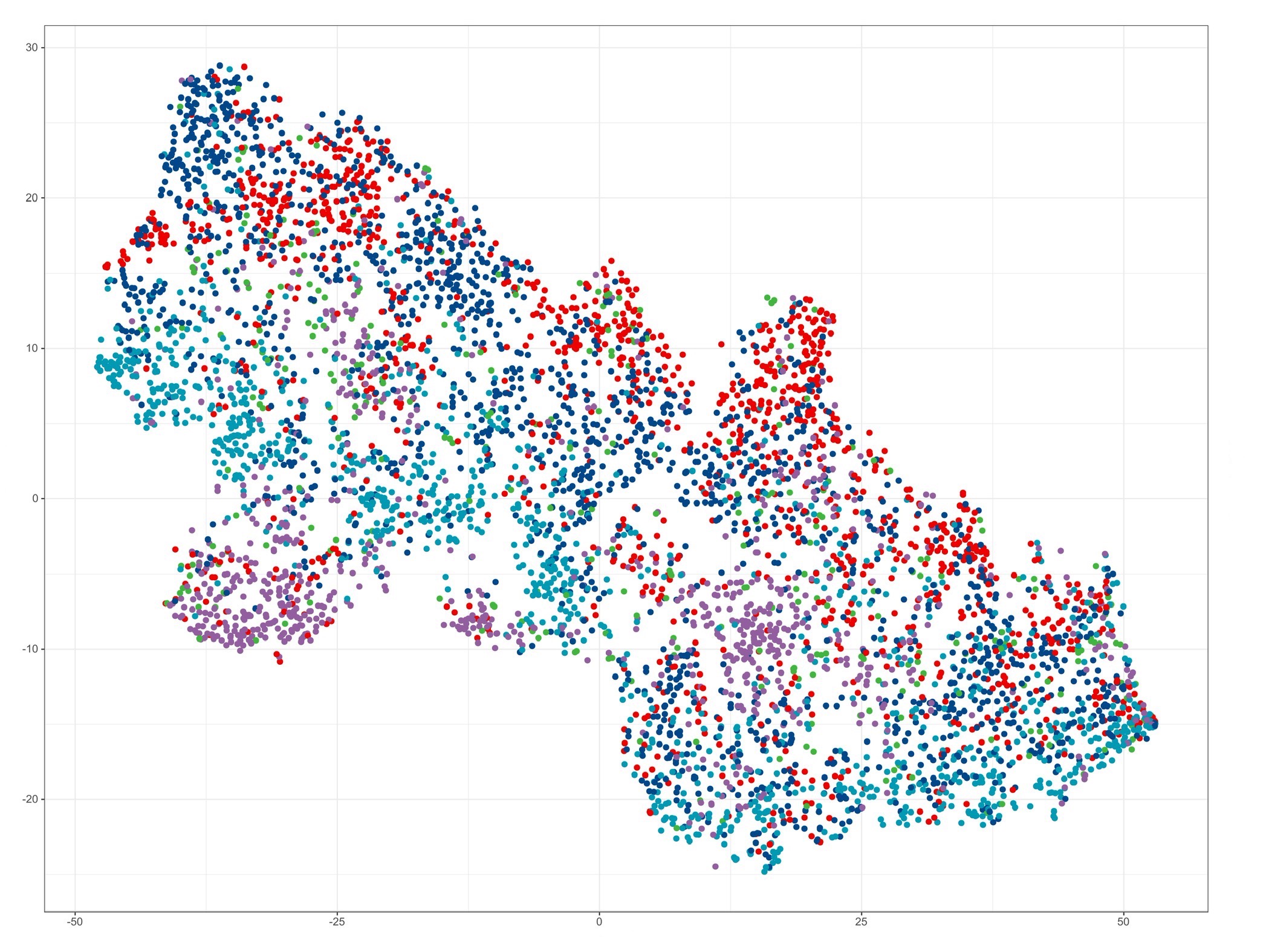
(b) GraphSAGE

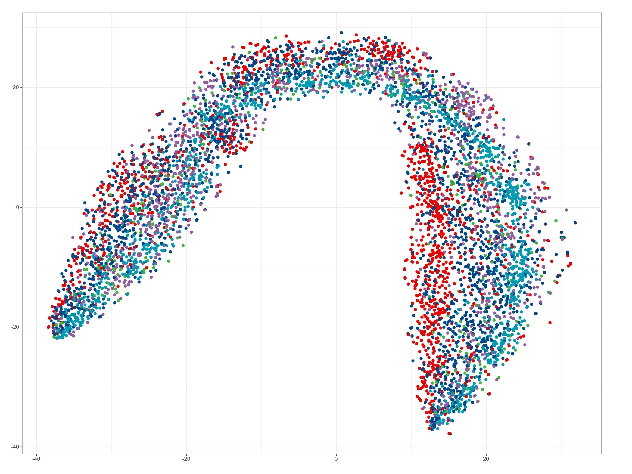
(c) UDA-GCN

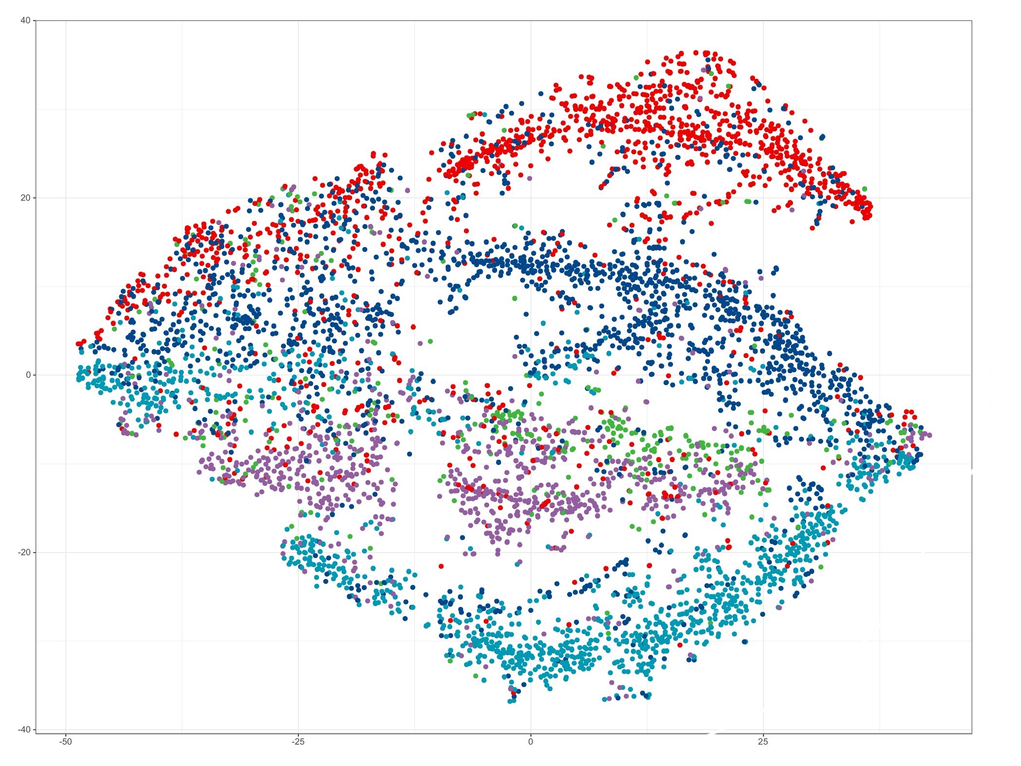
(d) SA-GDA

Figure 5. Visualization of the embedding features learned from different methods using $t$-SNE.

• Impact of Low-frequency Signals: To justify the importance of low-frequency signals in spectral domain, we compare the variant model SA-GDA$\neg l$ with the original model SA-GDA. As shown in Table 3, we can evidently observe that the performance of the original model in all tasks are substantially enhanced compared with SA-GDA$\neg l$. This indicates that the combination of low-frequency signals from both domains greatly reduces the category discrepancy between domains and contributes significantly to the cross-domain graph node classification accuracy.

• Impact of High-frequency Signals: To present the impact of high-frequency signals in spectral augmentation, we compare the proposed model SA-GDA with SA-GDA$\neg h$. Through Table 3, we find that the performance of SA-GDA in all tasks are suitably improved compared to SA-GDA$\neg h$. Although the contribution of combining high-frequency signals in both domains is limited compared to the low-frequency signals, but it is still effective for the cross-domain node classification tasks.

• Impact of Global GNN: To verify the effectiveness of the global consistency information extractor in dual GNN module, we compare SA-GDA with SA-GDA$\neg p$. Through the results, we observe that the performance of SA-GDA is better than SA-GDA$\neg p$, indicating that the global information would help to improve the representation ability in dual GNN, thus achieving better results.

• Impact of Domain Adversarial Training: To evaluate the effectiveness of domain adversarial training module, we compare SA-GDA with SA-GDA$\neg d$. In Table 3, the performance of SA-GDA is improved by a certain magnitude compared with SA-GDA$\neg d$, we contribute the reason to that the presence of domain classifier would reduce the discrepancy between source and target domains, thus increasing the accuracy of the target domain.

• Impact of the Target Loss: From Table 3, we can find that the proposed model SA-GDA performs to a certain extent higher than SA-GDA$\neg t$ in all six cross-domain node classification tasks, which indicates that the target domain classifier loss is a critical information in the cross-domain problem.

4.6. Sensitivity Analysis (RQ3)

To answer RQ3, we conduct experiments to evaluate how the hyper-parameters $\alpha$, $\beta$ and $\gamma_{1}$, $\gamma_{2}$ affect the performance of proposed SA-GDA. $\alpha$ and $\beta$ control how much of the high and low-frequency combined in the spectral augmentation module, and $\gamma_{1}$, $\gamma_{2}$ control the balance of target classification and domain adversarial loss. In the implementation, we set $\alpha=\beta$ and vary $\alpha$ in $\{0,0.2,0.4,0.6,0.8,1\}$ with other parameters fixed. Besides, we set $\gamma_{1}$ and $\gamma_{2}$ in $\{0.1,0.3,0.5,0.7,0.9\}$ respectively. The results is shown in Fig. 4, from the results, we have the following observation:

• Impact of Spectral Augmentation Ratio $\alpha$: Fig. 4(a) shows the impact of $\alpha$, we observe that the classification accuracy improves gradually when $\alpha$ changes from 0 to 0.8, while decrease when $\alpha$ ranges in $\{0.8,1\}$. This is because SA-GDA needs more spectral information from the source domain for training, while if $\alpha$ is too large, the effectiveness of the spectral augmentation would be weakened, resulting the poor performance. Hence, we set $\alpha$ to 0.8 in our implementation.

• Impact of Balance Ratio $\gamma_{1}$ and $\gamma_{2}$: We conduct a large number of experiments by setting $\gamma_{1}$ and $\gamma_{2}$ in $\{0.1,0.3,0.5,0.7,0.9\}$ respectively, and report the best results as shown in Fig. 4(b). From Fig. 4(b), we find that, when $\gamma_{2}$ fixed at 0.1, the performance tends to increase first and then decrease in most cases. The reason is that a small $\gamma_{1}$ would incorporate the target information for classification while a large $\gamma_{1}$ may introduce more uncertain information for the scarcity of target labels. Thus, we set $\gamma_{1}$ to 0.3 as default. Similar to $\gamma_{1}$, we change the value of $\gamma_{2}$ with $\gamma_{1}$ fixed to 0.3. We observe that increasing $\gamma_{2}$ results in better performance when it is small, indicating that the domain classifier would help to improve the accuracy. However, too large $\gamma_{2}$ may hurt the performance, which demonstrates that too large of domain loss could harm the discrimination information. Thus, we set $\gamma_{2}$ to 0.1 as default.

4.7. Visualization (RQ4)

In order to achieve an intuitive effect of proposed SA-GDA, we visualize the node representation learned in the target domain to answer RQ4. We visualize the Citationv1$\to$DBLPv7 task and compare it with three models (DNN, GraphSAGE and UDA-GCN), and we have the similar observation on other datasets. In particular, for each method, we represent the node embeddings with the Stochastic Neighbor Embedding ($t$-SNE) (Laurens and Hinton, 2008) method, and the results is shown in Fig. 5. From Fig. 5, we observe that the visualization results of DNN do not have a clear expressive meaning due to the absence of a large number of similar nodes clustered together and the obvious overlap between classes. Compared with DNN, GraphSAGE and UDA-GCN achieve better visualization representation and the relationship between classes becomes clearer. However, the problem of unclear clustering boundaries still exists. In the visual representation of our proposed SA-GDA, the clustering results are clearer compared to the above methods. Meanwhile, there are more obvious boundaries between classes, which indicates that SA-GDA can generate more meaningful node representation.

5. Conclusion

In this paper, we study a less-explored problem of unsupervised domain adaptation for graph node classification and propose a novel framework SA-GDA to solve the problem. First, we find the inherent features of same category in different domains, i.e., the correlation of nodes with same category is high in spectral domain, while different categories are distinct. Following the observation, we apply spectral augmentation for category alignment instead of whole feature space alignment. Second, the dual graph extract the local and global information of graphs to learn a better representation for nodes. Last, by using the domain adversarial learning cooperating with source and target classification loss, we are able to reduce the domain discrepancy and achieve the domain adaptation. We conduct extensive experiments on real-world datasets, the results show that our proposed SA-GDA outperforms the existing cross domain node classification methods. Although the proposed SA-GDA has achieved impressive results, the complexity of matrix decomposition is high. In the future, we will explore more efficient spectral domain alignment methods and utilize spatial domain features to assist the alignment of category features in different domains, thereby reducing the model complexity.

6. acknowledge

This work was supported by the National Key R&D Program of China under Grant No. 2020AAA0108600.

Appendix A Theoretical Analysis

In this subsection, we proof the stability of SA-GDA, which is inspired by (You et al., 2023):

Lemma 0.

Suppose the $G_{s}$ and $G_{t}$ are the graphs of the source and target domain. Given the Laplace matrices decomposition $\bm{L}_{d}=\bm{D}_{d}-\bm{A}_{d}=\bm{U}_{d}\bm{\Lambda}_{d}\bm{U}_{d}^{\top}$, where $\bm{\Lambda}_{d}=diag[\lambda_{d1},\cdots,\lambda_{dn}]$ are the sorted eigenvalues of $L_{d}$, and $d\in\{s,d\}$ denotes the source and target domains. The GNN is constructed as $f(G)=\sigma((g_{\theta}(\bm{L})\bm{XW})=\sigma(\bm{U}g_{\theta}(\bm{\Lambda})\bm{U}^{\top}\bm{XW})$, where $g_{\theta}$ is the polynomial function with $g_{\theta}(\bm{L})=\sum_{k=0}^{K}\theta_{k}\bm{L}^{k}$, $\bm{W}$ is the learnable matrix and the pointwise nonlinearity has $|\sigma(b)-\sigma(a)|\leq|b-a|$. Assuming $||\bm{X}||_{op}\leq 1$ and $||\bm{W}||_{op}\leq 1$, we have the following inequality:

(13) $$||f(G_{s}+G_{t})-f(G_{t})||_{2}\leq \alpha[C_{\lambda}(1+\tau)||\bm{L}_{s}-\bm{P}^{\star}\bm{L}_{t}\bm{P}^{\star\top}||_{F}$$

$$+\mathcal{O}(||\bm{L}_{s}-\bm{P}^{\star}\bm{L}_{t}\bm{P}^{\star\top}||_{F}^{2})$$

$$+max(|g_{\theta}(\bm{L}_{t})|)||\bm{X}_{s}-\bm{P}^{\star}\bm{X}_{t}||_{F}],$$

where $\tau=(||\bm{U}_{s}-\bm{U}_{t}||_{F}+1)^{2}-1$ stands for the eigenvector misalignment which can be bounded. $\Pi$ is the set of permutation matrices, and $\bm{P}^{\star}=argmin_{\bm{P}\in\Pi}{||\bm{X}_{s}-\bm{PX}_{t}||_{F}+||\bm{A}_{s}-\bm{PA}_{t}\bm{P}^{\top}||_{F}}$. $\mathcal{O}(||\bm{L}_{s}-\bm{P}^{\star}\bm{L}_{t}\bm{P}^{\star\top}||_{F}^{2}$ is the remainder term with bounded multipliers defined in (Gama et al., 2020), and $C_{\lambda}$ is the spectral Lipschitz constant that $\forall\lambda_{i},\lambda_{j},|g_{\theta}(\lambda_{i})-g\theta(\lambda_{j})|\leq C_{\lambda}(\lambda_{i}-\lambda_{j})$.

Proof. Similar to (You et al., 2023), we use $\bm{P}^{\star}$ as the optimal permutation matrix for $G_{s}$ and $G_{t}$. With Eq. 2, we have the difference of GNN:

(14) $$||f(G_{s}+G_{t})-f(G_{t})||_{2}$$

$$= ||\sigma(\bm{U}_{s}[\alpha g_{\theta}^{H}(\bm{\Lambda}_{s})\bm{U}_{s}^{\top}\bm{X}_{s}\bm{W}+(1-\alpha)g_{\theta}^{H}(\bm{\Lambda}_{t})\bm{U}_{t}^{\top}\bm{X}_{t}\bm{W}$$

$$+\beta g_{\theta}^{L}(\bm{\Lambda}_{s})\bm{U}_{s}^{\top}\bm{X}_{s}\bm{W}+(1-\beta)g_{\theta}^{L}(\bm{\Lambda}_{t})\bm{U}_{t}^{\top}\bm{X}_{t}\bm{W}])$$

$$-\sigma(\bm{U}_{t}g_{\theta}(\bm{\Lambda}_{t})\bm{U}_{t}^{\top}\bm{X}_{t}\bm{W})||_{2},$$

with the triangle inequality and the assumption $|\sigma(b)-\sigma(a)|\leq|b-a|,\forall a,b\in\mathbb{R}$, we have:

(15) $$Eq.\ref{part1}\leq ||\bm{U}_{s}[\alpha g_{\theta}^{H}(\bm{\Lambda}_{s})\bm{U}_{s}^{\top}\bm{X}_{s}\bm{W}+(1-\alpha)g_{\theta}^{H}(\bm{\Lambda}_{t})\bm{U}_{t}^{\top}\bm{X}_{t}\bm{W}$$

$$+\beta g_{\theta}^{L}(\bm{\Lambda}_{s})\bm{U}_{s}^{\top}\bm{X}_{s}\bm{W}+(1-\beta)g_{\theta}^{L}(\bm{\Lambda}_{t})\bm{U}_{t}^{\top}\bm{X}_{t}\bm{W}]$$

$$-\sigma(\bm{U}_{t}g_{\theta}(\bm{\Lambda}_{t})\bm{U}_{t}^{\top}\bm{X}_{t}\bm{W})||_{F}\quad(setting\,\,\alpha=\beta)$$

$$= ||\bm{U}_{s}[\alpha(g_{\theta}^{H}(\bm{\Lambda}_{s})+g_{\theta}^{L}(\bm{\Lambda}_{s}))\bm{U}_{s}^{\top}\bm{X}_{s}\bm{W}$$

$$+(1-\alpha)(g_{\theta}^{H}(\bm{\Lambda}_{t})+g_{\theta}^{L}(\bm{\Lambda}_{t}))\bm{U}_{t}^{\top}\bm{X}_{t}\bm{W}]$$

$$-\bm{U}_{t}g_{\theta}(\bm{\Lambda}_{t})\bm{U}_{t}^{\top}\bm{X}_{t}\bm{W}||_{F},$$

where $g_{\theta}^{H}$ and $g_{\theta}^{L}$ denote the high-pass filter and low-pass filter, which can be designed manually. Setting $g_{\theta}^{H}+g_{\theta}^{L}=g_{\theta}$, then Eq.15 holds:

(16) $$Eq.\ref{part2}\leq ||\bm{U}_{s}[\alpha g_{\theta}(\bm{\Lambda}_{s})\bm{U}_{s}^{\top}\bm{X}_{s}\bm{W}+(1-\alpha)g_{\theta}(\bm{\Lambda}_{t})\bm{U}_{t}^{\top}\bm{X}_{t}\bm{W}]$$

$$-\bm{U}_{t}g_{\theta}(\bm{\Lambda}_{t})\bm{U}_{t}^{\top}\bm{X}_{t}\bm{W}||_{F}$$

$$= ||\alpha\bm{U}_{s}g_{\theta}(\bm{\Lambda}_{s})\bm{U}_{s}^{\top}\bm{X}_{s}\bm{W}+(1-\alpha)\bm{U}_{s}\bm{U}_{t}^{-1}\bm{U}_{t}g_{\theta}(\bm{\Lambda}_{t})\bm{U}_{t}^{\top}\bm{X}_{t}\bm{W}$$

$$-\bm{U}_{t}g_{\theta}(\bm{\Lambda}_{t})\bm{U}_{t}^{\top}\bm{X}_{t}\bm{W}||_{F}.$$

$\bm{U}_{s}$ and $\bm{U}_{t}$ are the eigen-matrix of $\bm{L}_{s}$ and $\bm{L}_{t}$, thus $\bm{U}_{s}\bm{U}_{s}^{T}=\bm{I}$, $\bm{U}_{t}\bm{U}_{t}^{T}=\bm{I}$. Assuming $\bm{U}_{s}=[\bm{a}_{0},\cdots,\bm{a}_{i},\cdots,\bm{a}_{n}]$ and $\bm{U}_{t}=[\bm{b}_{0},\cdots,\bm{b}_{i},\cdots,\bm{b}_{n}]$, then $||\bm{a}_{i}||_{2}=1$ and $||\bm{b}_{i}||_{2}=1$, and $\bm{U}_{s}\bm{U}_{t}^{-1}=\bm{U}_{s}\bm{U}_{t}^{\top}=[\bm{a}_{0}\bm{b}_{0}^{\top},\cdots,\\ \bm{a}_{i}\bm{b}_{i}^{\top},\cdots]\in[-\frac{||\bm{a}_{i}||_{2}^{2}+||\bm{b}_{i}||_{2}^{2}}{2},\frac{||\bm{a}_{i}||_{2}^{2}+||\bm{b}_{i}||_{2}^{2}}{2}]=[-\mathbf{1},\mathbf{1}]$. Therefore:

(17) $$Eq.\ref{part3}\leq ||\alpha\bm{U}_{s}g_{\theta}(\bm{\Lambda}_{s})\bm{U}_{s}^{\top}\bm{X}_{s}\bm{W}+(1-\alpha)\bm{U}_{t}g_{\theta}(\bm{\Lambda}_{t})\bm{U}_{t}^{\top}\bm{X}_{t}\bm{W}$$

$$-\bm{U}_{t}g_{\theta}(\bm{\Lambda}_{t})\bm{U}_{t}^{\top}\bm{X}_{t}\bm{W}||_{F}$$

$$= ||\alpha\bm{U}_{s}g_{\theta}(\bm{\Lambda}_{s})\bm{U}_{s}^{\top}\bm{X}_{s}\bm{W}-\alpha\bm{U}_{t}g_{\theta}(\bm{\Lambda}_{t})\bm{U}_{t}^{\top}\bm{X}_{t}\bm{W}||_{F}$$

$$= ||\alpha g_{\theta}(\bm{L}_{s})\bm{X}_{s}\bm{W}-\alpha g_{\theta}(\bm{P}^{\star}\bm{L}_{t}\bm{P}^{\star\top})\bm{P}^{\star}\bm{X}_{t}\bm{W}||_{F}.$$

For any two matrices $\bm{A},\bm{B}$, $||\bm{AB}||_{F}\leq min(||\bm{A}||_{op}||\bm{B}||_{F},||\bm{A}||_{F}||\bm{B}||_{op})$, we have:

(18) $$Eq.\ref{part4}\leq \alpha||\bm{W}||_{op}(||g_{\theta}(\bm{L}_{s})\bm{X}_{s}-g_{\theta}(\bm{P}^{\star}\bm{L}_{t}\bm{P}^{\star\top})\bm{X}_{s}$$

$$+g_{\theta}(\bm{P}^{\star}\bm{L}_{t}\bm{P}^{\star\top})\bm{X}_{s}-g_{\theta}(\bm{P}^{\star}\bm{L}_{t}\bm{P}^{\star\top})\bm{P}^{\star}\bm{X}_{t}||_{F})$$

$$\leq \alpha||\bm{W}||_{op}||\bm{X}_{s}||_{op}||g_{\theta}(\bm{L}_{s})-g_{\theta}(\bm{P}^{\star}\bm{L}_{t}\bm{P}^{\star\top})||_{F}$$

$$+\alpha||\bm{W}||_{op}||g_{\theta}(\bm{P}^{\star}\bm{L}_{t}\bm{P}^{\star\top})||_{op}||\bm{X}_{s}-\bm{P}^{\star}\bm{X}_{t}||_{F}.$$

Assuming $||\bm{X}||_{op}\leq 1$, $||\bm{W}||_{op}\leq 1$ which can be guaranteed by normalization. Besides, learn from (Gama et al., 2020), we can get:

$$Eq.\ref{part5}\leq \alpha||g_{\theta}(\bm{L}_{s})-g_{\theta}(\bm{P}^{\star}\bm{L}_{t}\bm{P}^{\star\top})||_{F}$$

$$+\alpha\cdot max(|g_{\theta}(\bm{L}_{t})|)||\bm{X}_{s}-\bm{P}^{\star}\bm{X}_{t}||_{F}$$

$$\leq \alpha[C_{\lambda}(1+\tau)||\bm{L}_{s}-\bm{P}^{\star}\bm{L}_{t}\bm{P}^{\star\top}||_{F}+\mathcal{O}(||\bm{L}_{s}-\bm{P}^{\star}\bm{L}_{t}\bm{P}^{\star\top}||_{F}^{2})$$

$$+max(|g_{\theta}(\bm{L}_{t})|)||\bm{X}_{s}-\bm{P}^{\star}\bm{X}_{t}||_{F}].$$

Proof completed.

References

- (1)
- Bo et al. (2021) Deyu Bo, Xiao Wang, Chuan Shi, and Huawei Shen. 2021. Beyond low-frequency information in graph convolutional networks. In Proceedings of the AAAI Conference on Artificial Intelligence.
- Dai et al. (2021) Jindou Dai, Yuwei Wu, Zhi Gao, and Yunde Jia. 2021. A hyperbolic-to-hyperbolic graph convolutional network. In Proceedings of the IEEE/CVF Conference on Computer Vision and Pattern Recognition.
- Dai et al. (2019) Quanyu Dai, Xiao Shen, Xiao-Ming Wu, and Dan Wang. 2019. Network transfer learning via adversarial domain adaptation with graph convolution. arXiv preprint arXiv:1909.01541 (2019).
- Farahani et al. (2021) Abolfazl Farahani, Sahar Voghoei, Khaled Rasheed, and Hamid R Arabnia. 2021. A brief review of domain adaptation. Advances in Data Science and Information Engineering: Proceedings from ICDATA 2020 and IKE 2020 (2021), 877–894.
- Fey and Lenssen (2019) Matthias Fey and Jan E. Lenssen. 2019. Fast Graph Representation Learning with PyTorch Geometric. In Proceedings of ICLR Workshop on Representation Learning on Graphs and Manifolds.
- Fout et al. (2017) Alex Fout, Jonathon Byrd, Basir Shariat, and Asa Ben-Hur. 2017. Protein interface prediction using graph convolutional networks. In Proceedings of the Conference on Neural Information Processing Systems.
- Gama et al. (2020) Fernando Gama, Joan Bruna, and Alejandro Ribeiro. 2020. Stability properties of graph neural networks. IEEE Transactions on Signal Processing 68 (2020), 5680–5695.
- Ganin et al. (2016a) Yaroslav Ganin, Evgeniya Ustinova, Hana Ajakan, Pascal Germain, Hugo Larochelle, François Laviolette, Mario Marchand, and Victor Lempitsky. 2016a. Domain-adversarial training of neural networks. The journal of machine learning research 17, 1 (2016), 2096–2030.
- Ganin et al. (2016b) Yaroslav Ganin, Evgeniya Ustinova, Hana Ajakan, Pascal Germain, Hugo Larochelle, Franois Laviolette, Mario Marchand, and Victor Lempitsky. 2016b. Domain-Adversarial Training of Neural Networks. Journal of Machine Learning Research 17, 1 (2016), 2096–2030.
- Gao et al. (2023) Ziqi Gao, Chenran Jiang, Jiawen Zhang, Xiaosen Jiang, Lanqing Li, Peilin Zhao, Huanming Yang, Yong Huang, and Jia Li. 2023. Hierarchical graph learning for protein–protein interaction. Nature Communications 14, 1 (2023), 1093.
- Guthrie et al. (2006) David Guthrie, Ben Allison, Wei Liu, Louise Guthrie, and Yorick Wilks. 2006. A closer look at skip-gram modelling.. In Proceedings of the Edition of its Language Resources and Evaluation Conference.
- Hamilton et al. (2017a) Will Hamilton, Zhitao Ying, and Jure Leskovec. 2017a. Inductive representation learning on large graphs. In Proceedings of the Conference on Neural Information Processing Systems.
- Hamilton et al. (2017b) Will Hamilton, Zhitao Ying, and Jure Leskovec. 2017b. Inductive representation learning on large graphs. Proceedings of the Conference on Neural Information Processing Systems (2017).
- Hamilton et al. (2017c) William L. Hamilton, Zhitao Ying, and Jure Leskovec. 2017c. Inductive Representation Learning on Large Graphs. In Proceedings of the Conference on Neural Information Processing Systems.
- Hao et al. (2020) Zhongkai Hao, Chengqiang Lu, Zhenya Huang, Hao Wang, Zheyuan Hu, Qi Liu, Enhong Chen, and Cheekong Lee. 2020. ASGN: An active semi-supervised graph neural network for molecular property prediction. In Proceedings of the International ACM SIGKDD Conference on Knowledge Discovery & Data Mining.
- Ju et al. (2024) Wei Ju, Siyu Yi, Yifan Wang, Zhiping Xiao, Zhengyang Mao, Hourun Li, Yiyang Gu, Yifang Qin, Nan Yin, Senzhang Wang, et al. 2024. A survey of graph neural networks in real world: Imbalance, noise, privacy and ood challenges. arXiv preprint arXiv:2403.04468 (2024).
- Kingma and Ba (2015) Diederik P. Kingma and Jimmy Ba. 2015. Adam: A Method for Stochastic Optimization. In Proceedings of the International Conference on Learning Representations, Yoshua Bengio and Yann LeCun (Eds.).
- Kipf and Welling (2017) Thomas N Kipf and Max Welling. 2017. Semi-supervised classification with graph convolutional networks. In Proceedings of the International Conference on Learning Representations.
- Klabunde (2002) Ralf Klabunde. 2002. Daniel jurafsky/james h. martin, speech and language processing. Zeitschrift für Sprachwissenschaft 21, 1 (2002), 134–135.
- Laurens and Hinton (2008) Van Der Maaten Laurens and Geoffrey Hinton. 2008. Visualizing Data using t-SNE. Journal of Machine Learning Research 9, 2605 (2008), 2579–2605.
- Liang et al. (2020) Jian Liang, Dapeng Hu, and Jiashi Feng. 2020. Do we really need to access the source data? source hypothesis transfer for unsupervised domain adaptation. In Proceedings of the International Conference on Machine Learning.
- Liu et al. (2022) Yixin Liu, Yu Zheng, Daokun Zhang, Hongxu Chen, Hao Peng, and Shirui Pan. 2022. Towards unsupervised deep graph structure learning. In Proceedings of the Web Conference.
- Long et al. (2015) Mingsheng Long, Yue Cao, Jianmin Wang, and Michael Jordan. 2015. Learning transferable features with deep adaptation networks. In Proceedings of the International Conference on Machine Learning.
- Montavon et al. (2018) Grégoire Montavon, Wojciech Samek, and Klaus-Robert Müller. 2018. Methods for interpreting and understanding deep neural networks. Digital signal processing 73 (2018), 1–15.
- Paszke et al. (2017) Adam Paszke, Sam Gross, Soumith Chintala, Gregory Chanan, Edward Yang, Zachary DeVito, Zeming Lin, Alban Desmaison, Luca Antiga, and Adam Lerer. 2017. Automatic differentiation in pytorch. (2017).
- Peng et al. (2021) Zhihao Peng, Hui Liu, Yuheng Jia, and Junhui Hou. 2021. Attention-driven Graph Clustering Network. In Proceedings of the ACM International Conference on Multimedia.
- Perozzi et al. (2014) Bryan Perozzi, Rami Al-Rfou, and Steven Skiena. 2014. Deepwalk: Online learning of social representations. In Proceedings of the International ACM SIGKDD Conference on Knowledge Discovery & Data Mining.
- Shen et al. (2020) Xiao Shen, Quanyu Dai, Fu-lai Chung, Wei Lu, and Kup-Sze Choi. 2020. Adversarial deep network embedding for cross-network node classification. In Proceedings of the AAAI Conference on Artificial Intelligence.
- Shuman et al. (2013) David I Shuman, Sunil K Narang, Pascal Frossard, Antonio Ortega, and Pierre Vandergheynst. 2013. The emerging field of signal processing on graphs: Extending high-dimensional data analysis to networks and other irregular domains. IEEE signal processing magazine 30, 3 (2013), 83–98.
- Sun and Saenko (2016) Baochen Sun and Kate Saenko. 2016. Deep coral: Correlation alignment for deep domain adaptation. In Proceedings of the European Conference on Computer Vision Workshop.
- Sun et al. (2021a) Dongting Sun, Mengzhu Wang, Xurui Ma, Tianming Zhang, Nan Yin, Wei Yu, and Zhigang Luo. 2021a. A focally discriminative loss for unsupervised domain adaptation. In ICONIP. Springer, 54–64.
- Sun et al. (2021b) Ke Sun, Zhanxing Zhu, and Zhouchen Lin. 2021b. Ada{GCN}: Adaboosting Graph Convolutional Networks into Deep Models. In Proceedings of the International Conference on Learning Representations.
- Suresh et al. (2021) Susheel Suresh, Pan Li, Cong Hao, and Jennifer Neville. 2021. Adversarial graph augmentation to improve graph contrastive learning. In Proceedings of the Conference on Neural Information Processing Systems, Vol. 34.
- Tang et al. (2015) Jian Tang, Meng Qu, Mingzhe Wang, Ming Zhang, Jun Yan, and Qiaozhu Mei. 2015. LINE: Large-scale information network embedding. Proceedings of the Web Conference (2015).
- Tang et al. (2008) Jie Tang, Jing Zhang, Limin Yao, Juanzi Li, and Zhong Su. 2008. ArnetMiner: Extraction and Mining of Academic Social Networks. In Proceedings of the International ACM SIGKDD Conference on Knowledge Discovery & Data Mining.
- Veličković et al. (2018) Petar Veličković, Guillem Cucurull, Arantxa Casanova, Adriana Romero, Pietro Liò, and Yoshua Bengio. 2018. Graph Attention Networks. In Proceedings of the International Conference on Learning Representations.
- Wang et al. (2021) Yifei Wang, Yisen Wang, Jiansheng Yang, and Zhouchen Lin. 2021. Dissecting the diffusion process in linear graph convolutional networks. In Proceedings of the Conference on Neural Information Processing Systems.
- Wu et al. (2020b) Man Wu, Shirui Pan, Chuan Zhou, Xiaojun Chang, and Xingquan Zhu. 2020b. Unsupervised Domain Adaptive Graph Convolutional Networks. In Proceedings of the Web Conference.
- Wu et al. ([n. d.]) M. Wu, S. Pan, and X. Zhu. [n. d.]. Attraction and Repulsion: Unsupervised Domain Adaptive Graph Contrastive Learning Network. IEEE Transactions on Emerging Topics in Computational Intelligence 6 ([n. d.]).
- Wu et al. (2020a) Zonghan Wu, Shirui Pan, Fengwen Chen, Guodong Long, Chengqi Zhang, and S Yu Philip. 2020a. A comprehensive survey on graph neural networks. IEEE transactions on neural networks and learning systems 32, 1 (2020), 4–24.
- Xu et al. (2021) Furong Xu, Meng Wang, Wei Zhang, Yuan Cheng, and Wei Chu. 2021. Discrimination-Aware Mechanism for Fine-grained Representation Learning. In Proceedings of the IEEE/CVF Conference on Computer Vision and Pattern Recognition.
- Xu et al. (2019) Keyulu Xu, Weihua Hu, Jure Leskovec, and Stefanie Jegelka. 2019. How powerful are graph neural networks?. In Proceedings of the International Conference on Learning Representations.
- Yin et al. (2022a) Nan Yin, Fuli Feng, Zhigang Luo, Xiang Zhang, Wenjie Wang, Xiao Luo, Chong Chen, and Xian-Sheng Hua. 2022a. Dynamic hypergraph convolutional network. In 2022 IEEE 38th International Conference on Data Engineering (ICDE). IEEE, 1621–1634.
- Yin and Luo (2022) Nan Yin and Zhigang Luo. 2022. Generic structure extraction with bi-level optimization for graph structure learning. Entropy 24, 9 (2022), 1228.
- Yin et al. (2022b) Nan Yin, Li Shen, Baopu Li, Mengzhu Wang, Xiao Luo, Chong Chen, Zhigang Luo, and Xian-Sheng Hua. 2022b. DEAL: An Unsupervised Domain Adaptive Framework for Graph-level Classification. In ACM MM. 3470–3479.
- Yin et al. (2023a) Nan Yin, Li Shen, Mengzhu Wang, Long Lan, Zeyu Ma, Chong Chen, Xian-Sheng Hua, and Xiao Luo. 2023a. CoCo: A Coupled Contrastive Framework for Unsupervised Domain Adaptive Graph Classification. In ICML.
- Yin et al. (2023b) Nan Yin, Li Shen, Mengzhu Wang, Xiao Luo, Zhigang Luo, and Dacheng Tao. 2023b. OMG: Towards Effective Graph Classification Against Label Noise. TKDE (2023).
- Yin et al. (2023c) Nan Yin, Li Shen, Huan Xiong, Bin Gu, Chong Chen, Xian-Sheng Hua, Siwei Liu, and Xiao Luo. 2023c. Messages are never propagated alone: Collaborative hypergraph neural network for time-series forecasting. IEEE Transactions on Pattern Analysis and Machine Intelligence (2023).
- Yin et al. (2024a) Nan Yin, Mengzhu Wan, Li Shen, Hitesh Laxmichand Patel, Baopu Li, Bin Gu, and Huan Xiong. 2024a. Continuous Spiking Graph Neural Networks. arXiv preprint arXiv:2404.01897 (2024).
- Yin et al. (2024b) Nan Yin, Mengzhu Wang, Zhenghan Chen, Giulia De Masi, Huan Xiong, and Bin Gu. 2024b. Dynamic spiking graph neural networks. In Proceedings of the AAAI Conference on Artificial Intelligence, Vol. 38. 16495–16503.
- Yin et al. (2023d) Nan Yin, Mengzhu Wang, Zhenghan Chen, Li Shen, Huan Xiong, Bin Gu, and Xiao Luo. 2023d. DREAM: Dual Structured Exploration with Mixup for Open-set Graph Domain Adaption. In The Twelfth International Conference on Learning Representations.
- You et al. (2023) Yuning You, Tianlong Chen, Zhangyang Wang, and Yang Shen. 2023. Graph Domain Adaptation via Theory-Grounded Spectral Regularization. In Proceedings of the International Conference on Learning Representations.
- Zhou et al. (2020) Jie Zhou, Ganqu Cui, Shengding Hu, Zhengyan Zhang, Cheng Yang, Zhiyuan Liu, Lifeng Wang, Changcheng Li, and Maosong Sun. 2020. Graph neural networks: A review of methods and applications. AI open 1 (2020), 57–81.
- Zou et al. (2018) Yang Zou, Zhiding Yu, BVK Kumar, and Jinsong Wang. 2018. Unsupervised domain adaptation for semantic segmentation via class-balanced self-training. In Proceedings of the European Conference on Computer Vision.