Utility Optimal Scheduling with a Slow Time-Scale Index-Bias for Achieving Rate Guarantees in Cellular Networks
Abstract
One of the requirements of network slicing in 5G networks is RAN (radio access network) scheduling with rate guarantees. We study a three-time-scale algorithm for maximum sum utility scheduling, with minimum rate constraints. As usual, the scheduler computes an index for each UE in each slot, and schedules the UE with the maximum index. This is at the fastest, natural time-scale of channel fading. The next time-scale is of the exponentially weighted moving average (EWMA) rate update. The slowest time scale in our algorithm is an “index-bias” update by a stochastic approximation algorithm, with a step-size smaller than the EWMA. The index-biases are related to Lagrange multipliers, and bias the slot indices of the UEs with rate guarantees, promoting their more frequent scheduling. We obtain a pair of coupled ordinary differential equations (o.d.e.) such that the unique stable points of the two o.d.e.s are the primal and dual solutions of the constrained utility optimization problem. The UE rate and index-bias iterations track the asymptotic behaviour of the o.d.e. system for small step-sizes of the two slower time-scale iterations. Simulations show that, by running the index-bias iteration at a slower time-scale than the EWMA iteration and using the EWMA throughput itself in the index-bias update, the UE rates stabilize close to the optimum operating point on the rate region boundary, and the index-biases have small fluctuations around the optimum Lagrange multipliers. We compare our results with a prior two-time-scale algorithm and show improved performance.
I Introduction
An important functionality that has been planned for 5G cellular networks, and beyond, is that of network slicing (see, for example, [4]). A “slice” in a 5G network would be a virtual subnetwork extending from the point of Internet access, all the way through the transport and core, up to and including the radio access network (RAN), configured to provide some desired services to the user connections carried on that slice. One such service could be that the connections carried by the slice are guaranteed a minimum average aggregate throughput. With the backhaul comprising high-speed optical network links, the bottleneck in the provision of such rate guarantees would be the RAN. In this paper, we are concerned with RAN schedulers that can also provide rate guarantees.
We consider the downlink of a single base station (BS) with several associated UEs (user equipments). The radio access is time slotted. In each slot, the BS uses the information about the rates that can be alloted to the UEs in the slot, along with the average throughputs achieved thus far by the UEs, to dynamically determine the rates to be allotted to the UEs in the current slot. The popular approach is based on a dynamic allocation scheme that, in the long run, results in average UE throughputs that maximize the total utility over the UEs, where each UE’s utility is a concave, increasing function of its throughput (see, for example, [7]). Network slicing motivates sum utility optimal scheduling with minimum rate guarantees. We consider the provision of individual minimum rate guarantees to some of the UEs, assuming that the guarantees are feasible, and provide an extension of the usual dynamic scheduling algorithm such that resulting average throughputs respect the desired minimum rate guarantees.
I-A Related Literature
After the original proportional fair scheduling algorithm was introduced (using log of throughput as the utility), there was a series of papers that provided a deeper understanding, and proofs of convergence of generalizations of the algorithm to other concave nondecreasing utility functions; see [2], [7], [11]; see also [10] for a recent treatment of the problem. The approach has been to consider a sequence of instances of the algorithm with reducing weights for the EWMA (exponentially weighted moving average) throughput calculation (i.e., increasing averaging window). It is shown, then, by fluid limit arguments, that the EWMA throughputs track a certain ordinary differential equation (o.d.e.), whose unique stable point is the solution of the utility optimization over a rate region that is the average of the slot-wise rate regions, the average being taken over the stationary probability distribution of the joint channel state Markov chain.
After the introduction of the network slicing concept in the 5G cellular network standards, there has been interest in scheduling with rate guarantees. An important precursor to our work reported in this paper is the work by Mandelli et al. [9], where the authors modify the calculation of certain indices used in the classical scheduler by an additive bias. This bias is updated by an additive correction obtained by comparing the rate allocated in the current slot against the minimum guaranteed rate. The authors, essentially, extend an algorithm provided in [12, Section 6], and utilize the convergence proof of [11]. The EWMA update and the bias update have a common time-scale. Simulation results are presented that show that the network utility improves as compared to other proposals for scheduling with rate guarantees.
I-B Contributions and Outline
In our work, we have considered dynamic rate allocation algorithms for the minimum rate constrained utility optimization problem, assuming that the problem is feasible. It is easy to see (Section III-A) that the index-biases that promote the rate guarantees are the Lagrange multipliers in the optimal solution of the utility maximization problem. We use a stochastic approximation (SA) algorithm to update the Lagrange multipliers based on the EWMA rates, rather than the allocated rates in a slot (see Section III-B). The step size in the SA update is smaller than the averaging weight used in the EWMA calculation. Thus, in addition to the natural time-scale at which the channel is varying slot-to-slot, there are two, successively slower, time-scales, namely, the EWMA update time-scale for the throughputs and the SA update time-scale for the Lagrange multipliers.
In comparison with the algorithm proposed in [9], we find that our algorithm provides (i) accurate convergence to the desired operating throughputs with rate guarantees, and (ii) smooth behaviour of the index-biases which are approximations to the Lagrange multipliers. The two step-sizes (of the two SA iterations) can predictably control the rate of convergence and accuracy (see Section V). Accurate estimates of the Lagrange multipliers are useful to the network operator for the purposes of pricing and admission control. Further, the standard or user requirements may specify the throughput averaging time-scale, in which case, a separate time-scale for the index-bias update gives the operator the flexibility to ensure that the Lagrange multipliers are estimated accurately. See, for example, [1, Table 5.7.4-1] where the averaging window for guaranteed rate services is given as ms.
In Section IV, under certain conditions, we show that the UE throughputs and the index-biases track the trajectories of two coupled o.d.e.s, whose unique stable point is the optimal primal-dual solution of the minimum rate constrained utility optimization problem.
II System Model, Notation, & Problem Definition
There is a single gNB (generically a Base Station (BS)). The slots are indexed by . Vectors are typeset in bold font, and are viewed as column vectors.
- :
-
The number of UEs, indexed by
- :
-
The set of joint channel states for the UEs; in a slot, the state is known to the scheduler, and fixes the number of bits each UE can transmit in the slot
- :
-
For , is the joint channel state process, assumed to be a Markov chain on , whose realization in a slot is known to the scheduler
- :
-
Transition probability kernel of the channel state process Markov chain
- :
-
() is the stationary probability of the channel state process
- :
-
; the joint rate region for the UEs in a slot when the channel state in the slot is ; for every , is convex and coordinate convex111A set is coordinate convex if implies .
- :
-
; the rate region of the vector of average rates over a slot, given that the previous state is ; clearly, ; by the assumptions on , is convex and coordinate convex
- :
-
; the rate region of the vector of average rates over the slots; clearly, , and is convex and coordinate convex
- :
-
where is the maximum possible bit rate at which a gNB can transmit to a UE; , , are all subsets of
- :
-
The utility of the rate vector ; is strictly concave, coordinate-wise nondecreasing over , and continuously differentiable; typically, , with strictly concave, nondecreasing, and continuously differentiable
- :
-
The EWMA throughput of at the beginning of slot ; , the column vector of all the EWMA throughputs at the beginning of slot
- :
-
The rate obtained by in slot ; , the column vector of rates obtained by all the UEs in slot
- :
-
the rate guarantee for , possibly equal to ; the vector of rate guarantees
- :
-
the nonnegative index bias used for enforcing the rate guarantee for
The optimization problem we consider in this work is:
| (1) |
Assuming that Problem (1) is feasible,
due to the strict concavity of and the convexity of the
rate region , we have a unique vector of optimum rates
.
The scheduling problem is: in a slot, given the state and the EWMA throughputs , determine a rate assignment so that the vector of EWMA rates eventually gets close (in some sense) to .
III Scheduling with Rate Guarantees
III-A Motivation for the algorithm
Denoting by the convex hull of a set, consider the special case where, for each , , where , with , at the position, the rate gets if scheduled alone when the channel state is . This special case corresponds to the situation in which, in each slot, any one UE is scheduled.
For a scheduling algorithm, for an and , let be the fraction of slots in which is scheduled when the channel state is . Here, for an , , and . Clearly, any can be achieved by such time-sharing over slots when the channel state is .
The optimization problem (1) becomes
| and | (2) |
Since the are strictly concave, we are optimizing a concave function over linear constraints. Hence, the Karush-Kuhn-Tucker (KKT) conditions are necessary and sufficient.
For and , , and , we have the Lagrangian function
We need a KKT point that satisfies (writing ), for every and :
| (3) |
Rewriting the first of these equations, we get
From the fourth condition (a complementary slackness condition) among those in Equation (III-A), we see that whenever it must hold that , hence, for the such that the following must be satisfied
i.e., that must be equalized across users . It is this that motivates Equation (4) in our algorithm.
Note that, without the rate guarantee constraints, we get back the original fair scheduling algorithm. The above analysis suggests that the way forward is to incorporate the rate guarantees via the corresponding Lagrange multipliers. Due to the additive manner in which the appear, we will call them index biases, as they bias the usual fair scheduling indices to encourage more frequent scheduling of the UEs that require rate guarantees.
III-B Utility optimal scheduling with rate guarantees
Two small step-sizes , with are chosen. In slot , given the EWMA throughputs , the index biases, , and the joint channel state , determine as follows:
| (4) | |||||
Update the EWMA throughputs as follows:
| (5) | |||||
For all , update the index biases as follows:
| (6) |
is a suitably chosen value that is large enough so that the equilibrium values of the index-biases lie within . We will discuss a condition for ensuring this in Section IV-C
The above algorithm needs to be compared with a similar one provided in [9]. The difference lies in the recursion for the index bias, Equation (6). The recursion above is of the stochastic approximation type, whereas the one in [9] is similar to the recursion for a queue (called a token counter in that paper). Another difference is that in Equation (6) we use the EWMA throughput in the index-bias update, whereas in [9] just the rate allocated in the current slot is used; see Section V-A.In [9], the token counter is used in Equation (4) after multiplication by the same step-size, , as is used in the EWMA throughput calculation.
IV Convergence Analysis
In Section IV-A, to provide insight, we give a rough sketch of the proof for two UEs. The rigorous proof of the formal convergence statement is provided in Section IV-B.
IV-A Outline of the convergence analysis: a two UE example
There are 2 UEs with and . Hence, we only need to update the index bias . We have to analyze the following recursions:
| (7) | |||||
| (8) | |||||
| (9) | |||||
Notice that if , the index bias increases, thereby providing a larger bias in favour of . This encourages the throughput to go towards .
Since , the index bias evolves slowly as compared to the EWMA throughput updates. Motivated by [6, Chapter 6] and [8, Section 8.6], we consider the index bias to be fixed at , and define
Since is also small, in large time, the following o.d.e. can be considered to hold:
| (10) |
Denote the stationary point of this o.d.e. by . Since , the EWMA updates can be taken to have stabilized with respect to the slower index-bias updates. With this in mind, the index bias recursion in Equation (7) yields the following o.d.e. for the index bias for (if we assume that for all ):
| (11) |
The stationary point for this o.d.e. will yield
| (12) |
i.e., the limiting throughput at the limiting index bias is .
We can infer that the following holds for the stationary point of the o.d.e. in Equation (10) with :
| (13) | |||||
It is easily seen that (see [2], [11]) under strict convexity of (see Condition 2), for any ,
| (14) |
Using Equation (14), we conclude that
| (15) | |||||
For notational convenience, let us write . Then, Equation (15), implies that, for all
| (16) | |||||
where we have used Equation (12) in the left term of the inequality in the last line of the above sequence of inequalities.
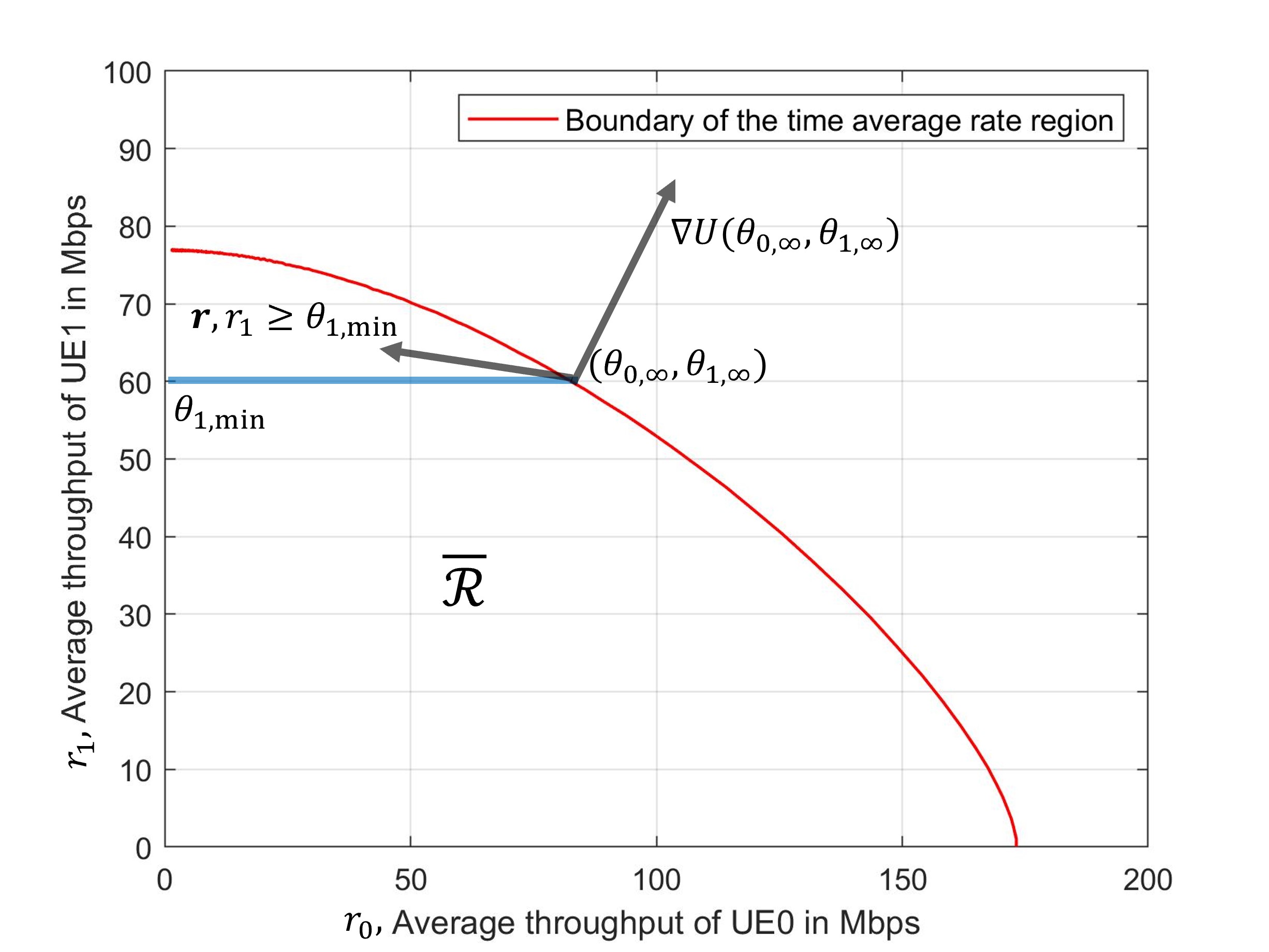
It follows that, for with , since , we have shown that (see Figure 1 for an illustration)
| (17) | |||||
Since is a closed convex set, and is strictly concave, it follows from [5, Chapter 3, Page 103] that is the unique utility maximising throughput vector with a rate guarantee for .
The above argument suggests that the sequence of EWMA throughputs will, in large time, become close to . This is formalized in the next section.
IV-B Main result on convergence with rate guarantees
In this section, under certain conditions, we analyze the algorithm defined by Equations (4)-(6) using the approach for weak convergence of two-time-scale constant step-size stochastic approximation provided in [8, Section 8.6]. We culminate this section in Theorem 1 which is the main convergence result for the Lagrange multipliers.
Define the sequence of -fields, , as follows:
Further, define:
| (18) | |||||
and observe that does not depend on or on . The so-called martingale difference “noise” in the rate recursion (5) is defined by:
| (19) | |||||
For the index-bias recursion (6), we define
| (20) |
with the associated martingale difference noise being zero. With these definitions, we rewrite Equations (5)-(6) as follows:
| (21) | |||||
| (22) |
The result we will apply is [8, Theorem 8.6.1]. To apply this result, we proceed to verify that the conditions A8.6.0 to A8.6.5 (in [8, Section 8.6.1]) hold in our problem.
A8.6.0 The projection applied to the index-bias is on a hyperrectangle, of the type described in [8, A 4.3.1]).
A8.6.1 We notice that are compact sets, and for each . Further, by rewriting Equation (5) as follows,
| (23) | |||||
we observe that will always be in a compact set, and uniform integrability of the family of random vectors , where the random vectors are indexed by and , holds. It follows that
is uniformly integrable, and moreover, for each fixed and ,
is also uniformly integrable.
We further require that the sequence of random variables is tight. Condition 1 below implies this.
Condition 1
Assume that the channel state process belongs to a compact set in .
A8.6.2 We need the continuity of uniformly over and . Here, the do not matter; we need the continuity of over uniformly in .
Following [2], we require:
Condition 2 (Strict Convexity of Rate Regions)
Assume that for every , and , is unique, and, also, is unique.
The strict convexity is understood to apply to the Pareto optimal boundary of the rate regions.
Further, we require:
Condition 3
Assume that for , the mappings and are continuous.
If the is polyhedral for each , Condition 3 may hold if is a continuum222In the sequel, we will continue to use the notation and with the understanding that these should be intrepreted as integrals and transition kernel densities, respectively, when is a continuum., for example when we are dealing with Rayleigh fading with truncation to a compact set (in view of Condition 1).
Analogous to (14), using Condition 2, it is easily seen that (see [2]):
| (24) |
Since is continuous in , Condition 3 and the compactness of implies that is continuous over uniformly in .
Trivially, is continuous in .
A8.6.3 Fix . Consider the following (notice that the step sizes do not play any role) for a suitable continuous function :
in probability, where we have used ergodicity of the Markov chain of channel states and the uniform integrability of in the last equality and refers to the expectation with respect to the stationary distribution of the Markov chain. It follows that, for the last term in the above sequence of equalities to be equal to ,
| (25) | |||||
is the desired function. The second equality requires Condition 2, and the continuity of with respect to follows from Condition 3.
A8.6.4 We now need to show that, for fixed , the o.d.e.
| (26) |
has a unique globally asymptotically stable point that is continuous in , characterized by
| (27) |
We first argue that the rest point of the dynamics (26) is unique for each , and that the rest point is . Consider the optimization problem . This is the maximization of a strictly concave function over a convex set; hence, the solution, say , is unique. Further, this optimum solution must satisfy for all ; i.e., . Observe from (27) that this , so the right-hand-side of (25) is zero at , and hence is the unique rest point for the o.d.e. (26).
In the Appendix, we show that is globally asymptotically stable for the o.d.e. (26).
Continuity of the unique stable point with : Continuing the previous argument, we have . Consider the sequence, indexed by , in . For every , , a compact set. Thus, consider a subsequence and . Since is continuously differentiable, . Hence, by Condition 2,
i.e., , or . By the uniqueness, proved above, . This holds for every convergent subsequence of . Hence, , and we conclude that is continuous in .
A8.6.5 We first need to show uniform integrability of the sequence , and, for each , of the sequence . The first follows because the sequence belong to a compact set. The second is trivial because is independent of .
Further, we must show that there is a continuous function such that for each , in probability, the following holds:
i.e.,
It follows that the desired function is
| (28) |
which is continuous in by A8.6.4.
The following condition on the optimization problem in Equation (1) ensures that we can restrict to a compact set:
Condition 4
There is a such that the optimum Lagrange multipliers (dual variables) of the optimization problem (1) lie in the set .
In the Appendix, we illustrate how this condition can be checked, by providing an example of a two UE problem.
With all the above conditions having been met, along with the o.d.e. in Equation (26), [8, Theorem 8.6.1] considers the following o.d.e. for the index-bias.
| (29) |
where is the term that compensates for the dynamics so that stays in its constraint set; here is the cone of outward normals to the constraint set at .
Let denote the set of limit points of the dynamics (29) in over all initial conditions. For a , let denote the -neighborhood of . Define the continuous time interpolation for as:
The foregoing has established the following theorem.
Theorem 1
Proof:
All assumptions A8.6.0 to A.8.6.5, in order to apply [8, Theorem 8.6.1], have been verified above, and the theorem follows. ∎
IV-C Stable rest points and the optimum solution
We now use properties of the joint stable points of the o.d.e. in Equation (26) and the o.d.e. in Equation (29), i.e., , to show that these correspond to the optimal solution of the optimization problem in Equation (1).
Consider a stable rest point of the o.d.e. in Equation (29). Such a rest point is in . Using Equation (27), we can write, for every :
Transposing, we obtain, for every :
| (31) | |||||
Since is stable rest point for the o.d.e. in Equation (29), and , it follows that, for (the number of UEs):
Note that the case cannot be a stable rest point of the o.d.e. Equation (29).
Returning to Equation (31), and utilising Equations (IV-C), we conclude that for ,
From [5, Chapter 3, Page 103], we see that are optimal for the optimization problem in Equation (1). Since the optimization is one of a strictly concave function over a convex set, the solution is unique, and is the correct set of Lagrange multipliers.
Thus is a joint unique stable rest point for the joint o.d.e. system in Equation (26), with replaced by , and Equation (29).
We have already seen, in the verification of A8.6.4, that, for fixed index-bias , the EWMA rate recursion yields the o.d.e. in Equation (26) which has the unique globally asymptotically stable point , characterized in Equation (27), and continuous in . Further, the index-bias recursion yields the o.d.e. in Equation (29). Theorem 1 establishes that if, in addition, , then, for large , are close to , which solve the optimization problem in Equation (1). In other words, the throughput iterates converge to the optimum solution. A note of caution however is that could contain limit cycles for the dynamics in (29). In the simulation experiments, we see that we do not have such issues on the examples considered.
V Simulation Experiments
We will carry out simulation experiments for the utility function , which satisfies all the mathematical properties in our earlier development. With a slight abuse of terminology, we will call the resulting rate allocation proportionally fair, even though the addition of a 1 to the rate is a deviation from the commonly accepted . For modern wireless networks, the rates available to UEs are very high (several 10s of Mbps); the addition of the 1 will not result in a significant difference in the final rate allocation, and reduces mathematical complexities. The rate allocation algorithm with rate guarantees, presented in Section III-B will be referred to as PF-RG-LM (Proportional Fair scheduling with Rate Guarantees, using the Lagrange Multiplier approach).
V-A The PF-RG-TC algorithm
In [9, 3], Mandelli et al. have also provided an index-bias based algorithm. They maintain a token counter (denoted, here, by ) which is used to bias the rate allocation index. We call their algorithm PF-RG-TC (for Token Counter). Following the notation in Equations (4), (5), and (6), we write the PF-RG-TC as follows.
There is a single small step-size . At the beginning of slot , given the joint channel state , the EWMA throughputs , and the token counters , determine as follows (see [9, Equations (4) and (5)]):
| (33) | |||||
The EWMA throughputs are updated as follows.
| (34) | |||||
For all , the index biases are updated as follows.
| (35) | |||||
V-B Wireless communication model
All our simulations are for the following generic wireless communication setting. The channel is in the 2.4 GHz band, and the system bandwidth is MHz. The noise floor is taken as dBm; there are no interferers. For the BS transmit power dBm, the mean received power at distance m is given by , where is the attenuation at m, and the pathloss exponent is . Rayleigh fading is assumed, which results in exponentially distributed attuation in dB, with parameter 1. The slot duration is sec.
In slot , the received signal strengths are sampled as above. Then, the rates available to the two UEs are obtained independently (in time and across the UEs) from the Shannon channel capacity formula as follows:
V-C Two UEs: Rate regions
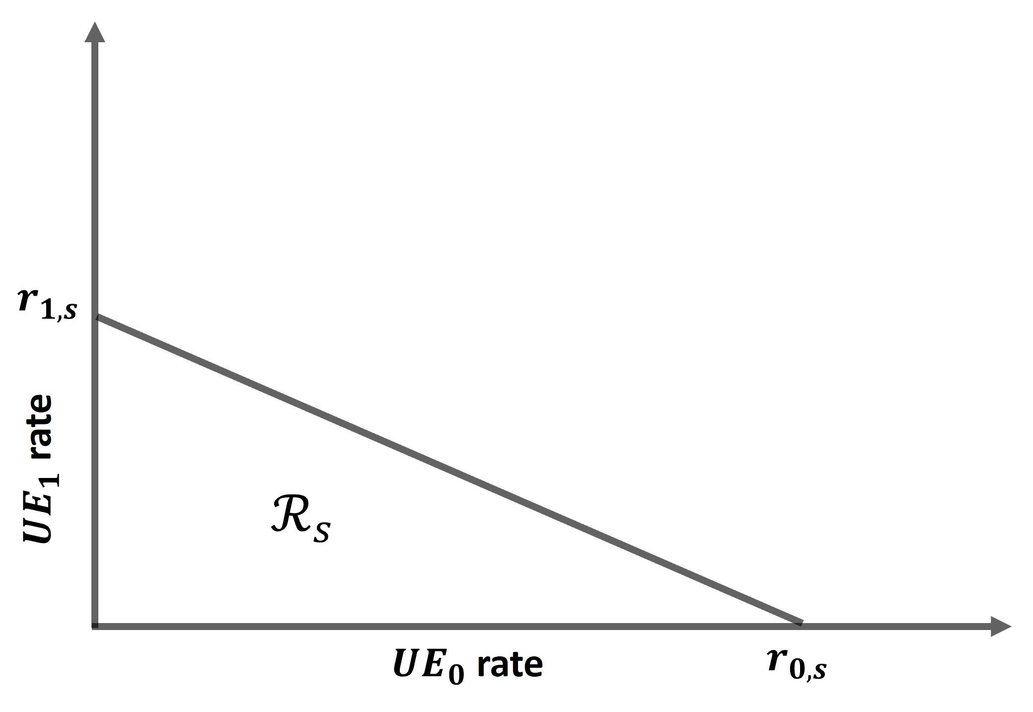
There are two UEs, and , at the distances of m and m from the gNB. With the wireless channel model in Section V-B, and dBm, the rate region in a slot, , has the triangular shape depicted in the left panel Figure 2. For such a rate region for two UEs, when the calculation in Equation (4) is done, it is of the form for some . Due to the shape of , this will result in one of the two UEs being scheduled in each slot.
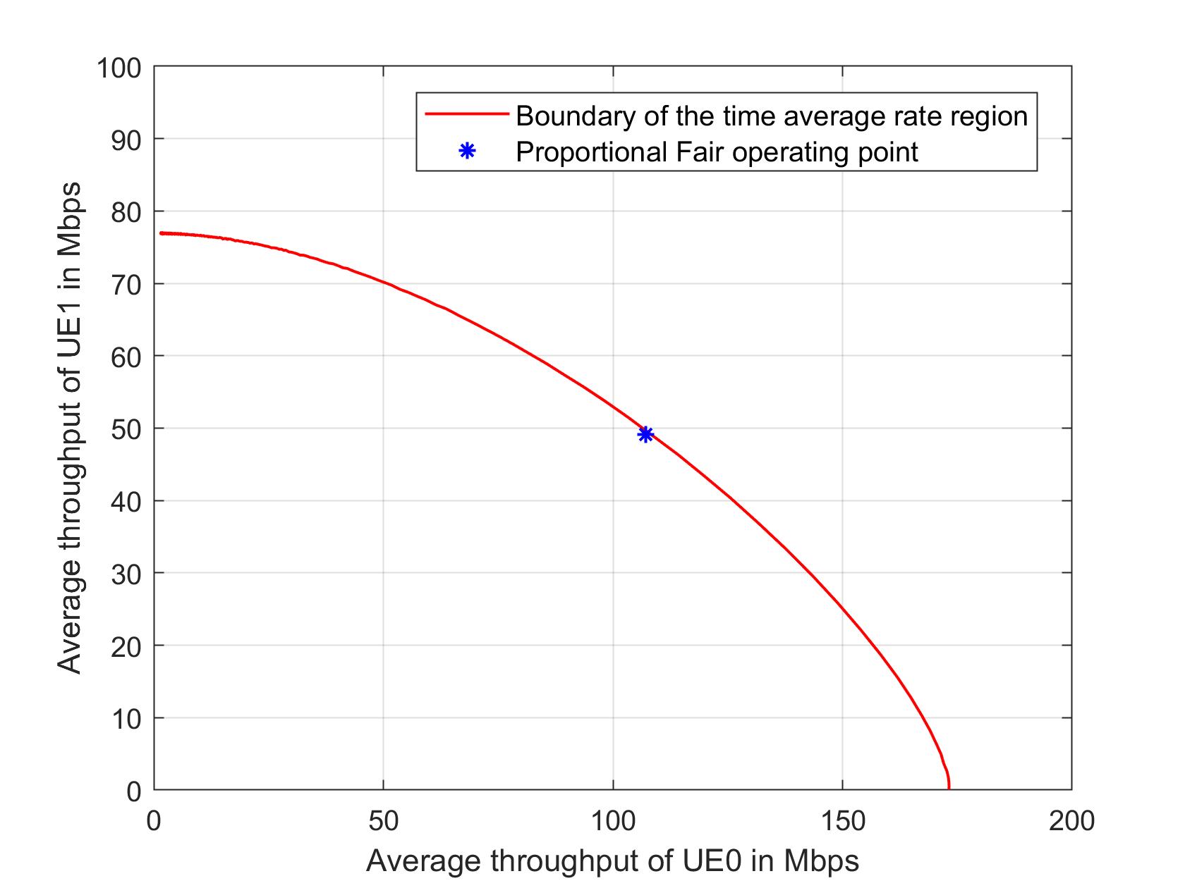
The rate region, time averaged over all channel states, , is shown in the right panel of Figure 2, along with the proportional fair operating point (for the utility ). The outer boundary of has been obtained by simulating the above wireless channel model for slots, and obtaining the operating points for the utility for a range of values of .
V-D Two UEs: Index-bias smoothing, & slow time scale updates


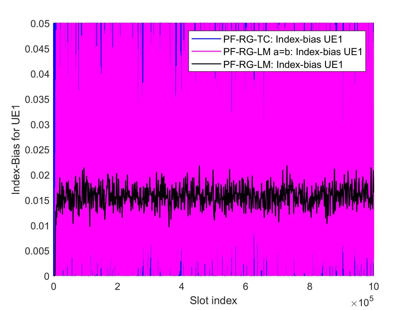

In Figures 3, 4, and 5 we show the results from running the PF-RG-LM (with , and ), and PF-RG-TC algorithms on rate data generated by the wireless communication model described in Section V-B, with the BS transmit power set at mW. With (left plots) all three approaches provide an average rate of about Mbps to , but PF-RG-TC and PF-RG-LM (with ) provide lower rates to . Figure 5 shows that the index-bias for PF-RG-TC fluctuates wildly, not appearing to follow any trend; with , PF-RG-LM provides a slightly more controlled but still highly fluctuating index-bias. With the index-bias being updated at a much slower time-scale than the EWMA rates, the index-bias for PF-RG-LM fluctuates slowly around a steady-state value. With (right plots) the throughputs provided by PF-RG-TC are far from optimum. PF-RG-LM with and both provide accurate tracking of the optimum operating point. The index-bias for PF-RG-LM with is better controlled but still fluctuates significantly. On the other hand with a slower time-scale update, PF-RG-LM not only provides an accurate tracking of the optimum EWMA throughputs, but hovers around a value of approximately .
We may infer that the two-time scale stochastic approximation algorithm used in PF-RG-LM provides not only an accurate throughput operating point with rate guarantees, but also an accurate tracking of the Lagrange multipliers. We notice, from Equation (35), that in PF-RG-TC, in addition to stochastic approximation not being used in the token counter update, the token counter is updated by the rate allocation in the previous slot, rather than the EWMA rate, as in PF-RG-LM (see Equation (6)).
V-E PF-RG-LM with UEs
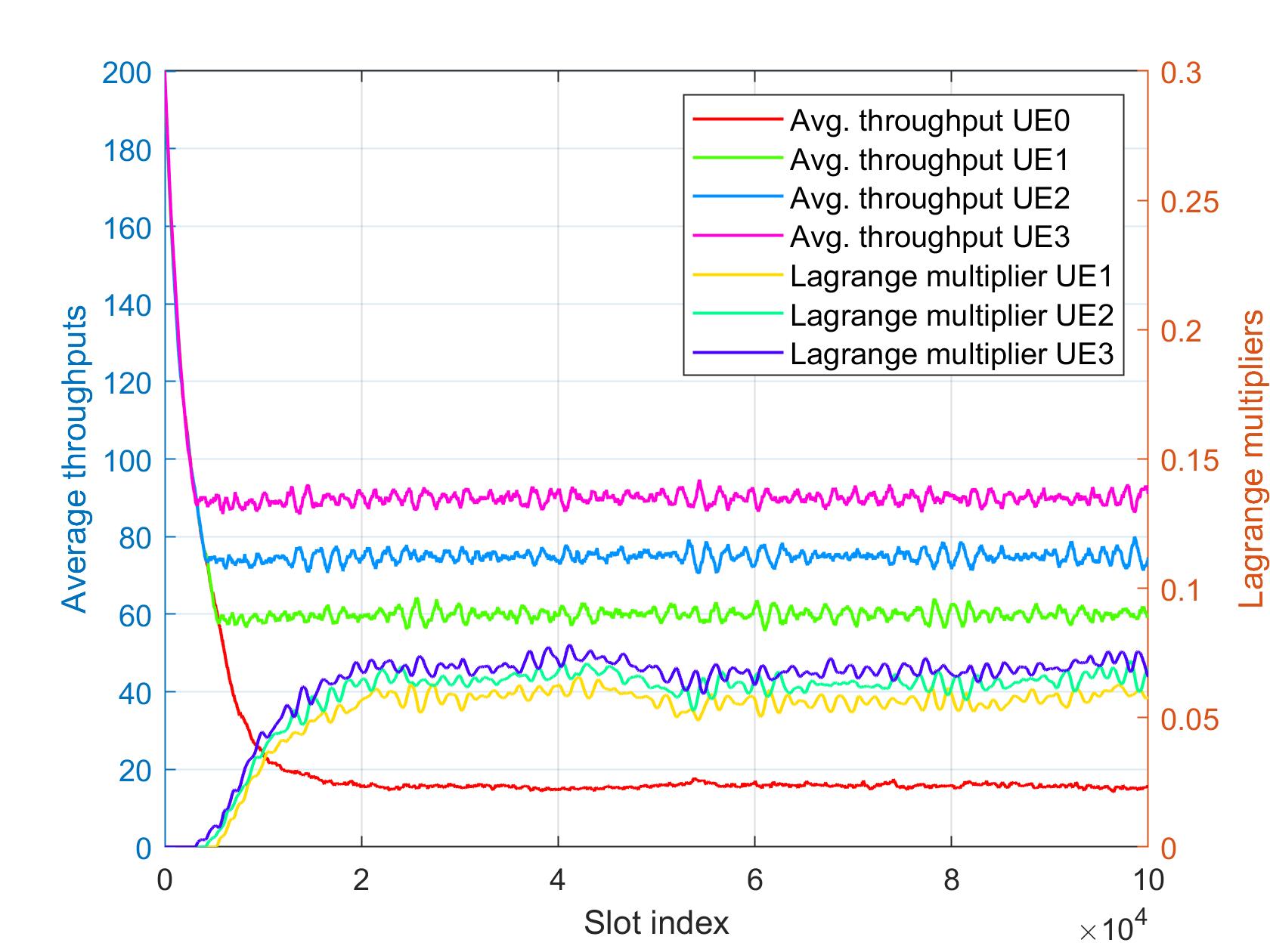
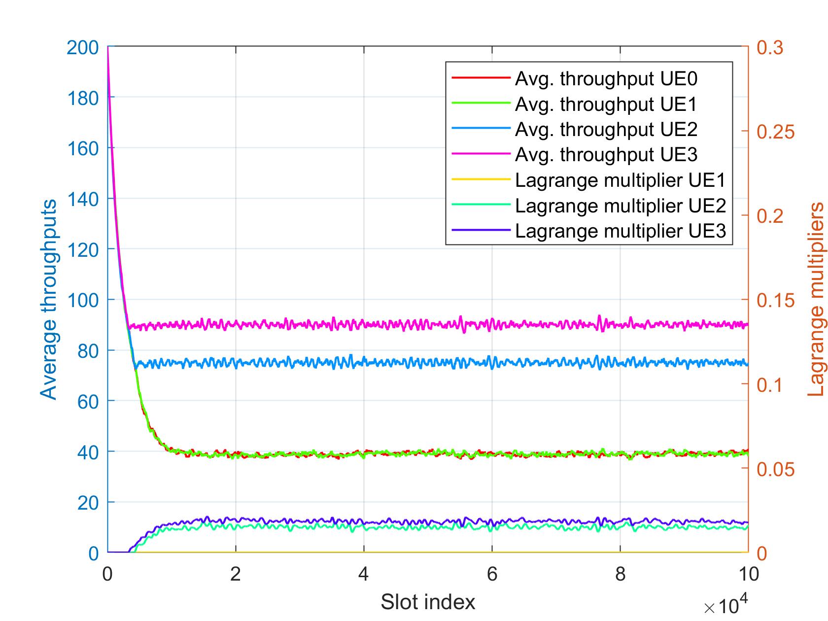
In Figure 6, we provide results from running PF-RG-LM on rate data generated from the wireless communication model described in Section V-B, with 4 UEs, all at m from the BS, and the BS transmit power set at mW. In the left plot, the rate guarantees are Mbps for , , , and , and in the right plot these are . Both plots show that the UEs with rate guarantees obtain their respective guaranteed rates. In the left plot, achieves a rate of a little over Mbps, whereas for the case in the right plot, and achieve the same rate of about Mbps. The Lagrange multipliers also stabilize, with the larger guaranteed rate corresponding to the larger Lagrange multipliers, as expected. Notice that, in the right plot for all .
V-F Polyhedral average rate region,
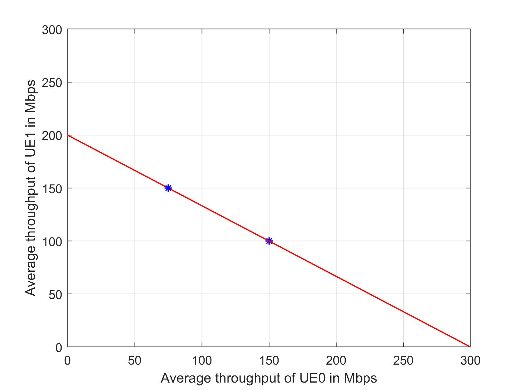
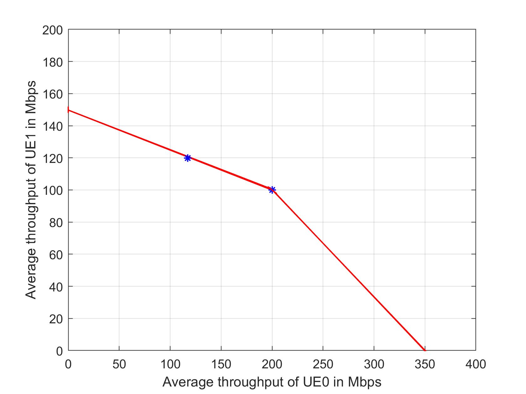
Figure 7 shows that the algorithms with and without rate guarantees work correctly even when the rate region, , is not strictly convex. In the left plot, the channel has one state, i.e., , and, in each slot one of the UEs will be scheduled. However, time-sharing occurs over time, yielding the desired throughputs. In the right plot, the channel has two states, i.e., ; has the ployhedral shape shown. While the PF-RG-LM algorithm works correctly, our convergence proof does not apply to this case. This remains an item of our current work.
VI Conclusion
Assuming feasibility of the utility optimization problem, we have proposed a slow time-scale update for the additive index-bias that promotes rate guarantees in the usual gradient-type scheduling algorithm. We provide a convergence proof of this algorithm for strictly convex average rate regions. Our simulations show that the slower time-scale index-bias update not only provides accurate maximum utility throughputs, but the index-biases provide very good approximations to the optimum Langrange multipliers. Practical considerations might require that the throughput averaging time-scale might be specified by the standard or by user requirements, in which case, having a separate time-scale for the index-bias update would be useful for providing a very good estimate of the optimum Lagrange multiplier.
Appendix
Global asymptotic stability
We now argue that, for a fixed , the o.d.e. (26) has a unique globally asymptotically stable equilibrium. The following proof has been taken from [11], and is provided here for completeness. Recall that (26) is
Let denote the distance of to the set . We first argue that .
Let denote the projection of on . Let
Observe that and are continuous in , the latter following from Condition 3. For , , and hence can be used to bound the distance to at time for sufficiently small. We can then upper bound the rate of change of the distance of to the set as follows:
where the penultimate equality requires an argument that uses the continuity of and in .
Thus, for any and any bounded set on the positive orthant, there exists a such that for all , where is the -thickening of , which is the set of all points that are within a distance of .
We recall Equation 27, which defines as the maximizer of in . Now, fix an arbitrary , and denote by the open ball of radius around the maximizer. Fix small enough so that the maximum of in , denoted , satisfies
Given that , a compact set, the dynamics enters and remains there for all . Further, given that so long as the dynamics remains in , we have
where the second inequality follows from concavity of in . This implies that the dynamics must exit at some time . Combining this with the fact that the dynamics remains in for all , we conclude that for all . Since was arbitrary, we conclude that , which establishes the desired global asymptotic stability.
Obtaining : Two UE Example
To illustrate how it can be determined if there is a bound on the optimum Lagrange multipliers, we provide an illustration for two UEs, and in which has the minimum rate guarantee . By sensitivity analysis of the optimum solution of the optimization problem (1), we can conclude that:
where is the optimum primal solution, and the optimal dual solution. It follows that
Where, in the second term, we have assumed that is strictly feasible, i.e., the rate guarantee can be increased. At the point on the boundary of the average rate region let be the normal to the boundary. It follows that , which yields
One way to satisfy Condition 4 is to ensure that the right hand side of the above inequality is bounded.
References
- [1] 3GPP. System Architecture for the 5G System (3GPP TS 23.501 version 15.2.0 Release 15), 2018.
- [2] R. Agarwal and V. Subramanian. Optimality of certain channel aware scheduling policies. In Proc. 40th Annual Allerton Conference on Communications, Control, and Computing, 2002.
- [3] M. Andrews, S. Mandelli, and S. Borst. Network slicing based on one or more token counters. United States Patent, February 2021. Patent Number US 2021/0037544 A1.
- [4] Albert Banchs, Gustavo de Veciana, Vincenzo Sciancalepore, and Xavier Costa-Perez. Resource allocation for network slicing in mobile networks. IEEE Access, 8, 2020.
- [5] M. S. Bazaara, H. D. Sherali, and C. M. Shetty. Nonlinear Programming: Theory and Algorithms. John Wiley and Sons, Inc., 1993.
- [6] V. S. Borkar. Stochastic Approximation: A Dynamical Systems Viewpoint. Hindustan Book Agency, 2008.
- [7] H. J. Kushner and P. A. Whiting. Convergence of proportional-fair sharing algorithms under general conditions. IEEE Transactions on Communications, 3(4), 2004.
- [8] Harold J. Kushner and G. George Yin. Stochastic Approximation Algorithms and Applications. Springer, 2003.
- [9] S. Mandelli, M. Andrews, S. Borst, and S. Klein. Satisfying network slicing constraints via 5G MAC scheduling. In Prof. IEEE Infocom 2019, April 2019.
- [10] Ravi Kiran Raman and Krishna Jagannathan. Downlink resource allocation under time-varying interference: Fairness and throughput optimality. IEEE Transactions on Wireless Communications, 17(2), 2018.
- [11] A. L. Stolyar. On the asymptotic optimality of the gradient scheduling algorithm for multiuser throughput allocation. Operations Research, 53(1):12–25, 2005.
- [12] Alexander L. Stolyar. Greedy primal-dual algorithm for dynamic resource allocation in complex networks. Queueing Systems, 54, 2006.