Point Source Identification Using Singularity Enriched Neural Networks††thanks: The work of B. Jin is supported by Hong Kong RGC General Research Fund (Project 14306423), and a start-up fund and Direct Grant for Research, both from The Chinese University of Hong Kong. The work of Z. Zhou is supported by Hong Kong Research Grants Council (15303122) and an internal grant of Hong Kong Polytechnic University (Project ID: P0038888, Work Programme: 1-ZVX3).
Abstract
The inverse problem of recovering point sources represents an important class of applied inverse problems. However, there is still a lack of neural network-based methods for point source identification, mainly due to the inherent solution singularity. In this work, we develop a novel algorithm to identify point sources, utilizing a neural network combined with a singularity enrichment technique. We employ the fundamental solution and neural networks to represent the singular and regular parts, respectively, and then minimize an empirical loss involving the intensities and locations of the unknown point sources, as well as the parameters of the neural network. Moreover, by combining the conditional stability argument of the inverse problem with the generalization error of the empirical loss, we conduct a rigorous error analysis of the algorithm. We demonstrate the effectiveness of the method with several challenging experiments.
Key words: point source identification, neural network, singularity enrichment, error estimate
1 Introduction
Inverse source problems (ISP) represent an important class of applied inverse problems, and play an important role in science, engineering and medicine. One model setting is as follows. Let be an open bounded domain with a smooth boundary . Let denote the unit outward normal vector to , and denote taking the outward normal derivative. Consider the standard Poisson equation
| (1.1) |
The concerned inverse problem is to determine the source from the Cauchy data . In practice, we can only access noisy data with a noise level , i.e. and .
The ISP for the Poisson equation has been extensive studied (see the monographs [1, 27]). With only one Cauchy data pair, it is impossible to uniquely recover a general source : Indeed, adding any smooth function with a compact support to does not change the Cauchy data. Thus, suitable prior knowledge (i.e., physical nature) on the source is required in order to restore unique identifiability. It is known that one Cauchy data pair can uniquely determine the unknown source , e.g., one factor of a product source (i.e. is separable and one factor is known) [32, 15], or the angular factor of a spherically layered source [15], or or (with being the characteristic function of a polygon , and a nonzero constant vector) [26].
In this work, we investigate the case that is a linear combination of point sources:
| (1.2) |
where is the Dirac delta function concentrated at , defined by for all , and is the intensity of the point source at the point . The unknown parameters include the number of point sources, and the locations and intensities . It arises in several practical applications, e.g., in electroencephalography, the Dirac function can describe active sources in the brain [37, 36]. The specific inverse problem satisfies unique identifiability, and Hölder stability [13, 14].
Numerically, El Badia et al [16] developed a direct method to identify the number and locations / intensities for the Poisson problem in 2D domains. From the Cauchy data , we can compute the value for any harmonic . By suitably choosing , we can determine the number , and locations and densities of the point sources. It works well for both 2D and 3D cases, for which is constructed from complex analytic functions. It is more involved in the high-dimensional case [9]: both constructing the harmonic test function and computing the reciprocity gap functional (cf. (2.1)) are nontrivial. We aim at developing a novel neural method for the task using neural networks (NNs). The key challenge lies in the low regularity of point sources, and the low regularity of the associated PDE solution. Thus, standard neural solvers are ineffective in resolving the solution . To overcome the challenge, we draw on the analytic insight that can be split into a singular part (represented by fundamental solutions), and a regular part that can be effectively approximated by NNs.
In this work, we develop a novel numerical method for recovering point sources using NNs. The proposed method consists of two steps. First we detect the number of point sources as [16], and then learn simultaneously the smooth part (approximated using NNs) and parameters of the unknown point sources (i.e., the intensities and locations) using a least-squares type empirical loss. In sum, we make the following contributions. First, we develop an easy-to-implement algorithm for recovering point sources. Second, we provide error bounds for the algorithm. This is achieved by suitably combining conditional stability with a priori estimates on the empirical loss, using techniques from statistical learning theory [2]. We bound the Hausdorff distance between the approximate and exact locations, and errors of the intensities and the regular part, explicitly in terms of the noise level, neural network architecture and the numbers of sampling points in the domain and on the boundary. Third, we present several numerical experiments, including partial Cauchy data and Helmholtz problem, to illustrate its flexibility and accuracy.
Now let us put the work into the context of neural solvers for ISPs. Solving PDE inverse problems using neural networks has received much recent attention in either supervised or unsupervised manners. Nonetheless, neural solvers for ISPs are still very limited. Zhang and Liu [43] employed the deep Galerkin method [40] to recover the source term in an elliptic problem using the measurement of the solution in a subdomain, and established the convergence of the method for analytic sources; see also [44] for the parabolic case. Li et al [33] investigated the use of DNNs for the stochastic inverse source problem. In contrast, this work focuses on identifying point sources which is strongly nonlinear but enjoys Hölder stability, which enables deriving a priori error estimates for the proposed neural solver. Du et al [12] developed a novel divide-and-conquer algorithm for recovering point sources for the Helmholtz equation. In contrast, this work contributes one novel unsupervised neural solver for identifying point sources and provides rigorous mathematical guarantee.
The rest of the paper is organized as follows. We develop the method in Section 2. In Section 3, we provide an analysis of the method. In Section 4, we present numerical experiments to illustrate the performance of the method, and give concluding remarks in Section 5. In the appendices, we collect several technical estimates for analyzing the empirical loss. Throughout, we use the notation to denote a constant which depends on its argument and whose value may differ at different occurrences.
2 The proposed method
Now we describe the proposed method, termed as singularity enriched neural network (SENN), for identifying point sources. The procedure consists of two steps: (i) detect the number of point sources and (ii) estimate the locations and intensities with singularity enrichment. Throughout, for a harmonic function , we denote by the following functional
| (2.1) |
and often abbreviate it to . It is commonly known as the reciprocity gap functional. It will play a key role in establishing the stability estimate.
2.1 Detection of the number of sources
First we recall the detection of the number of point sources. We only describe the case , following [16]. Note that the real or imaginary part of a complex polynomial is harmonic. By setting , we obtain
Given an upper bound , we can find using the next result [16, Lemma 2]:
Proposition 2.1.
Let the Hankel matrix , with . Then and the first columns of are linearly independent.
Proposition 2.1 suggests that we may start with the first column of , work forward one column each time, and stop the process when the columns become linearly dependent. The stopping index gives . In practice, due to the presence of quadrature error in evaluating the entries , one should enforce the stopping criterion inexactly. Let be the -th column of , , and let be the smallest singular value of . If , a given tolerance, then we claim that the columns are linearly dependent. The whole procedure is shown in Algorithm 1.
For the stability of the method, we define the Vandermonde matrix by
and let . The -th column of is , and . Let . Then we have Since is a submatrix of , we have , which is independent of . Thus, in theory, we may pick the tolerance in Algorithm 1, and in practice, fix it at about the noise level (including quadrature error etc).
2.2 Singularity enrichment
Once the number is estimated, we apply deep learning to learn the solution and the locations and densities. Due to the presence of point sources, is nonsmooth, and standard neural PDE solvers are ineffective [24]. We employ singularity enrichment, which splits out the singular part, in order to resolve the challenge. This idea has been widely used in the context of FEM [18, 7, 8, 19], and also neural PDE solvers [24, 25]. We extend the idea to recover point sources.
We employ the fundamental solution to the Laplace equation [17, p. 22]:
| (2.2) |
with and for , with . By definition, for any , satisfies in . We abbreviate as . Using , we can split the solution to (1.1) as
| (2.3) |
The term captures the leading singularity of the solution due to the point sources and is the regular part. The regular part satisfies
| (2.4) |
In (2.3), we have used the information about the unknown point source. This reformulation motivates the following loss for noisy data:
where is the weight vector, the vector of intensities, and the matrix of locations. We denote the loss for the exact data by , and its minimizer by . Note that .
2.3 Reconstruction via SENN
To approximate the regular part , we employ standard fully connected feedforward NNs. These are functions , with the parameter . It is defined recursively by , , , and , where , , with and . is a nonlinear function, applied componentwise to a vector, and we employ the hyperbolic tangent . The integers and are the depth and width. The parameters and are trainable and collected in a vector . We denote by the set of NN functions of depth , with the total number of nonzero parameters , and each entry bounded by , using the activation function :
| (2.5) |
where and denote the number of nonzero entries in and the maximum norm of a vector, respectively. Below we also use the shorthand notation .
We employ an element to approximate the regular part , and discretize relevant integrals using quadrature, e.g., Monte Carlo. Let be the uniform distribution over a set , and let denote its Lebesgue measure. Then we can rewrite the loss as
where denotes taking expectation with respect to . Let and be identically and independently distributed (i.i.d.) sampling points drawn from and , respectively, i.e., and . Then the empirical loss is given by
| (2.6) |
The resulting training problem reads
| (2.7) |
with being the NN approximation. Since is finite-dimensional and lives on a compact set (due to the bound ), and we further assume , for smooth , the loss is continuous in , which directly implies the existence of a global minimizer. Problem (2.7) is nonconvex, due to the nonlinearity of the NN in . Hence, it may be challenging to find a global minimizer of . In practice, gradient type algorithms, e.g., Adam [31] or L-BFGS [6], seem to work fairly well [30]. The gradient of with respect to the NN parameters and the NN with respect to the input can be computed via automatic differentiation. Thus, the method is easy to implement.
3 Error analysis
Now we give an error analysis of the method in Section 2 in order to provide theoretical guarantee. The analysis is challenging due to the nonlinearity of the ISP. Our analysis combines conditional stability of the ISP with the consistency error analysis for the empirical loss. For neural solvers for PDE direct problems, the analysis of the empirical loss has been studied (see, e.g., [28, 34, 24]).
3.1 Conditional stability
First we analyze the stability of the loss . Throughout, let and be the Euclidean distance between and . Let be the minimal distance of the set of points to , and let
| (3.1) |
Then . Let , with being the diameter of . Further, we assume that , . Let be a minimizer of over the set with .
First we bound the error of the empirical risk minimizer relative to the exact one using the population loss value . The proof is inspired by the conditional stability analysis of the ISP in [13, 14]. The key is to multiply with equation (1.1) some carefully constructed test functions and to exploit the reciprocity gap functional . Then using analytical properties of Vandemonde type matrices, we can obtain conditional stability for identifying point sources from Cauchy data. The construction relies on the harmonicity of complex analytic functions, which exist only in the two-dimensional complex plane, and we project the points in the general -dimensional domain into two-dimensional complex plane. More specifically, for one configuration , with , we denote by , , to be its projection onto -complex plane and let . Then we define the separability coefficient of the projected sources and the distance by
| (3.2) |
For two point configurations and , we make the following separability assumption for the subsequent analysis.
Assumption 3.1.
There exists a such that .
We define the Hausdorff distance by
We have the following stability result in Hausdorff distance.
Theorem 3.1.
Let and be minimizers of the losses and , respectively. Then under Assumption 3.1, there holds
Proof.
Let . Then and satisfy
| (3.3) |
respectively, with and given by
| (3.4) |
Now consider the -dimensional complex harmonic functions:
| (3.5) |
Setting in the reciprocity gap functional (cf. (2.1)) gives
Next multiplying with and then integrating by parts twice yield
Subtracting the preceding two identities yields that for ,
which, upon substituting the definition of , is equivalent to
Using the separability coefficient defined in (3.2) and Assumption 3.1, we have
Meanwhile, by the Cauchy-Schwarz inequality, we have
By the definition of , we have on , and then
Likewise, , on , and hence, Thus, we have
Then, taking the maximum over and using the definition of lead to
| (3.6) | ||||
Similarly, with , we have
| (3.7) | ||||
Now using the definition of Hausdorff distance gives
| (3.8) |
Further, direct computation yields
That is, . The assertion follows from (3.8). ∎
By Theorem 3.1 and the Hall-Rado theorem in graph theory, we have the following error bound when . The condition will be assume below.
Theorem 3.2.
Let Assumption 3.1 be fulfilled. For two point configurations and , if , there exists a permutation of the set such that
| (3.9) |
Theorem 3.3 (Hall-Rado [39]).
Consider an even graph having nodes and , and connect some pairs such that for every and every subsequence of , at least elements of the sequence are connected to one of them. Then there exists a permutation of the integers such that is connected to for every .
Proof of Theorem 3.2.
The result is direct from Theorem 3.1; see the proof of [14, Theorem 3.2]. We recap the proof for completeness. We connect the even graph in the way that is connected to if for . We claim that for every and every subsequence of , at least elements of are connected to one of them. Otherwise, there exists one subsequence of and at least one in , there holds for all , which leads to a contradiction with the definition of Hausdorff distance. Then the desired result follows directly from the Hall–Rado theorem. ∎
Next we bound the error of the recovered densities .
Theorem 3.4.
Proof.
Fix , and let be the projection of onto the -complex plane. For , define the harmonic functions
Testing (3.3) with and using in (2.1), with and defined in (3.4), yield
| (3.11) | ||||
| (3.12) |
Next we define two Vandermonde matrices
and four vectors in , i.e.,
Then we can rewrite (3.11) and (3.12) into and . Taking their difference yields
and consequently,
| (3.13) |
Meanwhile, [20, Theorem 1] gives
| (3.14) |
Since , we have , and , and . This leads to
| (3.15) |
Likewise, we have
Combining the preceding estimates yields with ,
This estimate and Theorem 3.2 imply the desired result. ∎
Next we analyze the error of the regular part in terms of the population loss.
Proof.
Let be the permutation given in Theorem 3.2, let , and let
| (3.17) |
Then with and in (3.4), we have
| (3.18) |
Now we define the harmonic extension of by
The following elliptic regularity estimate holds [4, Theorem 4.2, p. 870]
| (3.19) |
Let . Then it satisfies
Since , the Poincaré inequality and the standard energy argument imply
This, the triangle inequality, and the stability estimate (3.19) lead to
This estimate, the triangle inequality and the identity (3.18) imply
| (3.20) |
Meanwhile, by the definition of in (2.2),
with . Next we bound and . From the splitting (3.17) and by combining the preceding estimates with Theorems 3.2 and 3.4, we obtain
Then substituting these two estimates into (3.20) yields the desired result. ∎
Finally, we gives an error bound on the approximation of the solution .
Corollary 3.1.
Let , and be the solution of (1.1). Then for any , there holds with ,
3.2 Generalization error analysis of the empirical loss
The analysis in Section 3.1 focuses on the population loss, evaluated at the minimizer of the empirical loss . In practice, we only minimize the empirical loss , and do not have access to the population loss . The analysis of the error between the empirical and population losses is commonly known as generalization error analysis in statistical learning theory [2], which is the main goal of this part. First we establish an important error splitting, which involves three components: the approximation error , the statistical error and the noise level . The first two components will be analyzed below.
Lemma 3.1.
Let minimize the loss (2.6) over the set . Then we have
Proof.
Let . By the triangle inequality, for any , we have
Similarly, we have These inequalities and the minimizing property of to the loss imply that for any ,
| (3.21) |
Using the facts and , and the trace theorem, we deduce
Combining this with (3.21) and taking the infimum over yield the result. ∎
Now we analyze the approximation and statistical errors separately. We make the following regularity assumption. Condition (i) and the standard elliptic regularity theory ensure that problem (2.4) admits a solution , which enables bounding the approximation error quantitatively. Condition (ii) is needed for bounding the Rademacher complexity of the function classes in Lemma A.4.
Assumption 3.2.
(i) and , and (ii) .
We employ the following approximation result [23, Proposition 4.8]. The notation equals to 1 if and zero otherwise.
Lemma 3.2.
Let and be fixed, and with . Then for any tolerance , there exists at least one of depth , with bounded by and bounded by , where is arbitrarily small, such that .
Under Assumption 3.2, the regular part belongs to . Thus, for any , by Lemma 3.2 with and , there exists
| (3.22) |
such that . Next, we bound the statistical error
which arises from approximating the integrals by Monte Carlo. Note that the discretization error is a random variable. In the statistical learning theory, such error is often bounded using Rademacher complexity. By the triangle inequality, we have
| (3.23) |
with for , and for . We define three function classes , and .
Using the technical estimates in Appendix A, we have the following bound on .
Theorem 3.6.
Proof.
Fix , , , and . By [10, Prop. 5], (cf. Def. A.2) is bounded by Lemmas A.3 and A.4 imply with ,
By Lemma A.4, we have . Then by setting in Lemma A.2 and using the facts , and , (for ), cf. Lemma 3.2, we can bound the Rademacher complexity by
We endow the space with , for any . Then is a metric and a metric space. Then using [10, Proposition 5] again we have
with . Similarly for the third term, there holds
with . Repeating the preceding argument yields
Finally, the desired result follows the PAC type bound in Lemma A.1. ∎
Last, we can state the main result of this part.
Theorem 3.7.
4 Numerical experiments and discussions
Now we present numerical examples to illustrate SENN. The gradient of with respect to the input (i.e., spatial derivative) and that of the loss with respect to are computed via automatic differentiation using torch.autograd. The empirical loss is minimized using Adam [31], as implemented in the SciPy library, with the default setting (tolerance =1.0e-8, no box constraint). The noisy data is generated as , for each sampling point , where follows an i.i.d. uniform distribution on , and the noisy Neumann data is generated similarly. The PyTorch source code for the numerical experiments will be made available at https://github.com/hhjc-web/point-source-identification.
The first example is the standard Poisson equation with point sources.
Example 4.1.
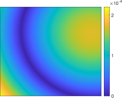
Let , and the harmonic function , with the information of the sources given in Table 1. Consider three cases: (i) full Cauchy data, (ii) Dirichlet data on the edges and Neumann data on , (iii) Cauchy data on .
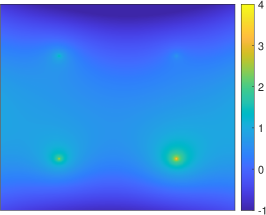
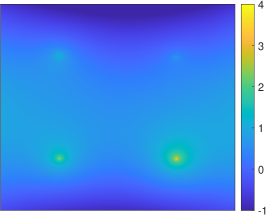
First, we employ Algorithm 1 to detect the number of point sources, with a tolerance (for the noise level ). The algorithm terminates at with the singular values (with 3 decimal places). We employ a 2-20-20-1 NN (2 hidden layers, each having 20 neurons) to approximate the smooth part , set the penalty weight , and take points in the domain and points on the boundary to form the empirical loss . Further, we set the learning rate to 1.0e-3 for NN parameters and 6.0e-3 for point densities and locations. The results for the densities and locations obtained after 10,000 iterations are shown in Table 1, which also includes the results by the algebraic method [16]. Both the proposed method and the algebraic method can give satisfactory results. The recovered in Fig. 1 shows that the pointwise error is small and the predicted locations of the point sources are quite accurate.
| point | density | location | density | location |
| exact | 1.000 | 2.000 | ||
| (i), SENN | 1.025 | 1.983 | ||
| (i), [16] | 0.977 | 2.047 | ||
| (ii) | 1.096 | 1.962 | ||
| (iii) | 1.026 | 1.975 | ||
| point | density | location | density | location |
| exact | 3.000 | 4.000 | ||
| (i), SENN | 3.022 | 3.973 | ||
| (i), [16] | 2.989 | 3.990 | ||
| (ii) | 3.038 | 3.899 | ||
| (iii) | 3.126 | 3.844 |
 |
 |
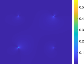 |
| (a) exact | (b) predicted | (c) error |
The smallest singular value of the Hankel matrix in Algorithm 1 increases with the noise level . If the noise level is very high, or the tolerance is not properly set, the number of point sources may be inaccurately estimated, which can affect the accuracy of the subsequent recovery. Nonetheless, Theorem 3.7 shows that the Hausdorff distance can still be properly bounded (under suitable conditions). Numerically, we test the noise level and choose different so that the number of point sources is incorrectly estimated to be 3 and 5 respectively, and then proceed to training. The estimated locations and densities of the point sources are shown in Table 2. The results indicate that for , the predicted point sources are still very satisfactory: it roughly amounts to splitting one or more sources, and their combined effect is close to the exact one. However, for , the predictions are not so satisfactory. Thus, when the noise level is high, one should set the tolerance slightly smaller, so that the number of predicted points is no less than the exact one . We repeat the experiment with the algebraic method [16]; see Table 3 for the results. It is observed that when the number of points is incorrectly estimated, the error is very large and the prediction is not reliable. This is attributed to the ill-conditioning of the Hankel matrix used in the algebraic method.
| exact | |||||
| density | location | density | location | density | location |
| exact | |||
| density | location | density | location |
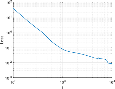
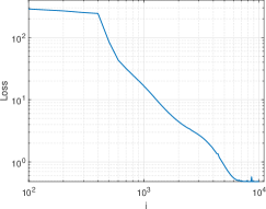
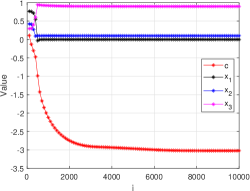
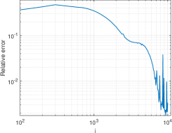
To shed further insights, we show in Fig. 2 the training dynamics of the empirical loss and the relative error (of the regular part ), where denotes the total iteration index. Both the loss and the relative error decay steadily as the iteration proceeds, indicating stable convergence of the Adam optimizer. However, as the number of iterations increases further, the loss trajectory exhibits oscillations while the error stays at a low level. This is typical for gradient type optimizers such as Adam [5]: Large learning rates or gradients can cause oscillations. The final error saturates at around , which agrees with the observation that the accuracy of neural PDE solvers tends to stagnate at a level of [41]. Fig. 3 shows the dynamics of the recovered density and location of each point source during the training, where is initialized randomly in the domain , and the density is initialized randomly in . Numerically, we observe that the densities takes longer time to reach convergence than the locations , but after 10,000 iterations both densities and locations stabilize at the minimizer.
 |
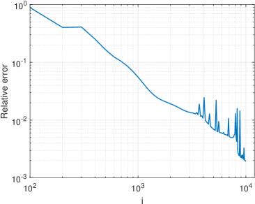 |
| (a) loss vs | (b) relative error vs |
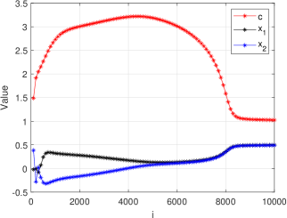 |
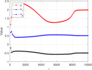 |
| (a) point 1 | (b) point 2 |
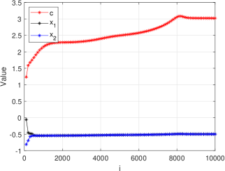 |
 |
| (c) point 3 | (d) point 4 |
In practice, we may only know partial Cauchy data, for which we illustrate two cases (ii) and (iii). Since the algebraic method does not work any more for partial data, we assume that the number of point sources is given. To form the empirical loss , for case (ii), we take observation points for Dirichlet data, for Neumann data, and in the domain , and for case (iii), we take the number of observation points on the boundary and in the domain . The recovery results in Table 1 (partial data 1) show that the method works reasonably well for partial data, but the results are slightly worse than case (i).
The next example is about a high-dimensional problem.
In the experiment, assuming a known , we directly train the NN. To study the impact of data noise on the recovery accuracy, we test several noise levels. We employ an NN architecture 10-50-50-50-50-50-50-1 to approximate the regular part , the penalty factor , and take points in the domain and on the boundary to form the empirical loss . The learning rate for NN parameters is 1e-3, and that for locations and densities varies with the noise level , cf. Table 4. When the noise level is large, the loss has a large minimum value, but the relative error of the approximation is still relatively small. Numerically, we observe that the inaccuracy of the approximation concentrates on the boundary , and the internal accuracy is relatively high. The results in Table 4 agree with the intuition: the larger is, the less accurate the recovered regular part is. The recovery accuracy for exact data can reach nearly , showing the excellent capability of the proposed SENN for recovering point sources.
| point | exact | predicted | |||
| 100.0 | 98.9 | 93.4 | 87.5 | 80.5 | |
| 100.0 | 100.6 | 96.4 | 93.5 | 77.7 | |
Last, we extend the method to the Helmholtz equation.
Example 4.3.
Consider the inverse source problem with the Helmholtz equation , for , with noisy Cauchy data. The fundamental solution is given by . We set the frequency and regular part . The point sources, i.e., , are shown in Table 5. Consider two cases: (i) full Cauchy data, (ii) Cauchy data on .
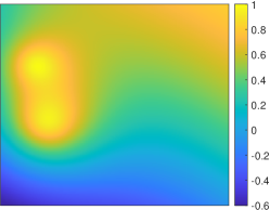
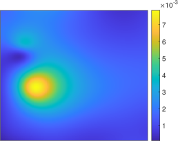
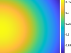
The difference between Helmholtz and Poisson cases lies in the fact that the former is complex-valued. We again assume a known number of point sources, and employ points in and points on to form the empirical loss . We use two 3-20-20-20-1 NNs to approximate the real and imaginary parts of the regular part , take the penalty weights , and set the learning rate to 1.0e-3 for and 2.0e-3 for . The training results after 10,000 iterations are shown in Table 5 and Fig. 4 for the noise level . Fig. 4 shows the real and imaginary parts of sliced at . The pointwise error is small. For partial Cauchy data, the recovered intensities and locations are still satisfactory, cf. Table 5. This again shows the capability of SENN for identifying point sources.
| point | ||||||
| exact | 5.000 | 2.000 | -3.000 | |||
| (i) | 5.016 | 1.999 | -3.022 | |||
| (ii) | 5.009 | 2.006 | -3.026 |
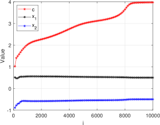
Fig. 5 shows the dynamics of the loss and the relative error during the training process. We observe from Figs. 5(a) that the decay of the loss accelerates after around 400 iterations. This coincides with Fig. 5(b), where the location of one of the points converges, as indicated by the intersection of the iteration trajectory. Like in Example 4.1, after 5,000 iterations, the iteration still exhibits oscillations in both loss curve and relative error, akin to the catapult phenomenon in deep learning.
 |
 |
 |
 |
 |
 |
| (a) exact | (b) predicted | (c) error |
 |
 |
 |
| (a) vs | (b) point 3 | (c) vs |
Last, we give one example with a variable coefficient.
Example 4.4.
Consider the following second-order elliptic equation with a variable coefficient: in with . The information of the source is shown in Table 6.
| point | density | location | density | location |
| exact | 10.000 | 10.000 | ||
| 9.726 | 10.172 | |||
| 9.717 | 10.240 | |||
| 9.703 | 10.287 |
We equip the equation with a Neumann boundary condition on , and fix in order to ensure the uniqueness of the direct problem. Since the exact solution is unavailable, we solve the direct problem using the Galerkin finite element method (FEM) first and then use the Dirichlet data to detect the sources. In order to get accurate data, we use the singularity splitting strategy [21, 24] by splitting the solution into and approximating using the FEM. Due to the presence of the variable coefficient , the direct method in [16] no longer works. The numerical results in Table 6 show that the method works equally well for the variable coefficient , which shows its versatility for more general problems.
5 Conclusions
In this work, we have developed a novel neural network based algorithm to identify point sources in the Poisson equation from Cauchy data. It employs the fundamental solution of the elliptic operator to extract the singular part of the solution and neural networks to approximate the regular part, and to estimate the solution (state) and unknown parameters of the point sources by optimizing an empirical loss. We have also derived an error estimate for the method. This is achieved by first establishing Hölder conditional stability for the recovered sources and densities, and the solution of the differential equation in terms of the loss function, and then deriving a priori bound on the empirical loss using techniques in statistical learning theory. We presented several numerical experiments to show its performance, which show satisfactory recovery for point sources and excellent stability with respect to noise.
There are several directions for further research. First, it is of interest to extend the approach to more general sources, e.g., that concentrate on lines, curves or surfaces, which is prevalent in biological modeling, and to develop relevant theoretical analysis, including partial boundary data. Second, it is important to analyze other types of sources, e.g., dipoles or mixture of monopoles and dipoles, or more general distributed sources. Last, it is important to study other type of mathematical models, e.g., parabolic or hyperbolic systems, which correspond to the nonstationary counterpart of the elliptic case and potentially involve time-dependent intensities and moving locations.
Appendix A Technical estimates
To bound the terms in the splitting (3.23), we employ Rademacher complexity of the function classes , and . Rademacher complexity [2, 3] measures the complexity of a collection of functions by the correlation between function values with Rademacher random variables, i.e., with probability .
Definition A.1.
Let be a real-valued function class defined on the domain and be i.i.d. samples from a distribution . Then the Rademacher complexity of is defined by
where are i.i.d Rademacher random variables.
We have the following PAC-type generalization bound [38, Theorem 3.1].
Lemma A.1.
Let be a set of i.i.d. random variables, and let be a function class defined on such that . Then for any , with probability at least :
Next, we state Dudley’s lemma ([35, Theorem 9], [42, Theorem 1.19]), which bounds Rademacher complexities using covering number.
Definition A.2.
Let be a metric space of real valued functions, and . A set is called an -cover of if for any , there exists an element such that . The -covering number is the minimum cardinality among all -covers of with respect to .
Lemma A.2.
Let be a real-valued function class defined on the domain , , and the covering number of . Then is bounded by
To apply Lemma A.1, we bound the Rademacher complexities , and . This follows from Dudley’s formula in Lemma A.2. The next lemma gives useful boundedness and Lipschitz continuity of the NN function class in terms of ; see [29, Lemma 3.4 and Remark 3.3] and [11, Lemma 5.3]. These estimates also hold when is replaced with . The condition is used in deriving the bounds in Lemma A.3.
Lemma A.3.
Let , and be the depth, width and maximum weight bound of an NN function class , with nonzero weights. Then for any , the following estimates hold
-
(i)
, ;
-
(ii)
, ;
-
(iii)
, .
Next we give boundedness and Lipschitz continuity of functions in , and .
Lemma A.4.
There exists a constant such that for all ; for all ; for all . Moreover, the following Lipschitz continuity estimates hold: (i) for all ; (ii) for all ; (iii) for all .
References
- [1] Y. E. Anikonov, B. A. Bubnov, and G. N. Erokhin. Inverse and Ill-posed Sources Problems. Walter de Gruyter, Berlin, 2013.
- [2] M. Anthony and P. L. Bartlett. Neural Network Learning: Theoretical Foundations. Cambridge University Press, Cambridge, 1999.
- [3] P. L. Bartlett and S. Mendelson. Rademacher and Gaussian complexities: risk bounds and structural results. J. Mach. Learn. Res., 3:463–482, 2002.
- [4] M. Berggren. Approximations of very weak solutions to boundary-value problems. SIAM J. Numer. Anal., 42(2):860–877, 2004.
- [5] L. Bottou, F. E. Curtis, and J. Nocedal. Optimization methods for large-scale machine learning. SIAM Rev., 60(2):223–311, 2018.
- [6] R. H. Byrd, P. Lu, J. Nocedal, and C. Y. Zhu. A limited memory algorithm for bound constrained optimization. SIAM J. Sci. Comput., 16(5):1190–1208, 1995.
- [7] Z. Cai and S. Kim. A finite element method using singular functions for the Poisson equation: corner singularities. SIAM J. Numer. Anal., 39(1):286–299, 2001.
- [8] Z. Cai, S. Kim, and B.-C. Shin. Solution methods for the Poisson equation with corner singularities: numerical results. SIAM J. Sci. Comput., 23(2):672–682, 2001.
- [9] M. Chafik, A. El Badia, and T. Ha-Duong. On some inverse EEG problems. In Inverse Problems in Engineering Mechanics II, pages 537–544. Elsevier, 2000.
- [10] F. Cucker and S. Smale. On the mathematical foundations of learning. Bull. Amer. Math. Soc. (N.S.), 39(1):1–49, 2002.
- [11] Y. Dai, B. Jin, R. Sau, and Z. Zhou. Solving elliptic optimal control problems via neural networks and optimality system. Preprint, arXiv:2308.11925, 2023.
- [12] H. Du, Z. Li, J. Liu, Y. Liu, and J. Sun. Divide-and-conquer DNN approach for the inverse point source problem using a few single frequency measurements. Inverse Problems, 39(11):115006, 19, 2023.
- [13] A. El Badia and A. El Hajj. Hölder stability estimates for some inverse pointwise source problems. C. R. Math. Acad. Sci. Paris, 350(23-24):1031–1035, 2012.
- [14] A. El Badia and A. El Hajj. Stability estimates for an inverse source problem of Helmholtz’s equation from single Cauchy data at a fixed frequency. Inverse Problems, 29(12):125008, 20, 2013.
- [15] A. El Badia and T. Ha-Duong. Some remarks on the problem of source identification from boundary measurements. Inverse Problems, 14(4):883–891, 1998.
- [16] A. El Badia and T. Ha-Duong. An inverse source problem in potential analysis. Inverse Problems, 16(3):651–663, 2000.
- [17] L. C. Evans. Partial Differential Equations. AMS, Providence, RI, second edition, 2010.
- [18] G. J. Fix, S. Gulati, and G. I. Wakoff. On the use of singular functions with finite element approximations. J. Comput. Phys., 13:209–228, 1973.
- [19] T.-P. Fries and T. Belytschko. The extended/generalized finite element method: an overview of the method and its applications. Internat. J. Numer. Methods Engrg., 84(3):253–304, 2010.
- [20] W. Gautschi. On inverses of Vandermonde and confluent Vandermonde matrices. Numer. Math., 4:117–123, 1962.
- [21] I. G. Gjerde, K. Kumar, J. M. Nordbotten, and B. Wohlmuth. Splitting method for elliptic equations with line sources. ESAIM: Math. Model. Numer. Anal., 53(5):1715–1739, 2019.
- [22] M. Grüter and K.-O. Widman. The Green function for uniformly elliptic equations. Manuscripta Math., 37(3):303–342, 1982.
- [23] I. Guhring and M. Raslan. Approximation rates for neural networks with encodable weights in smoothness spaces. Neural Networks, 134:107–130, 2021.
- [24] T. Hu, B. Jin, and Z. Zhou. Solving elliptic problems with singular sources using singularity splitting deep Ritz method. SIAM J. Sci. Comput., 45(4):A2043–A2074, 2023.
- [25] T. Hu, B. Jin, and Z. Zhou. Solving Poisson problems in polygonal domains with singularity enriched physics informed neural networks. SIAM J. Sci. Comput., 46(4):C369–C398, 2024.
- [26] M. Ikehata. Reconstruction of obstacles from boundary measurements. Wave Motion, 30(3):205–223, 1999.
- [27] V. Isakov. Inverse Source Problems. AMS, Providence, RI, 1990.
- [28] Y. Jiao, Y. Lai, D. Li, X. Lu, F. Wang, Y. Wang, and J. Z. Yang. A rate of convergence of physics informed neural networks for the linear second order elliptic PDEs. Commun. Comput. Phys., 31(4):1272–1295, 2022.
- [29] B. Jin, X. Li, and X. Lu. Imaging conductivity from current density magnitude using neural networks. Inverse Problems, 38(7):075003, 36, 2022.
- [30] G. E. Karniadakis, I. G. Kevrekidis, L. Lu, P. Perdikaris, S. Wang, and L. Yang. Physics-informed machine learning. Nature Rev. Phys., 3:422–440, 2021.
- [31] D. P. Kingma and J. Ba. Adam: A method for stochastic optimization. In 3rd International Conference for Learning Representations, San Diego, 2015.
- [32] G. Kriegsmann and W. Olmstead. Source identification for the heat equation. Appl. Math. Lett., 1(3):241–245, 1988.
- [33] P. Li, Y. Liang, and Y. Wang. A data-assisted two-stage method for the inverse random source problem. SIAM J. Imaging Sci., 16(4):1929–1952, 2023.
- [34] Y. Lu, H. Chen, J. Lu, L. Ying, and J. Blanchet. Machine learning for elliptic PDEs: Fast rate generalization bound, neural scaling law and minimax optimality. In International Conference on Learning Representations, 2022.
- [35] Y. Lu, J. Lu, and M. Wang. A priori generalization analysis of the deep Ritz method for solving high dimensional elliptic partial differential equations. In Conference on Learning Theory, pages 3196–3241. PMLR, 2021.
- [36] C. M. Michel, G. Lantz, L. Spinelli, R. G. De Peralta, T. Landis, and M. Seeck. 128-channel EEG source imaging in epilepsy: clinical yield and localization precision. J. Clinical Neurophys., 21(2):71–83, 2004.
- [37] C. M. Michel, M. M. Murray, G. Lantz, S. Gonzalez, L. Spinelli, and R. Grave de Peralta. EEG source imaging. Clinical Neurophys., 115(10):2195–2222, 2004.
- [38] M. Mohri, A. Rostamizadeh, and A. Talwalkar. Foundations of Machine Learning. MIT Press, Cambridge, MA, 2018.
- [39] R. Rado. Factorization of even graphs. Quart. J. Math., os-20(1):95–104, 1949.
- [40] J. Sirignano and K. Spiliopoulos. Dgm: A deep learning algorithm for solving partial differential equations. J. Comput. Phys., 375:1339–1364, 2018.
- [41] S. Wang, X. Yu, and P. Perdikaris. When and why PINNs fail to train: a neural tangent kernel perspective. J. Comput. Phys., 449:110768, 28, 2022.
- [42] M. M. Wolf. Mathematical Foundations of Supervised Learning. Lecture notes, available at https://www-m5.ma.tum.de/foswiki/pub/M5/Allgemeines/MA4801_2021S/ML.pdf (accessed on Feb. 1, 2023), 2021.
- [43] H. Zhang and J. Liu. Solving an inverse source problem by deep neural network method with convergence and error analysis. Inverse Problems, 39(7):075013, 2023.
- [44] M. Zhang, Q. Li, and J. Liu. On stability and regularization for data-driven solution of parabolic inverse source problems. J. Comput. Phys., 474:111769, 20, 2023.