Learning to Explore for Stochastic Gradient MCMC

Abstract

Bayesian Neural Networks (bnns) with high-dimensional parameters pose a challenge for posterior inference due to the multi-modality of the posterior distributions. Stochastic Gradient Markov Chain Monte Carlo (sgmcmc) with cyclical learning rate scheduling is a promising solution, but it requires a large number of sampling steps to explore high-dimensional multi-modal posteriors, making it computationally expensive. In this paper, we propose a meta-learning strategy to build sgmcmc which can efficiently explore the multi-modal target distributions. Our algorithm allows the learned sgmcmc to quickly explore the high-density region of the posterior landscape. Also, we show that this exploration property is transferrable to various tasks, even for the ones unseen during a meta-training stage. Using popular image classification benchmarks and a variety of downstream tasks, we demonstrate that our method significantly improves the sampling efficiency, achieving better performance than vanilla sgmcmc without incurring significant computational overhead.

1 Introduction

Bayesian methods have received a lot of attention as powerful tools for improving the reliability of machine learning models. Bayesian methods are gaining prominence due to their ability to offer probability distributions over model parameters, thereby enabling the quantification of uncertainty in predictions. They find primary utility in safety-critical domains like autonomous driving, medical diagnosis, and finance, where the accurate modeling of prediction uncertainty often takes precedence over the predictions themselves. The integration of Bayesian modeling with (deep) neural networks, often referred to as Bayesian Neural Networks (bnns), introduces exciting prospects for the development of secure and trustworthy decision-making systems.

However, there are significant problems for the successful application of bnns in real-world scenarios. Bayesian inference in high-dimensional parameter space, especially for deep and large models employed for the applications mentioned above, is notoriously computationally expensive and often intractable due to the complexity of the posterior distribution. Moreover, posterior landscapes of bnns frequently display multi-modality, where multiple high density regions exist, posing a significant challenge to efficient exploration and sampling. Due to this difficulty, the methods that are reported to work well for relatively small models, for instance, variational inference (Blei & McAuliffe, 2017) or Hamiltonian Monte Carlo (hmc) (Neal et al., 2011), can severly fail for deep neural networks trained with large amount of data, when applied without care.

Recently, Stochastic Gradient Markov Chain Monte Carlo (sgmcmc) methods (Welling & Teh, 2011; Chen et al., 2014; Ma et al., 2015) have emerged as powerful tools for enhancing the scalability of approximate Bayesian inference. This advancement has opened up the possibilities of applying Bayesian methods to large-scale machine learning tasks. sgmcmc offers a versatile array of methods for constructing Markov chains that converge towards the target posterior distributions. The simulation of these chains primarily relies on stochastic gradients, making them particularly suitable for bnns trained on large-scale datasets. However, despite the notable successes of sgmcmc in some bnn applications (Welling & Teh, 2011; Chen et al., 2014; Ma et al., 2015; Zhang et al., 2020), there remains a notable challenge. Achieving optimal performance often demands extensive engineering efforts and hyperparameter tuning. This fine-tuning process typically involves human trial and error or resource-intensive cross-validation procedures. Furthermore, it’s worth noting that even with the use of sgmcmc methods, there remains room for improvement in efficiently exploring multi-modal posterior distributions. As a result, in practical applications, a trade-off between precision and computational resources often becomes necessary.

To address these challenges, we introduce a novel meta-learning framework tailored to promote the efficient exploration of sgmcmc algorithms. Traditional sgmcmc methods often rely on handcrafted design choices inspired by mathematical or physics principles. Recognizing the pivotal role these design components play in shaping the trade-off between exploration and exploitation within sgmcmc chains, we argue in favor of learning them directly from data rather than manually specifying them. To achieve this, we construct neural networks to serve as meta-models responsible for approximating the gradients of kinetic energy terms. These meta-models are trained using a diverse set of bnns inference tasks, encompassing various datasets and architectural configurations. Our proposed approach, termed Learning to Explore (l2e), exhibits several advantageous properties, including better mixing rates, improved prediction performance, and a reduced need for laborious hyperparameter tuning.

Our contributions can be summarized as follows:

• We introduce l2e, a novel meta-learning framework enhancing sgmcmc methods. In contrast to conventional hand-designed approaches and meta-learning approach (Gong et al., 2018), l2e learns the kinetic energy term directly, offering a more data-driven and adaptable solution.

• We present a multitask training pipeline equipped with a scalable gradient estimator for l2e. This framework allows the meta-learned sgmcmc techniques to generalize effectively across a wide range of tasks, extending their applicability beyond the scope of tasks encountered during meta-training.

• Using real-world image classification benchmarks, we demonstrate the remarkable performance of bnns inferred using the sgmcmc algorithm discovered by l2e, both in terms of prediction accuracy and sampling efficiency.

2 Backgrounds

2.1 sgmcmc for Bayesian Neural Networks

Settings.

In this paper, we focus on supervised learning problems with a training dataset ${\mathcal{D}}=\{(x_{i},y_{i})_{i=1}^{n}$ with $x_{i}$ being observation and $y_{i}$ being label. Given a neural network with a parameter $\theta\in\mathbb{R}^{d}$, a likelihood $p(y\,|\,x,\theta)$ and a prior $p(\theta)$ are set up, together defining an energy function $U(\theta)=-\sum_{i=1}^{n}\log p(y_{i}\,|\,x_{i},\theta)-\log p(\theta)$. The goal is to infer the posterior distribution $p(\theta\,|\,{\mathcal{D}})\propto\exp(-U(\theta))$. When the size of the dataset $n$ is large, evaluating the energy function $U(\theta)$ or its gradient $\nabla_{\theta}U(\theta)$ may be undesirably costly as they require a pass through the entire dataset ${\mathcal{D}}$. For such scenarios, sgmcmc (Welling & Teh, 2011; Chen et al., 2014; Ma et al., 2015) is a standard choice, where the gradients of the energy function $\nabla_{\theta}U(\theta)$ are approximated by a stochastic gradient computed from mini-batches. That is, given a mini-batch $B\subset\{1,\dots,n\}$ where $|B|\ll n$, an unbiased estimator of the full gradient $\nabla_{\theta}U(\theta)$ with $B$ can be computed as

$$\nabla_{\theta}\tilde{U}(\theta)=-\frac{n}{|B|}\sum_{i\in B}\nabla_{\theta}\log p(y_{i}\,|\,x_{i},\theta)-\nabla_{\theta}\log p(\theta)$$

A complete recipe.

There may be several ways to build a Markov chain leading to the target posterior distribution. Ma et al. (2015) presented a generic recipe that includes all the convergent sgmcmc algorithms as special cases, constituting a complete framework. In this recipe, a parameter $\theta$ of interest is augmented with an auxiliary momentum variable $r$, and an Stochastic Differential Equation (sde) of the following form is defined for a joint variable $z=(\theta,r)\in\mathbb{R}^{2d}$ as follows.

$$\mathrm{d}z=\left[-(D(z)+Q(z))\nabla_{z}H(z)+\Gamma(z)\right]\mathrm{d}t$$ (1)

$$+\sqrt{2D(z)}\mathrm{d}w_{t}$$

$$H(z):=U(\theta)+g(\theta,r)$$

$$\Gamma_{i}(z):=\sum_{j=1}^{2d}\frac{\partial}{\partial z_{j}}(D_{ij}(z)+Q_{ij}(z)),$$

where $g(\theta,r)$ is the conditional energy function of the momentum $r$ such that $p(z)\propto\exp(-H(z))$ and $w_{t}$ is $2d$-dimensional Brownian motion. Here, $D(z)\in\mathbb{R}^{2d\times 2d}$ and $Q(z)\in\mathbb{R}^{2d\times 2d}$ are restricted to be positive semi-definite and skew-symmetric, respectively. Given this sde, one can obtain a sgmcmc algorithm by first substituting the full gradient $\nabla_{z}H(z)$ with a mini-batch gradient $\nabla_{z}\tilde{H}(z)=\nabla_{z}(\tilde{U}(\theta)+g(\theta,r))$ and then discretizing it via a numerical solver such as sympletic Euler method. A notable example would be Stochastic Gradient Hamiltonian Monte Carlo (sghmc) (Chen et al., 2014), where $g(\theta,r)=\frac{1}{2}r^{\top}M^{-1}r$, $D(z)=\begin{bmatrix}0&0\\ 0&C\end{bmatrix}$, and $Q(z)=\begin{bmatrix}0&-I\\ I&0\end{bmatrix}$ for some positive semi-definite matrices $M$ and $C$, leading to an algorithm when discretized with symplectic Euler method as follows.

$$r_{t+1}=r_{t}-\epsilon_{t}\nabla\tilde{U}(\theta_{t})-\epsilon_{t}CM^{-1}r_{t}+\xi_{t}$$ (2)

$$\theta_{t+1}=\theta_{t}+\epsilon_{t}M^{-1}r_{t+1},$$

where $\xi_{t}\sim{\mathcal{N}}(0,2C\epsilon_{t})$ and $\epsilon_{t}$ is a step-size.

The complete recipe includes interesting special cases that introduce adaptive preconditioners to improve the mixing of sgmcmc (Girolami & Calderhead, 2011; Li et al., 2016; Wenzel et al., 2020). For instance, Li et al. (2016) proposed Preconditioned Stochastic Gradient Langevin Dynamics (psgld), which includes RMSprop (Tieleman & Hinton, 2012)-like preconditioning matrix in the updates:

$$\theta_{t+1}=\theta_{t}-\epsilon_{t}[G(\theta_{t})\nabla_{\theta}\tilde{U}(\theta)+\Gamma(\theta_{t})]+\xi_{t}$$ (3)

$$V(\theta_{t+1})=\alpha V(\theta_{t})+(1-\alpha)\frac{\nabla_{\theta}\tilde{U}(\theta_{t})}{n}\odot\frac{\nabla_{\theta}\tilde{U}(\theta_{t})}{n}$$

$$G(\theta_{t+1})=\mathrm{diag}(\mathbf{1}\oslash(\lambda\mathbf{1}+\sqrt{V(\theta_{t+1})}),$$

where $\xi_{t}\sim{\mathcal{N}}(0,2G(\theta_{t})\epsilon_{t})$ and $\oslash,\odot$ denotes elementwise division and multiplication, respectively. psgld exploits recent gradient information to adaptively adjust the scale of energy gradients and noise. However, this heuristical adjustment is still insufficient to efficiently explore the complex posteriors of bnns (Zhang et al., 2020).

Recently, Zhang et al. (2020) introduced cyclic learning rate schedule for efficient exploration of multi-modal distribution. The key idea is using the spike of learning rate induced by cyclic learning rate to escape from a single mode and move to other modes. However, in our experiment, we find that sgmcmc with cyclical learning rate does not necessarily capture multi-modality and it also requires a large amount of update steps to move to other modes in practice.

Prediction via Bayesian model averaging.

After inferring the posterior $p(\theta\,|\,{\mathcal{D}})$, for a test input $x_{*}$, the posterior predictive is computed as

$$p(y_{*}\,|\,x_{*},{\mathcal{D}})=\int_{\mathbb{R}^{d}}p(y_{*}\,|\,x_{*},\theta)p(\theta\,|\,{\mathcal{D}})\mathrm{d}\theta,$$ (4)

which is also referred to as Bayesian Model Averaging (bma). In our setting, having collected from the posterior samples $\theta_{1},\dots,\theta_{K}$ from a convergent chain simulated from sgmcmc procedure, the predictive distribution is approximated with a Monte-Carlo estimater,

$$p(y_{*}\,|\,x_{*},{\mathcal{D}})\approx\frac{1}{K}\sum_{k=1}^{K}p(y_{*}\,|\,x_{*},\theta_{k}).$$ (5)

As one can easily guess, the quality of this approximation depends heavily on the quality of the samples drawn from Markov Chain Monte Carlo (mcmc) procedure. For over-parameterzied deep neural networks that we are interested in, the target posterior $p(\theta\,|\,{\mathcal{D}})$ is typically highly multi-modal, so simple sgmcmc methods suffer from poor mixing; that is, the posterior samples collected from those methods are not widely spread throughout the parameter space, so it takes exponentially many samples to achieve desired level of accuracy for the approximation. Hence, a good sgmcmc algorithm should be equipped with the ability to efficiently explore the parameter space, while still be able to stay sufficiently long in high-density regions. That is, it should have a right balance between exploration-exploitation.

Meta Learning

Meta-learning, or learning to learn, refers to the algorithm that learns the useful general knowledge from source tasks that can transfer to the unseen tasks. Most meta-learning algorithms involves two levels of learning: an inner-loop and outer-loop (Metz et al., 2018). Inner-loop usually contains the training procedure of particular task. In our work, inner-loop for our meta-training is iteratively update the model parameter $\theta$ by running sgmcmc with learnable transition kernel. Outer-loop refers to the training procedure of meta-parameter $\phi$, which is done by minimizing meta-objective $L(\phi)$.

Meta Learning and MCMC

There exists line of work that parameterize the transition kernel of MCMC with trainable function for various purposes. Levy et al. (2017) used learnable invertible operator to automatically design the transition kernel of HMC for good mixing. For sgmcmc, Gong et al. (2018) parameterized the curl matrix and acceleration matrix using neural networks under the framework of Ma et al. (2015). Although Gong et al. (2018) is the closest work for our method, this work did not verified its task generalization, i.e., evaluated only on the dataset that was used for training. Moreover, the scale of the experiments in Gong et al. (2018) are limited to small-sized network architectures. We further demonstrate the limitation of Gong et al. (2018) in simulating large scale multi-modal bnns posterior, along with detailed discussions in Appendix E. To the best of our knowledge, our work firstly proposes the method to meta-learn sgmcmc that can generalize to unseen datasets and scale to large-scale bnns.

Limitation of Meta-sgmcmc (Gong et al., 2018)

Meta-sgmcmc aims to learn the diffusion matrix $D(z)$ and the curl matrix $Q(z)$ in LABEL:eq:sgmcmc_recipe to build a sgmcmc algorithm that can quickly converge to a target distribution. For this purpose, neural network $D_{f}(z)$ and $Q_{f}(z)$ are employed to model $D(z)$ and $Q(z)$. We point out that this parameterization has notable limitations, especially in terms of efficient exploration of high-dimensional multi-modal target distribution.

• According to the recipe in LABEL:eq:sgmcmc_recipe, the diffusion and the curl that are dependent on $z$ involves the additional correction term $\Gamma(z)$. This hurts the scalability of the algorithm, as computing $\Gamma(z)$ involves computing the gradient of $D_{f}(z)$ and $Q_{f}(z)$ with respect to $z$. This amounts to a significant computational burden as the dimension of $z$ increases and involves finite-difference approximation. While Meta-sgmcmc attempted to address this issue of computational cost through finite difference, but it still introduces additional computation with time complexity $O(HD)$ where $H$ is number of hidden units of neural network in meta-sampler and $D$ is dimension of $\theta$. Also, it is important to note that adding such approximation can negatively impact the convergence of the sampler.

• The objective function of Meta-sgmcmc is the KL divergence between the target distribution and the distribution of the samples obtained from the Meta-sgmcmc chain. This objective is not computed in closed-from and nor its gradient. Gong et al. (2018) proposes to use Stein gradient estimator (Li & Turner, 2018) which is generally hard to tune. Moreover, Gong et al. (2018) uses Truncated BackPropagation Through Time (tbptt) for the gradient estimation, which is a biased estimator of the true gradient, and limited in the length of the inner step for meta-learning due to the memory consumption.

3 Main contribution: Learning to Explore

3.1 Overcome the limitations of Meta-sgmcmc

To avoid aforementioned limitations of Meta-sgmcmc, we newly design the meta-learning method for sgmcmc as follows:

• We parameterize the gradients of the kinetic energy function and keep $D_{f}(z)$ and $Q_{f}(z)$ independent of $z$. We can avoid the additional computational cost of computing $\Gamma(z)$ without sacrificing the flexibility of the sampler.

• We use a new meta-objective called bma meta-loss which is the Monte-Carlo estimator of the predictive distribution to enhance the exploration and performance of the learned sampler. Both of our meta-objective and its gradient can be computed in closed-form. Also, we employ Evolution Strategy (es) (Salimans et al., 2017; Metz et al., 2019) for gradient estimation, which is an unbiased estimator of the true meta-gradient. This also consumes significantly less memory compared to analytic gradient methods, allowing us to keep the length of the inner-loop much longer during meta-learning.

3.2 Meta-learning framework for sgmcmc

Instead of using a hand-designed recipe for sgmcmc, we aim to learn the proper sgmcmc update steps through meta learning. The existing works, both the methods using hand-designed choices or meta-learning (Gong et al., 2018), try to determine the forms of the matrices $D(z)$ and $Q(z)$ while keeping the kinetic energy $g(\theta,r)$ as simple Gaussian energy function, that is, $g(\theta,r)=r^{\top}M^{-1}r/2$. This choice indeed is theoretically grounded, which can be shown to be optimal when the target distribution is Gaussian (Betancourt, 2017), but may not be optimal for the complex multi-modal posteriors of bnns. We instead choose to learn $g(\theta,r)$ while keeping $D(z)$ and $Q(z)$ as simple as possible. We argue that the meta-learning approach based on this alternative parameterization is more effective in learning versatile sgmcmc procedure that scales to large bnns.

More specifically, we parameterize the gradients of the kinetic energy function $\nabla_{\theta}g(\theta,r)$ and $\nabla_{r}g(\theta,r)$ with neural networks $\alpha_{\phi}(\theta,r)$ and $\beta_{\phi}(\theta,r)$ respectively, and set $D(z)$ and $Q(z)$ as in sghmc. The update step of sgmcmc, when discretized with symplectic Euler method is,

$$r_{t+1}=r_{t}-\epsilon_{t}[\nabla_{\theta}\tilde{U}(\theta_{t})+\alpha_{\phi}(\theta_{t},r_{t})+C\beta_{\phi}(\theta_{t},r_{t})]+\xi_{t}$$ (6)

$$\theta_{t+1}=\theta_{t}+\epsilon_{t}\beta_{\phi}(\theta_{t},r_{t+1}).$$

where $\xi_{t}\sim{\mathcal{N}}(0,2C\epsilon_{t})$. Since we parameterize $\nabla g(\theta,r)$ and do not explicitly define the form of $g(\theta,r)$, we make the following assumptions about the underlying function $g(\theta,r)$.

Assumption 3.1.

There exists an energy function $g(\theta,r)$ whose gradients with respect to $\theta,r$ are $\alpha_{\phi}(\theta,r)$ and $\beta_{\phi}(\theta,r)$ respectively, and $\int\exp(-g(\theta,r))dr=\text{constant}.$

We also present another version of l2e which does not require additional assumptions in Appendix D. The neural networks $\alpha_{\phi}$ and $\beta_{\phi}$ are parameterized as two-layer Multi-Layer Perceptrons (mlps) with 32 hidden units. Specifically, $\alpha_{\phi}$ and $\beta_{\phi}$ are applied to each dimension of parameter and momentum independently, similar to the commonly used learned optimizers (Andrychowicz et al., 2016; Metz et al., 2019). Again, following the common literature in learned optimizers (Metz et al., 2019), for each dimension of the parameter and momentum, we feed the corresponding parameter and momentum values, the stochastic gradients of energy functions for that element, and running average of the gradient at various time scales, as they are reported to encode the sufficient information about the loss surface geometry. See Appendix I for implementation details of $\alpha_{\phi}$ and $\beta_{\phi}$. By leveraging this information, we expect our meta-learned sgmcmc procedure to capture the multi-modal structures of the target posteriors of bnns, and thus yielding a better mixing method.

3.3 Meta-Objective and Optimization

Objective functions for meta-learning.

Meta-objective should reflect the meta-knowledge one wants to learn. We design the meta-objective based on the hope that samples collected through sgmcmc should be good at approximating the posterior predictive $p(y_{*}|x_{*},{\mathcal{D}})$. In order to achieve this goal, we propose the meta-objective called bma meta-loss. After the sufficient number of inner-updates, we collect $K$ parameter samples with some interval between them (thinning). Let $\theta_{k}(\phi)$ be the $k^{th}$ collected parameter, and we compute the Monte-Carlo estimator of the predictive distribution and use it as a meta-objective function (note the dependency of $\theta_{k}$ on the meta-parameter $\phi$, as it is a consequence of learning sgmcmc with the meta-parameter $\phi$).

$$L(\phi)=-\log\frac{1}{K}\sum_{k=1}^{K}p(y_{*}\,|\,x_{*},\theta_{k}(\phi)),$$ (7)

where $(x_{*},y_{*})$ is a validation data point.

1:  Input: Task distribution $P(\mathcal{T})$, inner iterations $N_{\text{inner}}$, outer iterations $N_{\text{outer}}$, step size $\epsilon$, noise scale $\sigma^{2}$, initial meta-parameter $\phi_{0}$.

2:  Output: Meta parameter $\phi$.

3:  for $j=1,\dots,N_{\text{outer}}$ do

4:     Sample task $T_{i}\sim P(\mathcal{T})$

5:     Initialize model parameter $\theta_{0}$ for $T_{i}$

6:     Sample $\eta\sim{\mathcal{N}}(0,\sigma^{2}I)$

7:     $L(\phi+\eta)\leftarrow\text{InnerLoop}(\theta_{0},\phi+\eta,\epsilon,N_{\text{inner}})$

8:     $L(\phi-\eta)\leftarrow\text{InnerLoop}(\theta_{0},\phi-\eta,\epsilon,N_{\text{inner}})$

9:     $\nabla_{\phi}L\leftarrow\frac{1}{2\,\sigma^{2}}\eta\,(L(\phi+\eta)-L(\phi-\eta))$

10:     $\phi\leftarrow\phi-\gamma\nabla_{\phi}L(\phi)$

11:  end for

Algorithm 1 Meta training procedure

Gradient estimation for meta-objective.

Estimating the meta-gradient $\nabla_{\phi}L(\phi)$ is highly non-trivial (Metz et al., 2018, 2019), especially when the number of inner update steps is large. For instance, a naïve method such as backpropagation through time would require memory grows linearly with the number of inner-steps, so become easily infeasible for even moderate sized models. One might consider using the truncation approximation, but that would result in a biased gradient estimator. Instead, we adapt es (Salimans et al., 2017) with antithetic sampling scheme, which has been widely used in recent literature of training learned optimizer. Metz et al. (2019) showed that unrolled optimization with many inner-steps can lead to chaotic meta-loss surface and es is capable of relieving this pathology by employing smoothed loss,

$$L(\phi)=\mathbb{E}_{\tilde{\phi}\sim{\mathcal{N}}(\phi,\sigma^{2}I)}\left[L(\tilde{\phi})\right]$$ (8)

where $\sigma^{2}$ determines the degree of smoothing. Also, antithetic sampling is usually applied to reduce the estimation variance of $\nabla_{\phi}L(\phi)$. Through log-derivative trick, we can get unbiased estimator of (8),

$$\hat{g}=\frac{1}{N}\sum_{i=1}^{N}L(\phi+\eta_{i})\frac{\eta_{i}}{\sigma^{2}}$$ (9)

where $\eta_{i}\overset{\mathrm{i.i.d}}{\sim}{\mathcal{N}}(0,\sigma^{2}I)$. In addition, we can get another unbiased estimator $\hat{g}^{-1}=-\frac{1}{N}\sum_{i=1}^{N}L(\phi-\eta_{i})\frac{\eta_{i}}{\sigma^{2}}$ by reusing the negative of $\eta_{i}$. By taking the average of two estimators, we can obtain the following gradient estimator.

$$\hat{\nabla}_{\phi}L(\phi)=\frac{1}{N}\sum_{i=1}^{N}\left[\frac{L(\phi+\eta_{i})-L(\phi-\eta_{i})}{2\sigma^{2}}\right]\eta_{i}$$ (10)

The estimator is also amenable to parallelization, improving the efficiency of gradient computation.

3.4 Meta training procedure

Generic pipeline.

General process of meta-training is as follows. First, for each inner-loop, we sample a task from the pre-determined task distribution. An inner-loop starts from an randomly initialized parameter and iteratively apply update step (6) to run a single chain of sgmcmc. Please refer to Algorithm 2 for detailed description. In the initial stage of meta-training, the chains from these inner loops show poor convergence, but the performance improves as training progresses. Similar to general Bayesian inference, we consider the early part of the inner loop as a burn-in period and collect samples from the end of the inner-loop at regular intervals when evaluating the meta-objective. This training process naturally integrates the meta-learning and Bayesian inference in that mimicking the actual inference procedure of Bayesian methods in realistic supervised learning tasks. In Figure 1 we show that l2e achieve desired level of accuracy for the approximation of posterior predictive with relatively small number of samples. This result indicates that l2e has successfully acquired the desired properties through meta-training.

Multitask training for better generalization.

In meta-learning, diversifying the task distribution is commonly known to enhance generalization. We include various neural network architectures and datasets in the task distribution to ensure that l2e has sufficient generalization capacity. Also, we evaluate how the task distribution diversity affects the performance of l2e in Table 11.

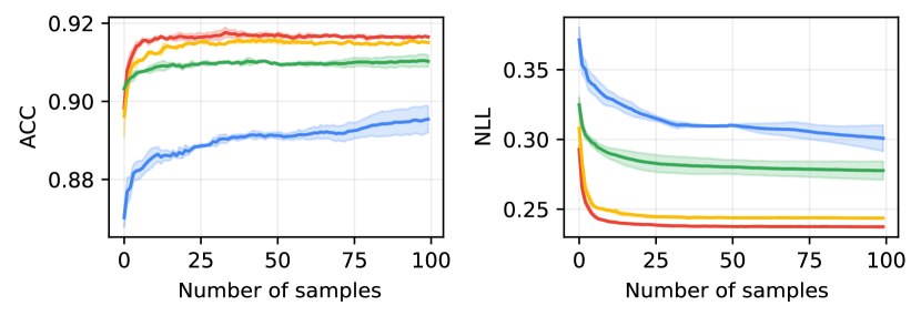
(a) fashion-MNIST (seen task)

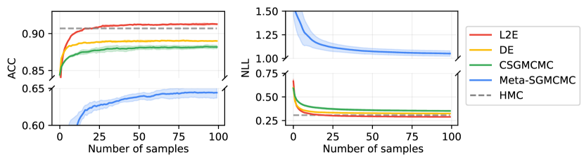
(b) CIFAR-10

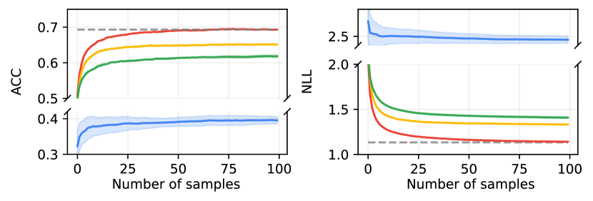
(c) CIFAR-100

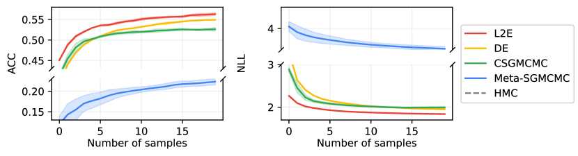
(d) Tiny-ImageNet

Figure 1: Predictive performance trend of each method as the number of samples for BMA increases. L2E exhibits superior predictive accuracy compared to other baseline methods. Note that only the fashion-MNIST dataset is included in meta-training task distribution. We also plot the performance of hmc reference samples from Izmailov et al. (2021b) as dashed line for CIFAR-10 and CIFAR-100. For meta-training details of Meta-sgmcmc, please refer to § I.4.

4 Experiments

In this section, we will evaluate the performance of l2e in various aspects. Through extensive experiments, we would like to demonstrate followings:

• l2e shows excellent performance on real-world image classification tasks and seamlessly generalizes to the tasks not seen during meta-training.

• l2e produces similar predictive distribution to hmc as well as good mixing of bnns posterior distribution in weight space.

• l2e can effectively explore and sample from bnns posterior distribution, collecting diverse set of parameters both in weight space and function space.

Experimental details

In this paragraph, we explain our experimental settings. We evaluate l2e and baseline methods on 4 datasets: fashion-MNIST (Xiao et al., 2017), CIFAR-10, CIFAR-100 (Krizhevsky et al., 2009) and Tiny-ImageNet (Le & Yang, 2015). Please refer to § K.1 for full experimental setup and details. We report the mean and standard deviation of results over three different trials. Code is available at https://github.com/ciao-seohyeon/l2e.

Comparing l2e with hmc

hmc is popular mcmc method since it can efficiently explore the target distribution and asymptotically converge to the target distribution, making it useful for inference in high-dimensional spaces. Due to its asymptotic convergence property, hmc often considered as golden standard in Bayesian Inference. However, its computational burden harms the applicability of hmc on modern machine learning tasks. Recently, Izmailov et al. (2021b) ran hmc on CIFAR-10 and CIFAR-100 datasets and released logits of hmc as reference. For deeper investigation of mixing of l2e, we compare l2e with hmc.

In order to compare the results with reference HMC samples from Izmailov et al. (2021b), we replicate the experimental setup of Izmailov et al. (2021b) including neural network architecture and dataset processing. The distinctive aspects of this setup are that they excluded data augmentation and replaced batch normalization layer in ResNet architecture to Filter Response Normalization (frn) (Singh & Krishnan, 2020) to remove stochasticity in evaluating posterior distribution. We use the ResNet20-FRN architecture with Swish activations (Ramachandran et al., 2017) and we use 40960 samples for training all methods. Also, we compare l2e to hmc 1-D synthetic regression experiments in Appendix G. We also provide experimental results with data augmentation in Appendix H with other discussions.

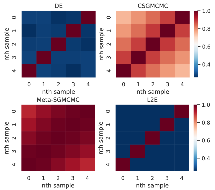
(a) Cosine similarity between weights.

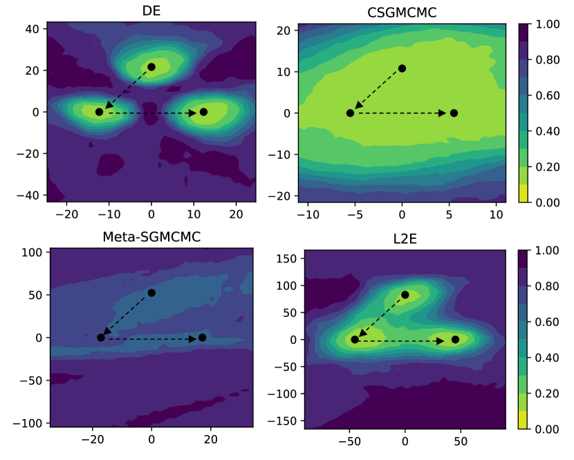
(b) Test error ($\%$) around the samples.

(c) Test error ($\%$) along linear path

Figure 2: Figures show multi-modality of various methods de, csgmcmc, Meta-sgmcmc and l2e with ResNet20-FRN on CIFAR-10. (a) shows cosine similarity between weights. (b) is loss surface as a function of model parameters in a 2-dimensional subspace spanned by solutions of each method. Colors represent the level of test error. (c) shows test error ($\%$) along linear path between a pair of parameters. Due to the inferior performance of Meta-sgmcmc, the offset of test error adjusted individually in CIFAR-10.

Task distribution for meta-training

We construct set of meta-training tasks using various datasets and model architectures. We use these tasks to meta-train meta-sgmcmc and l2e. Specifically, we use MNIST, fashion-MNIST, EMNIST (Cohen et al., 2017) and MedMNIST (Yang et al., 2021) as meta-training datasets. For model architecture, we fix the general structure with several convolution layers followed by readout MLP layer. For each outer training iteration, we randomly choose dataset and sample the configuration of architecture including number of channels, depth of the convolution layers and whether to use skip connections. See Appendix I for detailed configuration of task distribution. For evaluation, we use same meta-parameter of l2e and meta-sgmcmc for all experiments to check the generalization ability of each method.

4.1 Image classification results

Figure 1 illustrates the trend of predictive performance of each method as the number of samples for bma increases. We confirm that l2e outperforms other baselines in terms of predictive accuracy on completely unseen datasets and architectures during meta-training. Among datasets for evaluation, fashion-MNIST is the only dataset included in our task distribution. Despite not having seen other datasets during meta-training, l2e consistently outperforms other tuned baseline methods, showing that l2e can scale and generalize well to unseen larger tasks. Specifically, only de shows comparable predictive accuracy compared to l2e in fashion-MNIST dataset. In general, l2e shows rapid performance gain and outperforms other methods with relatively small number of samples. According to Figure 2, l2e collects diverse weights and functions and this diversity presumably affect the huge performance gain from bma.

On the other hand, Meta-sgmcmc exhibits poor predictive accuracy over all experiments. It converges very slowly compared to other methods and stucks in the low density region. This tendency gets worse when the evaluation task is significantly different from the distribution of meta-training tasks. In fashion-MNIST task, the performance of Meta-sgmcmc is still worse but relatively close to other methods than other tasks. Since learned sampler has seen fashion-MNIST dataset during meta-training, it adapts to this task to a moderate extent. However, it cannot produce even reasonable performance on other large scale tasks. We also evaluate l2e in the same experimental setup of Gong et al. (2018) and compare to the reported performance of Meta-sgmcmc in Appendix E. Without having seen CIFAR-10 dataset during meta-training, l2e significantly outperforms Meta-sgmcmc also in the experimental setup of Gong et al. (2018).

Table 1: Fidelity to predictive distribution given by hmc samples from Izmailov et al. (2021b).

Metric	Dataset	de	csgmcmc	l2e
Agreement	CIFAR-10	0.920$\scriptstyle{\pm 0.001}$	0.910$\scriptstyle{\pm 0.007}$	0.946$\scriptstyle{\pm 0.002}$
	CIFAR-100	0.751$\scriptstyle{\pm 0.001}$	0.726$\scriptstyle{\pm 0.007}$	0.771$\scriptstyle{\pm 0.003}$
Total Var	CIFAR-10	0.0103$\scriptstyle{\pm 0.0001}$	0.0108$\scriptstyle{\pm 0.0005}$	0.0075$\scriptstyle{\pm 0.0001}$
	CIFAR-100	0.0026$\scriptstyle{\pm 0.0000}$	0.0024$\scriptstyle{\pm 0.0001}$	0.0022$\scriptstyle{\pm 0.0000}$

4.2 Similarity to the hmc samples

As mentioned above, we compare l2e to hmc samples from Izmailov et al. (2021b) to objectively evaluate and investigate whether l2e has converged to target distribution. We measure the agreement between predictive distribution of hmc and l2e, and the difference of probability vector of two methods following Izmailov et al. (2021b). Please refer to Appendix K for details of metrics. In Table 1, we confirm that l2e makes higher fidelity approximation to predictive distribution of hmc than other baselines both in CIFAR-10 and CIFAR-100. This implies that L2E shows good mixing in function space by effectively capturing multi-modality of complex bnns posterior distribution. This high fidelity in predictive distribution can be attributed to the use of bma-loss as meta-objective.

Also, we conduct 1-D synthetic regression task to visually check whether l2e can capture the epistemic uncertainty similar to HMC. Figure 8 shows that l2e better captures “in-between" uncertainty than de. Although hmc captures epistemic uncertainty more effectively than l2e, we observe that l2e captures epistemic uncertainty in a similar manner to hmc. Please refer to Appendix G for details.

4.3 Capturing multi-modality

In Figure 2(c) and Figure 2(b), we observe the behavior of de, csgmcmc, and l2e in function space. In Figure 2(b), we display the test error surface using a 2-dimensional subspace spanned by the first three collected parameters for each method following Garipov et al. (2018). Parameters of de clearly located on multiple distinct modes as expected. In contrast, csgmcmc seems to sample parameters within a single mode, while samples from l2e appear to be in distinct modes. This aligns with the results from Fort et al. (2019) showing that csgmcmc has limited capability of capturing multi-modalities.

For deeper investigation, we plot test error along a linear path between multiple pairs of saved parameters inspired by Goodfellow et al. (2014). Existence of loss barrier in Figure 2(c) means the collected parameters belong to different modes. In Figure 2(c), l2e shows a significant increase in predictive error along the linear path between every pair of parameters while csgmcmc exhibits a relatively low level of the loss barrier between samples. This suggests that l2e is capable of the capturing multi-modality of the posterior distribution. Samples collected from Meta-sgmcmc also seem to have loss barriers in CIFAR-10, but considering inferior predictive performance of Meta-sgmcmc, the loss barrier among collected parameters from low density region is meaningless.

Table 2: AUROC for evaluating ood. For in-distribution dataset, we use CIFAR-10 and CIFAR-100, while CIFAR-10, CIFAR-100, SVHN, and Tiny-ImageNet serve as ood dataset.

In-dist	ood	de	csgmcmc	l2e	hmc
CIFAR-10	CIFAR-100	0.844$\scriptstyle{\pm 0.001}$	0.833$\scriptstyle{\pm 0.002}$	0.857$\scriptstyle{\pm 0.001}$	0.853
	SVHN	0.837$\scriptstyle{\pm 0.005}$	0.858$\scriptstyle{\pm 0.022}$	0.944$\scriptstyle{\pm 0.007}$	0.892
	Tiny-ImageNet	0.859$\scriptstyle{\pm 0.001}$	0.842$\scriptstyle{\pm 0.006}$	0.884$\scriptstyle{\pm 0.001}$	0.849
CIFAR-100	CIFAR-10	0.726$\scriptstyle{\pm 0.000}$	0.717$\scriptstyle{\pm 0.001}$	0.743$\scriptstyle{\pm 0.002}$	0.725
	SVHN	0.545$\scriptstyle{\pm 0.013}$	0.555$\scriptstyle{\pm 0.006}$	0.786$\scriptstyle{\pm 0.004}$	0.858
	Tiny-ImageNet	0.773$\scriptstyle{\pm 0.001}$	0.765$\scriptstyle{\pm 0.001}$	0.791$\scriptstyle{\pm 0.008}$	0.770

Table 3: Accuracy on CIFAR-10-C. We report mean accuracy for 15 types of corruption for each intensity

	Corruption intensity
Method	1	2	3	4	5	Average
de	0.849	0.824	0.803	0.765	0.714	0.791
csgmcmc	0.835	0.807	0.784	0.744	0.694	0.773
l2e	0.846	0.806	0.769	0.714	0.639	0.755
hmc	0.821	0.764	0.723	0.657	0.573	0.708

4.4 ood Detection

We report the ood detection performance to estimate the ability to estimate uncertainty. We use Maximum Softmax Probability (msp) which is equivalent to confidence of logit as ood score. We use Area Under the ROC curve(AUROC) (Liang et al., 2017) to measure the ood detection performance. For Tiny-ImageNet, we resize the image to 32$\times$32 for evaluation. In Table 2, l2e shows the best performance regardless of ood datasets and in-distribution datasets in general. Only hmc outperforms l2e on detecting SVHN dataset using neural networks trained on CIFAR-100. One notable result is that the performace gap between hmc,l2e and other baselines becomes more stark on SVHN. This shows that hmc and l2e share common features on uncertainty estimation performance and this aligns with other results from Table 1 and Figure 8.

Table 4: Convergence diagonstics. ess/ wall clock time and proportion of parameters with $c\hat{R_{\psi}^{2}}<1.1$ (Sommer et al., 2024). Please refer to Appendix L for details of metrics.

Metric	Dataset	csgmcmc	Meta-sgmcmc	l2e
ess/s	fashion MNIST	219.85$\scriptstyle{\pm 6.64}$	33.34$\scriptstyle{\pm 8.42}$	136.31$\scriptstyle{\pm 0.42}$
	CIFAR-10	56.61$\scriptstyle{\pm 2.51}$	17.31$\scriptstyle{\pm 5.11}$	82.97$\scriptstyle{\pm 0.57}$
	CIFAR-100	41.14$\scriptstyle{\pm 1.51}$	48.29$\scriptstyle{\pm 7.43}$	63.81$\scriptstyle{\pm 0.00}$
	Tiny-ImageNet	2.43$\scriptstyle{\pm 0.01}$	0.91$\scriptstyle{\pm 0.19}$	2.62$\scriptstyle{\pm 0.00}$
$c\hat{R_{\psi}^{2}}<1.1$	fashion MNIST	0.765	0.524	0.946
	CIFAR-10	0.804	0.160	0.968
	CIFAR-100	0.732	0.750	0.897
	Tiny-ImageNet	0.737	0.131	0.806

4.5 Robustness under covariate shift

Next, we consider CIFAR-10-C (Hendrycks & Dietterich, 2019) for evaluating robustness to covariate shift. In Table 3, de outperforms l2e and csgmcmc for all intensity levels. l2e shows competitive performance under mild corruption, but as the corruption intensifies, the performance of l2e significantly drops and shows worst accuracy over all methods. hmc also shows this trend, showing worst performance in general. Since l2e makes similar predictive distribution with HMC in CIFAR-10, this aligns with the result from  (Izmailov et al., 2021a, b) that hmc and methods having high fidelity to hmc suffer greatly from the covariate shift. Although l2e is not robust at covariate shift, it is understandable considering the similarity of l2e to hmc in function space.

4.6 Convergence analysis

We also evaluate sampling efficiency and degree of mixing of l2e using ess and $c\hat{R_{\psi}^{2}}$ (Sommer et al., 2024). Please refer to Appendix L for details of metrics. In Table 4, l2e is the only method that consistently demonstrates decent performance both in terms of ess and $c\hat{R_{\psi}^{2}}$ across experiments. On the other hand, other methods show poor mixing, indicating that they hardly explore multi-modal bnns posterior distributions

5 Conclusion

In this work, we introduced a novel meta-learning framework called l2e to improve sgmcmc methods. Unlike conventional sgmcmc methods that heavily rely on manually designed components inspired by mathematical or physics principles, we aim to learn critical design components of sgmcmc directly from data. Through experiments, we show numerous advantages of l2e over existing sgmcmc methods, including better mixing, improved prediction performance. Our approach would be a promising direction to solve several challenges that sgmcmc methods face in bnns.

Ethics and Reproducibility statement

Please refer to Appendix K for full experimental detail including datasets, models, and evaluation metrics. We have read and adhered to the ethical guideline of International Conference on Machine Learning in the course of conducting this research.

Impact Statement

This paper presents work whose goal is to advance the field of Machine Learning. There are many potential societal consequences of our work, none which we feel must be specifically highlighted here.

Appendix A Analysis of exploration property

In this section, we analyze how l2e can collect diverse set of parameters with a single MCMC chain. In Figure 3, we analyze the behavior of l2e in downstream tasks(CIFAR-10,100) and in Figure 4, we visualize the scale of outputs of $\alpha_{\phi}$ and $\beta_{\phi}$ on the regular grid of input values following Gong et al. (2018). Firstly, we plot $l2$ norm of $\Delta\theta=\theta_{t+1}-\theta_{t}$ at time $t$ and training cross-entropy loss (Negative Log-Likelihood (nll)) for 200 epochs and comparing it with de and csgmcmc. Recall the update rule of l2e,

$$r_{t+1}=r_{t}-\epsilon_{t}[\nabla_{\theta}\tilde{U}(\theta_{t})+\alpha_{\phi}(\theta_{t},r_{t})+C\beta_{\phi}(\theta_{t},r_{t})]+\xi_{t}$$ (11)

$$\theta_{t+1}=\theta_{t}+\epsilon_{t}\beta_{\phi}(\theta_{t},r_{t+1}).$$

where $\xi_{t}\sim{\mathcal{N}}(0,2C\epsilon_{t})$. According to the equation above, $\beta_{\phi}$ is responsible for updating $\theta$, so tracking $l2$ norm of $\Delta\theta$ is same as tracking $l2$ norm of $\beta_{\phi}$ since $||\beta_{\phi}||^{2}=\frac{||\Delta\theta||^{2}}{\epsilon^{2}}$.

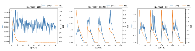
Figure 3: Plots of $||\Delta\theta||^{2}$ and train nll during training of l2e,csgmcmc, de on CIFAR-10. Unlike other methods, l2e actively updates $\theta$ in the local minima while maintaining training nll as nearly constant.

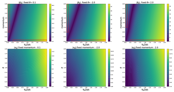
Figure 4: Countour plots of absolute value of outputs of $\beta_{\phi}$(top) and $\alpha_{\phi}$(bottom) on the grid. $\beta_{\phi}$ produces large magnitude of output when $\nabla_{\theta}\tilde{U}(\theta)$ is high. When $\nabla_{\theta}\tilde{U}(\theta)$ gets smaller, the overall magnitude decreases as expected, but even when $\nabla_{\theta}\tilde{U}(\theta)$ is nearly zero, $\beta_{\phi}$ can still allow the sampler to move around posterior distribution when integrated with high momentum value. The regions marked with red dashed boxes can be beneficial for exploration in high density regions. $\alpha_{\phi}$ is proportional to $\nabla_{\theta}\tilde{U}(\theta)$ in general, which helps the sampler fastly converge to the high density region.

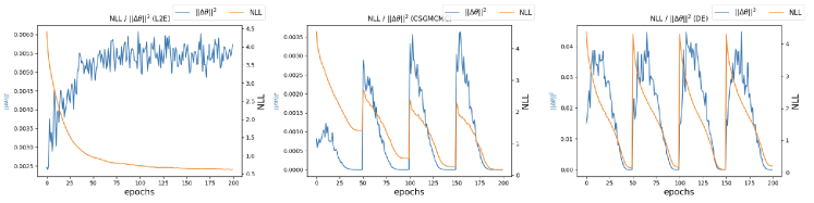
Figure 5: Plots of $||\Delta\theta||^{2}$ and train nll during training of l2e,csgmcmc, de on CIFAR-100.

In Figures 3 and 5, we find that l2e updates $\theta$ with a larger magnitude in local minima than in the early stages of training. This tendency is different from other gradient-based optimizer or mcmc methods where the amount of update is relatively small at local minima. Additionally, we notice that L2E actively updates $\theta$ at minima while maintaining loss as nearly constant. This trend is consistently observed in both CIFAR-10 and CIFAR-100, implying that l2e learns some common knowledge of posterior information across tasks for efficient exploration in low loss regions. Various experimental results (e.g., see Figure 2(b)) support that l2e is good at capturing multi-modalities of bnns posterior with a single trajectory. Since l2e produces significant amount of updates at local minima without increasing the loss, we can say that our parameterized gradients learned the general knowledge to explore high density regions among different modes.

In Figure 4, we plot absolute value of outputs of $\alpha_{\phi}$ and $\beta_{\phi}$ on the regular input grid. Since $\alpha_{\phi}$ and $\beta_{\phi}$ take $\theta,r,\nabla_{\theta}\tilde{U}(\theta)$ and running average of $\nabla_{\theta}\tilde{U}(\theta)$ as inputs, analyzing the function itself is a complex problem. Therefore, to simplify the analysis, we follow the approach of Gong et al. (2018), where we fix other inputs except for the statistics we are interested in. For $\beta_{\phi}$, we choose three different fixed values of $\theta$ and plot the results, while for $\alpha_{\phi}$, we fix the momentum. We assume that there is no running average of $\nabla_{\theta}\tilde{U}(\theta)$ so that running average term is fixed to $\nabla_{\theta}\tilde{U}(\theta)$.

Since the value of $\theta$ itself does not encode the information about the posterior landscape, there is no clear distinction among contour plots in top row with different $\theta$ values. In general, the scale of outputs of $\alpha_{\phi}$ and $\beta_{\phi}$ is proportional to $\nabla_{\theta}\tilde{U}(\theta)$ which is desirable for fast convergence to high density regions of posterior distribution. For $\beta_{\phi}$, when $\nabla_{\theta}\tilde{U}(\theta)$ gets smaller, the overall magnitude of output decreases as expected, but even when $\nabla_{\theta}\tilde{U}(\theta)$ is nearly zero, $\beta_{\phi}$ can still make large magnitude of update of $\theta$ when integrated with high momentum value. Also, when momentum is nearly zero, it still allows sampler to explore posterior distribution when $\nabla_{\theta}\tilde{U}(\theta)$ is far from zero. This complementary relationship between two statistics is strength of l2e that the movement of sampler is not solely depend on a single statistic so that it can exploit more complex information about loss geometry unlike standard SGHMC. $\alpha_{\phi}$ produces an output proportional to the scale of the gradient regardless of the momentum values. This implies that $\alpha_{\phi}$ helps the acceleration of sampler in low-density regions as it is added to the energy gradient in Equation 11.

One limitation of our analysis is that we focus on analyzing the magnitude of the function output rather than its direction. Although the magnitude of $\alpha_{\phi}$ and $\beta_{\phi}$ are closely connected to the exploration property, delving deeper into how L2E traverses complex and multi-modal bnns posterior landscape would be an interesting direction of future research.

Appendix B Bayesian Model Average(BMA) vs Cross-Entropy(CE) meta-loss

In this section, we will explain why bma meta-loss enhances the exploration of the sampler, by comparing it with CE meta-loss. Average CE loss of individual models along the optimizer’s trajectory on meta-training tasks has been used as a meta-objective to train learned optimizers (Andrychowicz et al., 2016; Metz et al., 2019, 2022b) on classification tasks. Two different objectives have following forms:

$$L^{\text{CE}}(\phi)=-\frac{1}{K}\sum_{k=1}^{K}\log p(y_{*}\,|\,x_{*},\theta_{k}(\phi))$$ (12)

$$L^{\text{\lx@glossaries@gls@link{acronym}{bma}{\leavevmode{bma}}}}(\phi)=-\log\frac{1}{K}\sum_{k=1}^{K}p(y_{*}\,|\,x_{*},\theta_{k}(\phi))$$

where $(x_{*},y_{*})$ is a validation data point. While bma meta-loss is similar to CE meta-loss, bma meta-loss differs significantly from CE meta-loss. bma meta-loss is Monte Carlo approximation of the posterior predictive distribution for validation data points. Actually, we gather models along the sampler’s trajectory and minimize CE-loss of the average probability of collected models. bma meta-loss not only encourages the sampler to minimize the average CE-loss of individual models but also promotes increased functional diversity among collected models. According to Wood et al. (2023, Equation 7), this loss of the ensemble model is decomposed as “ensemble loss = average individual loss - ambiguity”. Ambiguity refers to the difference among the ensemble models and individual models, and the larger it is, the more bma meta-loss decreases. In Figure 6, we observe that l2e trained with bma meta-loss exhibits a much greater loss barrier between collected parameters than l2e trained with CE meta-loss, indicating the higher exploration and larger functional diversity among samples. Also, our extensive downstream experiments and visualization demonstrates that L2E with bma meta-loss actually increases functional diversity among collected models.

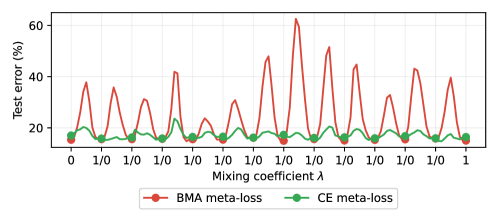
Figure 6: Ablation study of BMA vs CE meta-loss on CIFAR-10.

Appendix C l2e on Text Dataset

In order to check whether l2e can adapt well to the other modalities (e.g. text dataset), we additionally conduct text classification on IMDB dataset with CNN-LSTM architecture following Wenzel et al. (2020) and Izmailov et al. (2021b).

For hmc, we use checkpoints of 1200 samples from Izmailov et al. (2021b). For other MCMC methods, we collect 50 samples with 50 epochs of thinning interval with 100 burnin epochs. Appendix D demonstrates that l2e shows competitive performance on the text dataset, meaning that l2e can still work well on unseen modalities. This transfer of knowledge from image datasets to text dataset supports that the generalization capacity of l2e is strong compared to Gong et al. (2018), which is only proven to generalize well to similar datasets with meta-training dataset.

Appendix D Results on alternative parameterization

Although parameterizing $\nabla g(\theta,r)$ allows learned sampler to be expressive and efficient, we should make assumptions on the underlying $g(\theta,r)$. To avoid introducing additional assumptions, we propose another version of l2e that directly parameterizes kinetic energy function $g(\theta,r)$ rather than its gradients and evaluate whether it can achieve comparable performance comparable to l2e. Specifically, we fix $p(r|\theta)$ as normal distribution and parameterize its mean with $f_{\phi}(\theta)$ that takes $\theta,\nabla_{\theta}\tilde{U}(\theta)$ as inputs. This approach eliminates the need for assumptions regarding the existence and integrability of unnormalized probability density function. Since we set $p(r|\theta)\sim\mathcal{N}(f_{\phi}(\theta),I)$, kinetic energy function of $p(r|\theta)$ is $g(\theta,r)=(r-f_{\phi}(\theta))^{T}(r-f_{\phi}(\theta))$. Therefore, we can get $\nabla_{\theta}g(\theta,r)=f_{\phi}(\theta)\nabla_{\theta}f_{\phi}(\theta)$ and $\nabla_{r}g(\theta,r)=r-f_{\phi}(\theta)$. Then, update rule for this parameterization is as follows

$$r_{t+1}=r_{t}-\epsilon_{t}(\nabla_{\theta}\tilde{U}(\theta_{t})+f_{\phi}(\theta)\nabla_{\theta}f_{\phi}(\theta)+\alpha(r_{t}-f_{\phi}(\theta))+\xi_{t}$$ (13)

$$\theta_{t+1}=\theta_{t}+\epsilon_{t}(r_{t}-f_{\phi}(\theta))$$

where $\xi_{t}\sim{\mathcal{N}}(0,2\epsilon_{t}\alpha)$. We will refer to this version of sampler as Kinetic-l2e. In Appendix D, Kinetic-l2e shows comparable performance to l2e across all image classification experiments. Also, Figure 7 demonstrates the exploration capacity of Kinetc-l2e. These results indicate that both versions can achieve similar performance in terms of predictive accuracy and exploration.

Both versions of l2e have their own strength and weakness. l2e requires assumptions on the underlying kinetic energy function to ensure the convergence guarantee by Ma et al. (2015), but it is computationally efficient and can model complex functions. Kinetic-l2e guarantee the convergence without additional assumptions on $g(\theta,r)$, but requires additional gradient computations and conditional distribution $p(r|\theta)$ is restricted to specific distribution which can possibly harm the flexibility of the sampler. We recommend to consider these trade-offs for further applications.

Table 5: Results of kinetic energy parameterization of l2e.

Dataset	l2e	ACC $\uparrow$	NLL $\downarrow$	ECE $\downarrow$	KLD $\uparrow$
fashion-MNIST	Kinetic l2e	0.9175	0.2425	0.0104	0.1334
	l2e	0.9166	0.2408	0.0078	0.0507
CIFAR-10	Kinetic l2e	0.9131	0.2867	0.0527	0.4152
	l2e	0.9123	0.2909	0.0563	0.4344
CIFAR-100	Kinetic l2e	0.7013	1.114	0.1212	1.735
	l2e	0.6999	1.131	0.1403	1.749
Tiny-ImageNet	Kinetic l2e	0.5561	1.966	0.1731	1.907
	l2e	0.5583	1.846	0.1423	0.9139

Table 6: Results on IMDB classification task, following the experimental setup of Izmailov et al. (2021b)

Method	ACC $\uparrow$	NLL $\downarrow$
de	0.867$\scriptstyle{\pm 0.000}$	0.386$\scriptstyle{\pm 0.000}$
csgmcmc	0.848$\scriptstyle{\pm 0.007}$	0.401$\scriptstyle{\pm 0.032}$
hmc	0.868$\scriptstyle{\pm 0.000}$	0.308$\scriptstyle{\pm 0.000}$
Meta-sgmcmc	0.820$\scriptstyle{\pm 0.003}$	0.401$\scriptstyle{\pm 0.001}$
l2e	0.873$\scriptstyle{\pm 0.001}$	0.301$\scriptstyle{\pm 0.001}$

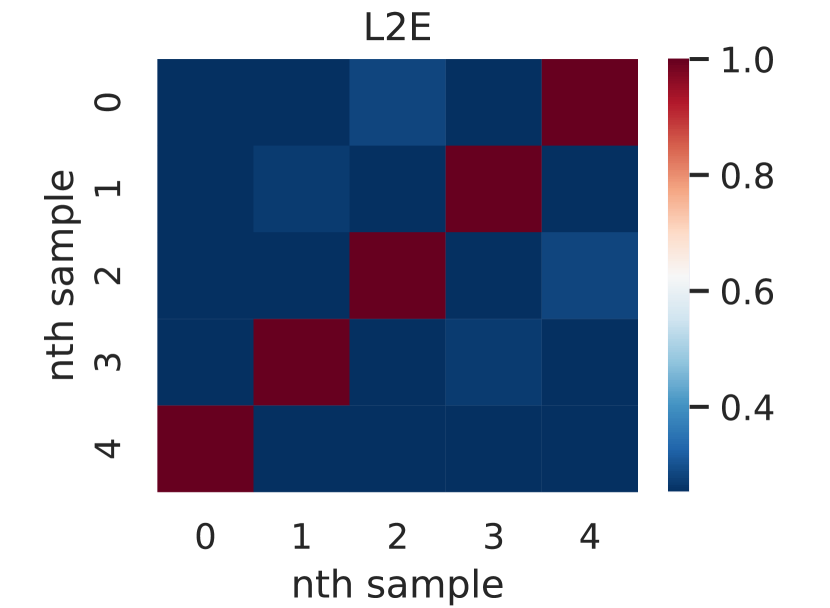
(a) Cosine similarity between weights.

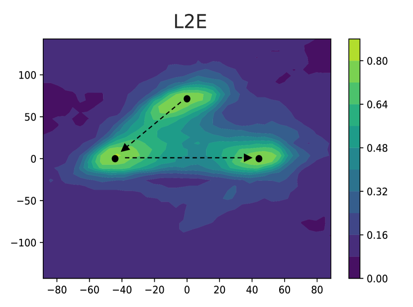
(b) Test error ($\%$) around the samples.

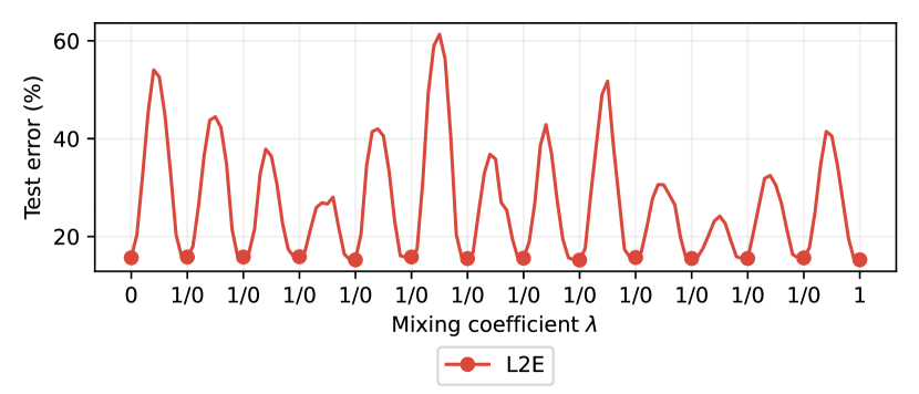
(c) Test error ($\%$) along linear path

Figure 7: Figures show multi-modality of l2e with parameterization of momentum distribution. (a) shows cosine similarity between weights. (b) is loss surface as a function of model parameters in a 2-dimensional subspace spanned by solutions of each method. Colors represent the level of test error. (c) shows test error ($\%$) along linear path between a pair of parameters.

Appendix E Comparision with Gong et al. (2018)

In Table 7, we demonstrate the difference between Meta-sgmcmc (Gong et al., 2018) and l2e. Meta-sgmcmc aims to build a sampler through meta-learning that rapidly converges to the target distribution and performs accurate simulation. This goal aligns with the objectives of all sgmcmc methods. However, our approach is specifically designed with the more concrete purpose of effectively simulating multi-modal DNN posterior distribution and also generalizing to unseen problems. We compare l2e to Meta-sgmcmc in various aspects in the following subsections.

Table 7: Comparison between Gong et al. (2018) and L2E

	Gong et al. (2018)	l2e
Purpose of meta-learning	Fast convergence, low bias	Efficient exploration of multi-modal bnns posterior
Learning target	Diffusion and curl matrix	Gradient of kinetic energy
Meta-training task	Single-task	Multi-task
Meta-objective	$\textrm{KL}(q_{t}|\pi)$	$-\log\frac{1}{K}\sum_{k=1}^{K}p(y_{*}\,|\,x_{*},\theta_{k}(\phi))$
Meta-gradient estimation	tbptt (Werbos, 1990)	es (Salimans et al., 2017)
Generalizes to	unseen classes in the same dataset	completely different datasets
Scales to	small scale architecture	large scale architecture

Table 8: Experiments on CIFAR-10 following experiments in Gong et al. (2018). Without having seen CIFAR-10 dataset during meta training, l2e outperforms reported performance of Meta-sgmcmc while using significantly less computational cost than Meta-sgmcmc

. Methods NT ACC NT+AF ACC NT+Data ACC NT NLL/100 NT+AF NLL/100 NT+Data NLL/100 Meta-sgmcmc 78.12$\scriptstyle{\pm 0.035}$ 74.41$\scriptstyle{\pm 0.11}$ 89.97$\scriptstyle{\pm 0.04}$ 68.88$\scriptstyle{\pm 0.15}$ 79.55$\scriptstyle{\pm 0.057}$ 15.66$\scriptstyle{\pm 0.28}$ l2e 79.21$\scriptstyle{\pm 0.203}$ 75.91$\scriptstyle{\pm 0.200}$ 92.49$\scriptstyle{\pm 0.234}$ 63.23$\scriptstyle{\pm 0.46}$ 72.11$\scriptstyle{\pm 0.22}$ 11.82$\scriptstyle{\pm 0.81}$

Table 9: Experiments on MNIST following experiments in Gong et al. (2018)

. Methods NT ACC NT+AF ACC NT+Data ACC NT NLL/100 NT+AF NLL/100 NT+Data NLL/100 Meta-sgmcmc 98.36$\scriptstyle{\pm 0.02}$ 97.72$\scriptstyle{\pm 0.02}$ 98.62$\scriptstyle{\pm 0.02}$ 640$\scriptstyle{\pm 6.25}$ 875$\scriptstyle{\pm 3.19}$ 230$\scriptstyle{\pm 3.23}$ l2e 98.39$\scriptstyle{\pm 0.05}$ 98.07$\scriptstyle{\pm 0.08}$ - 558$\scriptstyle{\pm 3.19}$ 679$\scriptstyle{\pm 6.65}$ -

E.1 Difference in parameterization of meta models

The update rule for $z=(\theta,r)\in\mathbb{R}^{2d}$ presented in Gong et al. (2018) is as following.

$$r_{t+1}=(1-\epsilon_{t}D_{f}(z_{t}))r_{t}-\epsilon_{t}Q_{f}(z_{t})\nabla_{\theta}\tilde{U}(\theta_{t})+\epsilon_{t}\Gamma_{r}(z_{t})+\xi_{t}$$ (14)

$$\theta_{t+1}=\theta_{t}+\epsilon_{t}Q_{f}(z_{t})r_{t}+\epsilon_{t}\Gamma_{\theta}(z_{t})$$

$$\xi_{t}\sim{\mathcal{N}}(0,2\epsilon_{t}D_{f}(z_{t})),\quad\Gamma_{i}(z):=\sum_{j=1}^{2d}\frac{\partial}{\partial z_{j}}(D_{ij}(z)+Q_{ij}(z))$$

In our main text, we point out that parameterizing $D_{f}$ and $Q_{f}$ makes additional computational burden. Additionally, since $D_{f}$ and $Q_{f}$ mainly function as multipliers for gradient and momentum, learning them may not be as effective as it should be for effective exploration in low energy regions. In low energy regions where the norm of gradient and momentum are extremely small, it is difficult to make reasonable amount of update of $\theta$ for exploration by multiplying $Q_{f}$ to momentum and gradient. Also, $Q_{f}$ should be clipped by some threshold for practical issue. By contrast, In the update rule of l2e (6), $\alpha_{\phi},\beta_{\phi}$ are added to the gradient, which is more suitable for controlling the magnitude and direction of update in low energy regions. Also, ablation study in Table 11 shows the inferior performance of learning $D_{f}$ and $Q_{f}$ in terms of classification accuracy and predictive diversity in our setting. Therefore, we choose to learning kinetic energy gradient is better than learning $D_{f}$ and $Q_{f}$, as it avoids additional computation and allows the sampler to mix better especially around the low energy region.

E.2 Difference in meta-training procedure

There are significant differences between two methods in meta-training pipeline. Firstly, the most notable distinction is that Meta-sgmcmc learns with only one task, requiring the training of a new learner for each problem. This poses an issue as a single learner may not generally apply well to various problems. In contrast, our approach involves sampling from a task set composed of diverse datasets and architectures for training. Another crucial difference is the choice of estimator for the meta-objective gradients. Gong et al. (2018) employs Truncated BackPropagation Through Time (tbptt) which truncates computational graphs of a long inner-loop to estimate the meta gradient. While this approach can save computational cost by avoiding backpropagation through long computational graph, it results in a biased estimator of meta-gradient. To address these issues, we utilize es to compute unbiased estimator of meta-gradient efficiently.

E.3 Experimental results

In order to compare l2e with Meta-sgmcmc, we exactly replicate the experimental setup of MNIST and CIFAR-10 experiments in Gong et al. (2018) and evaluate performance of l2e. These experiments evaluate how well each method generalizes to unseen Neural Network architecture (NT), activation function (AF) and dataset (Data) which were unseen during the meta-learning process. For the experimental details, please refer to the experiments section of Gong et al. (2018). We use same scale of metrics in Gong et al. (2018) for conveniently comparing two methods. We report Accuracy (acc) and nll on test dataset. Since l2e used MNIST dataset during meta-train, we do not evaluate Dataset generalization experiments on MNIST. Meta-sgmcmc used 20 parallel chains with 100 epochs for MNIST and 200 epochs for CIFAR-10. We use single chain with 100 burn-in epochs for both experiments, and use 10 thinning epochs for collecting 20 samples.

In LABEL:metavl2ecifar and LABEL:metavl2emnist, we confirm that l2e outperforms Meta-sgmcmc for all generalization types in terms of acc and nll despite using significantly less computational cost. Notably, in CIFAR-10 experiment, despite l2e was not trained on the CIFAR-10 during meta-learning, l2e significantly outperforms Meta-SGMCMC with a wide margin indicating that our approach better generalizes to unseen datasets compared to Meta-sgmcmc.

Appendix F Discussion on meta-training objectives

Previous studies have proposed various meta-objectives to achieve goals similar to ours. Gong et al. (2018) minimizes the $\textrm{KL}(q_{t}|\pi)$, where $\pi$ is target distribution and $q_{t}$ is the marginal distribution of $\theta$ at time $t$ for good mixing. On the other hand, Levy et al. (2017) employs meta-objective maximizing the jump distances between samples in weight space and simultaneously minimizing the energy in order to make sampler rapidly explore between modes. However, explicitly maximizing the jump distances in weight space can be easily cheated, as the distances between weights does not necessarily lead to the difference in the functions, resulting in trivial sampler with which achieving the balance between convergence and exploration is hard. Also, minimizing the divergence with target distribution seems sensible, but due to intractable $q_{t}$, computing the gradient of $q_{t}$ should resort to gradient estimator. Gong et al. (2018) used stein-gradient estimator, which requires multiple independent chains so it harms scalability. Also, this objective does not lead the learned sampler to explore multi-modal distribution. Gong et al. (2018, Figure 3) shows that the learned sampler quickly converges to low energy region, but learned friction term $D_{f}$ restricts the amount of update in low energy region, limiting the exploration behaviour. Among choices, we find out that BMA meta-loss is a simple yet effective meta-objective that naturally encodes exploration-exploitation balance without numerical instability and exhaustive hyperparameter tuning.

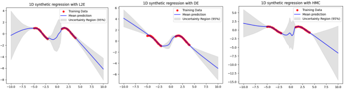
Figure 8: 1-D synthetic regression of l2e, de, hmc. See Appendix G for details and discussion.

Appendix G 1-D synthetic regression

We conduct 1-D synthetic regression task to visually check whether l2e can capture the epistemic uncertainty. For the training data, we generate 1000 data points from underlying true function $y=\sin(x)$, within the interval $[-5,1]$ and $[1,4]$. We use de and hmc as baselines. We collect 50 parameters for each methods and plot the mean prediction and $95\%$ confidence interval of the prediction. For l2e, we do not fine-tune the learned sampler used in the main experiments. We use thinning interval of 50 training steps and 1000 burn-in steps for l2e, 300 training steps for each single solution of de and 1000 burn-in steps and 100 leap-frog steps for hmc. We use 2 layers MLP with 100 hidden units and ReLU activation to estimate the function.

Effective method for capturing epistemic uncertainty should make confident predictions for the training data and should be uncertain on ood data points. Figure 8 shows that l2e better captures ’in-between’ uncertainty than de. l2e generally produces diverse predictions for out-of-distribution data points, especially for the input space between two clusters of training data while de shows relatively confident prediction in that region. hmc is known for the golden standard for posterior inference in Bayesian method. Our experimental result aligns with this common knowledge since hmc is the best in terms of capturing epistemic uncertainty among three methods especially in areas out of the range of training points. While our approach falls short of hmc, it demonstrates better uncertainty estimation than that of de and shows similar predictive uncertainty with hmc between two training points cluster. These experimental results align with the ood detection experiments and convergence diagnostics presented in our main text, indicating l2e performs effective posterior inference. It is important to note that even without meta-training on the regression datasets, l2e can adapt well to the regression problem.

Appendix H Image classification with Data Augmentation

Since applying data augmentation violates Independently and Identically Distributed(IID) assumption of the dataset which is commonly assumed by Bayesian methods, this can lead to model misspecification (Wenzel et al., 2020; Kapoor et al., 2022) and under model misspecifcation, bayesian posterior may not be the optimal for the bma performance (Masegosa, 2020). Therefore, prior work such as Izmailov et al. (2021b) argued the incompatibility between Bayesian methods and data augmentation. However, data augmentation is an indispensable technique in modern machine learning so it is also interesting to see how l2e performs with data augmentation. We run the image classification experiments on CIFAR-10 and CIFAR-100 with random crop and horizontal flip for the data augmentation. Since using data augmentation introduces Cold Posterior Effect (Wenzel et al., 2020) for Bayesian methods such as csgmcmc and l2e, we additionally tune the temperature hyperparameter for these methods. We tune the temperature for each methods, using $T=0.0001$ in both experiments. Please refer to  Wenzel et al. (2020) for detailed analysis of Cold Posterior Effect. We collect 10 samples for all methods for these experiments.

In Table 10, when applying data augmentation, the performance gap between csgmcmc and l2e becomes far less stark than without data augmentation. Moreover, de outperforms other baselines with a large margin in CIFAR-10 and shows similar results with l2e in CIFAR-100 since l2e significantly outperforms other method without data augmentation. With data augmentation, it is not very surprising that de outperforms other Bayesian methods like l2e and csgmcmc in terms of predictive accuracy and calibration since they suffer from model misspecification and temperature tuning can partially handle this problem (Kapoor et al., 2022). Observing the high agreement between l2e and hmc in the function space suggests that l2e effectively approximates the predictive distribution of the target posterior distribution. However, when techniques that violate assumptions for model likelihood are applied, correctly simulating target distribution does not necessarily mean the superior performance than other methods. As a result, there may be a reduction or even a reversal in the performance gap compared to other methods. Nevertheless, l2e demonstrates comparable performance to DE with less compute on datasets like CIFAR-100. Also, l2e shows slightly better performance than Bayesian method,csgmcmc in CIFAR-10 and outperforms with a wide margin in CIFAR-100 experiment. When it comes to predictive diversity, l2e significantly outperforms baselines on both experiments. Although applying data augmentation introduces significant variations to the posterior landscape, we confirm that l2e still maintains the exploration property. To sum up, we argue that l2e is still practical method even with data augmentation since it shows competitive predictive performance and efficiently explores the posterior landscape.

Table 10: Results of image classification with data augmentation.

Dataset	Method	ACC $\uparrow$	NLL $\downarrow$	ECE $\downarrow$	KLD $\uparrow$
CIFAR-10	de	0.931$\scriptstyle{\pm 0.002}$	0.209$\scriptstyle{\pm 0.003}$	0.017$\scriptstyle{\pm 0.001}$	0.293$\scriptstyle{\pm 0.002}$
	csgmcmc	0.923$\scriptstyle{\pm 0.003}$	0.234$\scriptstyle{\pm 0.007}$	0.031$\scriptstyle{\pm 0.005}$	0.142$\scriptstyle{\pm 0.019}$
	l2e	0.926$\scriptstyle{\pm 0.001}$	0.235$\scriptstyle{\pm 0.002}$	0.037$\scriptstyle{\pm 0.001}$	0.391$\scriptstyle{\pm 0.005}$
CIFAR-100	de	0.708$\scriptstyle{\pm 0.001}$	1.048$\scriptstyle{\pm 0.001}$	0.092$\scriptstyle{\pm 0.001}$	0.765$\scriptstyle{\pm 0.003}$
	csgmcmc	0.683$\scriptstyle{\pm 0.001}$	1.114$\scriptstyle{\pm 0.005}$	0.013$\scriptstyle{\pm 0.001}$	0.319$\scriptstyle{\pm 0.008}$
	l2e	0.705$\scriptstyle{\pm 0.003}$	1.066$\scriptstyle{\pm 0.001}$	0.095$\scriptstyle{\pm 0.003}$	0.996$\scriptstyle{\pm 0.017}$

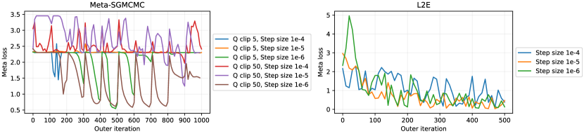
Figure 9: Meta loss at each outer iteration during the meta training process. For Meta-sgmcmc, it is evident that the meta loss is highly unstable depending on hyperparameters such as Q clip and step size. Conversely, with l2e, it can be observed that the meta loss converges stably even with varying step size values.

Appendix I Details for meta-training

For meta-training, we construct our experiment code based on JAX learned-optimization package (Metz et al., 2022a). Also, we build our own meta-loss and l2e with specific input features and design choice. Therefore, we construct our own meta-learning task distribution that l2e can efficiently learn knowledge for better generalization for large-scale image classification task.

I.1 Input features

We use the following input features for l2e:

• raw gradient values

• raw parameter values

• raw momentum values

• running average of gradient values

Running average feature is expanded for multiple time scale in that we use multiple momentum-decay values for averaging. We use 0.1, 0.5, 0.9, 0.99, 0.999 and 0.9999 for momentum decay so that running average feature is expanded into 6-dimensions. Therefore, we have total 9-dimensional input features for each dimension of parameter and momentum. Input features are normalized so that $l2$ norm with respect to input features of different dimensions become 1. $\alpha_{\phi}$ and $\beta_{\phi}$ share weights of neural network except for the last layer of mlp, so that we can get two quantities with single forward pass. This weight sharing method is employed in Levy et al. (2017) or other recent literature in learned optimization like in Metz et al. (2022b) and Metz et al. (2019).

1:  Input: Meta parameter $\phi$, inner iterations $N_{\text{inner}}$, initial parameter $\theta_{0}$, step size $\varepsilon$, burn-in steps $B$, thinning interval $T$.

2:  Output: Loss $L(\phi)$

3:  Initialize $\Theta=\varnothing$ and $r_{0}\sim{\mathcal{N}}(0,I_{d})$.

4:  for $i=1,\dots,N_{\text{inner}}$ do

5:     $r_{t+1}=r_{t}-\epsilon_{t}(\nabla\tilde{U}(\theta_{t})+\alpha_{\phi}+c\beta_{\phi})+\xi_{t}$ where $\xi_{t}\sim{\mathcal{N}}(0,2c)$.

6:     $\theta_{t+1}=\theta_{t}+\epsilon_{t}\beta_{\phi}$

7:     if $i>B\;\&\mod(i,T)=0$ then

8:        $\Theta\leftarrow\Theta\cup\{\theta_{i}\}$

9:     end if

10:  end for

11:  $L(\phi)\leftarrow-\log\frac{1}{|\Theta|}\sum_{\theta\in\Theta}p(y^{*}|x^{*},\theta)$

Algorithm 2 InnerLoop

I.2 Task distribution

Dataset

We use MNIST, Fashion-MNIST, EMNIST and MedMNIST for meta training. We do not use resized version of dataset for meta training. For MedMNIST, we use the BloodMNIST in the official website.

Neural network architecture

At each outer iteration, we randomly sample one configuration of neural network architecture which is constructed by the possible choice below. We use the following options for neural network architecture variation:

• Size of the convolution output channel : $\{4,8,16\}$

• Number of convolution layers: $\{1,2,3,4,5\}$

• Presence of the residual connection: boolean

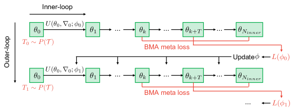
Figure 10: Meta learning procedure of l2e.

I.3 meta-training procedure

General hyperparameter

For meta-training, we fix the length of the inner loop for all tasks at 3000 iterations. We determine this by monitoring the meta-objective during training and set sufficient length of inner loop for l2e to enter to high-density region regardless of tasks. This setting can vary when task distribution is changed. To compute the meta-objective, we collect 10 inner-parameters with a thinning interval of 50 during the last 500 iterations of the inner-loop. We find out that this thinning interval and the number of collected inner parameters do not have a significant impact on the model performance. Also, we use 1000 iterations of outer-loop for training meta-parameter since meta-loss converges after 1000 outer iterations.

Outer optimization

For training meta-parameter, we use Adam with learning rate 0.01 and $\beta_{1}=0.9,\beta_{2}=0.99$. We apply gradient clipping to the gradient of meta-objective to prevent unstable training due to the different gradient scale among tasks.

I.4 Meta-sgmcmc meta-training procedure

General setup

For meta-training, we use the same task distribution as l2e do to fairly compare generalizability of two methods. We use 1-layer MLP with 10 hidden units for $Q_{f}$ and $D_{f}$. Since output of $D_{f}$ restricted to positive value, we take absolute value of output of $D_{f}$. We modify some original input preprocessing method different from Gong et al. (2018). Firstly, they heuristically find some good values to scale the input for $Q_{f}$ and $D_{f}$. This does not work in multi-task training as hyperparameter tuning is task specific, we scale the norm of input of neural networks as l2e do.

For meta-training, we use tbptt as the gradient estimator for meta-parameter. We use total 5000 inner-steps as a single problem and use 50 steps for truncation length. After running 5000 steps for one task, we freshly sample the task for training meta-sgmcmc, which is completely different from Gong et al. (2018) and similar to l2e. Since Gong et al. (2018) used 15 steps for truncation length, we find out that lengthen the truncation length can improve the performance. Also, we tune the band width length and use 100 for stein gradient estimator.

hyperparameters

For step size, we use 1e-06 since larger step size does not work in our task distribution for Meta-sgmcmc. Please refer to Figure 9 for sensitivity of Meta-sgmcmc compared to l2e. We us 5 for clipping values of $Q_{f}$ and 100 for $D_{f}$. For implementing meta-objective, we follow the official implementation of the meta-objective except for number of chains due to memory consumption. We use 2 chains for running Meta-sgmcmc on our task-distribution.

Outer optimization

For training meta-parameter, we use Adam with learning rate 0.0003 and $\beta_{1}=0.9,\beta_{2}=0.99$. We apply gradient clipping to the gradient of meta-objective to prevent unstable training due to the different gradient scale among tasks. We train meta-models for 1000 outer-iteration while saving the meta-models for every 100 outer iterations. Since training Meta-sgmcmc is significantly unstable as shown in Figure 9, we choose the best sampler by evaluating every saved meta-models for fashion-MNIST and CIFAR-10 tasks.

Appendix J Ablation studies

Table 11: Results of ablation studies. We use 10 samples for ablation studies. l2e shows the best performance among other choices. Notable result is that the performance gap between small l2e gets larger as the size of task gets bigger. This implies that task distribution of meta-training plays important role for generalization capability. Precond l2e shows worse performance in general and diverge in Tiny-ImageNet task. This parameterization shows worse performance and less generalizability than kinetic gradient parameterization.

Dataset	l2e	ACC $\uparrow$	NLL $\downarrow$	ECE $\downarrow$	KLD $\uparrow$
fashion-MNIST	Small l2e	0.9158	0.2520	0.0120	0.0797
	Precond l2e	0.8801	0.3461	0.0382	0.2597
	l2e	0.9166	0.2408	0.0078	0.0507
CIFAR-10	Small l2e	0.8952	0.3465	0.0610	0.5008
	Precond l2e	0.7503	0.7950	0.1349	0.4126
	l2e	0.9009	0.3231	0.0480	0.6263
CIFAR-100	Small l2e	0.6536	1.3067	0.1237	1.4391
	Precond l2e	0.3397	2.6761	0.1508	0.7449
	l2e	0.6702	1.2345	0.1224	1.2632
Tiny-ImageNet	Small l2e	0.4759	2.318	0.0672	2.8437
	Precond l2e	-	-	-	-
	l2e	0.5287	1.979	0.1478	0.8124

In Table 11, we demonstrate the results from our ablations studies. We evaluate how the size of task set can affect the generalization performance of l2e and the parameterization choice can make impact on the performance. We use following two variants of l2e

• Small l2e: meta-trained on only one dataset, using small architectures. In detail, this model only use Fashion-MNIST dataset and channel sizes of 4 and depths of 1 and 2 are possible choices of random configuration.

• Precond l2e: Parameterization of l2e changes from designing kinetic energy gradient to preconditioner.

Firstly, we confirm that l2e trained with larger task distribution shows better generalization performance. Although small l2e shows decent performance on Fashion-MNIST and CIFAR-10, it shows significant drop of performance in Tiny-ImageNet and CIFAR-100. This implies that further scaling of task distribution can lead l2e to show better performance in diverse unseen tasks. Also, we compare the method parameterizing $D(z),Q(z)$ with neural networks as in Gong et al. (2018). This shows that our parameterization is significantly better than designing preconditioner. Since preconditioner matrix can only work as multiplier of learning rate or noise scale, it has limitation for its expressivity which shows limitation in bnns.

Appendix K Experimental Details

We use JAX library to conduct our experiments. We use NVIDIA RTX-3090 GPU with 24GB VRAM and NVIDIA RTX A6000 with 48GB for all experiments. We implement meta-training algorithm based on the learned-optimization package (Metz et al., 2022a) with some modifications.

K.1 Real-world image classification

Dataset

We use tensorflow dataset for fashion-MNIST, CIFAR-10 and CIFAR-100. We utilize Tiny-ImageNet with image size of 64x64.

Architecture

We use 1 layer convolution neural network on fashion-MNIST and ResNet56-FRN with Swish activation on Tiny-ImageNet.

Hyperparameter

Table 12: Hyperparameters for de.

Method	fashion-MNIST	CIFAR-10	CIFAR-100	Tiny-ImageNet
Optimizer	SGDM	SGDM	SGDM	SGDM
Num models	100	100	100	10
Total epochs	10000	10000	10000	2000
Initial learning rate	$0.1$	$0.1$	$0.1$	$0.1$
Learning rate schedule	Cosine decay	Cosine decay	Cosine decay	Cosine decay
momentum decay	0.5	0.1	0.05	0.3
Weight decay	$5\times 10^{-4}$	$1\times 10^{-3}$	$5\times 10^{-4}$	$5\times 10^{-4}$
Batch size	128	128	128	128

Table 13: Hyperparameters for csgmcmc.

Method	fashion-MNIST	CIFAR-10	CIFAR-100	Tiny-ImageNet
Num burn in epochs	100	100	100	100
Num models	100	100	100	10
Total epochs	5100	5100	5100	1100
Thinning interval	50	50	50	50
exploration ratio	0.8	0.94	0.94	0.8
Step size	$2\times 10^{-6}$	$1\times 10^{-6}$	$1\times 10^{-6}$	$1\times 10^{-6}$
Step size schedule	Cosine	Cosine	Cosine	Cosine
Momentum decay	0.5	0.01	0.01	0.05
Weight decay	$5\times 10^{-4}$	$1\times 10^{-3}$	$1\times 10^{-3}$	$5\times 10^{-4}$
Batch size	128	128	128	128

Table 14: Hyperparameters for l2e.

Method	fashion-MNIST	CIFAR-10	CIFAR-100	Tiny-ImageNet
Num burn in epochs	100	100	100	100
Num models	100	100	100	10
Total epochs	5100	5100	5100	1100
Thinning interval	50	50	50	20
Step size schedule	Constant	Constant	Constant	Constant
Momentum decay	0.05	0.05	0.05	0.05
Weight decay	$5\times 10^{-4}$	$5\times 10^{-4}$	$5\times 10^{-4}$	$5\times 10^{-4}$
Batch size	128	128	128	128
Step size	$2\times 10^{-5}$	$2\times 10^{-5}$	$1\times 10^{-4}$	$2\times 10^{-4}$

We report hyperparameters for each methods in Table 12, Table 13 and Table 14. We tune the hyperparameters of methods using bma nll as criterion with number of 10 samples. For all methods including l2e, we tune learning rate(step size), weight decay(prior variance) and momentum decay term. We use zero-mean gaussian as prior distribution for sgmcmc methods, so that prior variance is equal to half of the inverse of weight decay. For momentum decay, we grid search over $\alpha\in\{0.01,0.05,0.1,0.3,0.5\}$. For weight decay, we also search over $\lambda\in\{1e-04,5e-04,1e-03\}$ to find best configuration. For step size, except for l2e, we search over $\epsilon\in\{2e-7,4e-7,1e-6,2e-6,4e-6,1e-5\}$. For l2e, due to scale of output of meta-learner, we additionaly search over bigger step size including $2e-5$, $1e-4$, $2e-4$.

Baselines

We use the following as baseline methods

• Deep ensembles (Lakshminarayanan et al., 2017) : This method collects parameters trained from multiple different initialization for ensembling. de is often compared with Bayesian methods in recent bnns literature like in Izmailov et al. (2021b) in that de induce similar function to hmc which is golden standard in bnns with bma.

• Cyclical Stochastic Gradient MCMC (Zhang et al., 2020): Zhang et al. (2020) introduced cyclic learning rate schedule to sgmcmc for improving exploration of sampler. csgmcmc usually shows descent predictive performance comparing to other existing sgmcmc methods in large-scale experiments.

• Meta-sgmcmc (Gong et al., 2018): Gong et al. (2018) proposed to meta-learn curl and diffusion matrix of sgmcmc to build sampler that can fastly converge to target distribution with small bias.

Metrics

Let $p(y|x,\theta)\in[0,1]^{K}$ be a predicted probabilities for a given input $x$ with label $y$ and $\theta$ is model parameter. $p^{(k)}$ denotes the $k$th element of the probability vector. We have the following common metrics on the dataset ${\mathcal{D}}$ consists of inputs $x$ and labels $y$:

• Accuracy (ACC):

  $$\operatorname{ACC}({\mathcal{D}})=\mathbb{E}_{(x,y)\in{\mathcal{D}}}\left[I\left[y=\operatorname*{arg\,max}_{k}p^{(k)}(x)\right]\right].$$ (15)

• Negative log-likelihood (NLL):

  $$\operatorname{NLL}({\mathcal{D}})=\mathbb{E}_{(x,y)\in{\mathcal{D}}}\left[-\log{p^{(y)}(x)}\right].$$ (16)

• Expected calibration error (ECE): Actual implementation of Expected Calibration Error (ece) includes dividing predicted probabilities with their confidence. We use following implementation

  $$\operatorname{ECE}({\mathcal{D}},N_{\text{bin}})=\sum_{b=1}^{N_{\text{bin}}}\frac{n_{b}|\delta_{b}|}{n_{1}+\cdots+n_{N_{\text{bin}}}},$$ (17)

  where $N_{\text{bin}}$ is the number of bins, $n_{b}$ is the number of examples in the $b$th bin, and $\delta_{b}$ is the calibration error of the $b$th bin. We use $N_{\text{bin}}=15$ for computing ece.

• Pairwise Kullback-Leibler Divergence(KLD): Given set of ensemble members $\Theta=\{\theta_{i}\dots\theta_{M}\}$, we construct matrix $A$ using pair of ensemble members which have $A_{ij}=p(y|x,\theta_{i})\log\frac{p(y|x,\theta_{i})}{p(y|x,\theta_{j})}$ for a given input $x$ and $y$. We calculate the statistic as follows

  $$D_{\mathrm{KL}}({\mathcal{D}},M)=\mathbb{E}_{(x,y)\in{\mathcal{D}}}\left[{\frac{1}{M(M-1)}\sum_{i\neq j}A_{ij}}\right].$$ (18)

• Agreement: The Agreement is defined as the alignment between the top-1 predictions of the HMC and our own predictions. This metric is computed through the following formula:

  $$\operatorname{Agreement}({\mathcal{D}})=\mathbb{E}_{(x,y)\in{\mathcal{D}}}\left[I\left[\operatorname*{arg\,max}_{k}\hat{p}^{(k)}(x)=\operatorname*{arg\,max}_{k}p^{(k)}(x)\right]\right],$$ (19)

  where $I[\cdot]$ is indicator function and $\hat{p}$ is predictive distribution of HMC. It indicates how well a method is able to capture the top-1 predictions of HMC.

• Total Variation(Total Var): Total Variation quantifies the total variation distance between the predictive distribution of the HMC and our own predictions averaged over the data points. Specifically, it compares the predictive probabilities for each of the classes as follows

  $$\operatorname{TotalVar}({\mathcal{D}})=\mathbb{E}_{(x,y)\in{\mathcal{D}}}\left[\frac{1}{2}\sum_{k}\left|\hat{p}^{(k)}(x)-p^{(k)}(x)\right|\right].$$ (20)

K.2 Computational cost

Table 15: Wall clock time(sec) of sgmcmc methods per single epoch. Measured using NVIDIA RTX A6000.

Method	fashion-MNIST	CIFAR-10	CIFAR-100	Tiny-ImageNet
csgmcmc	0.20	1.79	1.81	41.12
Meta-sgmcmc	0.32	2.44	2.45	47.22
l2e	0.32	2.64	2.66	48.43

Table 15 shows the actual computational time for each methods. l2e does not incur significant computational overhead.

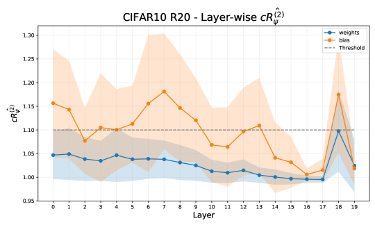
Figure 11: Layerwise convergence of weights and biases on CIFAR-10 ResNet experiment.

Appendix L Implementation of Convergence Diagnostics

For Effective Sample Size (ess), we use Tensorflow Probability (Lao et al., 2020) library for implementation. We use default parameter of the implementation. ess is then normalized to the time consumed for running one thinning interval, which is equivalent to 50 epochs. Since scale of ess is too large to report since dimension of neural network parameters are huge for our experiments, we divide it by $10^{-5}$ and report for convenience.

$\hat{R}$ (Gelman & Rubin, 1992) has been widely employed to measure the convergence of MCMC chain. However, in modern bnns, due to the multimodality in bnns posterior distribution, traditional $\hat{R}$ without further modification is meaningless in the parameter space(Sommer et al., 2024). Sommer et al. (2024) demonstrated that parameter space convergence should be measured both chain- and layer-wise to fix these issues. Basically, $c\hat{R_{\psi}^{(\kappa)}}$ diagnostic splits a single chain’s path into $\kappa$ sub chains for $\hat{R}$ calculation. Therefore, we report the proportion of parameters with $c\hat{R_{\psi}^{(\kappa)}}<1.1$ using code implementation of Sommer et al. (2024) for our main results. We set $\kappa=2$ considering the number of collected parameters in our experiments. Please refer to Sommer et al. (2024) for detailed description of this metric. In Figure 11, we also demonstrate layer-wise visualization of $c\hat{R_{\psi}^{(\kappa)}}$. For weights, l2e shows good convergence performance in terms of layer-wise $c\hat{R_{\psi}^{(\kappa)}}$ while convergence of biases is mixed across the layers. Considering that weights account for the majority of the parameters, we confirm that l2e shows strong convergence in terms of layer-wise $c\hat{R_{\psi}^{(\kappa)}}$.

Appendix M Limitation of l2e

While effective, l2e has some limitations that should be considered for applications. Firstly, l2e requires additional meta-training costs. In our experiment, meta-training takes approximately 6 hours on a single NVIDIA RTX A6000 GPU, but it possibly requires more computational cost for meta-training using larger tasks. While L2E demonstrates good performance across various data domains, in Table 11, we observe that the performance of l2e is influenced by the size of the meta-training distribution as the scale of the target problem increases. In other words, there is a possibility that we may need to meta-train L2E with larger datasets and architectures to apply L2E to very large models and datasets.

References

- Andrychowicz et al. (2016) Andrychowicz, M., Denil, M., Gomez, S., Hoffman, M. W., Pfau, D., Schaul, T., Shillingford, B., and De Freitas, N. Learning to learn by gradient descent by gradient descent. Advances in neural information processing systems, 29, 2016.
- Betancourt (2017) Betancourt, M. A conceptual introduction to hamiltonian monte carlo. arXiv preprint arXiv:1701.02434, 2017.
- Blei & McAuliffe (2017) Blei, D. M. an Kucukelbir, A. and McAuliffe, J. D. Variational inference: a review for statisticians. Journal of the American Statistical Association, 112(518):859–877, 2017.
- Chen et al. (2014) Chen, T., Fox, E., and Guestrin, C. Stochastic gradient hamiltonian monte carlo. In International conference on machine learning, pp. 1683–1691. PMLR, 2014.
- Cohen et al. (2017) Cohen, G., Afshar, S., Tapson, J., and Van Schaik, A. EMNIST: Extending MNIST to handwritten letters. In 2017 international joint conference on neural networks (IJCNN), pp. 2921–2926. IEEE, 2017.
- Fort et al. (2019) Fort, S., Hu, H., and Lakshminarayanan, B. Deep ensembles: A loss landscape perspective. arXiv preprint arXiv:1912.02757, 2019.
- Garipov et al. (2018) Garipov, T., Izmailov, P., Podoprikhin, D., Vetrov, D. P., and Wilson, A. G. Loss surfaces, mode connectivity, and fast ensembling of dnns. Advances in neural information processing systems, 31, 2018.
- Gelman & Rubin (1992) Gelman, A. and Rubin, D. B. Inference from iterative simulation using multiple sequences. Statistical science, 7(4):457–472, 1992.
- Girolami & Calderhead (2011) Girolami, M. and Calderhead, B. Riemann manifold langevin and hamiltonian monte carlo methods. Journal of the Royal Statistical Society Series B: Statistical Methodology, 73(2):123–214, 2011.
- Gong et al. (2018) Gong, W., Li, Y., and Hernández-Lobato, J. M. Meta-learning for stochastic gradient mcmc. In International Conference on Learning Representations, 2018.
- Goodfellow et al. (2014) Goodfellow, I. J., Vinyals, O., and Saxe, A. M. Qualitatively characterizing neural network optimization problems. arXiv preprint arXiv:1412.6544, 2014.
- Hendrycks & Dietterich (2019) Hendrycks, D. and Dietterich, T. Benchmarking neural network robustness to common corruptions and perturbations. arXiv preprint arXiv:1903.12261, 2019.
- Izmailov et al. (2021a) Izmailov, P., Nicholson, P., Lotfi, S., and Wilson, A. G. Dangers of bayesian model averaging under covariate shift. Advances in Neural Information Processing Systems, 34:3309–3322, 2021a.
- Izmailov et al. (2021b) Izmailov, P., Vikram, S., Hoffman, M. D., and Wilson, A. G. G. What are bayesian neural network posteriors really like? In International conference on machine learning, pp. 4629–4640. PMLR, 2021b.
- Kapoor et al. (2022) Kapoor, S., Maddox, W. J., Izmailov, P., and Wilson, A. G. On uncertainty, tempering, and data augmentation in bayesian classification. Advances in Neural Information Processing Systems, 35:18211–18225, 2022.
- Krizhevsky et al. (2009) Krizhevsky, A., Hinton, G., et al. Learning multiple layers of features from tiny images, 2009.
- Lakshminarayanan et al. (2017) Lakshminarayanan, B., Pritzel, A., and Blundell, C. Simple and scalable predictive uncertainty estimation using deep ensembles. Advances in neural information processing systems, 30, 2017.
- Lao et al. (2020) Lao, J., Suter, C., Langmore, I., Chimisov, C., Saxena, A., Sountsov, P., Moore, D., Saurous, R. A., Hoffman, M. D., and Dillon, J. V. tfp. mcmc: Modern markov chain monte carlo tools built for modern hardware. arXiv preprint arXiv:2002.01184, 2020.
- Le & Yang (2015) Le, Y. and Yang, X. Tiny imagenet visual recognition challenge. CS 231N, 7(7):3, 2015.
- Levy et al. (2017) Levy, D., Hoffman, M. D., and Sohl-Dickstein, J. Generalizing hamiltonian monte carlo with neural networks. arXiv preprint arXiv:1711.09268, 2017.
- Li et al. (2016) Li, C., Chen, C., Carlson, D., and Carin, L. Preconditioned stochastic gradient langevin dynamics for deep neural networks. In Proceedings of the AAAI conference on artificial intelligence, 2016.
- Li & Turner (2018) Li, Y. and Turner, R. E. Gradient estimators for implicit models. In International Conference on Learning Representations (ICLR), 2018.
- Liang et al. (2017) Liang, S., Li, Y., and Srikant, R. Enhancing the reliability of out-of-distribution image detection in neural networks. arXiv preprint arXiv:1706.02690, 2017.
- Ma et al. (2015) Ma, Y.-A., Chen, T., and Fox, E. A complete recipe for stochastic gradient mcmc. Advances in neural information processing systems, 28, 2015.
- Masegosa (2020) Masegosa, A. Learning under model misspecification: Applications to variational and ensemble methods. Advances in Neural Information Processing Systems, 33:5479–5491, 2020.
- Metz et al. (2018) Metz, L., Maheswaranathan, N., Cheung, B., and Sohl-Dickstein, J. Meta-learning update rules for unsupervised representation learning. arXiv preprint arXiv:1804.00222, 2018.
- Metz et al. (2019) Metz, L., Maheswaranathan, N., Nixon, J., Freeman, D., and Sohl-Dickstein, J. Understanding and correcting pathologies in the training of learned optimizers. In International Conference on Machine Learning, pp. 4556–4565. PMLR, 2019.
- Metz et al. (2022a) Metz, L., Freeman, C. D., Harrison, J., Maheswaranathan, N., and Sohl-Dickstein, J. Practical tradeoffs between memory, compute, and performance in learned optimizers. In Conference on Lifelong Learning Agents, pp. 142–164. PMLR, 2022a.
- Metz et al. (2022b) Metz, L., Harrison, J., Freeman, C. D., Merchant, A., Beyer, L., Bradbury, J., Agrawal, N., Poole, B., Mordatch, I., Roberts, A., et al. Velo: Training versatile learned optimizers by scaling up. arXiv preprint arXiv:2211.09760, 2022b.
- Neal et al. (2011) Neal, R. M. et al. MCMC using Hamiltonian dynamics. Handbook of markov chain monte carlo, 2(11):2, 2011.
- Ramachandran et al. (2017) Ramachandran, P., Zoph, B., and Le, Q. V. Searching for activation functions. arXiv preprint arXiv:1710.05941, 2017.
- Salimans et al. (2017) Salimans, T., Ho, J., Chen, X., Sidor, S., and Sutskever, I. Evolution strategies as a scalable alternative to reinforcement learning. arXiv preprint arXiv:1703.03864, 2017.
- Singh & Krishnan (2020) Singh, S. and Krishnan, S. Filter response normalization layer: Eliminating batch dependence in the training of deep neural networks. In Proceedings of the IEEE/CVF conference on computer vision and pattern recognition, pp. 11237–11246, 2020.
- Sommer et al. (2024) Sommer, E., Wimmer, L., Papamarkou, T., Bothmann, L., Bischl, B., and Rügamer, D. Connecting the dots: Is mode-connectedness the key to feasible sample-based inference in bayesian neural networks? arXiv preprint arXiv:2402.01484, 2024.
- Tieleman & Hinton (2012) Tieleman, T. and Hinton, G. Lecture 6.5-rmsprop: Divide the gradient by a running average of its recent magnitude. COURSERA: Neural networks for machine learning, 4(2):26–31, 2012.
- Welling & Teh (2011) Welling, M. and Teh, Y. W. Bayesian learning via stochastic gradient langevin dynamics. In Proceedings of the 28th international conference on machine learning (ICML-11), pp. 681–688, 2011.
- Wenzel et al. (2020) Wenzel, F., Roth, K., Veeling, B. S., Świątkowski, J., Tran, L., Mandt, S., Snoek, J., Salimans, T., Jenatton, R., and Nowozin, S. How good is the bayes posterior in deep neural networks really? In Proceedings of The 37th International Conference on Machine Learning (ICML 2020), 2020.
- Werbos (1990) Werbos, P. J. Backpropagation through time: what it does and how to do it. Proceedings of the IEEE, 78(10):1550–1560, 1990.
- Wood et al. (2023) Wood, D., Mu, T., Webb, A. M., Reeve, H. W., Lujan, M., and Brown, G. A unified theory of diversity in ensemble learning. Journal of Machine Learning Research, 24(359):1–49, 2023.
- Xiao et al. (2017) Xiao, H., Rasul, K., and Vollgraf, R. Fashion-mnist: a novel image dataset for benchmarking machine learning algorithms. arXiv preprint arXiv:1708.07747, 2017.
- Yang et al. (2021) Yang, J., Shi, R., and Ni, B. Medmnist classification decathlon: A lightweight automl benchmark for medical image analysis. In 2021 IEEE 18th International Symposium on Biomedical Imaging (ISBI), pp. 191–195. IEEE, 2021.
- Zhang et al. (2020) Zhang, R., Li, C., Zhang, J., Chen, C., and Wilson, A. G. Cyclical stochastic gradient mcmc for bayesian deep learning. In International Conference on Learning Representations (ICLR), 2020.