Pursuing Truth: Improving Retrievals on Mid-Infrared Exo-Earth Spectra with Physically Motivated Water Abundance Profiles and Cloud Models.
Abstract
Atmospheric retrievals are widely used to constrain exoplanet properties from observed spectra. We investigate how the common nonphysical retrieval assumptions of vertically constant molecule abundances and cloud-free atmospheres affect our characterization of an exo-Earth (an Earth-twin orbiting a Sun-like star). Specifically, we use a state-of-the-art retrieval framework to explore how assumptions for the \ceH2O profile and clouds affect retrievals. In a first step, we validate different retrieval models on a low-noise simulated 1D mid-infrared (MIR) spectrum of Earth. Thereafter, we study how these assumptions affect the characterization of Earth with the Large Interferometer For Exoplanets (LIFE). We run retrievals on LIFE mock observations based on real disk-integrated MIR Earth spectra. The performance of different retrieval models is benchmarked against ground truths derived from remote sensing data. We show that assumptions for the \ceH2O abundance and clouds directly affect our characterization. Overall, retrievals that use physically motivated models for the \ceH2O profile and clouds perform better on the empirical Earth data. For observations of Earth with LIFE, they yield accurate estimates for the radius, pressure-temperature structure, and the abundances of \ceCO2, \ceH2O, and \ceO3. Further, at , a reliable and bias-free detection of the biosignature \ceCH4 becomes feasible. We conclude that the community must use a diverse range of models for temperate exoplanet atmospheres to build an understanding of how different retrieval assumptions can affect the interpretation of exoplanet spectra. This will enable the characterization of distant habitable worlds and the search for life with future space-based instruments.
1 Introduction
Both the Astrobiology Strategy (Hays et al., 2017) and the Astro 2020 Decadal Survey in the United States (National Academies of Sciences, Engineering, and Medicine, 2021) identify the atmospheric characterization of terrestrial exoplanets as a key endeavor for exoplanet science. The measurement and subsequent analysis of an exoplanet’s spectrum allows us to constrain key atmospheric properties such as the pressure-temperature (PT) structure and the molecular composition. Such constraints shed light on the planet’s habitability and could enable the detection of biological activity.
Temperate exoplanets with Earth-like radii and masses that reside within their host star’s habitable zone (HZ; Kasting et al., 1993; Kopparapu et al., 2013) are of particular interest. Findings from transit surveys such as the Kepler mission (Borucki et al., 2010) or the Transiting Exoplanet Survey Satellite (TESS; Ricker et al., 2015) and current long-term radial velocity (RV) surveys predict that these planets are a common occurrence (e.g., Petigura et al., 2013; Foreman-Mackey et al., 2014; Dressing & Charbonneau, 2015; Bryson et al., 2021). Several rocky HZ exoplanets have been found within 20 pc of the sun (see, e.g., Hill et al., 2023, for a catalogue) via both the transit (e.g., Berta-Thompson et al., 2015; Gillon et al., 2017; Vanderspek et al., 2019) and the RV (e.g., Anglada-Escudé et al., 2016; Ribas et al., 2016; Zechmeister et al., 2019) methods. Currently, transit observations with the James Webb Space Telescope (JWST) are investigating whether rocky exoplanets orbiting M dwarf stars can retain significant atmospheres (e.g., Koll et al., 2019; Greene et al., 2023; Zieba et al., 2023; Lustig-Yaeger et al., 2023b; Ih et al., 2023; Lincowski et al., 2023; Madhusudhan et al., 2023; Lim et al., 2023). Yet, the JWST will likely not provide a detailed atmospheric characterization of these objects (e.g., Morley et al., 2017; Krissansen-Totton et al., 2018). In the near future, ground-based extremely large telescopes (ELTs) will directly measure the reflected stellar light and thermal emission of the closest HZ exoplanets (e.g., Quanz et al., 2015; Bowens et al., 2021; Kasper et al., 2021). However, a detailed atmospheric characterization for a statistically significant number (dozens) of rocky HZ exoplanets is not achievable by any current or approved future instrument.
Thus, the exoplanet community is pushing for a next generation of space-based observatories. Motivated by the LUVOIR (The LUVOIR Team, 2019) and HabEx (Gaudi et al., 2020) mission concepts, The Astro 2020 Decadal Survey in the United States (National Academies of Sciences, Engineering, and Medicine, 2021) recommended the space-based Habitable Worlds Observatory (HWO). HWO aims to directly detect host-star light scattered by rocky HZ exoplanets in the ultraviolet, optical, and near-infrared (UV/O/NIR) wavelength range. Yet, an exoplanet’s mid-infrared (MIR) thermal emission spectrum also encodes unique information about the atmospheric state and the surface conditions (e.g., Des Marais et al., 2002; Hearty et al., 2009; Catling et al., 2018; Schwieterman et al., 2018; Mettler et al., 2020, 2023). Thus, the direct detection of the thermal emission of rocky, temperate exoplanets in the MIR has been identified as one of the most important science topics to be considered for the future science program of the European Space Agency (ESA) (Voyage 2050 Senior Committee, 2021). This was triggered by a White Paper submitted by members of the Large Interferometer For Exoplanets (LIFE) initiative (Quanz et al., 2021), which is working on developing a large space-based MIR nulling interferometer (Kammerer & Quanz, 2018; Quanz et al., 2022).
Several studies have investigated the LIFE instrument design (Dannert et al., 2022; Hansen et al., 2022, 2023; Matsuo et al., 2023) and its potential to detect rocky HZ exoplanets (Quanz et al., 2022; Kammerer et al., 2022; Carrión-González et al., 2023). Further studies focused on LIFE’s potential to characterize terrestrial exoplanets by studying simulated 1D spectra. Konrad et al. (2022) derived first constraints for the wavelength coverage, spectral resolving power (), and signal-to-noise () levels by studying a cloud-free modern Earth. Subsequent studies reevaluated these requirements by analyzing Earth at different epochs of its evolution (Alei et al., 2022b), a cloudy Venus (Konrad et al., 2023), and the detectability of biosignature gases (Angerhausen et al., 2023, 2024). Last, Alei et al. (2024) investigated how combined observations of an Earth-twin with HWO and LIFE could improve its characterization. Thereby, the uniqueness of the information attainable from a planet’s MIR emission is highlighted.
These LIFE studies all analyze spectra that were generated using a 1D atmosphere model. However, Mettler et al. (2020) find significant discrepancies between thermal emission spectra from different locations on Earth. In Mettler et al. (2023), real disk-integrated rather than local Earth MIR emission spectra are analyzed. The authors find that Earth’s MIR emission depends significantly on the observed viewing geometry and season. Thus, a representative, disk-integrated MIR spectrum does not exist for Earth. In a third study, Mettler et al. (2024) treat Earth as an exoplanet observed with LIFE. By running atmospheric retrievals on empirical MIR disk-integrated spectra from Earth observing satellites, the authors study how their characterization of Earth depends on the viewing angle and season. They conclude that viewing geometry and season only minorly impact their results and successfully characterize Earth as a temperate habitable planet, featuring biosignature gases.
However, when comparing the retrieved parameter estimates with remote sensing ground truth data, Mettler et al. (2024) observe significant offsets between the two. The authors predominantly attribute these biases to two simplifying retrieval assumptions. First, their retrieval model assumes all abundance profiles to be constant throughout the atmosphere. Especially for the strong MIR absorber \ceH2O, whose abundance varies by several orders of magnitude throughout Earth’s atmosphere, this is a strong simplification. Second, they neglect Earth’s patchy cloud coverage by assuming a cloud-free atmosphere in all retrieval models.
The main aim of this study is to demonstrate that simple physical models for the \ceH2O structure and the clouds in Earth’s atmosphere can significantly reduce such biases. First, we validate our models with retrievals on simulated 1D Earth spectra. Later, we run retrievals on the same empirical disk-integrated Earth spectra considered in Mettler et al. (2024) and compare the results with ground truth remote sensing data. Such studies on real observations of terrestrial solar system planets are uncommon (e.g., Tinetti et al., 2006; Robinson & Salvador, 2023; Lustig-Yaeger et al., 2023a). Yet, they provide a powerful approach to help us understand how common retrieval assumptions can bias our results. Building this understanding is indispensable to ensure the correct characterization of terrestrial HZ exoplanets in the future.
2 Datasets and Methods
Here, we introduce our retrieval routine and the datasets studied. In Section 2.1, we provide information on the retrieval routine and our models for the \ceH2O abundance profile and clouds. Next, in Section 2.2, we introduce the three different retrieval forward models considered. Last, we introduce the different input spectra and noise models, and justify the assumed priors in Sections 2.3 and 2.4.
2.1 Atmospheric retrieval routine
We run retrievals using a modified version of the retrieval routine initially introduced in Konrad et al. (2022) and later improved and modified in Alei et al. (2022b) and Konrad et al. (2023). Here, we provide a brief summary of the original routine and focus on the additions to the routine made for this publication. For an in-depth description of the retrieval framework, we refer to the original publications.
The retrieval framework is based on the radiative transfer code petitRADTRANS (Mollière et al., 2019, 2020; Alei et al., 2022b), which is used to calculate the theoretical MIR thermal emission spectrum of a 1D plane-parallel parametric atmosphere model. The model atmosphere is defined via a set of forward model parameters (see Section 2.2 for a description of the forward models we used). To calculate the MIR emission spectrum corresponding to a set of model parameters, petitRADTRANS assumes the planetary surface to emit black-body radiation. It then models the interaction of each discrete atmospheric layer with the radiation by accounting for absorption, emission, and scattering. This yields the MIR flux at the top of the atmosphere.
The goal of a retrieval is to search the space spanned by the forward model parameters for combinations of parameter values that best reproduce an observed planet spectrum. The prior probability distributions (or “priors”) of the model parameters specify the parameter space to be probed by the retrieval. To efficiently explore this prior space, we use py-MultiNest (Buchner et al., 2014), a python package based on the MultiNest (Feroz et al., 2009) implementation of Nested Sampling (Skilling, 2006). For this study, we ran all retrievals using 700 live points and a sampling efficiency of 0.3111As suggested for evidence evaluation by the MultiNest documentation: https://github.com/farhanferoz/MultiNest..
The output of a retrieval are posterior probability distributions (or “posteriors”) for the model parameters. The posteriors summarize how likely different combinations of parameter values are. In addition, our retrieval routine yields estimates of the Bayesian evidence , which quantifies how well the forward model fits the input spectrum. Thus, provides a means of comparing the performance of different forward models. If we run two retrievals on the same spectrum using different forward models and , the retrievals will yield different log-evidences and . From the log-evidences, we calculate the Bayes’ factor :
| (1) |
The value of specifies which model is preferred. A positive marks a preference for model , whereas negative values indicate preference for . The Jeffreys scale (Jeffreys, 1998, Table 1) provides a quantification for the strength of the model preference.
| Probability | Strength of Evidence | |
|---|---|---|
| Support for | ||
| Very weak support for | ||
| Substantial support for | ||
| Strong support for | ||
| Decisive support for |
Note. — Scale to interpret the Bayes’ factor for two models and . The scale is symmetrical, i.e., negative values of correspond to very weak, substantial, strong, or decisive support for model .
2.1.1 Model for water condensation
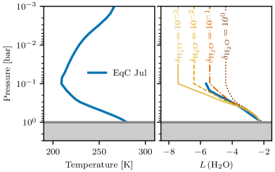
Retrievals commonly assume that the atmospheric trace-gas abundances are vertically constant. While this assumption helps reduce the computational complexity, recent studies have shown that it can bias the retrieved posteriors (e.g., Rowland et al., 2023). For Earth, \ceH2O has strong spectral features throughout the MIR (e.g., Figure 1 in Konrad et al., 2022). The bulk of Earth’s MIR emission originates from the lowermost atmospheric layers (between 1 bar and 0.1 bar), where the atmospheric \ceH2O content decreases strongly with altitude by more than 3 orders of magnitude (see, e.g., Figure 1; Mettler et al., 2024). The main process responsible for this decrease in \ceH2O in Earth’s lower atmosphere is the convection of moist air from the surface to higher atmospheric layers. The rising moist air cools causing \ceH2O to condense, form clouds, and rain out. Consequentially, the \ceH2O abundance drops significantly with altitude in Earth’s atmosphere, and we expect signatures thereof to be imprinted in the MIR emission.
To model the condensation induced vertical variations in the \ceH2O profile in our retrieval forward model, we start by calculating the saturation vapor pressure of \ceH2O for each atmospheric layer. For this, we use the temperature of the layer as well as one of the two experimentally determined Goff-Gratch equations (Eqs. 2 and 3; Goff & Gratch, 1946; Goff, 1957). If is greater than the triple point temperature of \ceH2O ( K), we use the equation for the saturation vapor pressure over water ( in hPa):
| (2) |
Here, K and hPa are the steam-point temperature and pressure of \ceH2O, and the factors are constants: , , , , , and . Conversely, if lies below , we use the Goff-Gratch equation for the saturation vapor pressure over ice ( in hPa):
| (3) |
Here, hPa is the triple point pressure of \ceH2O, and the factors are constants: , , and . The vapor pressure of \ceH2O () as a function of can be summarized as:
| (4) |
Next, we assume a vertically constant volume mixing ratio of \ceH2O (). Starting from the surface layer, we follow the atmospheric PT structure to the higher atmospheric layers with pressures and temperatures . For each layer, we compare the partial pressure of \ceH2O () to . If lies below , we proceed to the next layer. In contrast, if in a layer exceeds , we reduce in that layer and all lower-pressure layers such that in the current layer equals . This yields a profile that is either constant or decreasing with altitude (depending on the PT structure and in the surface layer).
This condensation model accurately estimates in Earth’s lower troposphere ( bar), where is comparable to . However, it significantly overestimates the in Earth’s dry upper troposphere and stratosphere ( bar), where is significantly smaller than . In our retrievals, we allow for a dry upper atmosphere by adding a drying parameter, , to the forward model. Using the parameter , we calculate the dried \ceH2O profile, , as follows:
| (5) |
Here, is in the uppermost atmospheric layer. Equation 5 is designed such that the drying is strongest for small values of and for atmospheric layers where is comparable to . A value of results in , which means that there is no drying in the upper atmosphere.
In Figure 1, we demonstrate that our condensation model yields realistic estimates for Earth’s \ceH2O profile. We compare the ground truth \ceH2O profile for the disk-integrated average equatorial view of Earth in July (EqC Jul) with \ceH2O profiles that we calculated from the EqC Jul PT structure using our condensation model and different values (see Section 2.3.2 for information on the EqC Jul view). We observe that our condensation model successfully approximates Earth’s true \ceH2O profile for . The value of mainly affects the \ceH2O profile for bar and is required to accurately model Earth’s \ceH2O structure. If drying is neglected (brown-dotted line; ), we fail to accurately reproduce Earth’s \ceH2O profile.
2.1.2 Model for partial cloud coverage
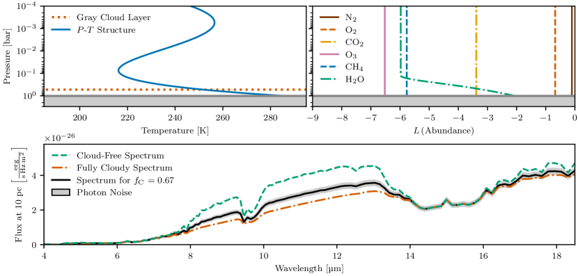
The condensation of \ceH2O in Earth’s atmosphere is linked to the formation of \ceH2O clouds. Thus, if \ceH2O condenses in our model atmosphere, we expect clouds to form. To account for this effect, we add the option to include a simple model for partial cloud coverage in the retrieval forward model.
To account for clouds in our retrievals, we position gray clouds at an atmospheric pressure of . We calculate by taking the median pressure of all atmosphere layers where \ceH2O condensation occurs that exhibit a relative humidity greater than 10% (i.e., ). This assumption for positions the clouds within the atmospheric layers where \ceH2O condenses. If no \ceH2O condensation occurs, we assume the atmosphere to be cloud-free.
To model an Earth-like partial cloud cover, we use our retrieval forward model to calculate the spectra for a cloud-free () and cloudy () model atmosphere. We then mix the two spectra as follows to obtain the total flux as a function of the wavelength :
| (6) |
Here, the forward model parameter describes the cloud-fraction. A value of corresponds to the cloud-free case, whereas yields a fully cloudy atmosphere.
2.2 Retrieval forward models
| Model | Color-coding | Model description |
|---|---|---|
| Vertically constant \ceH2O abundance, cloud-free | ||
| \ceH2O abundance from condensation model, cloud-free | ||
| \ceH2O abundance from condensation model, partial cloud coverage |
| Parameter | Description | Validation True Values | Prior | Model Configuration | ||
|---|---|---|---|---|---|---|
| PT parameter (degree 4) | 1.69 | |||||
| PT parameter (degree 3) | 23.12 | |||||
| PT parameter (degree 2) | 99.70 | |||||
| PT parameter (degree 1) | 146.63 | |||||
| PT parameter (degree 0) | 285.22 | |||||
| 0.01 | ||||||
| Planet radius | 1.00 | |||||
| 0.00 | ||||||
| -0.10 | ||||||
| -0.68 | ||||||
| -3.39 | ||||||
| -6.52 | ||||||
| -5.77 | ||||||
| -2.10 | ||||||
| -2.00 | ||||||
| Cloud fraction | 0.67 | |||||
Note. — The second column shows the color-coding used for the models throughout this publication.
Note. — Here, stands for . In the third column we specify the values assumed to generate the mock-Earth spectrum for the validation retrievals. The listed \ceH2O value is the abundance at the surface obtained from the condensation model. The value is motivated by the average cloud fractions presented in Mettler et al. (2024) and is chosen such that the calculated \ceH2O profile fits Earth’s profile. All other parameter values are taken from Konrad et al. (2022). In the fourth column, the assumed priors are listed. We denote a boxcar prior with lower threshold and upper threshold as ; For a Gaussian prior with mean and standard deviation , we write . The last three columns summarize the model parameters used by the different retrieval forward models ( used, unused).
We run retrievals using the three different forward models listed in Table 2. A complete list of the parameters used by each model is provided in Table 3. All models assume a 1D atmosphere consisting of 100 equally thick layers (in log-space) between bar and the surface pressure . Each individual layer is characterized by its pressure , the corresponding temperature , and the opacity sources present. As in Konrad et al. (2022, 2023), Alei et al. (2022b, 2024), and Mettler et al. (2024), we parameterize the atmospheric PT structure by means of a fourth order polynomial:
| (7) |
The factors are the five forward model parameters describing the atmospheric PT structure. This choice is motivated by Konrad et al. (2022), who demonstrate that a polynomial PT model helps reduce a retrieval’s computational complexity by minimizing the number of PT parameters222In a recent publication, Gebhard et al. (2023) demonstrated that learning-based PT models can reduce the number of PT parameters further. However, the accuracy of such models for terrestrial PT structures is currently limited by the availability of sufficient training data..
Further, all models assume the same spectroscopically active molecules to be present. We model MIR molecular absorption and emission features of \ceCO2, \ceH2O, \ceO3, and \ceCH4333This choice of molecules is motivated by a detailed Bayesian model comparison study performed by Mettler et al. (2024) for the same disk-integrated Earth spectra.. The used line lists, broadening coefficients, and cutoffs are summarized in Table 2.2. We also consider collision-induced absorption (CIA) and Rayleigh scattering features of atmospheric molecules (all considered CIA-pairs and Rayleigh-species are summarized in Table 2.2). Further, we use a spectroscopically inactive filling gas with the mean molecular weight of \ceN2 to ensure that: . Last, to determine the scale height of the model atmosphere, we require the planetary surface gravity, which we calculate from the radius and mass parameters (, ).
The three forward models only differ in the assumptions made for the \ceH2O abundance profile and the clouds. The simplest model () assumes constant abundance profiles for all molecules and a cloud-free atmosphere. This model is equivalent to the forward model used in Mettler et al. (2024). The intermediate complexity model () again assumes the atmosphere to be cloud-free. However, it allows for a non-constant \ceH2O abundance profile by modeling \ceH2O condensation as described in Section 2.1.1. The most complex of the three models () also accounts for \ceH2O condensation. In addition, it relaxes the assumption of a cloud-free atmosphere by modeling partial cloud coverage following the method outlined in Section 2.1.2.
| Molecular Line Opacities | CIA | Rayleigh Scattering | |||||||
|---|---|---|---|---|---|---|---|---|---|
| Molecule | Line List | Pressure-broadening | Wing cutoff | Pair | Reference | Molecule | Reference | ||
| \ceCO2 | HN20 | 25 cm-1 | \ceN2\ceN2 | KA19 | \ceN2 | TH14, TH17 | |||
| \ceH2O | HN20 | 25 cm-1 | \ceN2\ceO2 | KA19 | \ceO2 | TH14, TH17 | |||
| \ceO3 | HN20 | 25 cm-1 | \ceO2\ceO2 | KA19 | \ceCO2 | SU05 | |||
| \ceCH4 | HN20 | 25 cm-1 | \ceCO2\ceCO2 | KA19 | \ceCH4 | SU05 | |||
| … | … | … | … | \ceCH4\ceCH4 | KA19 | \ceH2O | HA98 | ||
| … | … | … | … | \ceH2O\ceH2O | KO21 | … | … | ||
| … | … | … | … | \ceH2O\ceN2 | KO21 | … | … | ||
2.3 Input spectra for the retrievals
In the context of this study, we consider two different types of input spectra. All considered spectra are characterized by their spectral resolving power () and signal-to-noise ratio (). We define the of a spectrum as , where is the width of a given wavelength bin and the wavelength at the bin’s center. We introduce the simulated 1D Earth spectrum used to test the different forward models in Section 2.3.1. Next, in Section 2.3.2, we provide information on the empirical, disk-integrated Earth spectra and the corresponding ground truths studied in the main analysis of this work. Last, we provide details on the assumptions made for the wavelength dependent of all spectra in Section 2.3.3.
2.3.1 Simulated 1D Earth spectrum
Before performing retrievals on real, disk-integrated Earth spectra, we run test retrievals with all forward models on a simulated spectrum of a 1D Earth-like atmosphere to validate our approach. We generate the 1D Earth spectrum using the cloudy forward model (see Section 2.2). We assume an Earth-like PT structure, radius, mass, and atmospheric composition (see Table 3 and Figure 2). The atmospheric \ceH2O content is determined with the condensation model by assuming . For the cloud fraction, we assume , which corresponds to the lower limit for the mean annual cloud fractions of the Earth views in Mettler et al. (2024) (range: ). We calculate the spectrum for the minimal LIFE wavelength range () specified in Konrad et al. (2022), choose a spectral resolving power of , and assume photon-noise (low-noise model in Section 2.3.3). We show the obtained simulated MIR Earth spectrum in the bottom panel of Figure 2.
2.3.2 Real disk-integrated Earth spectra and ground truths
As input for the main retrieval analysis of this study, we use the same set of monthly averaged444We consider monthly averages since this time span roughly corresponds to the expected LIFE integration times specified in Konrad et al. (2022). disk-integrated Earth spectra as in Mettler et al. (2024). The spectra are derived from Earth remote sensing climate data from NASA’s Atmospheric Infrared Sounder (AIRS; Chahine et al., 2006) aboard the Aqua satellite. We refer to Mettler et al. (2023) and Mettler et al. (2024) for a description of the methods used to derive these disk-integrated, monthly averaged Earth spectra.
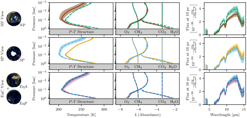
The spectra cover the wavelength range, with a gap at due to dead instrument channels. We consider three different orientations of Earth relative to the observer. For the North (NP) and South Pole (SP) case, the respective polar region is centered on the observed disk. The Equatorial Combined (EqC) view is centered on Earth’s equator and is the combination of an Africa-centered (EqA) and a Pacific-centered (EqP) equatorial view. We combine the EqA and EqP views into the EqC spectrum to account for Earth’s rotation, which is significantly faster than the assumed 1-month integration time. To capture Earth’s largest variability, we consider the monthly averages for January (Jan) and July (Jul) from 2017 for each orientation. This yields a total of six different Earth spectra.
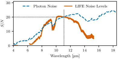
Motivated by first LIFE requirement estimates from Konrad et al. (2022) (, ), we consider two resolving powers () and two noise levels () for each spectrum. With the LIFE noise model from Section 2.3.3, we determine the wavelength-dependent of the disk-integrated spectra. In Figure 3 we show all six disk-integrated Earth Spectra for the , case.
In Section 3, we compare the retrieved posteriors with ground truth averages for the different views. The ground truths for the PT profiles and the trace gas abundances of \ceH2O, \ceCH4, and \ceO3 were derived from the Aqua/AIRS L3 Monthly Standard Physical Retrieval (AIRS-only) 1 degree x 1 degree V7.0 product (AIRS Project, 2020). Ground truth averages for \ceCO2 were calculated from the OCO-2 GEOS Level 3 monthly dataset (0.5x0.625 assimilated \ceCO2 V10r at GES DISC; NASA/GSFC/GMAO Carbon Group, 2021), which is derived from observations from the Orbiting Carbon Observatory 2 (OCO-2). We display the ground truths for all views and months in Figure 3. For details on the calculation of these disk-integrated ground truths, we refer to Mettler et al. (2024).
2.3.3 Considered noise models
In the present study, we use two different approaches to model the wavelength-dependent of the considered MIR spectra. First, to test the different forward models on the simulated Earth spectrum, we assume a low-noise scenario. Second, for the retrievals on the disk-integrated Earth spectra, we use a more realistic LIFE-like model. Because the is not constant over the spectrum for both cases, we define the of the spectrum as the in the wavelength bin (see Figure 4). We choose the bin since it does not coincide with strong absorption features and thus probes Earth’s continuum emission. This reference wavelength was also used by previous LIFE-related retrieval studies (Konrad et al., 2022; Alei et al., 2022b; Konrad et al., 2023; Mettler et al., 2024; Alei et al., 2024).
For the low-noise scenario, we only assume photon noise of the source to be present. Thus, if photons are detected in a given wavelength bin, we assume the noise to be . To calculate the , we scale the flux such that the desired is reached at . The wavelength-dependent photon noise is indicated by the blue-dashed line in Figure 4.
To obtain the more realistic LIFE-like noise estimates, we use the LIFEsim model (Dannert et al., 2022). In addition to accounting for photon noise of the planet emission, LIFEsim models contributions from major astrophysical noise sources (stellar leakage and local- as well as exozodiacal dust emission). Thus, LIFEsim makes the implicit assumption that observations with a LIFE-like instrument will not be dominated by instrumental noise terms (Dannert et al., in prep.; Huber et al., in prep.). To calculate the LIFEsim noise, we assume the observed planet to orbit a G2V star at AU at a separation of pc from us. The exozodiacal dust emission is set to three times the local zodiacal dust emission, which is the median exozodi emission found for Sun-like stars by the HOSTS survey (Ertel et al., 2020). The wavelength-dependence of the LIFEsim noise we assume for the disk-integrated Earth spectra is indicated by the solid-red lines in Figure 4.
For all spectra, we treat the wavelength-dependent as uncertainty on the flux. This implies that the spectral points are set to the true flux values and are not randomized according to the . While randomized spectra provide more accurate simulated observations, retrievals on such noise realizations yield biased parameter posteriors. Ideally, our retrieval study would consider a large number () of different noise realizations of one spectrum. However, such a study is computationally unfeasible due to the large number of required atmospheric retrievals. Alternatively, as motivated in Konrad et al. (2022), retrievals on unrandomized spectra can be used to obtain estimates for the average expected retrieval performance for randomized spectra.
2.4 Prior distributions of model parameters
All prior distributions assumed to run the retrievals are listed in Table 3. We choose the priors for the PT parameters and the surface pressure such that the resulting PT structures cover a wide range of profiles (from cold and thin Mars-like to hot and massive Venus-like atmospheres). For the atmospheric gases \ceN2, \ceO2, \ceCO2, \ceO3, and \ceCH4, we assume broad uniform priors in log-space that extend from to in mass fraction. The lower limit of lies significantly below the estimated minimal detectable abundances presented in Konrad et al. (2022) ( in mass fraction).
Based on the retrieved abundance constraints form Mettler et al. (2024), we exclude \ceH2O dominated atmospheres by setting the upper limit of for the \ceH2O prior. For planets on Earth-like orbits around G-stars, high \ceH2O abundances can occur for high partial pressures of \ceCO2 ( bar) or other greenhouse gases due to the increased surface temperature (e.g., Wordsworth & Pierrehumbert, 2013). Yet, such atmospheres lie close to the critical runaway greenhouse limit and are out of scope for this study. For the parameter, we choose a log-uniform prior between to . This allows for atmospheric \ceH2O to deplete by up to five orders of magnitude in the upper atmosphere. Further, the uniform prior between 0 and 1 covers the full range from cloud-free to fully cloudy atmospheres.
We assumed Gaussian priors for the planet radius and mass . The prior is motivated by Dannert et al. (2022), who find that already the detection of a planet with LIFE yields a first estimate. For terrestrial planets in the HZ, they predict a radius estimate for the true radius of . We derive the prior for from the prior using the statistical mass-radius relation Forecaster (Chen & Kipping, 2016). These and priors are in accordance with previous LIFE-related retrieval studies (Konrad et al., 2022, 2023; Alei et al., 2022b; Mettler et al., 2024).
3 Retrieval Results
In the following, we present the results from the validation retrievals on the simulated 1D Earth spectrum in Section 3.1. Thereafter, the findings from the retrievals on the six empirical disk-integrated Earth views are presented in Section 3.2.
3.1 Results for the simulated 1D Earth spectrum
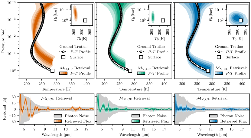
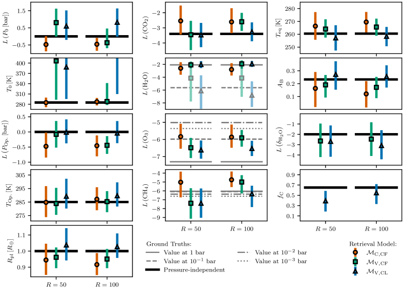
We present the retrieval results for the simulated 1D Earth spectrum (Section 2.3.1) using the three retrieval models , , and (Table 2, Section 2.2). In Figure 5, we illustrate the constraints retrieved for the PT structure and the surface conditions. For the model, the retrieved PT structure is shifted to lower pressures relative to the ground truth. On average, the surface temperature is underestimated by K and the surface pressure by dex (‘dex’ reports the value of a quantity in log-space: dex; Unit). With the model, which accounts for \ceH2O condensation, these shifts are significantly reduced and the ground truth lies within the 1- envelope of the retrieved PT structure. Yet, remains slightly underestimated ( dex) and the constraint is not improved. The model, which assumes a partial cloud coverage, yields the most accurate constraints for the PT structure. The true lies within the 16%-84% percentile range of the posterior ( dex). The estimate for is also improved significantly, but the uncertainty is increased ( K).
The flux residuals in Figure 5 show that the model fails to accurately fit the input spectrum. Especially in the strong absorption features of \ceH2O (), \ceO3 (), and \ceCO2 (), the fitted flux differs significantly from the input, which indicates these features cannot be modeled correctly. In contrast, the retrieval provides an accurate fit to the input spectrum above , which is in agreement with the improvements observed for the PT structure. Finally, the model yields further minor improvements over the model in the high noise regime of the input spectrum between .
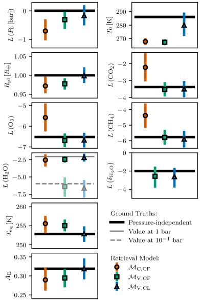
In Figure 6 and Table 5, we summarize the retrieved posteriors for the forward model parameters. We provide the posteriors for the surface conditions, the planet radius , the atmospheric trace gases, the drying parameter , and the cloud fraction . The posteriors are visualized by the retrieved PT structures in Figure 5. The posteriors for , \ceN2, and \ceO2 are not shown, since they were not constrained over the assumed priors. Last, we derived estimates for the planet’s equilibrium temperature and Bond albedo from the posteriors. For , we calculated the MIR spectra corresponding to the points in the posterior and integrated these spectra to obtain the total MIR emission. We then defined as the temperature of a spherical black-body with radius that emits the same total flux. From , we then determined :
| (8) |
Here, is the exoplanet’s semi-major axis and the star’s luminosity. For details on the derivation of and , we refer to Mettler et al. (2024).
| Parameter | Ground | Posteriors | ||
|---|---|---|---|---|
| Truths | ||||
| … | ||||
| … | … | |||
Note. — Here, stands for . The second column lists the assumed ground truths (see Table 3 for details). In the last three columns, we list the median and the range (via indices) of the parameter posteriors for the , , and models. For \ceH2O, all listed values correspond to the surface-layer abundances.
As seen for the PT structures, both the and posteriors are biased relative to the ground truth for the retrieval. Due to a degeneracy between the pressure-induced line-broadening and the abundances of the atmospheric trace-gases (see, e.g., Misra et al., 2014; Schwieterman et al., 2015; Alei et al., 2022a), we expect the underestimation of the pressures to be accompanied by an overestimation of the trace-gas abundances. Indeed, the \ceCO2, \ceO3, and \ceCH4 abundances are overestimated by dex to dex by the retrieval. For the and retrievals, which yield better pressure constraints, the abundance estimates are unbiased (i.e., the ground truths fall within the 16%-84% posterior range). Only the \ceH2O abundance, which decreases strongly with altitude in Earth’s atmosphere, is not overestimated by the retrieval. The retrieved abundance lies between the 1 bar and bar ground truth, roughly dex below the surface abundance (see Table 5). For the retrieval, the abundance at bar is accurately estimated. Yet, since and are underestimated, the condensation model underestimates the surface \ceH2O abundance by dex. With the model, this bias on the surface abundance of \ceH2O is removed. The estimates from the and scenarios do not differ significantly. In both cases, values of are ruled out. Thus, an Earth-like \ceH2O depletion in the upper atmosphere is in principle detectable from the MIR thermal emission.
Similar to , is underestimated by by the and retrievals. This bias is propagated to the and estimates, since they are derived from the posterior. For the and retrievals, the underestimated translates to an overestimated (by K) and an underestimated (by ). Thus, a too small is compensated with an increased , which requires a lower . In contrast, the retrievals using the true model yield accurate and bias-free estimates for , , and .
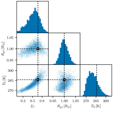
Last, in the retrievals, we aim to constrain the cloud fraction . We show the , , and posteriors from the retrieval in the corner plot in Figure 7. While is not strongly constrained over the prior range, we observe significant correlations between and the other parameters. The correlation between and implies that a higher can be compensated with a higher , since atmospheric clouds block the thermal emission from the warm near-surface layers. This degeneracy explains the observed increase in the uncertainty for the retrieval. Further, is weakly correlated with (higher lead to higher ), which explains why estimates are improved for the model.
Finally, we use Bayes’ factor (values in Table 6) to benchmark the models against each other. We find that is preferred over (), and outperforms (). Thus, an accurate model for Earth’s \ceH2O abundance profile is required to correctly fit its MIR spectrum. This agrees with our findings for the retrieved PT structures, flux residuals, and parameter posteriors. Further, is slightly preferred over the cloud-free model (). This slight preference agrees with the small improvements observed for the flux residuals. Yet, despite the limited improvements in the spectral fit, the degeneracies associated with help improve the estimates for , , , and .
3.2 Results for real disk-integrated Earth spectra
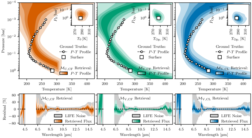
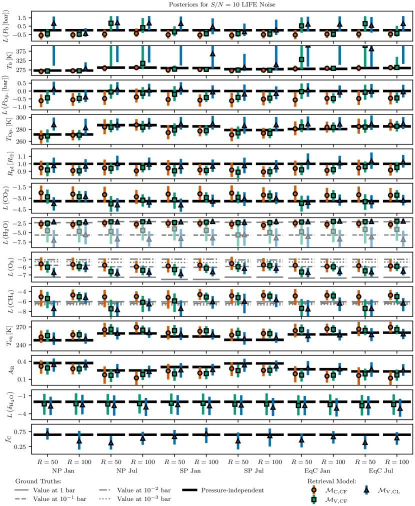
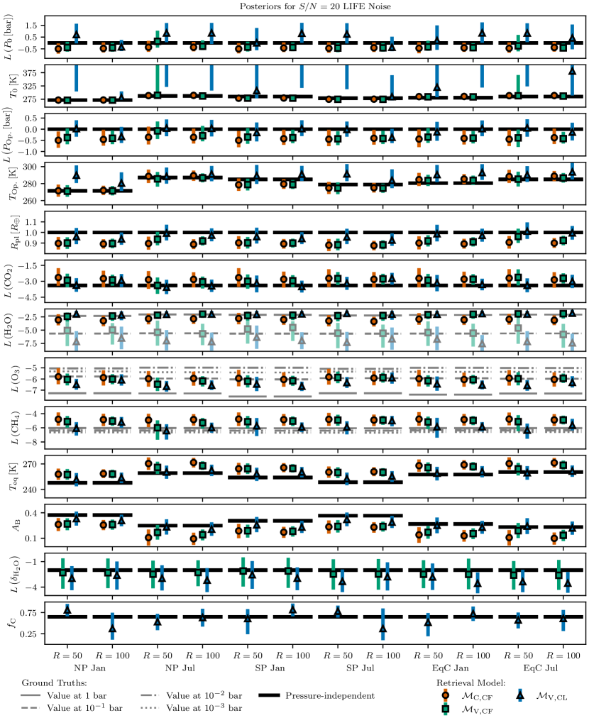
Here, we present the retrieval results for the empirical disk-integrated Earth views (Section 2.3.2) for the , , and retrieval models (Table 2, Section 2.2). In Figure 8, we show the retrieved PT structures for the , EqC Jul Earth spectrum. Further, we show the residuals of the fitted spectra relative to the input spectrum. The PT results and the residuals for all other views, , and scenarios are comparable and thus not shown.
The PT structures retrieved for the model exhibit similar characteristics as the results for the simulated spectrum. The retrieved constraints are systematically shifted toward lower pressures. Also is underestimated by dex to dex depending on the view. In contrast, is well approximated by the retrievals (truths lie in the posterior range). While shifts in the retrieved PT profiles relative to the ground truth are also observed for , the runs yield accurate constraints. However, for both and , the PT constraints, which extend significantly beyond the true and , indicate that the surface conditions are no longer well constrained. This suggests that the high-pressure layers of the fitted model atmosphere do not contribute significantly to the MIR thermal emission emerging at the top of the atmosphere. Alternatively, we can consider the pressure () and temperature () in the deepest layer in the model atmosphere that still contributes to the simulated MIR spectrum. Thus, and correspond to the pressure and temperature at which the simulated atmosphere becomes opaque in the MIR. For an optically thin atmosphere, we simply obtain: and . We observe that and roughly correspond to the ground truths for and . Thus, the fitted model atmospheres become opaque close to Earth’s true surface.
The flux residuals in Figure 8 do not differ significantly between the models. Around the \ceN2O band, the models struggle to fit the spectrum accurately, since they do not include \ceN2O. Mettler et al. (2024) showed that, for the empirical disk-integrated Earth spectra we consider here, models including \ceN2O are not preferred by Bayesian model selection. At all other wavelengths, the three models provide an accurate fit. This observation is supported by model comparison via the Bayes factor (values in Table 6). For all and most spectra, no model is preferred over the others (; uncertainty ). Rare exceptions occur for the , spectra, where slight preferences for or are occasionally observed (; uncertainty ).
In Figure 9, we visualize the posteriors retrieved with the , , and models for the EqC Jul view at a LIFEsim of . The results for the other views and the retrievals exhibit the same general behavior and are provided in Figures 10 and 11 in Appendix A. Further, the numeric values for all posteriors are listed in Tables 7, 8, and 9. We show the posteriors for , , , , , the trace-gas abundances, , and . The posteriors are visualized via the PT constraints in Figure 8. We do not show the , \ceN2, and \ceO2 posteriors, since they are not constrained over the assumed priors. The and estimates were derived from the posteriors (see Section 3.1).
We observe that the posteriors for the different models exhibit trends similar to the ones observed for the simulated 1D Earth spectra in Section 3.1. For the model, the underestimated values are accompanied by overestimated abundances of \ceCO2 (by dex) and \ceCH4 (by dex). For \ceO3, the pressure-dependent ground truths cover a wide range of abundances. Thus, the pressure-induced biases are not directly observable. Next, the posteriors for \ceH2O underestimate the true surface-layer abundances by dex to dex. Further, is consistently underestimated by , which translates to biases for the derived parameters and ( overestimated by K; underestimated by ). Only is accurately estimated by for most scenarios.
For and , significant improvements in the parameter estimates are observable. Generally, the estimates are higher than for the runs. As seen with the PT profiles, several and retrievals only yield lower limits for and . In these cases, the value indicates that the high-pressure layers of the model atmosphere do not contribute to the MIR spectrum and thus and cannot be constrained further. The retrieved estimates increase with the model complexity and mostly coincide with the ground truth for the retrievals. Further, provides accurate estimates for in the retrievals. For , generally overestimates and the uncertainties are often significantly increased. This is due to the aforementioned degeneracy between and , where too high can be compensated by a higher . Also, the retrieved estimates for and the derived parameters and are significantly improved, especially for the retrievals.
For the trace-gas abundances, the biases observed for the retrievals are continually reduced as we include \ceH2O condensation and clouds. The model yields the best estimates for the atmospheric \ceCO2 abundances. For all cases considered, the \ceCO2 ground truths lie in the percentile range of the posteriors. Also for \ceCH4, the biases are reduced and the posteriors estimate the ground truths accurately for most scenarios. Yet, for some , scenarios, \ceCH4 is no longer detectable. In these cases, only an upper limit is obtained for the \ceCH4 abundance ( dex). For \ceO3, we observe a significant reduction in the retrieved abundance. This indicates that the \ceO3 estimate in the retrieval is affected by the same pressure-abundance degeneracy as \ceCO2 and \ceCH4. Last, the \ceH2O abundance at provides accurate estimates for Earth’s ground truth surface abundance of \ceH2O. Further, the structure of the \ceH2O profile is accurately approximated by both the and retrievals.
Lastly, all retrievals yield similar constraints for and independent of the disk-integrated Earth spectrum considered. As for the simulated Earth spectrum in Section 3.1, only high values of can be ruled out for both the and the model. Further, the retrievals often struggle to constrain due to the aforementioned correlations with . Generally, values of are retrieved and only lower than can be ruled out confidently. In some retrievals, the lower limit obtained for is significantly higer (lower limit on : ).
4 Discussion
Here, we outline implications of our work for the characterization of terrestrial HZ exoplanets (Section 4.1) and for the LIFE mission requirements (Section 4.2). Thereafter, in Section 4.3, we point out the limitations of the present study.
4.1 Implications for Characterizing Rocky HZ Exoplanets
We find that the biased estimates for the PT structure and the atmospheric composition obtained in the retrievals are predominantly attributable to two simplifying assumptions commonly made by retrieval models: vertically constant abundance profiles and a cloud-free atmosphere. Our results for the and retrieval models demonstrate that including physically motivated models for Earth’s atmospheric \ceH2O profile and partial cloud coverage helps significantly improve the accuracy of the retrieved parameter estimates. However, despite the improved parameter estimates, neither the nor the model is preferred over the model by Bayesian model comparison for LIFE-like and scenarios. Yet, we argue that the usage of the and models is justifiable, since both impose physics informed constraints on the model atmosphere. This allows to exclude unrealistic atmospheric states and thereby yields more reliable parameter estimates. Especially for HZ exoplanets, unbiased parameter constraints are a critical requirement to enable the accurate assessment of their habitability. Further, in the same context, biased estimates for the abundances of potential biosignature gases, such as \ceCH4, can be highly problematic.
From Figure 3 and Mettler et al. (2023), we know that Earth’s MIR emission spectrum depends significantly on both the observed view and the season. Since both the viewing geometry and the season will be unknown for future observations of HZ terrestrial exoplanets, it is crucial to understand if and how these factors affect our characterization. We find that, independent of the assumed retrieval model, the retrieved constraints for most of the model parameters exhibit no significant dependence on the view and season of the Earth spectrum. Only , , , and exhibit a perceptible dependence on the considered spectrum in the high and scenarios (see Figures 10 and 11). These findings are in agreement with Mettler et al. (2024), who performed retrievals on the same set of disk-integrated Earth spectra considered here using the forward model.
4.2 Implications for the LIFE Initiative
Several retrieval studies have evaluated how well rocky HZ exoplanets could be characterized from their MIR spectrum by a LIFE-like observatory. In Konrad et al. (2022), preliminary minimal requirements for LIFE are obtained by analyzing simulated Earth spectra. By requiring a detection of the potential biosignature \ceCH4 with LIFE, the authors find lower limits of for the wavelength coverage, for , and for . In two follow-up studies (Alei et al., 2022b; Konrad et al., 2023), these findings are reevaluated on simulated spectra of Earth at different temporal epochs from Rugheimer & Kaltenegger (2018) and a cloudy Venus-like planet. Last, Mettler et al. (2024) test the LIFE requirements on the same real disk- and time-averaged MIR Earth spectra we considered here.
While the analyzed spectra vary significantly in complexity, all previous studies assumed retrieval models with vertically constant abundance profiles. Further, only Konrad et al. (2023) accounted for clouds in their retrieval models. All studies yield similar results for the strengths of the parameter constraints and the detectability of trace-gases. They find Earth-like levels of \ceH2O, \ceCO2, \ceO3, and \ceCH4 to be detectable. Further, the retrieved posterior range does not exceed dex for pressures, K for temperatures, for , and dex for trace-gas abundances. These constraints from the previous LIFE studies are consistent with our results for the retrieval model, which also assumes constant abundance profiles and neglects clouds.
However, similar to our findings for retrievals, both Alei et al. (2022b) and Mettler et al. (2024) observe significant biases in the retrieved posteriors relative to the ground truths. Both studies analyzed spectra of cloudy atmospheres with non-constant trace-gas abundances. Mettler et al. (2024) argue that underestimated pressures and overestimated trace-gas abundances are primarily evoked by the retrieval model assumption of a vertically constant \ceH2O profile. In contrast, biased temperature, , and estimates are attributable primarily to neglecting clouds. Our findings for the simulated Earth spectrum (Section 3.1) validate these claims. In the retrievals, biases on pressure and abundance estimates are reduced significantly by modeling Earth’s \ceH2O abundance profile. Yet, temperature, , and estimates are largely unaffected. These biases are only reduced in the cloudy retrievals. Also our findings for the real disk-integrated Earth views (Section 3.2) validate the claims from Mettler et al. (2024) by exhibiting similar bias reductions. However, the improved estimates for individual parameters are no longer attributable to solely the variable \ceH2O profile or the inclusion of clouds.
We observe two additional important differences between the and retrieval results and the previous studies. First, we do not retrieve accurate estimates for and for most views independent of the and of the spectrum. The retrieved \ceH2O profiles indicate that the \ceH2O abundance in the lower atmosphere is increased by dex compared to the model. These elevated \ceH2O levels lead to an optically thick lower atmosphere due to the strong MIR continuum opacity of \ceH2O. As a result, the high-pressure layers of the model atmosphere do not contribute to the exoplanet’s MIR spectrum and therefore only lower limits for and are attainable. The pressure of the lowest atmosphere layer that still contributes to the modelled MIR spectrum roughly corresponds to the ground truth value. Thus, the model atmosphere becomes opaque to MIR radiation close to Earth’s surface. This agrees well with measurements of the MIR opacity of Earth’s atmosphere (see, e.g., Harries et al., 2008). This finding can be generalized to exoplanets, where clouds and the MIR opacity sources set a fundamental limit on how deep an atmosphere can be probed.
Second, at the minimal and requirements from Konrad et al. (2022) (, ), Earth-like \ceCH4 mass fractions of are not reliably detected in the and retrievals. Instead, most of these retrieval runs yield upper limits of dex for the \ceCH4 abundance. This occurs since Earth’s main MIR \ceCH4 signature at overlaps with a strong \ceH2O band (). Thus, changes to the \ceH2O abundance model directly impact the \ceCH4 retrieval. Importantly, the main driver for the initial and requirements was the capability to detect \ceCH4 in an Earth-like atmosphere. Our results indicate that a bias-free constraint on the \ceCH4 abundance (mean of \ceCH4 posterior within dex of 1 bar ground truth; uncertainty dex) at is only possible for . For the scenarios, such \ceCH4 constraints remain possible for .
Last, while the simulation-based LIFE studies analyzed the MIR emission between , the empirical Earth spectra studied here and in Mettler et al. (2024) cover a smaller range (, ). Yet, the constraints we retrieved for the model are comparable to the previous studies. This suggests that measurements of the MIR flux above and between are not essential to accurately characterize an exo-Earth with LIFE. However, additional studies are required to investigate whether this finding generalizes to arbitrary HZ terrestrial exoplanets.
4.3 Limitations and Future Work
The present study demonstrates, that adding simple physical constraints to the retrieval forward model can help significantly reduce biases in the retrieved posteriors for an Earth-like spectrum. Yet, there are limitations inherent to our work, the effect of which must be investigated in future studies.
First, our model for the atmospheric \ceH2O profile assumed that condensation occurs if the relative humidity reaches 100%. Thus, physical tropospheric states, such as the \ceH2O supersaturation of air (e.g., Spichtinger et al., 2003; Genthon et al., 2017), are not possible. Yet, since we are only sensitive to order of magnitude changes in the \ceH2O abundance for the and scenarios considered, we do not expect such factors to significantly affect our findings. Further, we assumed that only condensation affects the \ceH2O profile. However, in the stratosphere and above, the \ceH2O abundance is strongly affected by additional processes such as the photochemical oxidation of \ceCH4 (e.g., Jones et al., 1986; Frank et al., 2018). Yet, since the bulk of Earth’s MIR emission originates from the troposphere, we argue that the stratospheric \ceH2O profile only affects our characterization negligibly.
Second, we assume constant abundance profiles for all trace-gases except for \ceH2O. On Earth, especially the \ceO3 but also the \ceCH4 abundances exhibit significant altitude dependencies (see Figure 3). These variations are predominantly evoked by photochemical processes in the stratosphere (Chapman, 1932; Jones et al., 1986). However, in contrast to \ceH2O, a simple physical constraint for the \ceO3 and \ceCH4 profiles does not exist (e.g., Kozakis et al., 2022). As a result, models for these profiles would be relatively unconstrained. In addition, the MIR spectral feature of \ceO3 at originates from the high pressure layers in Earth’s atmosphere ( bar). Consequentially, we are not sensitive to the large \ceO3 variations in the upper atmosphere at the considered and . Also for \ceCH4, the main contribution to the MIR feature at originates from the high pressure layers ( bar). The vertical variations in the ground truths in these layers ( dex) are significantly smaller than the uncertainties on the \ceCH4 posteriors ( dex). Given the limited spectral information available, the impact of the \ceO3 and \ceCH4 variations on our results is likely negligible.
Third, instead of modelling the wavelength-dependent MIR opacity of \ceH2O clouds, we assume gray clouds. Further, we assume the clouds to form in a single atmosphere layer. In contrast, for Earth, the position of the cloud-top is variable ( ranges from bar; e.g., Kokhanovsky et al., 2011). However, the MIR optical properties of clouds do not vary strongly with wavelength or pressure (Petty, 2006). Furthermore, findings presented in Konrad et al. (2023) suggest that physical cloud properties (such as cloud composition and particle size) cannot be constrained for the LIFE and scenarios considered here. Thus, given the limited information content of the spectra studied, the assumption of gray clouds at a fixed height is justifiable.
Fourth, we parameterized the atmospheric PT profile using a fourth order polynomial. This model has the benefit of being highly flexible. Since it does not impose any physical constraints, it can fit any PT structure. However, limiting the atmospheric PT structure to physically viable states by using a learning-based parametrization (see, e.g. Gebhard et al., 2023) could help improve our characterization. This is especially promising for the and models, since they link the \ceH2O abundance profile and the clouds to the atmospheric PT structure. However, for terrestrial atmospheres, the reliability of learning-based PT models is currently limited by the availability of sufficient training data.
Fifth, we focus on Earth’s MIR emission spectrum, which provides an excellent benchmark (e.g., Robinson & Salvador, 2023). Our finding that neglecting vertical abundance variations and clouds affects the retrieved parameter estimates can be generalized to terrestrial exoplanets. Yet, rocky exoplanets will exhibit atmospheres different from Earth. Thus, detailed studies similar to what Rowland et al. (2023) did for cloudy L-dwarfs are required for terrestrial exoplanets to search for additional model assumptions that could affect the interpretation of MIR thermal emission spectra.
Last, the comparison of different retrieval approaches has revealed that the obtained parameter posteriors can depend on framework particularities such as the radiative transfer implementation, the parameter sampling algorithm, or the used molecular line opacities (e.g., Line et al., 2013; Barstow et al., 2020; Alei et al., 2022a). Community efforts (e.g., the CUISINES Working Group555https://nexss.info/cuisines/) that aim to benchmark, compare, and validate different retrieval frameworks on real and simulated spectral data are indispensable to ensure the correct characterization of HZ terrestrial exoplanet atmospheres in the future.
5 Summary and Conclusions
In this study, we investigated how common atmospheric retrieval assumptions can bias the characterization of terrestrial HZ exoplanets. Specifically, we tested how model assumptions for the vertical \ceH2O abundance profile and the atmospheric clouds impact our characterization of Earth as an exoplanet by running retrievals with different forward models. The baseline model () assumed a cloud-free atmosphere with constant abundance profiles for all trace-gases. While still cloud-free, the model estimated the \ceH2O abundance profile by accounting for \ceH2O condensation. Last, the model allowed for both \ceH2O condensation and a partially cloudy atmosphere. We first validated these three models in test retrievals on a simulated 1D low-noise Earth spectrum (, ). Thereafter, we ran retrievals on LIFE mock observations (; ) of empirical disk-integrated MIR thermal emission spectra of Earth representative of different views and seasons. The performance of the three models was benchmarked against ground truth averages from remote sensing data.
Independent of the assumed forward model, our retrieval results highlight the unique strength of considering an exoplanet’s MIR thermal emission. Earth-like \ceH2O, \ceCO2, and \ceO3 concentrations are easily constrained to within dex, and \ceCH4 is reliably detected at . Further, we significantly constrain the atmospheric PT structure ( dex for pressures, K for temperatures) and the planet radius (). Yet, our results also demonstrate that simplifying assumptions made by retrieval forward models can bias the characterization. For the model, pressures are underestimated by dex, and the abundances of \ceCO2, \ceO3, and \ceCH4 overestimated by dex. Also, the obtained estimates are consistently too low. This translates to biased equilibrium temperature () and Bond albedo () estimates ( K too high; too low). With the forward model, these offsets can already be reduced significantly for most parameters. The model yields bias-free estimates for the shape of the PT structure, , the trace-gas abundances, , and . For the surface pressure and temperature , the and retrievals yield lower limits. For both models, the high-pressure atmosphere layers are opaque to MIR radiation due to their high \ceH2O abundance. Consequentially, these layers do not contribute to the MIR thermal emission spectrum and thus and are not constrainable. These results demonstrate that physically motivated forward models can facilitate the accurate interpretation of spectra.
In addition, our work has important implications for the LIFE technical requirements. Konrad et al. (2022) derived preliminary minimal wavelength coverage, , and requirements by running a grid of retrievals on simulated Earth spectra assuming constant abundance profiles and a cloud-free atmosphere. The authors derived lower requirement limits of , , and by requiring a detection of the potential biosignature \ceCH4. Yet, our results on empirical Earth spectra suggest, that a bias-free \ceCH4 detection is not possible for Earth with the current baseline and requirements. Instead, we find that at a minimal of 100 is required to ensure a confident and bias-free \ceCH4 detection. With a proper treatment of the \ceH2O profile and clouds, an MIR LIFE observation would allow us to correctly identify an exo-Earth as habitable and quantify the abundance of the biosignature gas \ceCH4. Further, our findings suggest that flux measurements above and between are not essential for an accurate characterization of an exo-Earth with LIFE. However, this must be confirmed for non Earth-like HZ terrestrial exoplanets.
First detailed spectral measurements with the JWST have set us off on a journey to characterize and understand the conditions on terrestrial exoplanets. These efforts will intensify with future generations of optimized space missions like LIFE capable of acquiring detailed spectral measurements of nearby temperate terrestrial exoplanets. Inverse modeling approaches such as atmospheric retrievals will be used to analyze these data. Yet, as we demonstrate, simplifying assumptions in retrievals can lead to a biased interpretation. Studies that extend beyond the Earth scenario are essential to build a profound understanding of how different model assumptions may impact the interpretation of observed exoplanet spectra. These efforts are indispensable steps forward in our pursuit of understanding the habitability of distant worlds and are crucial to identifying signs of life outside the Solar System.
References
- AIRS Project (2020) AIRS Project. 2020, Aqua/AIRS L3 Monthly Standard Physical Retrieval (AIRS-only) 1 degree x 1 degree V7.0, NASA Goddard Earth Sciences Data and Information Services Center, doi: 10.5067/UBENJB9D3T2H
- Alei et al. (2022a) Alei, E., Konrad, B. S., Mollière, P., et al. 2022a, in Society of Photo-Optical Instrumentation Engineers (SPIE) Conference Series, Vol. 12180, Space Telescopes and Instrumentation 2022: Optical, Infrared, and Millimeter Wave, ed. L. E. Coyle, S. Matsuura, & M. D. Perrin, 121803L, doi: 10.1117/12.2631692
- Alei et al. (2022b) Alei, E., Konrad, B. S., Angerhausen, D., et al. 2022b, A&A, 665, A106, doi: 10.1051/0004-6361/202243760
- Alei et al. (2024) Alei, E., Quanz, S. P., Konrad, B. S., et al. 2024, arXiv e-prints, arXiv:2406.13037, doi: 10.48550/arXiv.2406.13037
- Angerhausen et al. (2023) Angerhausen, D., Ottiger, M., Dannert, F., et al. 2023, Astrobiology, 23, 183, doi: 10.1089/ast.2022.0010
- Angerhausen et al. (2024) Angerhausen, D., Pidhorodetska, D., Leung, M., et al. 2024, AJ, 167, 128, doi: 10.3847/1538-3881/ad1f4b
- Anglada-Escudé et al. (2016) Anglada-Escudé, G., Amado, P. J., Barnes, J., et al. 2016, Nature, 536, 437, doi: 10.1038/nature19106
- Barstow et al. (2020) Barstow, J. K., Changeat, Q., Garland, R., et al. 2020, MNRAS, 493, 4884, doi: 10.1093/mnras/staa548
- Berta-Thompson et al. (2015) Berta-Thompson, Z. K., Irwin, J., Charbonneau, D., et al. 2015, Nature, 527, 204, doi: 10.1038/nature15762
- Borucki et al. (2010) Borucki, W. J., Koch, D., Basri, G., et al. 2010, Science, 327, 977, doi: 10.1126/science.1185402
- Bowens et al. (2021) Bowens, R., Meyer, M. R., Delacroix, C., et al. 2021, A&A, 653, A8, doi: 10.1051/0004-6361/202141109
- Bryson et al. (2021) Bryson, S., Kunimoto, M., Kopparapu, R. K., et al. 2021, AJ, 161, 36, doi: 10.3847/1538-3881/abc418
- Buchner et al. (2014) Buchner, J., Georgakakis, A., Nandra, K., et al. 2014, A&A, 564, A125, doi: 10.1051/0004-6361/201322971
- Carrión-González et al. (2023) Carrión-González, Ó., Kammerer, J., Angerhausen, D., et al. 2023, A&A, 678, A96, doi: 10.1051/0004-6361/202347027
- Catling et al. (2018) Catling, D. C., Krissansen-Totton, J., Kiang, N. Y., et al. 2018, Astrobiology, 18, 709, doi: 10.1089/ast.2017.1737
- Chahine et al. (2006) Chahine, M. T., PAGANO, T. S., AUMANN, H. H., et al. 2006, Bulletin of the American Meteorological Society, 87, 911 , doi: 10.1175/BAMS-87-7-911
- Chapman (1932) Chapman, S. 1932, Quarterly Journal of the Royal Meteorological Society, 58, 11, doi: 10.1002/qj.49705824304
- Chen & Kipping (2016) Chen, J., & Kipping, D. 2016, ApJ, 834, 17, doi: 10.3847/1538-4357/834/1/17
- Dannert et al. (2022) Dannert, F. A., Ottiger, M., Quanz, S. P., et al. 2022, A&A, 664, A22, doi: 10.1051/0004-6361/202141958
- Des Marais et al. (2002) Des Marais, D. J., Harwit, M. O., Jucks, K. W., et al. 2002, Astrobiology, 2, 153, doi: 10.1089/15311070260192246
- Dressing & Charbonneau (2015) Dressing, C. D., & Charbonneau, D. 2015, ApJ, 807, 45, doi: 10.1088/0004-637X/807/1/45
- Ertel et al. (2020) Ertel, S., Defrère, D., Hinz, P., et al. 2020, AJ, 159, 177, doi: 10.3847/1538-3881/ab7817
- Feroz et al. (2009) Feroz, F., Hobson, M. P., & Bridges, M. 2009, MNRAS, 398, 1601–1614, doi: 10.1111/j.1365-2966.2009.14548.x
- Foreman-Mackey et al. (2014) Foreman-Mackey, D., Hogg, D. W., & Morton, T. D. 2014, ApJ, 795, 64, doi: 10.1088/0004-637X/795/1/64
- Frank et al. (2018) Frank, F., Jöckel, P., Gromov, S., & Dameris, M. 2018, Atmospheric Chemistry & Physics, 18, 9955, doi: 10.5194/acp-18-9955-2018
- Gaudi et al. (2020) Gaudi, B. S., Seager, S., Mennesson, B., et al. 2020, The Habitable Exoplanet Observatory (HabEx) Mission Concept Study Final Report, arXiv e-print. https://arxiv.org/abs/2001.06683
- Gebhard et al. (2023) Gebhard, T. D., Angerhausen, D., Konrad, B. S., et al. 2023, arXiv e-prints, arXiv:2309.03075, doi: 10.48550/arXiv.2309.03075
- Genthon et al. (2017) Genthon, C., Piard, L., Vignon, E., et al. 2017, Atmospheric Chemistry & Physics, 17, 691, doi: 10.5194/acp-17-691-2017
- Gillon et al. (2017) Gillon, M., Triaud, A. H. M. J., Demory, B.-O., et al. 2017, Nature, 542, doi: 10.1038/nature21360;
- Goff (1957) Goff, J. A. 1957, in the semi-annual meeting of the American Society of Heating and Ventilating Engineers, Transactions of the American Society of Heating and Ventilating Engineers, 347 – 354
- Goff & Gratch (1946) Goff, J. A., & Gratch, S. 1946, in the 52nd annual meeting of the American Society of Heating and Ventilating Engineers, Transactions of the American Society of Heating and Ventilating Engineers, 95 – 122
- Gordon et al. (2022) Gordon, I. E., Rothman, L. S., Hargreaves, R. J., et al. 2022, J. Quant. Spec. Radiat. Transf., 277, 107949, doi: 10.1016/j.jqsrt.2021.107949
- Greene et al. (2023) Greene, T. P., Bell, T. J., Ducrot, E., et al. 2023, Nature, 618, 39, doi: 10.1038/s41586-023-05951-7
- Hansen et al. (2023) Hansen, J. T., Ireland, M. J., Laugier, R., & LIFE Collaboration. 2023, A&A, 670, A57, doi: 10.1051/0004-6361/202243863
- Hansen et al. (2022) Hansen, J. T., Ireland, M. J., & LIFE Collaboration. 2022, A&A, 664, A52, doi: 10.1051/0004-6361/202243107
- Harries et al. (2008) Harries, J., Carli, B., Rizzi, R., et al. 2008, Reviews of Geophysics, 46, RG4004, doi: 10.1029/2007RG000233
- Harvey et al. (1998) Harvey, A. H., Gallagher, J. S., & Sengers, J. M. H. L. 1998, Journal of Physical and Chemical Reference Data, 27, 761, doi: 10.1063/1.556029
- Hays et al. (2017) Hays, L. E., New, M. H., & Voytek, M. A. 2017, in LPI Contributions, Vol. 1989, Planetary Science Vision 2050 Workshop, ed. LPI Editorial Board, 8141
- Hearty et al. (2009) Hearty, T., Song, I., Kim, S., & Tinetti, G. 2009, The Astrophysical Journal, 693, 1763. http://stacks.iop.org/0004-637X/693/i=2/a=1763
- Hill et al. (2023) Hill, M. L., Bott, K., Dalba, P. A., et al. 2023, The Astronomical Journal, 165, 34, doi: 10.3847/1538-3881/aca1c0
- Ih et al. (2023) Ih, J., Kempton, E. M. R., Whittaker, E. A., & Lessard, M. 2023, ApJ, 952, L4, doi: 10.3847/2041-8213/ace03b
- Jeffreys (1998) Jeffreys, H. 1998, The Theory of Probability, Oxford Classic Texts in the Physical Sciences (OUP Oxford), 432–441
- Jones et al. (1986) Jones, R. L., Pyle, J. A., Harries, J. E., et al. 1986, Quarterly Journal of the Royal Meteorological Society, 112, 1127, doi: 10.1002/qj.49711247412
- Kammerer & Quanz (2018) Kammerer, J., & Quanz, S. P. 2018, A&A, 609, A4, doi: 10.1051/0004-6361/201731254
- Kammerer et al. (2022) Kammerer, J., Quanz, S. P., Dannert, F., & LIFE Collaboration. 2022, A&A, 668, A52, doi: 10.1051/0004-6361/202243846
- Karman et al. (2019) Karman, T., Gordon, I. E., van der Avoird, A., et al. 2019, Icarus, 328, 160, doi: https://doi.org/10.1016/j.icarus.2019.02.034
- Kasper et al. (2021) Kasper, M., Cerpa Urra, N., Pathak, P., et al. 2021, The Messenger, 182, 38, doi: 10.18727/0722-6691/5221
- Kasting et al. (1993) Kasting, J. F., Whitmire, D. P., & Reynolds, R. T. 1993, Icarus, 101, 108, doi: https://doi.org/10.1006/icar.1993.1010
- Kofman & Villanueva (2021) Kofman, V., & Villanueva, G. L. 2021, J. Quant. Spec. Radiat. Transf., 270, 107708, doi: 10.1016/j.jqsrt.2021.107708
- Kokhanovsky et al. (2011) Kokhanovsky, A., Vountas, M., & Burrows, J. P. 2011, Remote Sensing, 3, 836, doi: 10.3390/rs3050836
- Koll et al. (2019) Koll, D. D. B., Malik, M., Mansfield, M., et al. 2019, ApJ, 886, 140, doi: 10.3847/1538-4357/ab4c91
- Konrad et al. (2022) Konrad, B. S., Alei, E., Quanz, S. P., et al. 2022, A&A, 664, A23, doi: 10.1051/0004-6361/202141964
- Konrad et al. (2023) —. 2023, A&A, 673, A94, doi: 10.1051/0004-6361/202245655
- Kopparapu et al. (2013) Kopparapu, R. K., Ramirez, R., Kasting, J. F., et al. 2013, ApJ, 765, 131, doi: 10.1088/0004-637X/765/2/131
- Kozakis et al. (2022) Kozakis, T., Mendonça, J. M., & Buchhave, L. A. 2022, A&A, 665, A156, doi: 10.1051/0004-6361/202244164
- Krissansen-Totton et al. (2018) Krissansen-Totton, J., Garland, R., Irwin, P., & Catling, D. C. 2018, AJ, 156, 114, doi: 10.3847/1538-3881/aad564
- Lim et al. (2023) Lim, O., Benneke, B., Doyon, R., et al. 2023, ApJ, 955, L22, doi: 10.3847/2041-8213/acf7c4
- Lincowski et al. (2023) Lincowski, A. P., Meadows, V. S., Zieba, S., et al. 2023, ApJ, 955, L7, doi: 10.3847/2041-8213/acee02
- Line et al. (2013) Line, M. R., Wolf, A. S., Zhang, X., et al. 2013, ApJ, 775, 137, doi: 10.1088/0004-637X/775/2/137
- Lustig-Yaeger et al. (2023a) Lustig-Yaeger, J., Meadows, V. S., Crisp, D., Line, M. R., & Robinson, T. D. 2023a, arXiv e-prints, arXiv:2308.14804, doi: 10.48550/arXiv.2308.14804
- Lustig-Yaeger et al. (2023b) Lustig-Yaeger, J., Fu, G., May, E. M., et al. 2023b, Nature Astronomy, doi: 10.1038/s41550-023-02064-z
- Madhusudhan et al. (2023) Madhusudhan, N., Sarkar, S., Constantinou, S., et al. 2023, ApJ, 956, L13, doi: 10.3847/2041-8213/acf577
- Matsuo et al. (2023) Matsuo, T., Dannert, F., Laugier, R., et al. 2023, A&A, 678, A97, doi: 10.1051/0004-6361/202345927
- Mettler et al. (2024) Mettler, J.-N., Konrad, B. S., Quanz, S. P., & Helled, R. 2024, ApJ, 963, 24, doi: 10.3847/1538-4357/ad198b
- Mettler et al. (2020) Mettler, J.-N., Quanz, S. P., & Helled, R. 2020, The Astrophysical Journal, 160, 246, doi: 10.3847/1538-3881/abbc15
- Mettler et al. (2023) Mettler, J.-N., Quanz, S. P., Helled, R., Olson, S. L., & Schwieterman, E. W. 2023, ApJ, 946, 82, doi: 10.3847/1538-4357/acbe3c
- Misra et al. (2014) Misra, A., Meadows, V., Claire, M., & Crisp, D. 2014, Astrobiology, 14, 67, doi: 10.1089/ast.2013.0990
- Mollière et al. (2019) Mollière, P., Wardenier, J. P., van Boekel, R., et al. 2019, A&A, 627, A67, doi: 10.1051/0004-6361/201935470
- Mollière et al. (2020) Mollière, P., Stolker, T., Lacour, S., et al. 2020, A&A, 640, A131, doi: 10.1051/0004-6361/202038325
- Morley et al. (2017) Morley, C. V., Kreidberg, L., Rustamkulov, Z., Robinson, T., & Fortney, J. J. 2017, ApJ, 850, 121, doi: 10.3847/1538-4357/aa927b
- NASA/GSFC/GMAO Carbon Group (2021) NASA/GSFC/GMAO Carbon Group. 2021, OCO-2 GEOS Level 3 monthly, 0.5x0.625 assimilated CO2 V10r (OCO2_GEOS_L3CO2_MONTH) at GES DISC, NASA Goddard Earth Sciences Data and Information Services Center
- National Academies of Sciences, Engineering, and Medicine (2021) National Academies of Sciences, Engineering, and Medicine. 2021, Pathways to Discovery in Astronomy and Astrophysics for the 2020s (Washington, DC: The National Academies Press), doi: 10.17226/26141
- Petigura et al. (2013) Petigura, E. A., Howard, A. W., & Marcy, G. W. 2013, Proceedings of the National Academy of Science, 110, 19273, doi: 10.1073/pnas.1319909110
- Petty (2006) Petty, G. W. 2006, A First Course in Atmospheric Radiation, 2nd Edition (Madison WI: Sundog Publishing)
- Quanz et al. (2015) Quanz, S. P., Crossfield, I., Meyer, M. R., Schmalzl, E., & Held, J. 2015, International Journal of Astrobiology, 14, 279, doi: 10.1017/S1473550414000135
- Quanz et al. (2021) Quanz, S. P., Absil, O., Angerhausen, D., et al. 2021, Experimental Astronomy, doi: 10.1007/s10686-021-09791-z
- Quanz et al. (2022) Quanz, S. P., Ottiger, M., Fontanet, E., et al. 2022, A&A, 664, A21, doi: 10.1051/0004-6361/202140366
- Ribas et al. (2016) Ribas, I., Bolmont, E., Selsis, F., et al. 2016, A&A, 596, A111, doi: 10.1051/0004-6361/201629576
- Ricker et al. (2015) Ricker, G. R., Winn, J. N., Vanderspek, R., et al. 2015, Journal of Astronomical Telescopes, Instruments, and Systems, 1, 014003, doi: 10.1117/1.JATIS.1.1.014003
- Robinson & Salvador (2023) Robinson, T., & Salvador, A. 2023, The Planetary Science Journal, 4, 10, doi: 10.3847/PSJ/acac9a
- Rowland et al. (2023) Rowland, M. J., Morley, C. V., & Line, M. R. 2023, ApJ, 947, 6, doi: 10.3847/1538-4357/acbb07
- Rugheimer & Kaltenegger (2018) Rugheimer, S., & Kaltenegger, L. 2018, The Astrophysical Journal, 854, 19, doi: 10.3847/1538-4357/aaa47a
- Schwieterman et al. (2015) Schwieterman, E. W., Robinson, T. D., Meadows, V. S., Misra, A., & Domagal-Goldman, S. 2015, ApJ, 810, 57, doi: 10.1088/0004-637X/810/1/57
- Schwieterman et al. (2018) Schwieterman, E. W., Kiang, N. Y., Parenteau, M. N., et al. 2018, Astrobiology, 18, 663–708, doi: 10.1089/ast.2017.1729
- Skilling (2006) Skilling, J. 2006, Bayesian Anal., 1, 833, doi: 10.1214/06-BA127
- Sneep & Ubachs (2005) Sneep, M., & Ubachs, W. 2005, J. Quant. Spec. Radiat. Transf., 92, 293, doi: 10.1016/j.jqsrt.2004.07.025
- Spichtinger et al. (2003) Spichtinger, P., Gierens, K., & Read, W. 2003, Quarterly Journal of the Royal Meteorological Society, 129, 3391, doi: 10.1256/qj.02.141
- Thalman et al. (2014) Thalman, R., Zarzana, K. J., Tolbert, M. A., & Volkamer, R. 2014, J. Quant. Spec. Radiat. Transf., 147, 171, doi: 10.1016/j.jqsrt.2014.05.030
- Thalman et al. (2017) —. 2017, J. Quant. Spec. Radiat. Transf., 189, 281, doi: 10.1016/j.jqsrt.2016.12.014
- The LUVOIR Team (2019) The LUVOIR Team. 2019, arXiv e-prints, arXiv:1912.06219. https://arxiv.org/abs/1912.06219
- Tinetti et al. (2006) Tinetti, G., Meadows, V. S., Crisp, D., et al. 2006, Astrobiology, 6, 34, doi: 10.1089/ast.2006.6.34
- Vanderspek et al. (2019) Vanderspek, R., Huang, C. X., Vanderburg, A., et al. 2019, ApJ, 871, L24, doi: 10.3847/2041-8213/aafb7a
- Voyage 2050 Senior Committee (2021) Voyage 2050 Senior Committee. 2021, Voyage 2050 – Final Recommendations from the Voyage 2050 Senior Committee. https://www.cosmos.esa.int/web/voyage-2050
- Wordsworth & Pierrehumbert (2013) Wordsworth, R. D., & Pierrehumbert, R. T. 2013, ApJ, 778, 154, doi: 10.1088/0004-637X/778/2/154
- Zechmeister et al. (2019) Zechmeister, M., Dreizler, S., Ribas, I., et al. 2019, A&A, 627, A49, doi: 10.1051/0004-6361/201935460
- Zieba et al. (2023) Zieba, S., Kreidberg, L., Ducrot, E., et al. 2023, Nature, 620, 746, doi: 10.1038/s41586-023-06232-z
Appendix A Supplementary Data from the Retrievals
In Table 6 we list the log-evidences for all retrievals and the log-Bayes’ factors used for model comparison (see Table 1). In Figures 10 and 11, we present the retrieved posteriors for all considered disk-integrated Earth spectra (Figure 10: ; Figure 11: ). In Tables 7 to 9, we list all the numeric values corresponding to the posteriors in Figures 10 and 11:
=68mm {rotatetable}
| Ground Truths | Posteriors for Spectra | Posteriors for Spectra | ||||||||||||||||||||
|---|---|---|---|---|---|---|---|---|---|---|---|---|---|---|---|---|---|---|---|---|---|---|
| Pressure Levels [bar] | LIFEsim | LIFEsim | LIFEsim | LIFEsim | ||||||||||||||||||
| Parameter | 1 | |||||||||||||||||||||
| NP Jan View | ||||||||||||||||||||||
| … | … | |||||||||||||||||||||
| … | … | … | … | |||||||||||||||||||
| … | … | … | … | … | … | … | … | |||||||||||||||
| NP Jul View | ||||||||||||||||||||||
| … | … | |||||||||||||||||||||
| … | … | … | … | |||||||||||||||||||
| … | … | … | … | … | … | … | … | |||||||||||||||
Note. — Here, stands for . In columns two to five, we list the ground truth values for the view. If independent of the atmospheric pressure, we provide a single value. Otherwise, we provide ground truth values at bar, bar, bar, and bar where available. In the last twelve columns, we list the median and the range (via indices) of the parameter posteriors for all combinations of (50, 100), (10, 20), and retrieval model (, , ). For \ceH2O, all listed posterior values correspond to the abundances at the pressure where the atmosphere becomes optically thick.
=68mm {rotatetable}
| Ground Truths | Posteriors for Spectra | Posteriors for Spectra | ||||||||||||||||||||
|---|---|---|---|---|---|---|---|---|---|---|---|---|---|---|---|---|---|---|---|---|---|---|
| Pressure Levels [bar] | LIFEsim | LIFEsim | LIFEsim | LIFEsim | ||||||||||||||||||
| Parameter | 1 | |||||||||||||||||||||
| SP Jan View | ||||||||||||||||||||||
| … | … | |||||||||||||||||||||
| … | … | … | … | |||||||||||||||||||
| … | … | … | … | … | … | … | … | |||||||||||||||
| SP Jul View | ||||||||||||||||||||||
| … | … | |||||||||||||||||||||
| … | … | … | … | |||||||||||||||||||
| … | … | … | … | … | … | … | … | |||||||||||||||
Note. — Here, stands for . In columns two to five, we list the ground truth values for the view. If independent of the atmospheric pressure, we provide a single value. Otherwise, we provide ground truth values at bar, bar, bar, and bar where available. In the last twelve columns, we list the median and the range (via indices) of the parameter posteriors for all combinations of (50, 100), (10, 20), and retrieval model (, , ). For \ceH2O, all listed posterior values correspond to the abundances at the pressure where the atmosphere becomes optically thick.
=68mm {rotatetable}
| Ground Truths | Posteriors for Spectra | Posteriors for Spectra | ||||||||||||||||||||
|---|---|---|---|---|---|---|---|---|---|---|---|---|---|---|---|---|---|---|---|---|---|---|
| Pressure Levels [bar] | LIFEsim | LIFEsim | LIFEsim | LIFEsim | ||||||||||||||||||
| Parameter | 1 | |||||||||||||||||||||
| EqC Jan View | ||||||||||||||||||||||
| … | … | |||||||||||||||||||||
| … | … | … | … | |||||||||||||||||||
| … | … | … | … | … | … | … | … | |||||||||||||||
| EqC Jul View | ||||||||||||||||||||||
| … | … | |||||||||||||||||||||
| … | … | … | … | |||||||||||||||||||
| … | … | … | … | … | … | … | … | |||||||||||||||
Note. — Here, stands for . In columns two to five, we list the ground truth values for the view. If independent of the atmospheric pressure, we provide a single value. Otherwise, we provide ground truth values at bar, bar, bar, and bar where available. In the last twelve columns, we list the median and the range (via indices) of the parameter posteriors for all combinations of (50, 100), (10, 20), and retrieval model (, , ). For \ceH2O, all listed posterior values correspond to the abundances at the pressure where the atmosphere becomes optically thick.