Planning of Off-Grid Renewable Power to Ammonia Systems with Heterogeneous Flexibility: A Multistakeholder Equilibrium Perspective
Abstract
Off-grid renewable power to ammonia (ReP2A) systems present a promising pathway toward carbon neutrality in both the energy and chemical industries. However, due to chemical safety requirements, the limited flexibility of ammonia synthesis poses a challenge when attempting to align with the variable hydrogen flow produced from renewable power. This necessitates the optimal sizing of equipment capacity for effective and coordinated production across the system. Additionally, an ReP2A system may involve multiple stakeholders with varying degrees of operational flexibility, complicating the planning problem. This paper first examines the multistakeholder sizing equilibrium (MSSE) of the ReP2A system. First, we propose an MSSE model that accounts for individual planning decisions and the competing economic interests of the stakeholders of power generation, hydrogen production, and ammonia synthesis. We then construct an equivalent optimization problem based on Karush–Kuhn–Tucker (KKT) conditions to determine the equilibrium. Following this, we decompose the problem in the temporal dimension and solve it via multicut generalized Benders decomposition (GBD) to address long-term balancing issues. Case studies based on a realistic project reveal that the equilibrium does not naturally balance the interests of all stakeholders due to their heterogeneous characteristics. Our findings suggest that benefit transfer agreements ensure mutual benefits and the successful implementation of ReP2A projects.
Index Terms:
renewable power to ammonia, sizing, investment equilibrium, multi-stakeholder interests, green hydrogenNomenclature
-A Abbreviations
- ReP2A
-
Renewable power to ammonia
- RG, rg
-
Renewable power generation stakeholder
- HP, hp
-
Hydrogen production stakeholder
- AS, as
-
Ammonia synthesis stakeholder
- WT, wt
-
Wind turbine
- PV, pv
-
Photovoltaic
- BES, bes
-
Battery energy storage
- VC, vc
-
Var compensation
- AE, ae
-
Alkaline electrolyzer
- HST, hst
-
Hydrogen storage
- ASY, asy
-
Ammonia synthesis
- AST, ast
-
Ammonia storage
-B Indices
-
Index for time intervals
-
Index for buses
-
Index for the branch between bus and
-
Index for hydrogen nodes
-
Index for the pipelines between nodes and
-C Variables
-
WT/PV/BES/VC installed capacities in the RG
-
BES/AE/HST installation capacities in the HP
-
HST/ASY/AST installation capacities in the AS
-
Electricity prices between RGs and the HP/ASs
-
Hydrogen price between the HP and the AS
-
Active and reactive power of WT
-
Active and reactive power of PV
-
Maximum power of WT/PV
-
Power curtailment of WT/PV
-
BES charging/discharging power in the RG/HP
-
Power that the RG sell to the HP/AS
-
Power bought by the HP/AS from the RG
-
Power of AE and hydrogen compressor
-
Power consumption of ASY
-
Backup power for continuous operation of ASY
-
Active/reactive power flows on branch
-
Square of current on branch
-
Square of the voltage amplitude at bus
-
Active and reactive power injections at bus
-
Reactive power of BES and VC in the RG
-
Reactive power of BES in the HP
-
State of BES in the RG/HP
-
Hydrogen production rate
-
Hydrogen sold from the HP to the AS
-
Hydrogen bought by the AS from the HP
-
Hydrogen inflow/outflow of HST in the HP/AS
-
State of the HST in the HP/AS
-
Average hydrogen flow of pipeline
-
Hydrogen inflow/outflow of pipeline
-
Pressure at hydrogen node
-
Linepack storage of pipeline
-
Hydrogen consumption for ASY
-
Flow rate of ammonia production
-
Ammonia sold to the external market by the AS
-
State of the AST
-D Parameters
-
Planning/operational horizon and step length
-
WT/PV/BES/VC capacity limits of the RG
-
BES/AE/HST capacity limits of the HP
-
HST/ASY/AST capacity limits of the AS
-
Unit investment costs of WT/PV/BES/VC
-
Unit investment costs of AE/HST/ASY/AST
-
BES charging/discharging efficiencies
-
State limits of BES
-
BES self-discharge ratio and degradation cost
-
Voltage magnitude limits at bus
-
Current limit of branch
-
Power limits of the hydrogen production plant
-
Energy conversion coefficient of the AE
-
Compressor power consumption coefficient
-
ASY hydrogen consumption coefficient
-
ASY power consumption coefficient
-
State limits of the HST
-
Limits of the squared hydrogen pressure at hydrogen node
-
Weymouth constants of piepline
-
Flow rate limits of ammonia production
-
Maximum ramping up and down limits of ASY
-
Limit of ammonia sold to the external market
-
External ammonia price and backup power cost
I Introduction
I-A Background and Motivation
Renewable power to ammonia (ReP2A) offers a promising pathway for the large-scale utilization of renewable energy sources (RESs) and carbon emission reduction in the power and chemical industries [1, 2]. ReP2A projects have been implemented in many countries, including China [3], Denmark, and Australia [4]. Off-grid systems, in particular, have shown greater potential due to policy support [5] and flexibility in planning without grid integration constraints [6].
A key challenge in off-grid ReP2A systems is aligning ammonia synthesis (ASY), which has limited flexibility due to chemical safety requirements [7], with the variable hydrogen flow produced from renewable power. To address this, multistage buffer systems (BSs), including battery energy storage (BES), hydrogen storage tanks (HSTs), and ammonia storage tanks (ASTs), must be configured to ensure both economical and safe operations. The regulation durations of BES and HSTs typically range from hours to several days, whereas ASTs can span seasons. Investment in these BSs significantly impacts the operational performance of the ReP2A system. Proper planning of renewable power capacities, electrolyzers, and ASY is also crucial, as matching equipment capacities can increase their full load hours (FLHs) [8], thereby improving investment efficiency. In summary, coordinated sizing of the off-grid ReP2A system is essential for its technoeconomic performance and supports the development of the green hydrogen and ammonia industries [8].
However, involving multiple investors [7] presents additional challenges in some projects. For example, a renewable power-to-hydrogen (P2H) plant might be invested in by two stakeholders (renewable promoters and fertilizer producers) [9]. In some cases, investments in ammonia plants do not include facilities for hydrogen production and renewable power generation [10], leading to the ASY investor being a separate stakeholder. Consequently, the ReP2A system may involve three stakeholders: renewable power generation, hydrogen production, and ammonia synthesis (denoted RG, HP, and AS, respectively). These stakeholders often have conflicting interests, and their planning and operations influence each other.
Existing works on ReP2A planning [7, 6] and operation [11] generally treat the system as a single entity [6] or a collaborative model [7], overlooking the competing and conflicting interests among multiple stakeholders. To fill this gap, this paper focuses on the multistakeholder sizing problem in balancing the investments and profits of RGs, HPs, and ASs in ReP2A projects, reflecting real competition and dilemmas in engineering.
I-B Literature Review
In recent years, researchers have explored the planning and operation of ReP2A systems. For example, Wu et al. [11] proposed a method for grid-connected ReP2A systems to participate in electricity, hydrogen, and ammonia futures and spot markets as a virtual power plant (VPP). Yu et al. [7] designed a two-stage optimal sizing and pricing method for grid-connected ReP2A systems, achieving globally optimal benefits while balancing the interests of multiple investors. Drawing on [7], Yu et al. [6] proposed a mixed-integer linear fractional programming (MILFP) model to achieve a capacity configuration that minimizes the levelized cost of ammonia (LCOA) in off-grid ReP2A systems.
To address the spatial mismatch between renewable resources and ammonia demand, Li et al. [12] proposed a collaborative planning model for ReP2A and the power grid, alleviating the burden of grid expansion through the hydrogen supply chain. Zhao et al. [13] explored supply chain design and expansion for green ammonia over the next decade. Zhao et al. [14] further analyzed the benefits of green ammonia in reducing renewable power curtailment, highlighting that ReP2A investments offer economic and environmental advantages over cross-regional power transmission. Dinh et al. [15] conducted a technoeconomic analysis on pipelines, liquefied fuel tankers, and high-voltage direct current (HVDC) transmissions, indicating their suitability for short, long, and medium distances, respectively.
With respect to the diversified utilization of ammonia, Zhao et al. [16] demonstrated that green ammonia generation and storage can mitigate long-term fluctuations in renewables, reducing the marginal cost of energy storage (ES) and coal-fired carbon emissions. Ikäheimo et al. [17] explored the feasibility of ReP2A for supplying fertilizer raw materials and serving as ES and transport media in future 100% renewable energy systems. Klyapovskiy et al. [18] introduced an energy management system for electricity–hydrogen–ammonia industrial clusters, enhancing operational flexibility and efficiency through the demand response of ammonia plants. Osman et al. [19] addressed hydrogen storage challenges for a 100% renewable energy system using ammonia as a carrier.
However, the aforementioned studies consider the ReP2A system as planned and operated by a single entity. In the presence of multiple stakeholders and competition in transactions, unified planning and operation may not be feasible. Research on multistakeholder equilibrium [20, 21, 22] have addressed pricing and trading in day-ahead markets for power systems [20], microgrids [21], and multienergy systems [22]. However, the ReP2A system differs significantly due to its heterogeneous flexibility among stakeholders with staged electricity–hydrogen–ammonia production processes and BSs. Additionally, existing research has focused primarily on operational aspects, with limited analysis of planning issues. Overall, there is currently insufficient research on multistakeholder sizing equilibrium (MSSE) in ReP2A systems leaving a gap in investment equilibrium in the green ammonia industry.
I-C Contributions
To fill the aforementioned gap, this paper analyzes the equilibrium for ReP2A multistakeholder sizing on the basis of noncooperative game theory. The main contributions of this study are summarized as follows:
-
1.
A multistakeholder sizing equilibrium (MSSE) model for ReP2A systems is proposed. This model encompasses the generation, storage, delivery, and consumption of electricity and hydrogen, with stakeholders simultaneously participating in transactions involving electricity, hydrogen, and ammonia.
-
2.
An equivalent optimization problem is constructed to solve the equilibrium. Moreover, the problem is decomposed in the temporal dimension and solved via a multicut generalized Benders decomposition (GBD) algorithm, thereby reducing the computational burden.
-
3.
Through case studies on a realistic system, we find it difficult to simultaneously ensure the interests of all parties under free competition. We also find that a benefit transfer agreement may lead out of the dilemma.
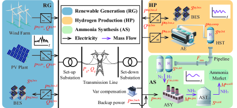
II Structure of ReP2A Systems
An off-grid ReP2A system, as presented in Fig. 1, typically encompasses the generation, storage, delivery, and consumption of electricity and hydrogen alongside the production, storage, and sale of ammonia. As discussed in Section I-A, these processes may belong to different stakeholders in real-life projects [9, 10]. The stakeholders trade electricity, hydrogen, and ammonia with one another.
In the complete green ammonia production process, maintaining energy and mass balance is crucial. The RG, HP, and AS exhibit distinct flexibility due to their inherent physical characteristics. To accommodate the heterogeneous flexibility, multi-type buffer systems (BSs) are implemented, with staged BES, HST, and AST designated for different timescales.
Without loss of generality, we make the following assumptions in analyzing the MSSE:
1) The RG, HP, and AS operate under individual rationality, aiming to minimize their own planning and operational costs.
2) Electricity and hydrogen prices are determined by the interaction between stakeholders without any additional constraints. The ammonia price follows the external market.
3) The RG and HP can both invest in their own BES. The HP and AS can both invest in HSTs.
4) The electricity transmission network is owned by the RG, and the hydrogen delivery network is owned by the HP. The network distances are determined by the geographical locations of the RG, HP, and AS.
5) The capacities of wind and solar power are predetermined based on local resources prior to planning.
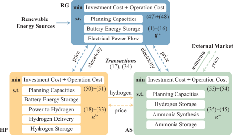
III MSSE Model of the ReP2A System
This section provides a detailed modeling framework for the planning problems of the RG, HP, and AS. Furthermore, we outline the noncooperative game structure of the MSSE model for the ReP2A system.
III-A Modeling the Whole Process of ReP2A
The entire ReP2A process involves the flow of energy and mass related to electricity, hydrogen, and ammonia. The detailed physical models and planning and operational constraints of the corresponding stakeholders are as follows, where 1)–3) pertains to the RG, 5)–8) pertains to the HP, 10)–12) pertains to the AS, and 4) and 9) are the constraints coupling multiple stakeholders.
III-A1 RG Planning Capacities
The equipment to be invested in by the RG includes BES and var compensation (VC) for managing active and reactive power. Their capacities are limited:
| (1) |
III-A2 BES Operation
The BES provides both active and reactive power support. Its charging, discharging, and state of charge (SOC) are constrained by
| (2) | |||
| (3) | |||
| (4) | |||
| (5) | |||
| (6) |
III-A3 Electrical Power Flow
III-A4 Electricity Transactions
The RG stakeholder sells renewable electricity to the HP and AS stakeholders. When a transaction is completed, the quantity and price satisfy:
| (17) |
where and are the dual variables for the individual planning problems of RG/HP/AS, respectively.
III-A5 HP Planning Capacities
The HP can invest in alkaline electrolyzers (AEs), HSTs, and its own BESs, as shown in Fig. 1. The planning capacities of the AE and HST are limited by
| (18) |
and the planning and operational constraints of the BES share the same forms of (1) and (2)–(6), with decision variables replaced by , , , and .
III-A6 P2H Operation
The linear model (19) from [12] is used to approximate the hydrogen production of the industry-scale hydrogen plant. The load range follows (20). Before storage and delivery, hydrogen is pressurized, and the power consumption follows (21). Additionally, the HP stakeholder may also invest in BES to assist in maintaining power balance (22) at the load bus and managing electricity transactions with the RG.
| (19) | |||
| (20) | |||
| (21) | |||
| (22) |
III-A7 HST Operation
III-A8 Hydrogen Delivery Network
The hydrogen flow in pipelines can be modelled by the modified Weymouth equation with second-order cone relaxation [25], as (27)–(29). Linepack dynamics are shown in (30)–(31), and linepack recycling conditions are presented in (32) for each operational horizon. The balance of hydrogen flow in the network is constrained by (33).
| (27) | |||
| (28) | |||
| (29) | |||
| (30) | |||
| (31) | |||
| (32) | |||
| (33) |
III-A9 Hydrogen Transaction
The HP stakeholder sells hydrogen to the AS, and the clearing condition of the transaction is
| (34) |
where are dual variables.
III-A10 AS Planning Capacities
The AS stakeholder may invest in ASY, AST, and its own HST to accommodate the variable hydrogen supply and help bargain with the HP stakeholder. The capacities of these facilities are limited by
| (35) |
III-A11 ASY Operation
The ASY produces ammonia from hydrogen bought from the HP and nitrogen separated from the air via the Haber–Bosch process [4]. Its hydrogen and power consumption (for air separation and other auxiliary equipment) satisfy (36) and (37) [12]. The electrical power comes not only from the RG but also from the backup power supply, as shown in (38), to ensure chemical process safety. The operating range and ramping limits of ASY, constrained by chemical safety considerations [18], are shown in (39)–(40), and the balance of hydrogen is depicted in (41).
| (36) | ||||
| (37) | ||||
| (38) | ||||
| (39) | ||||
| (40) | ||||
| (41) |
III-A12 AST Operation
The AST invested in by the AS is used to accommodate the varying yield of green ammonia and manage the sales to the external ammonia market under fluctuating prices. The operational constraints of the AST include
| (42) | |||
| (43) | |||
| (44) | |||
| (45) |
III-B Multi-Stakeholder Sizing Model
In the planning and operation phases, the RG, HP, and AS stakeholders interact with one another, requiring that the competing economic benefits of each stakeholder be considered, which differs from planning the ReP2A system as a single entity as reported in the literature. To characterize these interactions, a multistakeholder sizing model is proposed. The mathematical expressions are given as follows.
III-B1 RG
The objective of RG planning is to minimize its total cost ,
| (46) |
which includes the investment cost
| (47) |
and the operational cost
| (48) |
where is the capital recovery factor; and are the discount rate and lifetime; is the transmission line cost; and is the annual operation and maintenance (O&M) cost factor.
III-B2 HP
The planning goal of the HP stakeholder is to minimize its total cost
| (49) |
which includes investment cost and operational cost :
| (50) | ||||
| (51) |
where is the hydrogen pipeline cost.
III-B3 AS
The planning goal of the AS stakeholder is to minimize its total cost:
| (52) |
where the investment cost and operation cost follow
| (53) | ||||
| (54) |
Given the above, we summarize the multistakeholder planning problem in Table I. For simplicity, we use and to denote all independent decision variables and constraints of the RG, HP, and AS.
Considering the individual rationality of each stakeholder and competition in the transactions, we frame the multi-stakeholder sizing problem as a non-cooperative game and propose an MSSE model for the ReP2A system, with the game structure depicted in Fig. 2. According to (46)-(54), there are conflicts of interest among RG, HP, and AS, particularly in terms of the revenues and costs related to electricity and hydrogen trading, which will be discussed in Section 10. Moreover, the investment costs of each stakeholder are not balanced due to heterogeneous physical characteristics in the staged processes, and we discuss this later in Sections V-C and V-D.
IV Solution Method for the MSSE Model
To obtain the equilibrium of the proposed MSSE model, this section transforms the system of equations for solving equilibrium, using the direct approach, into a convex optimization problem. A temporal decomposition-based algorithm is subsequently developed to solve this problem efficiently.
IV-A Direct Approach Based on KKT Conditions
The equilibrium of noncooperative games is usually solved via fixed-point iteration [26] and direct approaches [27, 22], including those based on Karush–Kuhn–Tucker (KKT) conditions [27] and strong duality [22]. However, the fixed-point iteration approach cannot ensure convergence, and strong duality introduces bilinear terms, making it challenging to solve. Thus, we attempt to solve the MSSE model via KKT conditions.
The RG, HP, and AS models established in Section III are all convex. The KKT conditions for each stakeholder are given as follows:
| (55a) | |||
| (55b) | |||
| (55c) | |||
where is the dual variable of .
The solution of the joint KKT conditions is the equilibrium [28]. However, dealing with the complementary constraints (55b) in introduces many 0–1 variables when applied to complex problems, making them difficult to solve. Therefore, we construct an equivalent optimization problem [29, 30], formed as second-order cone programming (SOCP), to address the joint KKT conditions.
IV-B Equivalent Problem for Solving the Equilibrium
The dual variables (17) and (34) represent the equilibrium prices for different stakeholders. When transactions are reached, trading prices w.r.t. all parties are the same, as
| (56) |
The equilibrium under constraint (56) is known as variational equilibrium (VE) [22].
Proof.
The nonconvex terms in the original expression of the objective of (57) include , , and . Substituting (17), (34), and (56) into these nonconvex terms yields zero, indicating that the objective of (57) is substantially linear. Hence, problem (57) is convex. Its optimality follows the KKT conditions:
| (58a) | |||
| (58b) | |||
| (58c) | |||
| (58d) | |||
where is the Lagrangian of (57); (58b) are derived similarly to (58), with the detailed expressions not given here due to space limitations; , , and are all zero. As a result, (58) can be reformulated as:
| (59a) | |||
| (59b) | |||
In this way, we can solve an SOCP to obtain the equilibrium rather than the nonconvex system of equations .
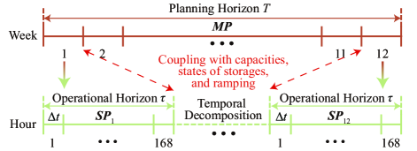
IV-C Temporal Decomposition-Based Solution Algorithm
The proposed multistakeholder planning problem involves ASY and AST, thus requiring attention to long-term power and mass balance due to their slow dynamics [12]. Therefore, the classical power system planning paradigms based on typical days are no longer applicable here. To address the issues of long-term balance, we consider a consecutive operational horizon composed of 12 typical weeks selected from 12 months.
When considering an operational horizon of 12 weeks with a step length of 1 hour, there are 274,200 constraints and 175,403 variables. Although the equivalent MSSE problem (57) is an SOCP, which is typically considered easy to solve, it is challenging to solve in this case because of its high dimensionality.
Fortunately, the horizon can be divided into several consecutive horizons of length with only a few temporally coupled constraints, such as the states of the HST and AST and the ramping of the ASY. Consequently, (57) can be decomposed into a planning master problem (MP) and 12 operational subproblems (SPs), as illustrated in Fig. 3, which are easy to solve via the GBD.
Furthermore, the MP is a simple linear programming (LP). In GBD, adding multiple cuts, even if some are ineffective, almost does not slow down the solution of MP but rather accelerates the convergence compared to adding a single effective cut. Hence, we solve it using multi-cut GBD and parallelize the SPs to speed up the solving process.
For easy understanding, problem (57) is rewritten as follows:
| (60a) | ||||
| s.t. | (60b) | |||
| (60c) | ||||
where comprises the planning capacities and operational variables related to slow dynamics, including , and ; are all operational variables w.r.t. the th week; their feasible sets are and , respectively; , , , , and are the coefficient matrices; (60c) are the coupling constraints involving ① operational variables constrained by planning capacities in SPs; and ② the states of HST, AST, and ramping of ASY between adjacent SPs. The overall procedure of solving the MSSE via multicut GBD is summarized as follows.
Step 0: Initialize , the iteration index , and the convergence tolerance ; set the initial upper bound UB and lower bound LB of the objective (60a).
Step 1: Solve the 12 parallelized SPs with fixed , with , as
| s.t. | ||||
| (61) |
Step 1a: If the th SP is feasible, obtain the optimal solution and dual variables , and generate the optimal cut, as
| (62) |
Step 1b: If the th SP is infeasible, construct a relaxed SP:
| s.t. | ||||
| (63) |
where is the introduced relaxation vector. Solve the relaxed SP (63) to obtain the optimal solution and dual variable and generate a feasible cut
| (64) |
Step 1c: If all the SPs are feasible, then update the upper bound .
Step 2: Update by solving the MP
| s.t. | ||||
| (65) |
where is the lower bound of the augmented Lagrangian of the -th SP. Then, update .
Step 3: If , output the obtained optimum; otherwise, update and return to Step 1.
V Case Studies
V-A Case Setups
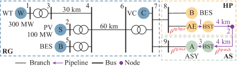
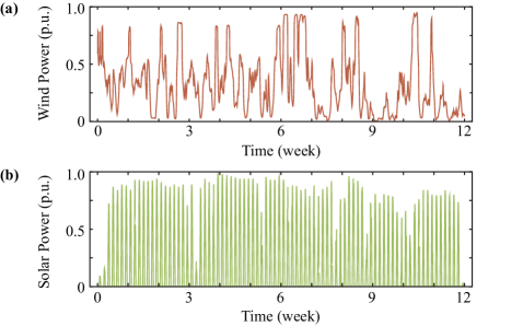
We analyze the MSSE of an off-grid ReP2A system based on a real-life project in North China, as shown in Fig. 4. The system includes a 300-MW wind farm and a 100-MW photovoltaic (PV) array. Wind and solar data from 12 typical weeks, selected from historical records [7], as shown in Fig. 5. Their FLHs are about 3,033 and 1,808 hours, respectively. The external ammonia price is based on the historical market price of fossil fuel-based ammonia [11]. Key investment and operation parameters are detailed in Tables III and III, respectively.
| Facility | Unit investment cost | Lifetime (years) |
|---|---|---|
| WT | 5,000 CNY/kW | 20 |
| PV | 4,000 CNY/kW | 20 |
| BES | 1,500 CNY/kWh | 20 |
| VC | 200 CNY/kVar | 15 |
| AE | 3,500 CNY/kW | 10 |
| HST | 250 CNY/Nm3 | 20 |
| ASY | 21,706 CNY/(t/h) | 20 |
| AST | 3300 CNY/t | 20 |
| Transmission line | 2,000,000 CNY/km | 40 |
| Hydrogen pipeline | 4,000,000 CNY/km | 40 |
The simulations are performed via Wolfram Mathematica 14.0 on a desktop with an Intel Core i5-12400@2.5 GHz CPU and 16 GB of RAM. The MP and SPs in the temporal decomposition-based algorithm are solved via Gurobi 11.0 and Mosek 10.1, respectively. The convergence tolerance is set at 10-4. The overall solving time is approximately 40 minutes.
To account for the interests of the three stakeholders, we define the average transaction prices of electricity and hydrogen , , and as
| (66) | ||||
| (67) | ||||
| (68) |
Furthermore, we use the LCOA to evaluate the overall technoeconomic performance of the ReP2A system as follows:

V-B Analysis of Typical Operational and Trading Results under Equilibrium in the Base Case
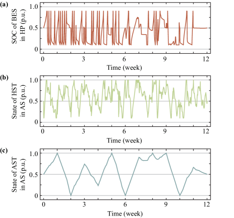
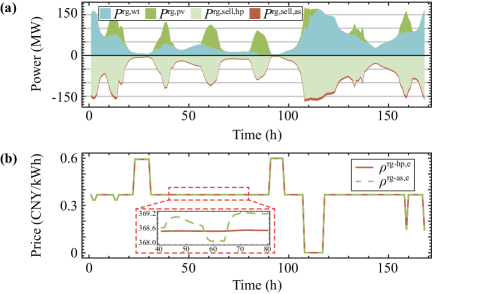
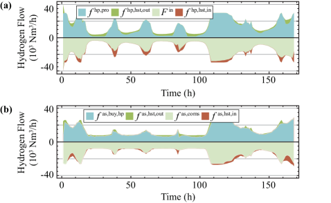
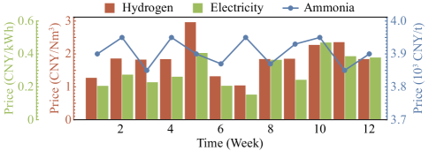
We analyze the operational behaviors of the staged BSs and conduct a base-case equilibrium analysis. The planning result obtained by the MSSE model is: MWh, MVar, MW, Nm3, t/h, and t, as listed in Table IV, labeled as C1. The LCOA composition is shown in Fig. 6. Fig. 7 illustrates the states of BES in HP, HST in AS, and AST in AS throughout the planning horizon. The state of the BES in RG and the state of the HST in HP are not listed here due to the space limit. Fig. 9(a) shows the wind and solar power and loads of AE and ASY in the 8th week, with the electricity prices presented in Fig. 9(b). Fig. 9 illustrates the hydrogen flow balance at the HP and AS nodes. Fig. 10 shows the average electricity and hydrogen prices of AS and the ammonia price each week.
As shown in Fig. 7, the fluctuating patterns of the BES, HST, and AST are daily, weekly, and cross-weekly, respectively, each suited to different time scales. The states of the BES and HST fluctuate with wind and solar power, while the state of the AST follows the opposite trend of the ammonia price, as shown in Fig. 10, reflecting its profit-chasing behavior.
Fig. 9 shows that peak, flat, and valley periods of wind and solar power correspond to low, medium, and high electricity prices under equilibrium, such as h, h, and h, respectively. During flat periods, the prices stabilize around CNY/kWh. Microscopically, depends more on wind and solar resources compared to due to the smaller invested capacity of the RG-side BES. During high periods, the electricity price approaches CNY/kWh due to the saturated production capacities of AE and ASY, causing the renewable power supply to exceed the demand. During low periods, the prices stay around CNY/kWh, as it is enveloped by the backup power price ( CNY/kWh) for the ASY.
Combining Figs. 7 and 9, we observe that the fluctuations of renewable generation, hydrogen production, and hydrogen consumption (i.e., ASY) are progressively buffered by the staged BESs and HSTs. The hydrogen trading quantities follow the electricity trading. Further examining Fig. 10, we can find that the trend of the hydrogen prices is highly consistent with the electricity prices and shows some consistency with the external ammonia price. Since wind and solar resources are negatively correlated with electricity prices, we infer a negative correlation between the renewables and the equilibrium hydrogen price.
Moreover, we can conclude that the cost of green ammonia, influenced by the electricity and hydrogen prices, is significantly affected by the uncertainty of wind and solar resources. This may pose risks to both the producers and consumers in the green ammonia market. To further enhance the competitiveness of green ammonia, improving trading mechanisms by introducing spot markets [25] or financial tools [11, 33] is recommended.
| Case |
|
|
|
|
|
||||||||||||||
|---|---|---|---|---|---|---|---|---|---|---|---|---|---|---|---|---|---|---|---|
| C1 | {7.29, 0.01, 77.13, 149.13, 52.00103, 72.42103, 13.10, 2430.76} | {–11.60, 5.35, –24.15} | –30.40 | 4298.5 | {0.2288, 0.2445, 1.765} | ||||||||||||||
| C2 | {0, 0.05, 84.55, 149.29, 48.35103, 77.82103, 13.08, 2427.59} | {–36.89, –3.35, 9.84} | –30.40 | 4298.3 | {0.1983, 0.2181, 1.568} | ||||||||||||||
| C3 | {85.67, 0.11, 0, 150.62, 45.21103, 92.91103, 13.08, 2410.34} | {–25.03, 1,69, –7.14} | –30.48 | 4299.1 | {0.2298, 0.2305, 1.665} | ||||||||||||||
| C4 | {14.75, 0.02, 70.18, 149.754, 0, 130.34103, 13.17, 2419.91} | {–21.53, 23.80, –32.83} | –30.83 | 4303.7 | {0.2187, 0.2368, 1.810} | ||||||||||||||
| C5 | {12.52, 0.19, 73.18, 150.74, 130.65103, 0, 13.22, 2425.50} | {–38.70, 5.73, 2.32} | –30.98 | 4301.0 | {0.1983, 0.2152, 1.625} | ||||||||||||||
| C6 | {85.44, 0.01, 0, 150.33, 131.32103, 0, 13.19, 2426.35} | {–38.30, 24.31, –16.75} | –30.74 | 4302.2 | {0.2139, 0.2314, 1.735} | ||||||||||||||
| C7 |
|
{–4.29, 36.28, –68.97} | –36.98 | 4348.7 | {0.2377, 0.2407, 1.987} | ||||||||||||||
| C8 |
|
{–111.69, 92.84, –66.03} | –84.88 | 5108.5 | {0.1761, 0.1619, 2.020} | ||||||||||||||
| D1 | {28.59, 0.06, 62.26, 157.22, 61.36103, 83.25103, 13.58, 2380.3} | {6.34, 14.96, –17.90} | 3.40 | 4292.6 | {0.2476, 0.2711, 1.913} | ||||||||||||||
| D2 | {0, 0.02, 90.83, 157.22, 67.53103, 78.18103, 13.58, 2384.6} | {–5.27, 0.66, 8.01} | 3.40 | 4293.6 | {0.2289, 0.2510, 1.767} | ||||||||||||||
| D3 | {90.99, 0.04, 0, 157.31, 65.89103, 81.99103, 13.57, 2383.9} | {–6.26, 11.63, –2.05} | 3.32 | 4293.6 | {0.2466, 0.2610, 1.823} | ||||||||||||||
| D4 | {13.01, 0.02, 73.10, 151.23, 0, 136.41103, 13.28, 2412.5} | {11.42, 9.22, –18.03} | 2.61 | 4298.3 | {0.2557, 0.2545, 1.914} | ||||||||||||||
| D5 | {30.34, 0.00, 61.02, 157.83, 153.75103, 0, 13.57, 2383.9} | {7.23, 10.56, –14.65} | 3.14 | 4296.0 | {0.2491, 0.2620, 1.908} | ||||||||||||||
| D6 | {91.50, 0.04, 0, 157.31, 152.46103, 0, 13.66, 2380.3} | {–17.64, 10.03, 10.68} | 3.07 | 4296.8 | {0.2339, 0.2452, 1.763} | ||||||||||||||
| E1 | {28.59, 0.06, 62.26, 157.22, 61.36103, 83.25103, 13.58, 2380.3} | {0.05, 1.82, 1.53} | 3.40 | 4292.6 | {0.2476, 0.2711, 1.913} |
V-C Planning Results for the Multistakeholder Sizing Equilibrium under Different Configurations
We further analyze the MSSE under eight cases to reveal a potential dilemma in multistakeholder investment practices during implementation of ReP2A systems:
- •
-
•
C2: The RG is not allowed to configure BES ().
-
•
C3: The HP is not allowed to configure BES ().
-
•
C4: The HP is not allowed to configure HST ().
-
•
C5: The AS is not allowed to configure HST ().
-
•
C6: The HP is not allowed to configure BES, and the AS is not permitted to configure HSTs (, ).
-
•
C7: The WT and PV capacities are not fixed, i.e., and are to be optimized, and the capacity of ASY is fixed at t/h, as in [7]. The other settings are consistent with C1.
- •
Table IV shows the planning results and operational performance. In the base case (C1), the AS has the highest cost among the three stakeholders, with almost all profits transferred to the HP, which aligns with the AS’s reluctance to participate in a demo ReP2A project in North China. Comparing C1 and C2, we can see that the investment in BES by the RG can significantly increase electricity prices, as explained in Section V-B and Fig. 9. Therefore, the current policies requiring integrated investment in wind and solar power and BES benefit the interests of the RG in implementing ReP2A projects. Further analysis of C1 and C3 reveals that investing in the BES by the HP also increases its benefits by increasing flexibility in response to fluctuations in wind, solar, and electricity prices.
In case C7, where the ASY capacity is predetermined on the basis of ammonia demand, the overall technoeconomic viability of ReP2A is inferior to that in cases C1 to C6. This suggests that sizing on the basis of wind and solar resources is marginally more advantageous than sizing by ammonia demand. In C8, with all facilities’ capacities fixed, the overall technoeconomic viability of ReP2A becomes unoptimistic, and significant differences in stakeholders’ interests can be observed. Therefore, we observe that coordinated sizing for renewable, AE, and ASY facilities, although conducted by stakeholders with conflicting interests, contributes to the technoeconomic viability of ReP2A.
In summary, for cases C1 to C6, to improve the overall technoeconomic performance of the ReP2A system, the capacities of renewables, AE, ASY, and BSs must be properly aligned. However, despite efforts to optimize BES and HST configurations, stakeholders’ interests remain unbalanced due to their heterogeneous characteristics. Specifically, in no case do all three stakeholders achieve a positive profit. This phenomenon is very different from the well-studied applications in power systems, for example, games among power sources [20], microgrids [21], and prosumers [30]. Analyzing the the HP’s cost in C1 to C6, we can see that the HP plays a dominant role in the equilibrium. To make ReP2A projects invested in by multiple stakeholders implementable, benefit transfer mechanisms or pricing agreements could be established before implementing a ReP2A project to ensure the interests of all parties.
V-D Recommendation for the Investment of ReP2A Projects
According to the results from C1 to C6, at least one stakeholder will incur a loss, thus diminishing the overall motivation for investment. To address this issue, providing subsidies [34, 14] for green ammonia could increase economic competitiveness and stimulate the growth of the green ammonia industries. To explore this, we introduce six additional cases, denoted as D1 to D6, where the ammonia price is increased by 400 CNY/t while other settings remain the same as those in C1–C6. The simulation results are shown in Table IV.
In cases D1 to D6, although social welfare is positive, no one achieves mutual benefits under equilibrium, which is consistent with the findings from C1 to C6. Therefore, we conclude that the multistakeholder ReP2A system can hardly achieve reasonable investment under free competition. To address this, it is recommended that regulatory authorities establish a negotiation platform for multistakeholder investment. This would allow stakeholders to form a consortium [7] and enter into benefit transfer or pricing agreements that ensure mutual benefits and facilitate successfully implementing ReP2A projects.
As an example, in case D1, RG and HP are profitable, whereas AS incurs a loss. To mitigate this, we propose a benefit transfer mechanism whereby RG transfers 3% of its revenue from electricity sales to the HP and where the HP transfers 6% of its revenue from hydrogen sales to the AS. The simulation results for this scenario, denoted as E1, are recorded in Table IV, which shows that all three stakeholders achieve a positive profit. Due to the space limit, we will not discuss this further.
VI Conclusions
This study proposes a multistakeholder sizing equilibrium (MSSE) model for planning an ReP2A system, encompassing the entire process of generation, storage, and utilization of electricity, hydrogen, and ammonia. A multicut generalized Bender decomposition (GBD) approach is developed to efficiently address long-term energy and mass balancing problems. The following findings are drawn from the simulation results.
1) The interests of RG, HP, and AS stakeholders are not balanced due to their heterogeneous flexibility. They cannot simultaneously achieve positive profit under free competition, causing at least one stakeholder to be reluctant to invest, thereby making the ReP2A project unimplementable.
2) To increase the attractiveness and feasibility of ReP2A projects, regulators should establish a negotiation platform where stakeholders can sign benefit transfer or pricing agreements, enabling mutual benefits and ensuring the successful implementation of ReP2A projects.
Future research will focus on the uncertainties associated with renewable resources and external ammonia prices. Additionally, the equilibrium in ammonia transactions with external chemical users within the ReP2A system will be considered.
References
- [1] X. Yang, C. P. Nielsen, S. Song, and M. B. McElroy, “Breaking the hard-to-abate bottleneck in China’s path to carbon neutrality with clean hydrogen,” Nat. Energy, vol. 7, no. 10, pp. 955–965, Sep. 2022.
- [2] D. R. MacFarlane, P. V. Cherepanov, J. Choi, B. H. Suryanto, R. Y. Hodgetts, J. M. Bakker, F. M. F. Vallana, and A. N. Simonov, “A roadmap to the ammonia economy,” Joule, vol. 4, no. 6, pp. 1186–1205, Jun. 2020.
- [3] The Energy Bureau of Inner Mongolia Autonomous Region, “Notice of Inner Mongolia Autonomous Region Energy Bureau on carrying out the 2022 wind-solar hydrogen production integration demonstration.” [Online]. Available: http://dbnyb.com/07/taiyangnen/2021/0827/51472.html
- [4] N. Campion, H. Nami, P. R. Swisher, P. V. Hendriksen, and M. Münster, “Techno-economic assessment of green ammonia production with different wind and solar potentials,” Renew. Sustain. Energy Rev., vol. 173, p. 113057, Mar. 2023.
- [5] National Development and Reform Commission, “Natural Gas Utilization Management Measures.” [Online]. Available: https://www.ndrc.gov.cn/xxgk/zcfb/fzggwl/202406/t20240619_1387036.html
- [6] Z. Yu, J. Lin, F. Liu, J. Li, Y. Zhao, and Y. Song, “Optimal sizing of isolated renewable power systems with ammonia synthesis: Model and solution approach,” IEEE Trans. Power Syst., pp. 1–14, 2024.
- [7] Z. Yu, J. Lin, F. Liu, J. Li, Y. Zhao, Y. Song, Y. Song, and X. Zhang, “Optimal sizing and pricing of grid-connected renewable power to ammonia systems considering the limited flexibility of ammonia synthesis,” IEEE Trans. Power Syst., vol. 39, no. 2, pp. 3631–3648, Mar. 2024.
- [8] R. M. Nayak-Luke and R. Bañares-Alcántara, “Techno-economic viability of islanded green ammonia as a carbon-free energy vector and as a substitute for conventional production,” Energy Environ. Sci., vol. 13, no. 9, pp. 2957–2966, Sep. 2020.
- [9] R. Fernández-González, F. Puime-Guillén, and M. Panait, “Multilevel governance, PV solar energy, and entrepreneurship: The generation of green hydrogen as a fuel of renewable origin,” Util. Pol., vol. 79, p. 101438, Dec. 2022.
- [10] National Coal Chemicals Website, “Investment of 3 billion RMB, Chongqing’s 200,000-ton synthetic ammonia unit achieves another important milestone, scheduled to be completed and put into operation by the end of 2021.” [Online]. Available: http://www.coalchem.org.cn/news/html/800201/188978.html
- [11] S. Wu, J. Lin, J. Li, F. Liu, Y. Song, Y. Xu, X. Cheng, and Z. Yu, “Multi-timescale trading strategy for renewable power to ammonia virtual power plant in the electricity, hydrogen, and ammonia markets,” IEEE Trans. Energy Mark. Policy Regul., vol. 1, no. 4, pp. 322–335, Dec. 2023.
- [12] J. Li, J. Lin, P.-M. Heuser, H. U. Heinrichs, J. Xiao, F. Liu, M. Robinius, Y. Song, and D. Stolten, “Co-planning of regional wind resources-based ammonia industry and the electric network: A case study of Inner Mongolia,” IEEE Trans. Power Syst., vol. 37, no. 1, pp. 65–80, Jan. 2022.
- [13] H. Zhao, L. M. Kamp, and Z. Lukszo, “Exploring supply chain design and expansion planning of China’s green ammonia production with an optimization-based simulation approach,” Int. J. Hydrogen Energy, vol. 46, no. 64, pp. 32 331–32 349, Sep. 2021.
- [14] H. Zhao, L. M. Kamp, and Z. Lukszo, “The potential of green ammonia production to reduce renewable power curtailment and encourage the energy transition in China,” Int. J. Hydrogen Energy, vol. 47, no. 44, pp. 18 935–18 954, May 2022.
- [15] Q. V. Dinh, P. H. T. Pereira, A. J. Nagle, P. G. Leahy et al., “Levelised cost of transmission comparison for green hydrogen and ammonia in new-build offshore energy infrastructure: Pipelines, tankers, and HVDC,” Int. J. Hydrogen Energy, vol. 62, pp. 684–698, Apr. 2024.
- [16] F. Zhao, Y. Li, X. Zhou, D. Wang, Y. Wei, and F. Li, “Co-optimization of decarbonized operation of coal-fired power plants and seasonal storage based on green ammonia co-firing,” Appl. Energy, vol. 341, p. 121140, Jul. 2023.
- [17] J. Ikäheimo, J. Kiviluoma, R. Weiss, and H. Holttinen, “Power-to-ammonia in future north european 100% renewable power and heat system,” Int. J. Hydrogen Energy, vol. 43, no. 36, pp. 17 295–17 308, Sep. 2018.
- [18] S. Klyapovskiy, Y. Zheng, S. You, and H. W. Bindner, “Optimal operation of the hydrogen-based energy management system with P2X demand response and ammonia plant,” Appl. Energy, vol. 304, p. 117559, Dec. 2021.
- [19] O. Osman, S. Sgouridis, and A. Sleptchenko, “Scaling the production of renewable ammonia: A techno-economic optimization applied in regions with high insolation,” J. cleaner prod., vol. 271, p. 121627, Oct. 2020.
- [20] C. Ruiz, A. J. Conejo, and Y. Smeers, “Equilibria in an oligopolistic electricity pool with stepwise offer curves,” IEEE Trans. Power Syst., vol. 27, no. 2, pp. 752–761, May 2012.
- [21] A. Naebi, S. SeyedShenava, J. Contreras, C. Ruiz, and A. Akbarimajd, “EPEC approach for finding optimal day-ahead bidding strategy equilibria of multi-microgrids in active distribution networks,” Int. J. Electr. Power Energy Syst., vol. 117, p. 105702, May 2020.
- [22] S. Chen, A. J. Conejo, and Z. Wei, “Conjectural-variations equilibria in electricity, natural-gas, and carbon-emission markets,” IEEE Trans. Power Syst., vol. 36, no. 5, pp. 4161–4171, Sep. 2021.
- [23] Q. Wang, W. Wu, C. Lin, S. Xu, S. Wang, and J. Tian, “An exact relaxation method for complementarity constraints of energy storages in power grid optimization problems,” Appl. Energy, vol. 371, p. 123592, 2024.
- [24] M. Farivar and S. H. Low, “Branch flow model: Relaxations and convexification—Part I,” IEEE Trans. Power Syst., vol. 28, no. 3, pp. 2554–2564, Aug. 2013.
- [25] Q. An, G. Li, X. Fang, F. Li, and J. Wang, “On the decomposition of locational marginal hydrogen pricing—Part II: Solution approach and numerical results,” IEEE Trans. Ind. Inf., pp. 1–11, 2024.
- [26] H. Li, Z. Ren, A. Trivedi, P. P. Verma, D. Srinivasan, and W. Li, “A noncooperative game-based approach for microgrid planning considering existing interconnected and clustered microgrids on an island,” IEEE Trans. Sustain. Energy, vol. 13, no. 4, pp. 2064–2078, Oct. 2022.
- [27] G. Pan, W. Gu, S. Chen, Y. Lu, S. Zhou, and Z. Wei, “Investment equilibrium of an integrated multi–stakeholder electricity–gas–hydrogen system,” Renew. Sustain. Energy Rev., vol. 150, p. 111407, Oct. 2021.
- [28] A. Dreves, F. Facchinei, C. Kanzow, and S. Sagratella, “On the solution of the KKT conditions of generalized nash equilibrium problems,” SIAM J. Optim., vol. 21, no. 3, pp. 1082–1108, Sep. 2011.
- [29] R. Egging-Bratseth, T. Baltensperger, and A. Tomasgard, “Solving oligopolistic equilibrium problems with convex optimization,” Eur. J. Oper. Res., vol. 284, no. 1, pp. 44–52, Jul. 2020.
- [30] Z. Wang, F. Liu, Z. Ma, Y. Chen, M. Jia, W. Wei, and Q. Wu, “Distributed generalized nash equilibrium seeking for energy sharing games in prosumers,” IEEE Trans. Power Syst., vol. 36, no. 5, pp. 3973–3986, Sep. 2021.
- [31] A. M. Geoffrion, “Generalized benders decomposition,” J. Optim. Theory Appl., vol. 10, pp. 237–260, Oct. 1972.
- [32] J. R. Birge and F. V. Louveaux, “A multicut algorithm for two-stage stochastic linear programs,” Eur. J. Oper. Res., vol. 34, no. 3, pp. 384–392, Mar. 1988.
- [33] Y. Cai, Y. Qiu, B. Zhou, T. Zang, G. He, and X. Ji, “Green ammonia futures: Design and analysis based on general equilibrium theory,” in 2023 IEEE Sustain. Power and Energy Conf. (iSPEC), 2023, pp. 1–6.
- [34] C. A. Del Pozo and S. Cloete, “Techno-economic assessment of blue and green ammonia as energy carriers in a low-carbon future,” Energy Convers. Manage., vol. 255, p. 115312, Mar. 2022.