Temporal Reversed Training for Spiking Neural Networks with Generalized Spatio-Temporal Representation

Abstract

Spiking neural networks (SNNs) have received widespread attention as an ultra-low energy computing paradigm. Recent studies have focused on improving the feature extraction capability of SNNs, but they suffer from inefficient inference and suboptimal performance. In this paper, we propose a simple yet effective temporal reversed training (TRT) method to optimize the spatio-temporal performance of SNNs and circumvent these problems. We perturb the input temporal data by temporal reversal, prompting the SNN to produce original-reversed consistent output logits and to learn perturbation-invariant representations. For static data without temporal dimension, we generalize this strategy by exploiting the inherent temporal property of spiking neurons for spike feature temporal reversal. In addition, we utilize the lightweight “star operation” (element-wise multiplication) to hybridize the original and temporally reversed spike firing rates and expand the implicit dimensions, which serves as spatio-temporal regularization to further enhance the generalization of the SNN. Our method involves only an additional temporal reversal operation and element-wise multiplication during training, thus incurring negligible training overhead and not affecting the inference efficiency at all. Extensive experiments on static/neuromorphic object/action recognition, and 3D point cloud classification tasks demonstrate the effectiveness and generalizability of our method. In particular, with only two timesteps, our method achieves 74.77% and 90.57% accuracy on ImageNet and ModelNet40, respectively.

Introduction

Recently, brain-inspired spiking neural networks (SNNs) have received widespread attention. Unlike traditional artificial neural networks (ANNs), which transfer information using intensive floating-point values, SNNs transfer discrete 0-1 spikes between neurons, providing a more efficient neuromorphic computing paradigm (Yao et al. 2023). In addition, spiking neurons, which simulate the dynamics of biological neurons over multiple timesteps, can effectively extract temporal features (Kim et al. 2023). These superior properties have led to the application of SNNs to a variety of spatio-temporal tasks such as object recognition, detection, generation, and natural language processing (Su et al. 2023; Kamata, Mukuta, and Harada 2022; Bal and Sengupta 2024).

To improve the performance of SNNs, researchers have made considerable efforts to enhance their feature extraction ability. For instance, the temporal properties of SNNs are optimized through heterogeneous timescales (Chakraborty et al. 2024), batch normalization (BN) methods adapted to the temporal dimension (Duan et al. 2022; Jiang et al. 2024b), and improved neuron dynamics (Ponghiran and Roy 2022). Alternatively, the spatial properties of SNNs are continuously improved with sophisticated network architectures (Yao et al. 2023). However, glory comes with remaining problem that these methods introduce additional computational complexity and negatively affect the inference efficiency. Although there exist alternative methods that only optimize the training process without affecting inference, the performance of these methods is too limited to unleash the full potential of SNNs (Zhang et al. 2024; Zuo et al. 2024). Therefore, how to maximize the spatio-temporal performance of SNNs without compromising the efficiency is an ongoing issue that still deserves attention.

In this paper, we propose a simple yet effective temporal reversed training (TRT) method to improve the spatio-temporal performance of SNNs. We perturbed the SNN during training, pushing it to be immune to these perturbations and to focus on generalizable features. Specifically, for the temporal task, we propose to perturb the inputs with temporal reversal. During training, the SNN simultaneously takes both original and reversed inputs and generates the corresponding pair of outputs. We encourage this pair of outputs to be as similar as possible, allowing the SNN to learn time-invariant generalized spatial representations on the one hand, and perturbation-insensitive stable temporal representations on the other hand. For static tasks without temporal concepts, we utilize the inherent temporal properties of spiking neurons to reverse the encoded temporal spikes to generate the corresponding output pairs. This makes our method simple and versatile in a variety of task scenarios. The perturbation occurs only during training without any additional inference overhead. At first glance, our method bears some resemblance to siamese learning, where different transformed data are fed into an ANN to produce consistent representations (Chen and He 2021; Wang et al. 2022). However, siamese learning relies on complicated data augmentation strategies, whereas our method is more straightforward and versatile by exploiting the inherent temporal properties of SNNs. From another perspective, the process of continuously seeking consistency between the original and temporally reversed outputs can be viewed as distillation learning (Hinton, Vinyals, and Dean 2015), which further supports the performance advantages of our method.

Moreover, we employ the lightweight “star operation” (element-wise multiplication) to hybridize the high-dimensional original and temporally reversed features, expanding the implicit dimensions and prompting the SNN to make correct predictions for the hybrid features. The hybridization further perturbs the temporal dimension and disrupts the spatial feature map, which can be considered as a regularization of high-dimensional features (visualization in Appendix D), allowing the SNN to learn latent representations that are insensitive to spatio-temporal perturbations, thus improving its generalization ability. However, direct “star” hybridization of binary spikes would result in severe information loss. To alleviate this problem, we convert discrete spikes to spike firing rate with a value range of $[0,1]$ and perform spike firing rate “star” hybridization. In this way, we can enhance the performance of the model with only a negligible multiplication overhead during training.

To confirm the effectiveness of our method, we conducted extensive experiments using VGG, ResNet, Transformer, and PointNet architectures on static object recognition, neuromorphic object/action recognition, and 3D point cloud classification tasks. The experimental results show that our method achieves consistent performance gains across these tasks, datasets, and model architectures, with excellent generalizability. In summary, our contributions are as follows:

• We propose to temporally reverse the input/spike features and prompt the SNN to produce consistent outputs to enhance its spatio-temporal feature extraction capability.

• We propose to hybridize high-dimensional original and reversed features with a simple “star operation” to enable the SNN to learn generalized spatio-temporal features.

• Extensive experiments on static/neuromorphic object/action recognition and 3D point cloud classification confirm the effectiveness and versatility of our method. Compared to existing methods, our method exhibits better performance without compromising inference.

Related Work

Spiking Neural Network. To train high-performance SNNs, indirect training based on ANN-to-SNN conversion (Wu et al. 2022; Hao et al. 2023) and direct training method based on surrogate gradient (Wu et al. 2018; Guo et al. 2024; Qiu et al. 2024) have achieved remarkable results. In addition, improved BN strategies (Duan et al. 2022; Jiang et al. 2024b), neuron dynamics (Ponghiran and Roy 2022; Ding et al. 2023; Wang and Yu 2024), and sophisticated architectures borrowed from ANNs (Yao et al. 2023; Li et al. 2024) further boost the performance of SNNs. However, these methods entail additional inference overhead that undermines the central energy advantage of SNNs. Some methods only modify the training of the SNN, preserving low-energy inference (Zhang et al. 2024; Zuo et al. 2024). However, the performance of these methods is still suboptimal, so further exploration of efficient and high-performance SNNs is still necessary. Compared to existing methods, our method is simple, effective, and architecture- and task-agnostic, with superior generalizability.

Siamese Learning. For a given input, siamese learning uses data augmentation to transform it into two different views and increase the similarity between the outputs generated by the two (Chen and He 2021; Wang et al. 2022). This can facilitate the neural network to learn consistent features that are invariant to data transformations. However, this method is extremely sensitive to data augmentation strategies. For our method, we avoid the tedious process of data augmentation search and use the inherent temporal property of SNNs and temporal data for perturbation to improve model performance. From another perspective, our method can be seen as an extension of siamese learning in SNNs, exploiting in particular their inherent temporal properties.

Knowledgw Distillation. Our method pushes the original and temporally reversed outputs of the SNN to be as similar as possible, which can be considered as a knowledge distillation strategy (Hinton, Vinyals, and Dean 2015). Unlike traditional distillation, we utilize temporal properties to allow a single SNN to output both “teacher” and “student” signals, similar to self-distilling learning in ANNs (Zhang et al. 2019; Yuan et al. 2020). The perturbation-free original ouput continuously guides the temporally reversed ouput, driving our SNN to learn perturbation-invariant features, which underpins the performance advantage of our method.

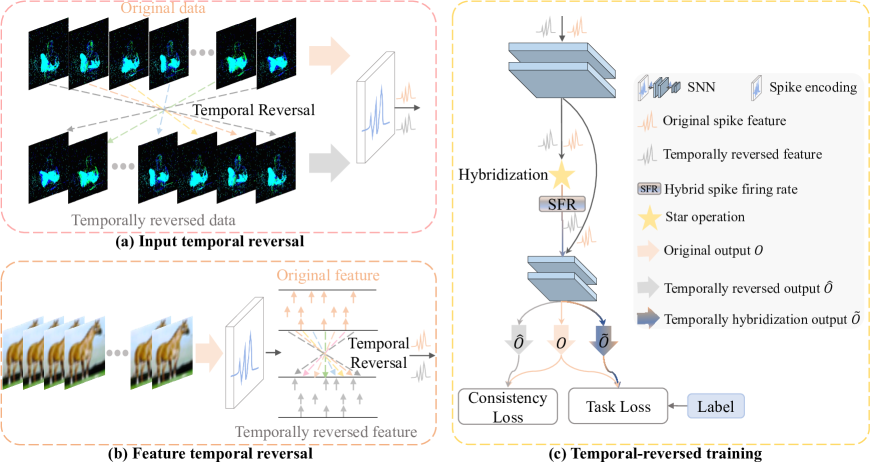
Figure 1: Overview of the TRT method. TRT perturbs temporal and static data by (a) input and (b) feature temporal reversal, allowing the SNN to produce original and temporally reversed outputs, and (c) encouraging both outputs to be as similar as possible to learn generalized perturbation-invariant representations. In addition, TRT hybridizes the original and temporally reversed spike firing rates and expands the implicit dimensionality with a lightweight “star operation”, which can be regarded as a spatio-temporal regularization, further facilitating the generalization of the SNN. TRT introduces only negligible training overhead (temporal reversal and “star operation”) and does not affect the inference efficiency of the SNN.

Method

This section first introduces the basic spiking neuron model, and then illustrates how simple temporal reversal and “star operation” induces the SNN to learn generalized spatio-temporal representations. Finally, we provide the detailed training algorithm for the TRT method.

Spiking Neuron Model

Spiking neurons iteratively receive input currents, accumulate in membrane potentials, and generate spikes. For the most commonly used leaky integrate-and-fire (LIF) model (Wu et al. 2018), the dynamics of the accumulating membrane potential can be expressed as:

$$H_{i}^{l}(t)=\left(1-\frac{1}{\tau}\right)H_{i}^{l}(t-1)+I_{i}^{l}(t),$$ (1)

where $H$ and $I$ denote the membrane potential and afferent current, respectively, $l$ and $i$ are the layer and neuron index, $t$ is the timestep, and $\tau$ is the time constant controlling the degree of leakage of membrane potential.

When the membrane potential $H_{i}^{l}(t)$ reaches the firing threshold $\vartheta$, the spiking neuron will generate a spike $S_{i}^{l}(t)$ and reset the membrane potential:

$$S_{i}^{l}(t)=\left\{\begin{array}[]{cl}1,\quad H_{i}^{l}(t)\geq\vartheta\\ 0,\quad H_{i}^{l}(t)<\vartheta\\ \end{array},\right.$$ (2)

$$H_{i}^{l}(t)=H_{i}^{l}(t)-S_{i}^{l}(t)\vartheta.$$ (3)

Since the spike activity is non-differentiable, we replace the spike derivatives with the surrogate gradient during backpropagation to optimize the SNN using the Backpropagation Through Time (BPTT) algorithm. In this paper, we use the rectangular surrogate function:

$$\frac{\partial S_{i}^{l}(t)}{\partial H_{i}^{l}(t)}\approx\frac{\partial h(H_{i}^{l}(t),\vartheta)}{\partial H_{i}^{l}(t)}=\frac{1}{a}\text{sign}(|H_{i}^{l}(t)-\vartheta|<\frac{a}{2}),$$ (4)

where $a$ is set to 1.0 and is a hyperparameter that controls the shape of the surrogate function.

Temporal Reversal Perturbation

In this section we present how to perform temporal reversal perturbation to improve the spatio-temporal performance of SNNs for temporal and static data, respectively.

Input Temporal Reversal. Without loss of generality, we denote the input data with temporal properties as $X=\{x_{1},x_{2},\cdots,x_{T}\}\in\mathbb{R}^{T\times B\times C_{i}\times H_{i}\times W_{i}}$, where $T,B,C_{i},H_{i}$, and $W_{i}$ are the time, batch, input channel, height and width sizes, respectively. Typically, the temporal input $X$ and the temporal dimension of the SNN are aligned, i.e., $x_{t}$ is input to the SNN at timestep $t$ and ultimately produces the output $o_{t}$. In addition to the original input $X$, we use temporal reversal to additionally generate the temporally reversed input $\hat{X}=\{\hat{x}_{1},\hat{x}_{2},\cdots,\hat{x}_{T}\}$ for perturbation. As shown in Fig. 1 (a), this temporal reversal is achieved by simply flipping the temporal index of the input data X, i.e., $\hat{x}_{t}=x_{T+1-t}$, without laboriously selecting data augmentations to generate additional data views as in siamese learning (Chen and He 2021; Wang et al. 2022). At each timestep $t$, $\hat{x}_{t}$ is fed into the SNN to produce the temporally reversed output $\hat{o}_{t}$.

Feature Temporal Reversal. Input temporal reversal can only be used for tasks with inherent temporal properties, such as neuromorphic or video data. To make this temporal reversal to be effective for static tasks without inherent temporal properties, we further propose feature temporal reversal. For static data $x\in\mathbb{R}^{B\times C_{i}\times H_{i}\times W_{i}}$, SNNs typically input data repeatedly at each timestep and encode it as spikes through the first spiking neuron layer. We denote the primary features after spike encoding by $F=\{f_{1},f_{2},\cdots,f_{T}\}\in\mathbb{R}^{T\times B\times C\times H\times W}$, where $f_{t}$ represents the encoded spikes at timestep $t$. With this, we take advantage of the spiking neuron dynamics to transform the static data $x$ into spatio-temporal spikes $F$ with the temporal dimension. We then apply temporal reversal to the spike feature $F$ and obtain the temporally reversed feature $\hat{F}=\{\hat{f}_{1},\hat{f}_{2},\cdots,\hat{f}_{T}\}$, where $\hat{f}_{t}=F_{T+1-t}$, as shown in Fig. 1 (b). The temporal reversed feature $\hat{F}$ is propagated further forward in the SNN to produce the final temporally reversed output $\hat{O}=\{\hat{o}_{1},\hat{o}_{2},\cdots,\hat{o}_{T}\}$.

Perturbation-Invariant Learning. Through input/feature temporal reversal, we can perturb the temporal dimension of the SNN, regardless of whether the input is inherently temporal or not. To motivate the SNN to learn perturbation-invariant spatio-temporal features, we impel the temporal-reversed output $\hat{O}$ to be as similar as possible to the original output $O$. As shown in Fig. 1 (c), we increase the similarity between the two by imposing a consistency loss $\mathcal{L}_{con}$.

We illustrate the consistency loss in detail with a $C$-way classification task. For the outputs $O$ and $\hat{O}$ of the SNN, the corresponding logits are given as:

$$p_{j}=\frac{e^{z_{j}/T_{tem}}}{\sum^{C}_{c=1}{e^{z_{c}/T_{tem}}}},\hat{p}_{j}=\frac{e^{\hat{z}_{j}/T_{tem}}}{\sum^{C}_{c=1}{e^{\hat{z}_{c}/T_{tem}}}},$$ (5)

where $z=\frac{1}{T}\sum^{T}_{t=1}o_{t}$, $\hat{z}=\frac{1}{T}\sum^{T}_{t=1}\hat{o}_{t}$ are the rate-decoded outputs and the subscript $j$ denotes the $j$-th class. $T_{tem}$ is the temperature scaling hyperparameter used to smooth the logit, which is set to 2 in this paper. We use KL divergence to push the logit of the reversed output to be consistent with the logit of the original output:

$$\mathcal{L}_{con}=T^{2}KL(p||\hat{p})=T^{2}\sum^{C}_{j=1}{p_{j}log(\frac{p_{j}}{\hat{p}_{j}})}.$$ (6)

Thus, as the SNN is trained, both task loss (cross-entropy loss $\mathcal{L}_{CE}$) and consistency loss $\mathcal{L}_{con}$ contribute to the optimization of the parameters:

$$\hat{\mathcal{L}}=\mathcal{L}_{CE}(O,Y)+\mathcal{L}_{con}(O,\hat{O}),$$ (7)

where $Y$ is the ground-truth label.

Feature Hybridization Perturbation

To further improve the generalization of the features learned by the SNN, inspired by the regularization strategy (Srivastava et al. 2014), we propose to hybridize original and temporally reversed features for perturbation. The simple “star operation” (element-wise multiplication) can significantly increase the implicit dimensionality of ANN features, and shares a philosophy with kernel functions (Ma et al. 2024; Shawe-Taylor and Cristianini 2004). Therefore, we propose to perturb the original and temporal reversed features in the SNN with the “star operation” to serve as a spatio-temporal regularization of the high-dimensional features. However, due to the binary nature of the spike, the “star operation” does not contribute to dimensionality expansion in SNNs, but instead causes severe information loss. In the following, we will analyze this problem and make the “star operation” in SNNs feasible by converting spikes into firing rate.

Information Loss in SNNs with Star Operation. For brevity, similar to (Ma et al. 2024), we write the “star operation” as $(W^{T}_{1}X+B_{1})\ast(W^{T}_{2}X+B_{2})$, representing the fusion of the input feature $X$ by element-wise multiplication after nonlinear transformation with weights $W_{1}$, $W_{2}$ and biases $B_{1}$, $B_{2}$. Representing $X=\begin{bmatrix}X\\ 1\end{bmatrix}$, $W=\begin{bmatrix}W\\ B\end{bmatrix}$ in matrix form, the star operation becomes $(W^{T}_{1}X)\ast(W^{T}_{2}X)$. We focus on the ANN scenario with one output channel and a single-element input, i.e., consider $w_{1}$, $w_{2}$, and $x\in~{}\mathbb{R}^{(d+1)\times 1}$, where $d$ denotes the input channel number (which can be naturally extended to scenarios with multiple output channels and multiple input elements). The “star operation” can be rewritten as:

$$w_{1}^{\mathrm{T}}x*w_{2}^{\mathrm{T}}x$$ (8)

$$= \left(\sum_{i=1}^{d+1}w_{1}^{i}x^{i}\right)*\left(\sum_{j=1}^{d+1}w_{2}^{j}x^{j}\right)$$

$$= \sum_{i=1}^{d+1}\sum_{j=1}^{d+1}w_{1}^{i}w_{2}^{j}x^{i}x^{j}$$

$$= \underbrace{\alpha_{(1,1)}x^{1}x^{1}\!\!+\!\cdots\!+\!\!\alpha_{(4,5)}x^{4}x^{5}\!\!+\!\cdots\!+\!\!\alpha_{(d+1,d+1)}x^{d+1}x^{d+1}}_{{\color[rgb]{161,163,166}(d+2)(d+1)/2\text{ items }}}$$

where $i$, $j$ are the channel indices and $\alpha$ is the coefficient of each element:

$$\alpha_{(i,j)}=\left\{\begin{array}[]{cc}w_{1}^{i}w_{2}^{j}&\text{ if }i=j\\ w_{1}^{i}w_{2}^{j}+w_{1}^{j}w_{2}^{i}&\text{ else }\end{array}\right..$$ (9)

As a result, the “star operation” in ANNs is able to transform the $d$-dimensional feature $x$ into $\frac{(d+2)(d+1)}{2}$ distinct elements, each of which, except $\alpha_{d+1,:}x^{d+1}x$, is nonlinearly associated with $x$, serving as a dimensionality expansion.

However, unlike ANNs, there are negative consequences of directly using the “star operation” in SNNs. Since spiking neurons generate binary spikes, the features $X\in\mathbb{B}$, where $\mathbb{B}$ is the binary set. Thus, dimensional expansion and nonlinear combination for $x$ results in $x^{i}x^{j}\in\mathbb{B}$ where $i,j=\{1,2,\cdots,d+1\}$. This means that $x^{i}x^{j}$ can only take values in the binary ${0,1}$, and that the “star operation” does not work for dimensional expansion. In addition, due to the inherent sparsity of spikes, most of the features in the SNN are 0, with very few 1-valued spikes. Binary spike multiplication will result in more 0-valued spikes, since 1 is only output if both sides are 1:

$$x^{i}x^{j}=\left\{\begin{array}[]{cc}1&\text{ only if }x^{i}=x^{j}=1\\ 0&\text{ else }\end{array}\right..$$ (10)

This makes the spikes even sparser and reduces the expressiveness of the SNN, leading to performance degradation.

Star Operation on Spike Firing Rate. To avoid performance degradation caused by “star operations” on 0-1 spikes, we convert multiple timestep spikes $\{x_{1},x_{2},\cdots,x_{T}\}\in\{0,1\}$ to spike firing rate $\Phi=~{}\frac{1}{T}\sum^{T}_{t=1}x_{t}$. The spike firing rate is spaced at $\frac{1}{T}$ intervals and takes on the value range $[0,1]$, which can be viewed as a multi-bit value, greatly improving its representability compared to binary spikes. For instance, $\Phi$ can be taken as $\{0,\frac{1}{5},\frac{2}{5},\frac{3}{5},\frac{4}{5},1\}$ at $T=5$. In this way, employing the “star operation” on the spike firing rate can take advantage of the dimensional expansion benefits it is supposed to provide and avoid the degradation of the SNN due to excessive 0-value outputs.

In practice, we use the “star operation” to hybridize the original and temporally reversed spike firing rates of the penultimate layer of the SNN, which is passed directly to the final classification layer, as shown in Fig. 1 (c). In this way, the SNN produces two outputs: the original output $O$ with the temporal dimension and the temporally hybridization output $\tilde{O}$ without the concept of time. We guide both outputs with label $Y$ to facilitate the SNN to ignore “star” perturbations due to hybridization and learn more generalized representations:

$$\tilde{\mathcal{L}}=(1-\alpha)\mathcal{L}_{CE}(O,Y)+\alpha\mathcal{L}_{CE}(\tilde{O},Y),$$ (11)

where $\alpha$ is the balance coefficient, which will be analyzed in the experimental section.

Algorithm 1 Temporal reversed training for SNNs

Input: input data $x$, label $Y$.
Parameter: timestep $T$, balance coefficient $\alpha$.
Output: Trained $n$-layer SNN.

1:  Initialize SNN parameters $\theta$

2:  for $i=1,2,\cdots,I_{train}$ iteration do

3:     if $x$ with time dimension then

4:        $\hat{x}=f_{re}(x)$ ; // Input temporal reversal

5:        $F=E(x),\hat{F}=E(\hat{x})$; // Spike encoding

6:     else

7:        $F=E(x)$; // Spike encoding

8:        $\hat{F}=f_{re}(F)$ ; // Feature temporal reversal

9:     end if

10:     $F^{n-1}=SNN(F),\hat{F}^{n-1}=SNN(\hat{F})$; // Forward propagation of features to the penultimate layer

11:     $\tilde{\Phi}=\Phi^{n-1}\ast\hat{\Phi}^{n-1}=\frac{1}{T}\sum^{T}_{t=1}F^{n-1}_{t}\ast\frac{1}{T}\sum^{T}_{t=1}\hat{F}^{n-1}_{t}$; // Spike firing rate hybridization

12:     $O=fc(F^{n-1}),\hat{O}=fc(\hat{F}^{n-1}),\tilde{O}=fc(\tilde{\Phi})$; // Generate multiple outputs

13:     $\mathcal{L}_{TRT}\leftarrow$Eq. 12; // Calculate the loss function

14:     Backpropagation and optimize model parameters $\theta$;

15:  end for

16:  return Trained SNN.

Temporal Reversed Training

The overview of our TRT method is shown in Fig. 1. For temporal/static data, we obtain the temporally reversed data/feature by input/feature temporal reversal, respectively, and finally generate the output $O$ and the temporally reversed output $\hat{O}$ by forward propagation in the SNN. In addition, after the penultimate layer of the SNN, we hybridize the original and temporally reversed spike firing rates using a “star operation” to obtain the hybrid firing rate $\tilde{\Phi}$, which is passed to the final classification layer to generate the temporally hybridization output $\tilde{O}$. To make the SNN to be insensitive to these perturbations, we use consistency loss and task loss to learn generalized feature representations. The overall objective function during training is shown in Eq. 12, and the training algorithm is described in Algorithm 1. For more PyTorch-style pseudocode please refer to Appendix A.

$$\mathcal{L}_{TRT}\!=\!(1-\alpha)\mathcal{L}_{CE}(O,Y)\!+\!\mathcal{L}_{con}(O,\hat{O})\!+\!\alpha\mathcal{L}_{CE}(\tilde{O},Y).$$ (12)

During training, our method logically transforms the SNN into a multi-head architecture (exploiting the inherent temporal properties of spiking neurons to produce multiple distinct outputs) to learn generalized representations. During inference, our SNN behaves like vanilla SNNs, generating a single regular prediction without compromising its inference efficiency. In addition, our method is versatile for a variety of tasks, independent of specific architectures and spiking neuron types, providing excellent generalizability.

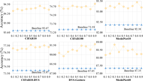
Figure 2: Influence of the balance coefficient $\alpha$ on the performance. As a whole, our method is insensitive to $\alpha$ and consistently outperforms the baseline.

Experiments

To confirm the effectiveness and generalizability of our method, we conduct experiments on the tasks of static object recognition (CIFAR10/100 and ImageNet-1K (Deng et al. 2009)), neuromorphic object/action recognition (CIFAR10-DVS (Li et al. 2017) and DVS-Gesture (Amir et al. 2017)), and 3D point cloud classification (ModelNet10/40 (Wu et al. 2015)) using VGG-9 (Ding et al. 2024), MS-ResNet18 (Hu et al. 2024), Spike-driven Transformer (Yao et al. 2023), PointNet (Qi et al. 2017a), and PointNet++ (Qi et al. 2017b) architectures. If not specified, the SNN timestep was 5 for neuromorphic datasets and 2 for static datasets. The experimental details can be found in Appendix B.

Ablation Studies

Method	TR	FH	CIFAR10	CIFAR100	CIFAR10-DVS	DVS-Gesture	ModelNet10	ModelNet40
Baseline			93.67	73.39	73.97	87.85	92.38	87.35
+TR	✓		$94.18_{+0.51}$	$74.45_{+1.06}$	$76.87_{+2.90}$	$91.32_{+3.47}$	$93.20_{+0.82}$	$87.86_{+0.41}$
+FH		✓	$94.02_{+0.35}$	$73.81_{+0.42}$	$75.33_{+1.36}$	$90.16_{+2.31}$	$93.26_{+0.88}$	$88.16_{+0.81}$
TRT	✓	✓	$\textbf{94.45}_{+0.78}$	$\textbf{74.85}_{+1.46}$	$\textbf{77.60}_{+3.63}$	$\textbf{91.67}_{+3.82}$	$\textbf{93.45}_{+1.07}$	$\textbf{88.84}_{+1.49}$

Table 1: Ablation study results (%) of the proposed method (TR: Temporal Reversal, FH: Feature Hybridization).

Method	Type	Architecture	T	CIFAR10	CIFAR100
RMP-Loss (Guo et al. 2023)${}^{ICCV}$	Surrogate gradient	VGG-16	10	94.39	73.30
CLIF (Huang et al. 2024)${}^{ICML}$	Surrogate gradient	ResNet-18	4	94.89	77.00
SSCL (Zhang et al. 2024)${}^{AAAI}$	Surrogate gradient	ResNet-20	2	93.40	69.81
NDOT (Jiang et al. 2024a)${}^{ICML}$	Forward-in-time	VGG-11	2	94.44	75.27
MS-ResNet (Hu et al. 2024)${}^{TNNLS}$	Surrogate gradient	MS-ResNet18	2	94.69*	73.84*
TAB (Jiang et al. 2024b)${}^{ICLR}$	Surrogate gradient	ResNet-19	2	94.73	76.31
SLT-TET (Anumasa et al. 2024)${}^{AAAI}$	Surrogate gradient	ResNet-19	2	94.96	73.77
Offset Spike (Hao et al. 2023)${}^{ICLR}$	Conversion	VGG-16	2	95.36	76.03
Spikformer (Zhou et al. 2023)${}^{ICLR}$	Surrogate gradient	Spiking Transformer-4-256	4	93.94	75.96
SDT (Yao et al. 2023)${}^{NeurIPS}$	Surrogate gradient	Spiking Transformer-2-512	2	94.91*	77.63*
TRT (Ours)	Surrogate gradient	VGG-9	2	94.45	74.85
		MS-ResNet18	2	95.13	76.14
		Spiking Transformer-2-512	2	95.61	79.43

Table 2: Comparative results (%) on static datasets. * denotes self-implementation results with open-source code.

Method	Type	Architecture	Spike-driven	Param (M)	T	ACC
MS-ResNet (Hu et al. 2024)${}^{TNNLS}$	Surrogate gradient	MS-ResNet34	✓	21.80	6	69.42
RMP-Loss (Guo et al. 2023)${}^{ICCV}$	Surrogate gradient	ResNet-34	✓	21.79	4	65.17
SSCL (Zhang et al. 2024)${}^{AAAI}$	Surrogate gradient	ResNet-34	✓	21.79	4	66.78
GAC-SNN (Qiu et al. 2024)${}^{AAAI}$	Surrogate gradient	MS-ResNet34	✓	21.93	4	69.77
Spikformer (Zhou et al. 2023)${}^{ICLR}$	Surrogate gradient	Spiking Transformer-8-768	✗	66.34	4	74.81
SDT (Yao et al. 2023)${}^{NeurIPS}$	Surrogate gradient	Spiking Transformer-8-768	✓	66.34	2	73.06$\diamond$ /74.32$\diamond{\dagger}$
					4	76.34$\diamond$ /77.07${\dagger}$
TRT (Ours)	Surrogate gradient	MS-ResNet34	✓	21.93	4	74.04
		Spiking Transformer-8-768	✓	66.34	2	74.01/74.77${\dagger}$

Table 3: Comparative results (%) on ImageNet. ${\dagger}$ denotes an inference resolution of $288\times 288$, the default resolution is $224\times 224$. $\diamond$ indicates a 2 timestep inference using a publicly available 4 timestep trained checkpoint.

Method	Type	Architecture	T	CIFAR10-DVS	DVS-Gesture
RMP-Loss (Guo et al. 2023)${}^{ICCV}$	Surrogate gradient	ResNet-20	10	75.60	-
NDOT (Jiang et al. 2024a)${}^{ICML}$	Forward-in-time	VGG-11	10	77.50${\dagger}$	-
TAB (Jiang et al. 2024b)${}^{ICLR}$	Surrogate gradient	VGG-9	5	74.57*	90.86*
SLT (Anumasa et al. 2024)${}^{AAAI}$	Surrogate gradient	VGG-9	5	74.23*	89.35*
SSNN (Ding et al. 2024)${}^{AAAI}$	Surrogate gradient	VGG-9	5	73.63	90.74
SDT (Yao et al. 2023)${}^{NeurIPS}$	Surrogate gradient	Spiking Transformer-2-256	5	72.53*${\dagger}$	94.79*
TRT (Ours)	Surrogate gradient	VGG-9	5	77.60	91.67
		MS-ResNet18	5	74.60	92.82
		Spiking Transformerr-2-256	5	75.55${\dagger}$	96.88

Table 4: Comparative results (%) on neuromorphic datasets. * self-implementation results. ${\dagger}$ using data augmentation.

Method	Type	Architecture	T	ModelNet10	ModelNet40
PointNet (Qi et al. 2017a)${}^{CVPR}$	ANN	PointNet	-	93.31*	89.46*
PointNet++ (Qi et al. 2017b)${}^{NeurIPS}$	ANN	PointNet++	-	95.50*	92.16*
Converted SNN (Lan et al. 2023)${}^{ICCV}$	SNN	PointNet	16	92.75	88.17
Spiking PointNet (Ren et al. 2023)${}^{NeurIPS}$	SNN	PointNet	2	92.98*	87.58*
P2SResLNet (Wu et al. 2024)${}^{AAAI}$	SNN	P2SResLNet	1	-	89.20
TRT (Ours)	SNN	PointNet	2	93.45	88.84
		PointNet++	2	93.97	90.57
			1	93.31$\diamond$	89.65$\diamond$

Table 5: Comparative results (%) on point cloud classification. * self-implementation. $\diamond$ training: $T=2$, inference: $T=1$.

Hyperparameter Sensitivity Analysis

In Fig. 2, we have experimentally studied the influence of the balance coefficient $\alpha$ on the performance. The influence of $\alpha$ is most significant for the DVS-Gesture, where larger values of $\alpha$ yield obviously better results, due to the stronger regularization of the perturbations at this point, which effectively mitigates the overfitting of the model. Overall, $\alpha$ leads to only slight fluctuations in the performance of the SNN, while consistently outperforming the baseline, indicating that our method is not sensitive to $\alpha$. We set the value of $\alpha$ in later experiments based on the performance peaks in Fig. 2.

Comparison to Baseline

The ablation studies for our method are shown in Tab. 1, where the PointNet was used for ModelNet10/40 and VGG-9 for the other datasets, and ablation studies with other architectures (MS-ResNet and Spike-driven Transformer) can be found in Appendix C. Experimental results show that using our proposed temporal reversal (TR) and feature hybridization (FH) alone improves the performance of the baseline SNN, and the maximum performance gain is achieved when training with both together (TRT). It is worth noting that while our method yields performance gains on different tasks and architectures, TRT is more effective on the temporal datasets CIFAR10-DVS and DVS-Gesture compared to the static datasets, suggesting that TRT can be more productive on the temporal task.

Comparison with Existing Methods

Static Object Recognition

The comparative results on CIFAR10/100 are shown in Tab. 2. Our Transformer architecture TRT achieved 95.61% and 79.43% accuracy, respectively, surpassing these comparative methods. Even with VGG-9, TRT achieved 94.45% and 74.85% accuracy, still outperforming most methods. On ImageNet, our Spiking Transformer achieves an accuracy of 74.77% with $T=2$, outperforming other methods with the same timestep and even approaching the four timestep Spikformer (Zhou et al. 2023), as shown in the Tab. 3. Using the MS-ResNet34 architecture, our TRT again outperforms other ResNet SNNs, demonstrating the performance advantages of our method.

Neuromorphic Object/Action Recognition

As shown in Tab. 4, on CIFAR10-DVS and DVS-Gesture, our TRT achieves 77.60% and 96.88% accuracy, respectively, at $T=~{}5$, surpassing even the performance of RMP-Loss (Guo et al. 2023) and NDOT (Jiang et al. 2024a) with $T=10$. Compared to the comparative methods, our TRT achieves the optimal performance-latency balance.

3D Point Cloud Classification

Table 5 shows the comparative results on the point cloud classification task, where again our method achieves optimal SNN performance. P2SResLNet achieves 89.20% accuracy on ModelNet40 with computationally expensive 3D spiking residual blocks, while we outperform it by 0.45% at the same timestep using the lightweight PointNet++ architecture.

Influence of Feature Reversal Location

For static data, TRT temporally reverses the encoded spikes. We explored the influence of temporal reversal at different locations using VGG-9 on CIFAR10/100 (defaulted to stage 1), and the results are shown in Tab. 6. The later the location of the feature temporal reversal, the smaller the performance gain of the TRT, but it still outperforms the baseline model. This can be interpreted as when the reversal location is close to the rear of the SNN, very few subsequent layers are available to extract the reversed features, and thus the full efficacy of the perturbation is not exploited.

Reversal location	Stage 1	Stage 2	Stage 3	Baseline
CIFAR10	94.45	94.34	94.06	93.67
CIFAR100	74.85	74.67	74.40	73.39

Table 6: Influence of feature temporal reversal location (%). The further ahead of the location, the greater the performance gain, and it consistently outperforms the baseline.

Average Spiking Firing Rate Visualization

We have visualized the average spike firing rate (ASFR) of the first two stages in VGG-9 on CIFAR10-DVS in Fig. 3. Compared to the baseline, our method not only achieves better performance but also has a lower ASFR (ASFR is positively correlated with the energy overhead during deployment), indicating that our method is more suitable for training low-energy SNNs to be deployed on edge devices. For additional visualizations please refer to Appendix D.

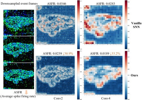
Figure 3: Visualization of ASFR. Our method has a lower ASFR than the baseline, favoring low-power deployment.

Conclusion

In this paper, we propose the TRT method to train SNNs with generalized spatio-temporal representations. TRT improves inference performance and reduces the spike firing rate by using simple temporal reversal and element-wise multiplication operations during training only. We demonstrate the effectiveness and versatility of TRT in static/neuromorphic object/action recognition and 3D point cloud classification tasks, achieving performance that exceeds existing methods. We expect our work to extend to more spatio-temporal scenarios and to facilitate research on high-performance, low-latency, low-power SNNs.

Appendix A Appendix A PyTorch-style Pseudocode Implementation

The PyTorch-style pseudocode for temporal reversal and spike firing rate hybridization is presented in Algorithm 2 and Algorithm 3 to facilitate the understanding and reproduction of our TRT method.

Algorithm 2 PyTorch-style code for temporal reversal

⬇

1# x: input data or encoded spikes.

2# x.shape: [T,B,C,H,W]

3# reversed_x: temporally reversed data or spikes.

4# reversed_x.shape: [T,B,C,H,W]

5def temporal_reversal(x):

6 T,B,C,H,W = x.shape

7 reversed_x = torch.zeros(x.shape)

8 for t in range(T):

9 reversed_x[t] = x[T+1-t]

10 return reversed_x

Algorithm 3 PyTorch-style code for spike firing rate hybridization

⬇

1

2# feat: spike feature.

3# reversed_feat: temporally reversed spike feature.

4# feat.shape=reversed_feat.shape: [T,B,C,H,W].

5# hybridized_fr: hybridized spike firing rate.

6# hybridized_fr.shape: [B,C,H,W]

7def firing_rate_hybridization(feat, reversed_feat):

8 T,B,C,H,W = feat.shape

9 fr = torch.zeros((B,C,H,W))

10 reversed_fr = torch.zeros(fr.shape)

11 for t in range(T):

12 fr += feat[t]

13 reversed_fr += reversed_feat[t]

14 fr /= T

15 reversed_fr /= T

16 hybridized_fr = fr * reversed_fr

17 return hybridized_fr

Appendix B Appendix B Experimental Details

Stage	VGG-9	MS-ResNet18	MS-ResNet34
0	-	Conv($3\times 3@64$)	Conv($7\times 7@64$)
$\left($			${\begin{array}[c]{@{}c@{}}$\left( \begin{array}[]{cc}\noindent\hbox{}\hfill{{\hbox{\begin{tabular}[c]{@{}c@{}}\text{Conv}(3 \times 3@64)\\ \text{Conv}(3 \times 3@64)\end{tabular}}\hbox{}\hfill}}\end{array} \right)\times 2 $\end{array}$}$
	averagepool(stride=2)	-	-
2	${\begin{array}[c]{@{}c@{}}Conv($3 \times 3$@256)\\ Conv($3 \times 3$@256)\end{array}$}$	( Conv(3 ×3@256) Conv(3 ×3@256) )×3	${\begin{array}[c]{@{}c@{}}$\left( \begin{array}[]{cc}\noindent\hbox{}\hfill{{\hbox{\begin{tabular}[c]{@{}c@{}}\text{Conv}(3 \times 3@128)\\ \text{Conv}(3 \times 3@128)\end{tabular}}\hbox{}\hfill}}\end{array} \right)\times 4 $\end{array}$}$
	averagepool(stride=2)	-	-
3	${\begin{array}[c]{@{}c@{}}Conv($3 \times 3$@512)\\ Conv($3 \times 3$@512)\end{array}$}$	( Conv(3 ×3@512) Conv(3 ×3@512) )×2	${\begin{array}[c]{@{}c@{}}$\left( \begin{array}[]{cc}\noindent\hbox{}\hfill{{\hbox{\begin{tabular}[c]{@{}c@{}}\text{Conv}(3 \times 3@256)\\ \text{Conv}(3 \times 3@256)\end{tabular}}\hbox{}\hfill}}\end{array} \right)\times 6 $\end{array}$}$
	avera

References

- Amir et al. (2017) Amir, A.; et al. 2017. A Low Power, Fully Event-Based Gesture Recognition System. In 2017 IEEE Conference on Computer Vision and Pattern Recognition (CVPR), 7388–7397.
- Anumasa et al. (2024) Anumasa, S.; Mukhoty, B.; Bojkovic, V.; De Masi, G.; Xiong, H.; and Gu, B. 2024. Enhancing Training of Spiking Neural Network with Stochastic Latency. In Proceedings of the AAAI Conference on Artificial Intelligence, volume 38, 10900–10908.
- Bal and Sengupta (2024) Bal, M.; and Sengupta, A. 2024. Spikingbert: Distilling bert to train spiking language models using implicit differentiation. In Proceedings of the AAAI conference on artificial intelligence, volume 38, 10998–11006.
- Chakraborty et al. (2024) Chakraborty, B.; Kang, B.; Kumar, H.; and Mukhopadhyay, S. 2024. Sparse Spiking Neural Network: Exploiting Heterogeneity in Timescales for Pruning Recurrent SNN. In The Twelfth International Conference on Learning Representations.
- Chen and He (2021) Chen, X.; and He, K. 2021. Exploring Simple Siamese Representation Learning. In Proceedings of the IEEE/CVF Conference on Computer Vision and Pattern Recognition (CVPR), 15750–15758.
- Cubuk et al. (2018) Cubuk, E. D.; Zoph, B.; Mane, D.; Vasudevan, V.; and Le, Q. V. 2018. AutoAugment: Learning Augmentation Policies from Data. arXiv:1805.09501.
- Deng et al. (2009) Deng, J.; Dong, W.; Socher, R.; Li, L.-J.; Li, K.; and Fei-Fei, L. 2009. Imagenet: A large-scale hierarchical image database. In 2009 IEEE conference on computer vision and pattern recognition, 248–255. Ieee.
- Ding et al. (2024) Ding, Y.; Zuo, L.; Jing, M.; He, P.; and Xiao, Y. 2024. Shrinking Your TimeStep: Towards Low-Latency Neuromorphic Object Recognition with Spiking Neural Networks. In Proceedings of the AAAI Conference on Artificial Intelligence, 11811–11819.
- Ding et al. (2023) Ding, Y.; Zuo, L.; Yang, K.; Chen, Z.; Hu, J.; and Xiahou, T. 2023. An improved probabilistic spiking neural network with enhanced discriminative ability. Knowledge-Based Systems, 280: 111024.
- Duan et al. (2022) Duan, C.; Ding, J.; Chen, S.; Yu, Z.; and Huang, T. 2022. Temporal Effective Batch Normalization in Spiking Neural Networks. In Koyejo, S.; Mohamed, S.; Agarwal, A.; Belgrave, D.; Cho, K.; and Oh, A., eds., Advances in Neural Information Processing Systems, volume 35, 34377–34390. Curran Associates, Inc.
- Fang et al. (2023) Fang, W.; Chen, Y.; Ding, J.; Yu, Z.; Masquelier, T.; Chen, D.; Huang, L.; Zhou, H.; Li, G.; and Tian, Y. 2023. SpikingJelly: An open-source machine learning infrastructure platform for spike-based intelligence. Science Advances, 9(40): eadi1480.
- Guo et al. (2024) Guo, Y.; Chen, Y.; Liu, X.; Peng, W.; Zhang, Y.; Huang, X.; and Ma, Z. 2024. Ternary spike: Learning ternary spikes for spiking neural networks. In Proceedings of the AAAI Conference on Artificial Intelligence, volume 38, 12244–12252.
- Guo et al. (2023) Guo, Y.; Liu, X.; Chen, Y.; Zhang, L.; Peng, W.; Zhang, Y.; Huang, X.; and Ma, Z. 2023. RMP-Loss: Regularizing Membrane Potential Distribution for Spiking Neural Networks. In Proceedings of the IEEE/CVF International Conference on Computer Vision (ICCV), 17391–17401.
- Hao et al. (2023) Hao, Z.; Ding, J.; Bu, T.; Huang, T.; and Yu, Z. 2023. Bridging the Gap between ANNs and SNNs by Calibrating Offset Spikes. In The Eleventh International Conference on Learning Representations.
- Hinton, Vinyals, and Dean (2015) Hinton, G.; Vinyals, O.; and Dean, J. 2015. Distilling the Knowledge in a Neural Network. arXiv:1503.02531.
- Hu et al. (2024) Hu, Y.; Deng, L.; Wu, Y.; Yao, M.; and Li, G. 2024. Advancing Spiking Neural Networks Toward Deep Residual Learning. IEEE Transactions on Neural Networks and Learning Systems, 1–15.
- Huang et al. (2024) Huang, Y.; LIN, X.; Ren, H.; FU, H.; Zhou, Y.; LIU, Z.; biao pan; and Cheng, B. 2024. CLIF: Complementary Leaky Integrate-and-Fire Neuron for Spiking Neural Networks. In Forty-first International Conference on Machine Learning.
- Jiang et al. (2024a) Jiang, H.; Masi, G. D.; Xiong, H.; and Gu, B. 2024a. NDOT: Neuronal Dynamics-based Online Training for Spiking Neural Networks. In Forty-first International Conference on Machine Learning.
- Jiang et al. (2024b) Jiang, H.; Zoonekynd, V.; Masi, G. D.; Gu, B.; and Xiong, H. 2024b. TAB: Temporal Accumulated Batch Normalization in Spiking Neural Networks. In The Twelfth International Conference on Learning Representations.
- Kamata, Mukuta, and Harada (2022) Kamata, H.; Mukuta, Y.; and Harada, T. 2022. Fully spiking variational autoencoder. In Proceedings of the AAAI Conference on Artificial Intelligence, volume 36, 7059–7067.
- Kim et al. (2023) Kim, Y.; Li, Y.; Park, H.; Venkatesha, Y.; Hambitzer, A.; and Panda, P. 2023. Exploring temporal information dynamics in spiking neural networks. In Proceedings of the AAAI Conference on Artificial Intelligence, volume 37, 8308–8316.
- Krizhevsky, Hinton et al. (2009) Krizhevsky, A.; Hinton, G.; et al. 2009. Learning multiple layers of features from tiny images.
- Lan et al. (2023) Lan, Y.; Zhang, Y.; Ma, X.; Qu, Y.; and Fu, Y. 2023. Efficient Converted Spiking Neural Network for 3D and 2D Classification. In Proceedings of the IEEE/CVF International Conference on Computer Vision (ICCV), 9211–9220.
- Li et al. (2024) Li, B.; Leng, L.; Shen, S.; Zhang, K.; Zhang, J.; Liao, J.; and Cheng, R. 2024. Efficient Deep Spiking Multilayer Perceptrons With Multiplication-Free Inference. IEEE Transactions on Neural Networks and Learning Systems, 1–13.
- Li et al. (2017) Li, H.; Liu, H.; Ji, X.; Li, G.; and Shi, L. 2017. CIFAR10-DVS: An Event-Stream Dataset for Object Classification. Frontiers in Neuroscience, 11.
- Ma et al. (2024) Ma, X.; Dai, X.; Bai, Y.; Wang, Y.; and Fu, Y. 2024. Rewrite the Stars. In Proceedings of the IEEE/CVF Conference on Computer Vision and Pattern Recognition (CVPR), 5694–5703.
- Ponghiran and Roy (2022) Ponghiran, W.; and Roy, K. 2022. Spiking neural networks with improved inherent recurrence dynamics for sequential learning. In Proceedings of the AAAI Conference on Artificial Intelligence, volume 36, 8001–8008.
- Qi et al. (2017a) Qi, C. R.; Su, H.; Mo, K.; and Guibas, L. J. 2017a. PointNet: Deep Learning on Point Sets for 3D Classification and Segmentation. In Proceedings of the IEEE Conference on Computer Vision and Pattern Recognition (CVPR).
- Qi et al. (2017b) Qi, C. R.; Yi, L.; Su, H.; and Guibas, L. J. 2017b. PointNet++: Deep Hierarchical Feature Learning on Point Sets in a Metric Space. In Guyon, I.; Luxburg, U. V.; Bengio, S.; Wallach, H.; Fergus, R.; Vishwanathan, S.; and Garnett, R., eds., Advances in Neural Information Processing Systems, volume 30. Curran Associates, Inc.
- Qiu et al. (2024) Qiu, X.; Zhu, R.-J.; Chou, Y.; Wang, Z.; Deng, L.-j.; and Li, G. 2024. Gated attention coding for training high-performance and efficient spiking neural networks. In Proceedings of the AAAI Conference on Artificial Intelligence, volume 38, 601–610.
- Ren et al. (2023) Ren, D.; Ma, Z.; Chen, Y.; Peng, W.; Liu, X.; Zhang, Y.; and Guo, Y. 2023. Spiking PointNet: Spiking Neural Networks for Point Clouds. In Oh, A.; Naumann, T.; Globerson, A.; Saenko, K.; Hardt, M.; and Levine, S., eds., Advances in Neural Information Processing Systems, volume 36, 41797–41808. Curran Associates, Inc.
- Shawe-Taylor and Cristianini (2004) Shawe-Taylor, J.; and Cristianini, N. 2004. Kernel methods for pattern analysis. Cambridge university press.
- Srivastava et al. (2014) Srivastava, N.; Hinton, G.; Krizhevsky, A.; Sutskever, I.; and Salakhutdinov, R. 2014. Dropout: a simple way to prevent neural networks from overfitting. The journal of machine learning research, 15(1): 1929–1958.
- Su et al. (2023) Su, Q.; Chou, Y.; Hu, Y.; Li, J.; Mei, S.; Zhang, Z.; and Li, G. 2023. Deep Directly-Trained Spiking Neural Networks for Object Detection. In Proceedings of the IEEE/CVF International Conference on Computer Vision (ICCV), 6555–6565.
- Wang and Yu (2024) Wang, L.; and Yu, Z. 2024. Autaptic Synaptic Circuit Enhances Spatio-temporal Predictive Learning of Spiking Neural Networks. In Forty-first International Conference on Machine Learning.
- Wang et al. (2022) Wang, X.; Fan, H.; Tian, Y.; Kihara, D.; and Chen, X. 2022. On the Importance of Asymmetry for Siamese Representation Learning. In Proceedings of the IEEE/CVF Conference on Computer Vision and Pattern Recognition (CVPR), 16570–16579.
- Wu et al. (2022) Wu, J.; Xu, C.; Han, X.; Zhou, D.; Zhang, M.; Li, H.; and Tan, K. C. 2022. Progressive Tandem Learning for Pattern Recognition With Deep Spiking Neural Networks. IEEE Transactions on Pattern Analysis and Machine Intelligence, 44(11): 7824–7840.
- Wu et al. (2024) Wu, Q.; Zhang, Q.; Tan, C.; Zhou, Y.; and Sun, C. 2024. Point-to-Spike Residual Learning for Energy-Efficient 3D Point Cloud Classification. In Proceedings of the AAAI Conference on Artificial Intelligence, volume 38, 6092–6099.
- Wu et al. (2018) Wu, Y.; Deng, L.; Li, G.; Zhu, J.; and Shi, L. 2018. Spatio-Temporal Backpropagation for Training High-Performance Spiking Neural Networks. Frontiers in Neuroscience, 12.
- Wu et al. (2015) Wu, Z.; Song, S.; Khosla, A.; Yu, F.; Zhang, L.; Tang, X.; and Xiao, J. 2015. 3D ShapeNets: A Deep Representation for Volumetric Shapes. In Proceedings of the IEEE Conference on Computer Vision and Pattern Recognition (CVPR).
- Yao et al. (2023) Yao, M.; Hu, J.; Zhou, Z.; Yuan, L.; Tian, Y.; Xu, B.; and Li, G. 2023. Spike-driven Transformer. In Oh, A.; Naumann, T.; Globerson, A.; Saenko, K.; Hardt, M.; and Levine, S., eds., Advances in Neural Information Processing Systems, volume 36, 64043–64058. Curran Associates, Inc.
- Yuan et al. (2020) Yuan, L.; Tay, F. E.; Li, G.; Wang, T.; and Feng, J. 2020. Revisiting Knowledge Distillation via Label Smoothing Regularization. In Proceedings of the IEEE/CVF Conference on Computer Vision and Pattern Recognition (CVPR).
- Zhang et al. (2019) Zhang, L.; Song, J.; Gao, A.; Chen, J.; Bao, C.; and Ma, K. 2019. Be Your Own Teacher: Improve the Performance of Convolutional Neural Networks via Self Distillation. In 2019 IEEE/CVF International Conference on Computer Vision (ICCV), 3712–3721.
- Zhang et al. (2024) Zhang, Y.; Liu, X.; Chen, Y.; Peng, W.; Guo, Y.; Huang, X.; and Ma, Z. 2024. Enhancing Representation of Spiking Neural Networks via Similarity-Sensitive Contrastive Learning. In Proceedings of the AAAI Conference on Artificial Intelligence, volume 38, 16926–16934.
- Zhou et al. (2023) Zhou, Z.; et al. 2023. Spikformer: When Spiking Neural Network Meets Transformer. In The Eleventh International Conference on Learning Representations.
- Zuo et al. (2024) Zuo, L.; Ding, Y.; Jing, M.; Yang, K.; and Yu, Y. 2024. Self-Distillation Learning Based on Temporal-Spatial Consistency for Spiking Neural Networks. arXiv:2406.07862.