Key Motifs Searching in Complex Dynamical Systems
Abstract
Key network motifs searching in complex networks is one of the crucial aspects of network analysis. There has been a series of insightful findings and valuable applications for various scenarios through the analysis of network structures. However, in dynamic systems, slight changes in the choice of dynamic equations and parameters can alter the significance of motifs. The known methods are insufficient to address this issue effectively. In this paper, we introduce a concept of perturbation energy based on the system’s Jacobian matrix, and define motif centrality for dynamic systems by seamlessly integrating network topology with dynamic equations. Through simulations, we observe that the key motifs obtained by the proposed energy method present better effective and accurate than them by integrating network topology methods, without significantly increasing algorithm complexity. The finding of key motifs can be used to apply for system control, such as formulating containment policies for the spread of epidemics and protecting fragile ecosystems. Additionally, it makes substantial contribution to a deeper understanding of concepts in physics, such as signal propagation and system’s stability.
keywords:
Key motifs , Complex networks , Dynamical systems , Collective behavior , Epidemic process.PACS:
89.75.-k , 05.45.-a , 89.75.Fb , 05.45.Gg , 05.10.-a.[first]organization=School of Mathematical Sciences, Shanghai Jiao Tong University,city=Shanghai, postcode=200240, state=Shanghai, country=China \affiliation[second]organization=Ministry of Education (MOE) Funded Key Lab of Scientific and Engineering Computing, Shanghai Jiao Tong University,city=Shanghai, postcode=200240, state=Shanghai, country=China \affiliation[third]organization=Shanghai Center for Applied Mathematics (SJTU Center), Shanghai Jiao Tong University,city=Shanghai, postcode=200240, state=Shanghai, country=China
![[Uncaptioned image]](/html/2408.08932/assets/x1.png)
A new concept for perturbation energy is proposed, which is applicable to all types of perturbations.
Based on dynamical system and network structure, a new motif centrality and motif ranking algorithm is proposed, which performs better effective and accurate than some known algorithms based on network topology.
The proposed ranking algorithm can be applied for the control of spreading diseases, and offer a more flexible, scientific, and minimally disruptive containment policy compared to common lockdown policies.
The proposed ranking algorithm can be applied to the protection of ecosystems and the control of gene regulation, offering a more effective method to achieve specific goals.
1 Introduction
Dynamical systems serve as powerful tools for monitoring the evolution of real world systems over time, and extensive researches on dynamical systems has significantly enhanced our understanding of various physical phenomenon. For instance, the study of signal propagation contributes to our insights of dynamic processes like the spread of infectious diseases or violence[1, 2, 3, 4, 5, 6, 7], while investigations into network stability and resilience deepen our awareness of ecological system tipping points[8, 9, 10, 11, 12]. By leveraging specific dynamics properties, we can manipulate either the network structure or certain parameters within the network dynamics to achieve a specific objectives, referred to as network control[13, 14, 15, 16, 17, 18], such as restoring system stability or reaching a particular fixed state. In this paper, we concentrate on control of the network structure and explore how motifs affect the properties of dynamical systems.
Network motifs, which can be categorized into undirected motifs and directed motifs, are fundamental building blocks of complex networks[19]. Some common motifs, such as edges[20, 21], nodes[22, 23], and cycles[24, 25, 26, 27], all of which can significantly impact network properties and dynamics properties[28, 29, 30, 31]. A comprehensive exploration of network motifs is essential for understanding dynamics, particularly in identifying motifs with significant impacts on dynamic properties. This offers a new approach to comprehend network structure and dynamic behavior. Furthermore, such research holds significant importance in various fields, including dynamic system control[32], infectious disease prevention and control[26], information dissemination[4, 5].
From now on, numerous significant conclusions have been drawn regarding the centrality of network motifs. Among these, node centrality is the most extensively studied, encompassing aspects such as local topological properties, global topological properties, spectral properties, and propagation properties[22]. Various node centrality measures are employed depending on different cases and objectives to achieve specific goals. In recent studies, more interesting concepts and algorithms have emerged. For example, Changjun Fan et al. introduced reinforcement learning to identify key players in complex network[33]. Additionally, Siyang Jiang et al. used the Fiedler vector to rank cycles in network[27], which is somewhat related to community detection. All of these findings have significant implications for controlling network dynamics.
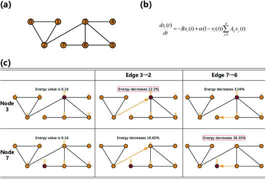
However, in dynamical systems, key nodes or edges are dynamically changing, as they are are influenced by the state of nodes and the interaction connections evolving them. To illustrate this point, we consider a toy model and epidemic dynamics, and present the results in Figure 1. In this simulation, we utilize the norm of the node state vector to represent the overall energy of the dynamical system, and apply fixed perturbations to different nodes, serving as perturbed nodes. It can be observed that the final state of the nodes varies depending on the selected perturbed node. Moreover, when restricting the same edge in two dynamical systems, we reach completely opposite conclusions: for the case with perturbed node , constraining the edge leads to a greater decrease in state compared to constraining . Conversely, in the case with perturbed node , the situation is reversed, and the impact of edge varies significantly with different source node choices.(Note that represents is the source node and is the target node, and we can set value for (or (j,i)) to control this arrow.) This underscores the inadequacy of solely considering edge centrality based on network structure without incorporating dynamic behavior, and emphasizes the necessity to devise the motifs centrality that comprehensively consider both dynamic equations and network topology.
In this paper, we introduce a centrality for identifying key motifs based on the inverse of the Jacobian matrix, which takes into account both network topology and dynamics and can determine the importance of motifs at a specific state. Unlike fixed network centrality, our proposed centrality may vary depending on different dynamical models or selections of dynamical parameters. This allows us to dynamically and accurately characterize the system’s properties. Furthermore, the Jacobian matrix is a fundamental concept in dynamical systems and plays a crucial role in the studying network stability and signal propagation. It captures the linear variation properties that the node states satisfy at a given time. Our in-depth examination of the Jacobian matrix enhances our understanding of this mathematical concept, enabling us to further investigate the physical mechanisms of propagation and apply them to other physical domains.
2 Framework on Motifs Searching for Dynamical Systems
2.1 Energy of Perturbation
In this paper, we consider a dynamical system with nodes:
| (1) |
in which represents a set of nonlinear functions, and denotes a general interaction matrix, encompassing both binary matrices and weighted matrices. For simplicity, we can divide this system into self-dynamics and dynamical interaction, expressed as [8]. Moreover, the interaction between node and its neighborhood nodes can be simplified as [3]. The general dynamical model proposed in Eq.(1) can unveil various dynamics model based on different choices of nonlinear functions, such as epidemic dynamics, biochemical dynamics, etc.
The stationary state in the unperturbed dynamical system, denoted as , is obtained by setting the left hand of Eq.(1) to be , i.e. . The signal propagation process is defined by introducing a perturbation to the stationary state of a node , and the shifted state of node is characterized by . Furthermore, we can separate its initial state and dynamics equation by letting and . (It’s important to note that the perturbation in this article is not independent from time , and the signal propagation proposed in the previous research[3, 4, 5] can be achieved by setting ). This perturbation can drive nodes in this systems to their own shifted states . Furthermore, the perturbation for shifted states satisfies the following dynamic equation, as obtained from [4, 5, 11]:
| (2) |
in which represents the controlling vector for node , where denotes the th column of the identity matrix. is the perturbed Jacobian matrix, obtained by replacing the entries in the -th rows of with zero[5]. The Jacobian matrix is defined as , and the perturbed Jacobian matrix can be expressed as .
According to the Laplace transformation method outlined in Hu et al.’s work[5], the solution for Eq.(1) can be expressed using a matrix exponential function . will converge to a non-zero constant vector [5], referred to as the shifted state of node . This constant can be obtained using the limiting theorem of the Laplace transform for Eq.(2), and there is
| (3) |
where is the corresponding variable to time and . Utilizing the Sherman-Morrison formula and considering the fact , Eq.(3) can be simplified as
| (4) |
in which, according to the dynamical equation for , we have , and represents the value of matrix on the -th row and -col, equivalent to (the detailed proof has been provided in the Appendix A.1). Then, We then define the energy of perturbation on node as the norm of (introduced in Eq.(4)), i.e.
| (5) |
Through the definition of energy, if we assume the Jocabian matrix is symmetric, then can be expressed as . This specific case is analogous to expectation value and variance of random variables. The discrepancy between numerator and denominator is introduced by values in the -th row and the -th col of .
2.2 Centrality of Motifs
Through the definition of energy of perturbation proposed in Eq.(5), each edge in the network contributes to this value(Note that here an edge here is considered as a directed arrow). The energy for the entire network arises from interactions among the energies associated with each edge. Therefore, it’s not feasible to directly isolate the energy for only one edge from this intricate interaction. Here, we present an error analysis method, which involves introducing a small perturbation value to a set of edges . This perturbation affects the Jacobian matrix , where , resulting in a perturbed energy denoted as . For simplicity in calculation, we consider two matrices: and , corresponding to the numerator and the denominator of Eq.(5). Through some calculations, the change in energy between the original energy and the perturbed energy can be obtained as(the detailed proof has been provided in the Appendix A.2):
| (6) | ||||
where the relative difference can be calculated from Eq.(6), and
| (7) |
Next, we estimate the values of and using the error analysis method. Firstly, according to the definition of the inverse matrix, we have . Here, we assume and are matrices of order , so and are matrices of order . Then, we only consider order and obtain . Finally, by substituting the value of into , we can obtain the exact estimation for :
| (8) |
Similarly, according to the definition of inverse matrix, we have . Here, , , in this formula are matrices of order . Then, we ignore terms of order and higher, and obtain . Finally, by substituting the value of into , and we can obtain the exact estimation for :
| (9) |
In this paper, we provide a definition of centrality of motifs under the concept of energy of perturbation, and let . Substituting the value of from Eq.(9) and value of from Eq.(8) into Eq.(7), there should be
| (10) |
Therefore, we obtain the motif score , representing the centrality of motif .
Specifically for centrality of nodes, we can fix a node and select , then we can obtain
If , then , and the change in energy , this suggests that our energy of perturbation is also applicable for node centrality.
Through the estimation for proposed in Eq.(10), we can determine the importance of motifs solely based on the Jacobian matrix. This approximation encapsulates information about perturbations, which can provide better predictions for dynamical system compared to static centrality, such as node centrality or eigenvector vector. Using our motif centrality, we can estimate key nodes, edges, or cycles in a dynamical system, the detailed algorithm has been provided in Algorithm 1.
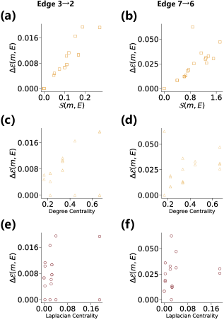
To highlight the advantages of our motif centrality, we compare two static centrality in complex network: the first is the degree centrality , which calculates the expectation number of edges between node and based on homogeneous assumption. Here, represents the degree of node . The second is the Laplacian centrality, introduced in Jiang et al.’s work[27], is defined as , where is the Filder vector of the network. We preform simulations on the network depicted in Figure 1, respectively perturbing on node and limiting edge , and similarly for node and edge , and investigate relationship between the motif centrality and the change in energy . The change in energy can represent the signal propagated through motifs, especially if we select , it can interpreted as the effect of deleting one motif. The results are shown in Figure 2, indicating that our motif centrality can better monitor the change in energy regardless of which node is perturbed, while the other two centrality do not have a clear correlation.
Furthermore, our motif centrality requires the values of the row and column of inferred in motifs set , with a computational complexity of . In comparison, the degree centrality is related to the number of edges in the network, with a complexity of , where is the average degree of the network. The Laplacian centrality is related to the eigenvector corresponding to the second smallest eigenvalue of the Laplacian matrix, with a complexity of . It is evident that our motif centrality does not have a significant disadvantage in algorithmic complexity and consistently outperforms the other two centrality in terms of results.
3 Applications to Epidemic Dynamics
Infectious diseases are illnesses caused by pathogens that can be transmitted among humans, animals, and between humans and animals. The spread of an infectious disease can have significant impacts on production, livelihoods, and the health of thousands of people. With the rapid development of society productive forces and transportation systems, the rate of spread for infectious diseases is expected to be more severe compared to ancient times. In the 21st century, China alone has witnessed several large-scale infectious disease outbreaks, such as the SARS epidemic in 2004[34, 35] and the COVID-19 epidemic in 2021[36, 37, 38]. To ensure the safety of the general population and maintain the normal functioning of the national economic, the governments and relevant departments must need to monitor and predict the spread of infectious diseases. This requires the assistance of mathematical tools to formulate effective policies for controlling.
In mathematics, epidemic dynamics are usually used to characterize the population changes in different groups during the spread of an infectious disease. Common epidemic dynamics include the , , , , where , , and respectively represents the proportion of the susceptible[39, 40], exposed, infected and recovered individuals. These groups interact each other based on certain physical laws, undergoing transitions with specific probabilities. For example, susceptible individuals () can become exposed () through a certain reproduction number , exposed individuals() go through a latent period () to become infected (), and infected individuals go through a recovery period () to become recovered ()[38, 41]. It’s important to note that the recovered individuals() include both those who have recovered or died, and they do not revert to being susceptible, reflecting the realities of infectious diseases where recovery leads to short-term immunity.
The model for these four groups can depict the process of the spread of an epidemic in human society and play a crucial role in multiple epidemic predictions and control efforts. It provides strong theoretical support and data feedback for formulating epidemic controlling policies, allocating rescue materials, managing medical resources, and deciding on lockdown policies. In this paper, we focus on the change in susceptible individuals (), with its general formula being[42]
| (11) |
in which is the ratio of susceptible individuals at time , is the recovery rate and denotes the infection rate, corresponding respectively to / and . The actual value of is influenced by the characteristics of disease. Infectious diseases transmitted through simple behaviors, such as airborne or respiratory transmission, often have a higher , as observed in cases like SARS and COVID-19. Conversely, diseases spread through complex behaviors like fluid or blood transmission tend to have a lower , as seen in diseases like HIV and syphilis.
3.1 Verification of Theoretical Framework
In the real world, the outbreak of infectious diseases often originates in one or a few cities and then spreads to other countries/area. It is widely accepted that outbreak typically start from a single city. To limit the spread, governments need to implement relevant policies, including lockdowns and restrictions on travel between cities. In field of complex networks, lockdowns can be considered as removing all connections of a specific node with other nodes in the network, while restricting travel between cities can be seen as removing one or several edges in the network. Surprisingly, these two policies align well with the concept of network centrality and motif searching proposed in this paper, and the essential policy should be promulgated based on the motifs with the highest centrality.
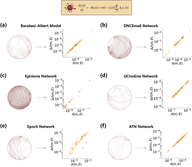
To validate and refine our theoretical framework, we utilize epidemic dynamics to simulate the spread of diseases on real networks and conduct applied analyses in real-world cases. In this section, we employ changes in the energy of perturbation to monitor the spread and compare this value with our centrality proposed in Eq.(10). Simulations are preformed on the Barabási-Albert model and five other real networks: the first is DNCEmail network (DNCEmail), a network of emails from the 2016 democratic national committee email leak, consisting of 1834 nodes and 4367 edges[43]. The second is Epinions network (Epinions), a binary online social network consisting of 467 nodes and 6538 edges[44]. The third is UCIonline network (UCIonline), a collects real-time information networks of UC-Irvine students over a 218-day period, consisting of 1893 nodes and 27670 edges[45]. The fourth is Email epoch network (Epoch), a scale-free network collected email social networks over a 6-month period, consisting of 3185 nodes and 31885 edges [46]. The fifth is Advogato trust network (ATN), a symmetric social network constructed from connections within the community of open source developers, consisting of 539 nodes and 23540 links [47]. We removed the edges in the suggested epidemic networks and simulated the observed change in energy . The simulation results, as depicted in Figure 3, clearly demonstrate that our theoretical predictions align perfectly with the observed change in energy in real-world cases, this validates the correctness of our theoretical framework and the effectiveness of our motif centrality.
3.2 Advice to Lockdown Policy
In this section, we will present evidence for the effectiveness of our theoretical framework in disease control. After an outbreak of infectious disease, governments are limited by a certain timeframe to gather information about the epidemic and then implement corresponding control policy. Issuing reasonable policies for disease spread involves finding a balance between ensuring public safety and allowing continuous economic activities. For example, complete relaxation without any control policies poses a significant threat to public healthy, while overly strict control policies can hinder economic activities, severely impacting people’s livelihoods and daily lives. Even a lockdown policy for a city can directly affects the lives of its residents and introduce instability factors into society. Hence, determining when and how to choose an appropriate level of control under scientific guidance and mathematical assistance become crucial. In this paper, we propose a framework for restricting interactions between two nodes/cities based on our proposed edge motif centrality, prioritizing pairs of nodes with the highest motif centrality. Compared to the rigid lockdown policies, our approach is more flexible, efficient, and ensures the normal functioning of daily life, which has significant practical value.
In our framework, we utilize the energy to gauge the severity of infectious disease spread, and mitigate it by selectively removing edges between network nodes. It is evident that the change in energy represents the importance of choice of edge set . However, removing more edges will have a greater impact on the original societal activities. This prompts us to balance the relationship between the size of edge set and , aiming to restrict disease spread while minimizing disruption to the
overall network connectivity. We define efficiency for edge set as the ratio , with the goal of identify the edge set with the highest efficiency. In mainstream views, if we could precisely identify the source, removing the connections of that node with the external network would be sufficient. However, due to the lag of information, deleting the connection to the perturbed node at this time may not be the most effective, as the disease has already spread throughout the network. This emphasizes the need for a robust guiding strategy. Through our motif ranking algorithm, as described in Algorithm 1, we can assign centrality values to all edges using Eq.(10), and obtain by selecting edges with the highest motif centrality . This algorithm allows us to select one edge at a time.
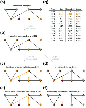
To illustrate this concept, we preform an epidemic simulation on the network proposed in Figure 1. After a certain period of continuous perturbation to a node in the network, we compare the final infection outcomes under different policies (Note that we examine the dynamic system after ”a certain period of perturbation” to consider the time required for the government to gather specific information about the infectious disease and determine the policy). We present our results in Figure 4 by perturbing node and restricting edges and . In comparison, we observe that the proportion of deleted directed edges in the entire network is only , but the overall network energy decreases by , and the network energy excluding the perturbed node decreases by . The efficiency excluding the perturbed node is by times higher than deleting all edges! While For the two directed edges identified by the Laplacian centrality or degree centrality rankings, such as and for Laplacian centrality, the final energy is much larger compared to the energy restricted by our centrality measure. This example indicates employing scientific control policies can enhance the reliability, rationality, and robustness of policy formulation, yielding better results compared to other centrality measures.
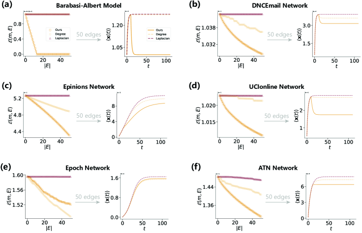
Furthermore, we conducted simulations on the theoretical network and five real networks mentioned in Figure 3. We calculate the perturbed energy of system over size of , and the average state of nodes after restricting certain edges over time . All of these result are compared with both the degree centrality and Laplacian centrality, and are presented in Figure 5. It is evident that our centrality can effectively decrease centrality of motif and can deeply affect average state of dynamical system. Moreover, our result consistently outperformed the other two centrality in almost all scenarios, and the significant reduction in control under a small number of restricted edges indicates that our centrality has a distinct advantage in addressing infectious disease prevention and control.
4 Applications to Mutualistic Dynamics
Research in ecosystems is a popular topic in complex networks. With the development of human society and the widespread acceptance of ecological values, maintaining the stability of ecosystems and protecting biodiversity have become issues of concern for governments and relevant departments. Empirically, it is believed that the more complex the system species, the more robust the system is. However, Robert May published a groundbreaking article[48], providing a theorem that the stability of a system decreases with the increase in network size and interaction strength. Detailed mathematical proofs reveal extremely different physical laws, indicating that the study of ecosystems requires the introduction of a large number of tools from complex networks.
In mathematical models, we generally consider the following three types of interactions between species in biology. The first type is predation: for example, the relationship between predator and prey , where has an inhibitory effect on (denoted by ), and has a mutualistic effect on (denoted by )[49]. The second type of relationship is intra-population competition: for example, the relationship between species and species due to competition for the same resources, where there is an inhibitory effect between and (denoted by )[49]. The third type of relationship is mutualism within populations: for example, the parasitic relationship between species and species , where there is a mutualistic effect between and (denoted by )[49]. The combination and interactions of these three types of relationships form the basic impact patterns of an ecosystem.
In this section, we consider the mutualistic relationships between species, which are related to building stable, robust ecosystems. For example, the restoration of desert ecosystems and the protection of river/sea ecosystems both require external interventions to ensure the maintenance of mutual promotion among species. The general expression for mutualistic dynamics is[48, 50]:
| (12) |
in which is the group size of specie at time , is the reproducing process coefficient, is the opposite effect coefficient representing the competition due to limited resources, and captures the interaction strength between two species. In artificially maintained networks, interactions between weaker species typically result in smaller values of , requiring strong powers to maintain the stability of the ecosystem.
4.1 Verification of Theoretical Framework
In real ecosystems, we generally select two main approaches: introducing species and enhancing interactions between species. In the context of our framework, increasing the number of species is equivalent to adding state of nodes to the system, while strengthening interactions between species is akin to increasing the weights of edges (weakening interactions is equivalent to reducing weights or deleting edges). Therefore, edges with higher scores represent species relationships that require particular attention.
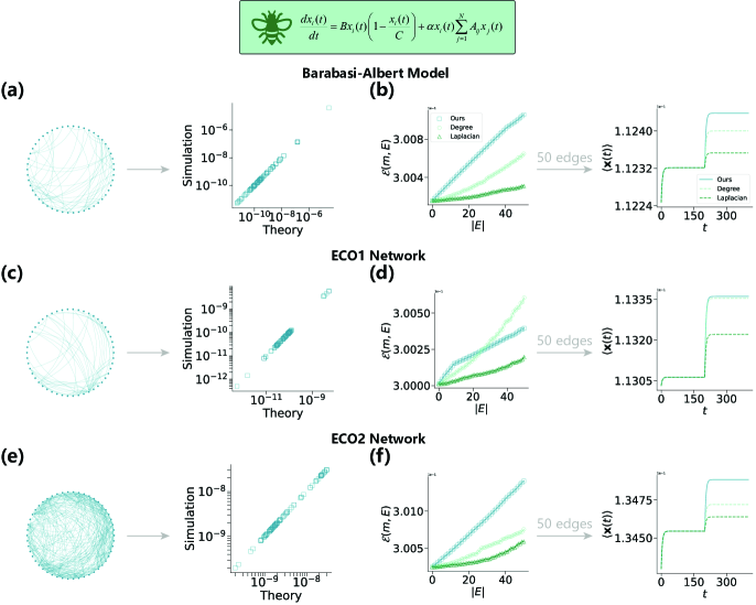
Simulations are preformed on the Barabási-Albert model and two real networks: in which these two networks are collected from the symbiotic interactions in Carlinville Illinois[51]. The interactions matrix between plants and pollinators is stored by a matrix with size , which can be expressed as a bipartite graph containing 456 plants and their 1429 pollinators. The first network is obtained from containing 456 nodes, and its academic name is the plant-plant mutualistic network(ECO1), there exists an edge between two plant and if density is larger than a threshold . The second is the pollinator-pollinator network(ECO2) containing 1429 nodes, edges are determined with density . Obviously, ECO1 and ECO2 are all symmetric networks. We included the weights of edges in the suggested ecosystem and simulated the observed change in energy . The simulation results have been illustrated in Figure 6 and clearly show that our theoretical results can perfectly predict in ecosystems and validates the correctness of our theoretical framework.
4.2 Advice to Ecological Protection
In some real-life ecosystems, simply increasing the number of organisms may not necessarily yield optimal results and can be cost-ineffective, as seen in the case of the failure of Biosphere 2. Therefore, it is necessary to enhance interactions between species during the process of species introduction to strengthen system stability. Methods to enhance interactions include constructing biological exchange pathways and protecting habitats. Efficient ecological conservation measures can protect fragile ecosystems to the maximum extent at minimal cost, safeguarding the living environment for human.
Then, we conducted simulations on the theoretical network and two real networks mentioned in Section 4.1. We calculated over the size of and after adding the weight of certain edges over time , where can signify the efficiency of increasing species diversity. These results were compared with both degree centrality and Laplacian centrality and are depicted in Figure 6. It is evident that in almost all cases our results consistently outperformed the other two centralities. The significant improvement in control under a small number of edges indicates that our centrality offers a distinct advantage in safeguarding fragile ecosystems.
5 Applications to Regulatory Dynamics
Gene regulation is a very important biochemical process, which is the mechanism that controls gene expression within an organism. It mainly involves the transcription of genes and the translation of mRNA. For multicellular organisms, gene regulation is closely related to cell differentiation and individual development. In mathematical models, we generally use the Michaelis-Menten dynamics to characterize the basic process of gene regulation. The basic expression is[52, 53, 54]:
| (13) |
in which the level of gene expression of gene at time . The different values of the parameter in the self-dynamics determine various biochemical processes. For instance, corresponds to the degradation process, while corresponds to the dimerization process. The interaction dynamics with is known as the Hill function, which records the cooperation level of gene by gene [53]. It possesses properties such as and , making it a switch-like dynamic. This function is similar to a gate function in neural networks. Due to the specific properties of the Hill function, only a subset of genes in gene interactions will actually have an effect[55].
5.1 Verification of Theoretical Framework
We still integrate the mechanisms for gene regulation into our framework through the following mappings. The control of gene expression levels can be regard as the change of node states. Controlling the concentration of a certain protein in the environment can regulate the degree of interaction between two genes, i.e., altering the weights of edges. Through these two methods, we can achieve control over the gene regulation process.
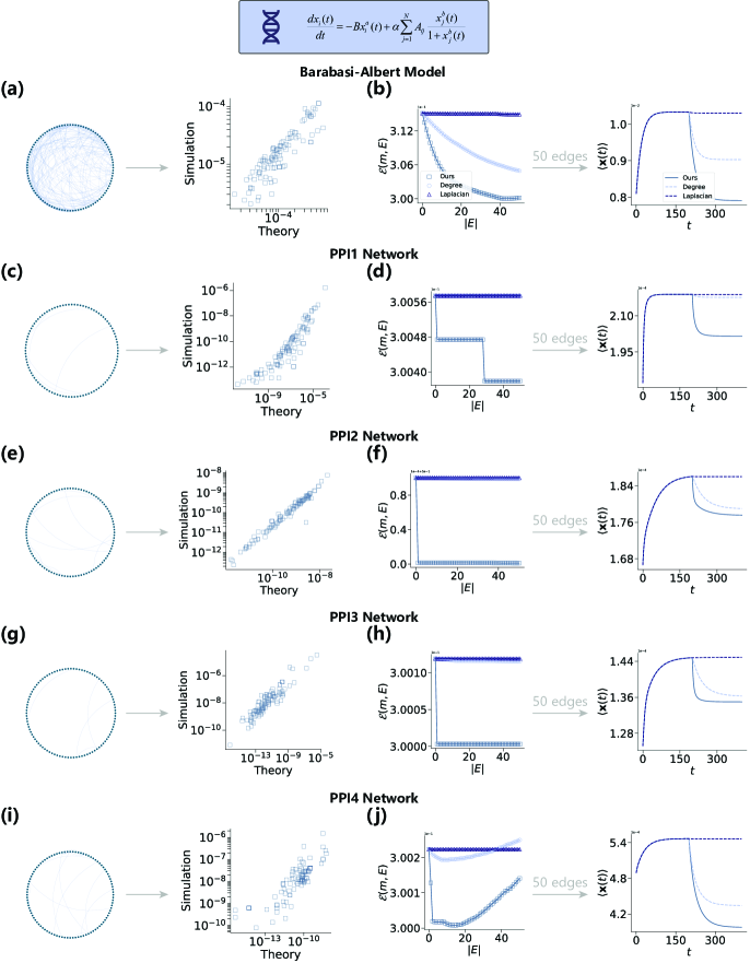
Simulations are preformed on the Barabási-Albert model and four real networks: the first is PPI1(academic name as the protein-protein interaction network of yeast), consisting of 1647 nodes and 5036 edges[56]. The second is PPI2(academic name as the human protein-protein interaction network), consisting of 2035 nodes and 13806 edges[57]. The third is PPI3(academic name as the Arabidopsis thaliana protein-protein interaction network), consisting of 2938 nodes and 7720 edges[58]. The fourth is PPI4(academic name as the Rattus norvegicus gene-protein interaction network), consisting of 2350 nodes and 3484 edges[59]. We removed certain edges in the given protein-protein or gene-protein network and simulated the resulting change in energy . The simulation outcomes are depicted in Figure 7, demonstrating that our theoretical predictions accurately match in the gene network, thereby confirming the validity of our theoretical framework.
5.2 Advice to Gene Regulation
In this section, we continue to utilize edge manipulation to regulate gene expression. We removed specific edges to evaluate the gene expression level and monitor alterations in expression levels. Aligned with our framework, we conducted simulations on the theoretical network and four real networks referenced in Section 5.1. We computed across the edge set and by incorporating the weights of select edges over time , where can indicate variations in gene expression levels. These findings were compared with both degree centrality and Laplacian centrality and are illustrated in Figure 7. It is obvious that our results consistently surpassed the other two centralities in nearly all instances. The enhancement in control with a limited number of edges suggests that our centrality provides a unique advantage in gene regulation.
6 Discussion and Outlook
In this paper, we propose a centrality measure for identifying key motifs in dynamical complex systems. This measure is based on the definition of perturbation energy, which is determined by the elements in the Jacobian matrix. It considers both the topological connections and dynamic properties of the system, revealing the propagation and stability characteristics of the system. Moreover, our centrality only requires the calculation of matrix elements, significantly improving the precision of predicting key motifs without imposing a significant computational burden. To validate our theoretical framework, we conducted simulations on real dynamic systems and integrated them with real world scenarios. Our findings validate the effectiveness and efficiency of our centrality measure for dynamic control, providing significant implications for the formulation of epidemic prevention, ecological protection, gene regulation control, and policies for managing public opinion.
However, our framework is effective for small perturbations and fixed interaction matrices, large perturbations can destabilize the system, making it challenging to accurately estimate system states. Addressing large perturbations necessitates the use of nonlinear dynamics, which requires advanced mathematical tools[60]. Additionally, for time-varying systems where the interaction matrix depends on time , it may be possible to use the Jacobian matrix at a specific moment to replace the matrix in our proposed centrality. However, the implications of this substitution require further exploration and a deeper understanding of time-varying systems.
Declaration of Competing Interest
The authors declare no competing interests.
Acknowledgments
We would like to thank the referees for their constructive comments and suggestions. This work is partly supported by the National Natural Science Foundation of China (Nos.12371354, 12161141003, 11971311) and Science and Technology Commission of Shanghai Municipality, China (No.22JC1403600), National Key R&D Program of China under Grant No. 2022YFA1006400 and the Fundamental Research Funds for the Central Universities, China.
Data Availability
The data and code that support the findings of this study are openly available in GitHub, https://github.com/QitongHu2000/Centrality-Signal-Propagation-data.
Code Availability
The data and code that support the findings of this study are openly available in GitHub, https://github.com/QitongHu2000/Centrality-Signal-Propagation-main.
Appendix A Calculations for Mathematical Equations
A.1 Detailed Proof for Eq.(4)
According to the estimation of proposed in Eq. (3), we use the Sherman-Morrison formula to calculate and consider the limit as approaches 0. In this case, there should be
| (14) | ||||
in which represents the value of matrix on the -th row and -th column, which is equivalent to . Next, we analyze the remaining term in Eq. (3) and consider the fact that . This enables us to derive an accurate estimation for :
| (15) | ||||
By combining Eq. (LABEL:equ:appendix:A1) and Eq. (15), and based on the definitions of and , we can derive . This allows us to obtain the precise expression for :
| (16) | ||||
Finally, taking into account the property , Eq. (3) can be simplified to:
| (17) | ||||
A.2 Detailed Proof for Eq.(6)
In the framework outlined in the main text, we introduce a small perturbation value to a set of edges . This perturbation impacts the Jacobian matrix , where . We have defined the following terms: , , and . Subsequently, we have:
| (18) |
as proposed in the main text, we define and . And we can have:
| (19) | ||||
in which for the second term, we apply the Lagrange mean value theorem with , where and . Therefore, we can approximate and when is very small. Consequently, we can derive the simplified expression for :
| (20) | ||||
References
- [1] B. Barzel, A.-L. Barabási, Universality in network dynamics, Nature physics 9 (2013) 673 – 681.
- [2] U. Harush, B. Barzel, Dynamic patterns of information flow in complex networks, Nature Communications 8 (2017) 2181.
- [3] C. Hens, U. Harush, S. Haber, R. Cohen, B. Barzel, Spatiotemporal signal propagation in complex networks, Nature Physics 15 (2019) 403–412.
- [4] X. Bao, Q. Hu, P. Ji, W. Lin, J. Kurths, J. Nagler, Impact of basic network motifs on the collective response to perturbations, Nature Communications 13 (2022) 5301.
- [5] Q. Hu, X.-D. Zhang, Fundamental patterns of signal propagation in complex networks, Chaos 34 (2024) 013149.
- [6] S. Bontorin, M. D. Domenico, Multi pathways temporal distance unravels the hidden geometry of network-driven processes, Communications Physics 6 (2023) 129.
- [7] V. Thibeault, A. Allard, P. Desrosiers, The low-rank hypothesis of complex systems, Nature Physics (2024) 294–302.
- [8] J. Gao, B. Barzel, A.-L. Barabási, Universal resilience patterns in complex networks, Nature 536 (2016) 238–238.
- [9] C. Ma, G. Korniss, B. K. Szymanski, J. Gao, Universality of noise-induced resilience restoration in spatially-extended ecological systems, Communications Physics 4 (2021) 262.
- [10] H. Zhang, Q. Wang, W. Zhang, S. Havlin, J. Gao, Estimating comparable distances to tipping points across mutualistic systems by scaled recovery rates, Nature Ecology & Evolution 6 (2022) 1524 – 1536.
- [11] C. Meena, C. Hens, S. Acharyya, S. Haber, S. Boccaletti, B. Barzel, Emergent stability in complex network dynamics, Nature Physics 19 (2023) 1033–1042.
- [12] D. Zhao, X. Ling, H. Peng, M. Zhong, J. Han, W. Wang, Robustness of interdependent directed higher-order networks against cascading failures, Physica D 462 (2024) 134126.
- [13] Y.-Y. Liu, J.-J. E. Slotine, A.-L. Barabási, Controllability of complex networks, Nature 473 (2011) 167–173.
- [14] G. Yan, G. Tsekenis, B. Barzel, J.-J. E. Slotine, Y.-Y. Liu, A.-L. Barabási, Spectrum of controlling and observing complex networks, Nature Physics 11 (2015) 779 – 786.
- [15] H. Sanhedrai, J. Gao, A. Bashan, M. Schwartz, S. Havlin, B. Barzel, Reviving a failed network through microscopic interventions, Nature Physics 18 (2020) 338–349.
- [16] H. Sanhedrai, S. Havlin, Sustaining a network by controlling a fraction of nodes, Communications Physics 6 (2022) 1–12.
- [17] R. M. D’Souza, M. di Bernardo, Y.-Y. Liu, Controlling complex networks with complex nodes, Nature Reviews Physics 5 (2023) 250–262.
- [18] C.-L. Yang, C. S. Suh, On controlling dynamic complex networks, Physica D 441 (2022) 133499.
- [19] R. Milo, S. S. Shen-Orr, S. Itzkovitz, N. Kashtan, D. B. Chklovskii, U. Alon, Network motifs: simple building blocks of complex networks, Science 298 (2002) 824–827.
- [20] M. Girvan, M. E. J. Newman, Community structure in social and biological networks, Proceedings of the National Academy of Sciences 99 (2001) 7821 – 7826.
- [21] T. Bröhl, K. Lehnertz, Centrality-based identification of important edges in complex networks, Chaos 29 (2019) 033115.
- [22] L. Lu, D. Chen, X. Ren, Q.-M. Zhang, Y.-C. Zhang, T. Zhou, Vital nodes identification in complex networks, Physics Reports 650 (2016) 1–63.
- [23] H. Liu, X. Xu, J. an Lu, G. Chen, Z. Zeng, Optimizing pinning control of complex dynamical networks based on spectral properties of grounded laplacian matrices, IEEE Transactions on Systems, Man, and Cybernetics: Systems 51 (2018) 786–796.
- [24] G. Bianconi, A. Capocci, Number of loops of size h in growing scale-free networks., Physical review letters 90 (2002) 078701.
- [25] H.-J. Kim, J. M. Kim, Cyclic topology in complex networks., Physical Review E 72 (2005) 036109.
- [26] T. Fan, L. Lü, D. Shi, T. Zhou, Characterizing cycle structure in complex networks, Communications Physics 4 (2020) 272.
- [27] S. Jiang, J. Zhou, M. Small, J. an Lu, Y. Zhang, Searching for key cycles in a complex network., Physical Review Letters 130 (2023) 187402.
- [28] R. Lambiotte, M. Rosvall, I. Scholtes, From networks to optimal higher-order models of complex systems, Nature Physics 15 (2019) 313 – 320.
- [29] F. Battiston, E. Amico, A. Barrat, G. Bianconi, G. F. de Arruda, B. Franceschiello, I. Iacopini, S. Kéfi, V. Latora, Y. Moreno, M. M. Murray, T. P. Peixoto, F. Vaccarino, G. Petri, The physics of higher-order interactions in complex systems, Nature Physics 17 (2021) 1093 – 1098.
- [30] F. Battiston, G. Cencetti, I. Iacopini, V. Latora, M. Lucas, A. Patania, J.-G. Young, G. Petri, Networks beyond pairwise interactions: Structure and dynamics, Physics Reports 874 (2020) 1–92.
- [31] G. St-Onge, H. Sun, A. Allard, L. H’ebert-Dufresne, G. Bianconi, Universal nonlinear infection kernel from heterogeneous exposure on higher-order networks, Physical Review Letters 127 (2021) 158301.
- [32] J. T. Lizier, F. M. Atay, J. Jost, Information storage, loop motifs, and clustered structure in complex networks., Physical Review E 86 (2012) 026110.
- [33] C. Fan, L. Zeng, Y. Sun, Y.-Y. Liu, Finding key players in complex networks through deep reinforcement learning, Nature Machine Intelligence 2 (2020) 317 – 324.
- [34] T. L. I. Diseases, An appropriate response to sars, The Lancet Infectious Diseases 3 (2003) 259 – 259.
- [35] R. P. Wenzel, M. B. Edmond, Listening to sars: Lessons for infection control, Annals of Internal Medicine 139 (2003) 592–593.
- [36] E. Estrada, Covid-19 and sars-cov-2. modeling the present, looking at the future, Physics Reports 869 (2020) 1 – 51.
- [37] M. Chinazzi, J. T. Davis, M. Ajelli, C. Gioannini, M. Litvinova, S. Merler, A. P. y Piontti, K. Mu, L. Rossi, K. Sun, C. G. Viboud, X. Xiong, H. Yu, M. E. Halloran, I. M. Longini, A. Vespignani, The effect of travel restrictions on the spread of the 2019 novel coronavirus (covid-19) outbreak, Science 368 (2020) 395 – 400.
- [38] A. Aleta, Q. Hu, J. Ye, P. Ji, Y. Moreno, A data-driven assessment of early travel restrictions related to the spreading of the novel covid-19 within mainland china, Chaos, Solitons, and Fractals 139 (2020) 110068.
- [39] K. Yagasaki, Nonintegrability of the seir epidemic model, Physica D 453 (2023) 133820.
- [40] S. Liu, M. Y. Li, Epidemic models with discrete state structures, Physica D 422 (2021) 132903.
- [41] Y. Wang, J. Ma, J. Cao, Basic reproduction number for the sir epidemic in degree correlated networks, Physica D 433 (2022) 133183.
- [42] P. S. Dodds, D. J. Watts, A generalized model of social and biological contagion, Journal of Theoretical Biology 232 (2005) 587–604.
- [43] R. A. Rossi, N. K. Ahmed, The network data repository with interactive graph analytics and visualization, in: Proceedings of the Twenty-Ninth AAAI Conference on Artificial Intelligence, AAAI’15, AAAI Press, 2015, p. 4292–4293.
- [44] J. Tang, T. Lou, J. Kleinberg, S. Wu, Transfer link prediction across heterogeneous social networks, ACM Transactions on Information Systems 9 (2010) 1–43.
- [45] T. Opsahl, P. Panzarasa, Clustering in weighted networks, Socity Networks 31 (2009) 155–163.
- [46] J.-P. Eckmann, E. Moses, D. Sergi, Entropy of dialogues creates coherent structures in e-mail traffic, Proceedings of the National Academy of Sciences 101 (2004) 14333–14337.
- [47] P. Massa, M. Salvetti, D. Tomasoni, Bowling alone and trust decline in social network sites, 2009 Eighth IEEE International Conference on Dependable, Autonomic and Secure Computing (2009) 658–663.
- [48] R. May, Simple mathematical models with very complicated dynamics, Nature 261 (1976) 459–467.
- [49] Y. Wang, A. Li, L. Wang, Networked dynamic systems with higher-order interactions: stability versus complexity, National Science Review (2024) nwae103.
- [50] C. S. Holling, Some characteristics of simple types of predation and parasitism, The Canadian Entomologist 91 (1959) 385–398.
- [51] J. C. Marlin, W. E. Laberge, The native bee fauna of carlinville, illinois, revisited after 75 years: a case for persistence, Conservation Ecology 5 (2001) 9.
- [52] U. Alon, An introduction to systems biology : design principles of biological circuits, Chapman and Hall/CRC, 2019.
- [53] G. Karlebach, R. Shamir, Modelling and analysis of gene regulatory networks, Nature Reviews Molecular Cell Biology 9 (2008) 770–780.
- [54] B. Barzel, O. Biham, Binomial moment equations for stochastic reaction systems., Physical Review Letters 106 (2011) 150602.
- [55] R.-J. Wu, Y.-X. Kong, Z. Di, J. Bascompte, G.-Y. Shi, Rigorous criteria for the collapse of nonlinear cooperative networks, Physical Review Letters 130 (2023) 097401.
- [56] H. Yu, P. Braun, M. A. Yildirim, I. Lemmens, et al., High-quality binary protein interaction map of the yeast interactome network, Science 322 (2008) 104 – 110.
- [57] J.-F. Rual, K. Venkatesan, T. Hao, et al., Towards a proteome-scale map of the human protein–protein interaction network, Nature 437 (2005) 1173–1178.
- [58] K. Ikehara, A. Clauset, Characterizing the structural diversity of complex networks across domains, arXiv e-print (2017) abs/1710.11304.
- [59] M. D. Domenico, V. Nicosia, A. Arenas, V. Latora, Structural reducibility of multilayer networks., Nat. Commun. 6 (2015) 6864.
- [60] G. Bianconi, A. Arenas, J. D. Biamonte, L. D. Carr, B. Kahng, J. Kertész, J. Kurths, L. Lü, C. Masoller, A. E. Motter, M. Perc, F. Radicchi, R. Ramaswamy, F. A. Rodrigues, M. Sales-Pardo, M. S. Miguel, S. Thurner, T. Yasseri, Complex systems in the spotlight: next steps after the 2021 nobel prize in physics, Journal of Physics: Complexity 4 (2023) 010201.