A lifted Bregman strategy for training
unfolded proximal neural network Gaussian denoisers

Tóm tắt nội dung

Unfolded proximal neural networks (PNNs) form a family of methods that combines deep learning and proximal optimization approaches. They consist in designing a neural network for a specific task by unrolling a proximal algorithm for a fixed number of iterations, where linearities can be learned from prior training procedure. PNNs have shown to be more robust than traditional deep learning approaches while reaching at least as good performances, in particular in computational imaging. However, training PNNs still depends on the efficiency of available training algorithms. In this work, we propose a lifted training formulation based on Bregman distances for unfolded PNNs. Leveraging the deterministic mini-batch block-coordinate forward-backward method, we design a bespoke computational strategy beyond traditional back-propagation methods for solving the resulting learning problem efficiently. We assess the behaviour of the proposed training approach for PNNs through numerical simulations on image denoising, considering a denoising PNN whose structure is based on dual proximal-gradient iterations.

Index Terms—  Image Gaussian denoising, unfolding, proximal neural networks, Bregman distance

1 Introduction

In the last decade, deep learning approaches have become state-of-the-art in solving a great variety of tasks in data science [1]. In particular, they have shown to be highly successful for solving image restoration problems. In this context, feedforward convolutional neural networks (CNNs) are commonly used, such as celebrated DnCNN [2], Unet [3] and their variations. Such CNNs can be formulated as a composition of operators

$$(\forall x\in\mathbb{R}^{N})\quad G_{\boldsymbol{\theta}}(x)=F_{\theta_{K}}\circ T_{\theta_{K-1}}\cdots\circ T_{\theta_{0}}(x),$$ (1)

where $\boldsymbol{\theta}=(\theta_{k})_{1\leq k\leq K}\in\Theta$ are the underlying parameters of the network (e.g. convolution kernels, biases), $F_{\theta_{K}}\colon\mathbb{R}^{N_{K}}\to\mathbb{R}^{N}$ is an affine function parametrized by $\theta_{K}$ and, for every $k\in\{0,\ldots,K-1\}$,

$$T_{\theta_{k}}\colon\mathbb{R}^{N_{k}}\to\mathbb{R}^{N_{k+1}}\colon u\mapsto D_{k}(F_{\theta_{k}}(u)),$$ (2)

with $F_{\theta_{k}}\colon\mathbb{R}^{N_{k}}\to\mathbb{R}^{N_{k+1}}$ being an affine function parametrized by $\theta_{k}$, and $D_{k}\colon\mathbb{R}^{N_{k+1}}\to\mathbb{R}^{N_{k+1}}$ being an activation function. More recently, inspired by the seminal work of Gregor and Lecun [4] on LISTA, the optimization community started developing unfolded networks based on proximal optimization algorithms, namely proximal neural networks (PNNs). These network architectures basically unroll a fixed number of iterations of proximal algorithms (then renamed layers), where different linear operators can be learned at each layer. Within the formulation (1)-(2), for every $k\in\{0,\ldots,K\}$, $D_{k}$ corresponds to a proximity operator, and $F_{\theta_{k}}$ often corresponds to a gradient step. It has been shown that most of the activation functions used for feedforward networks correspond to proximity operators [5, 6, 7].

On the one hand, PNNs have shown to outperform traditional proximal algorithms, and to reach similar performance as advanced CNNs for image restoration tasks [8, 9]. On the other hand, since their structure is reminiscent of optimization theory, they also gain in interpretability and robustness [10]. Nevertheless, the robustness gained in the network architecture is still limited by the training procedure, as deep neural networks rely on highly parametrized nonlinear systems.

Standard methods for learning parameters $\boldsymbol{\theta}$ (such as SGD and Adam [11]) employ first order optimization methods where the (sub-)gradient information is evaluated using the back-propagation algorithm [12]. Despite its popularity, this standard approach can suffer from potential drawbacks. First, the associated minimization problem is typically non-convex and existing algorithms offer no guarantee of optimality for the delivered output parameters. A second major issue is vanishing and exploding gradients, where gradients become extremely small or large, causing computation challenges, especially for deeper architectures [13]. Finally, the sequential nature of back-propagation makes it difficult to distribute computation for individual partial derivatives across multiple workers, hence constraining the overall training efficiency.

These limitations have inspired fruitful research in seeking alternative training methods [14, 5, 15, 16, 17, 18, 19, 20, 21]. One strategy consists in reformulating the original network parameter estimation problem as a penalized problem that can be solved by distributed optimization methods. In particular, in [21] the lifted Bregman (LB) training strategy has been proposed, that splits the training process over the different layers and associates the proximal activation functions with tailored Bregman distance functions. By construction, the LB formulation leads to a relaxed problem, involving a collection of bi-convex penalty functions, paving the way to the use of advanced optimization algorithms for the parameter estimation. Due to its particular structure that leverages proximity operator theory, the LB approach appears to be particularly well suited for training PNNs. Hence, in this work, we explore a bespoke training procedure for PNNs in the simplified context of image denoising, leveraging the LB approach [21].

The paper is structured as follows. We provide backgrounds on optimization and PNNs in Section 2. In Section 3 we review lifted training strategies, focusing on the LB formulation. We then introduce in Section 4 a LB formulated training strategy for our PNN. In Section 5, we give numerical experiment setups and show the efficiency of the proposed approach for image denoising. We conclude in Section 6.

2 Background

2.1 Notation

We begin this section by first introducing useful definitions. Let $\psi\colon\mathbb{R}^{N}\to]-\infty,+\infty]$ be a proper, lower semi-continuous and convex function. The proximity operator of $\psi$ at $v\in\mathbb{R}^{N}$ is defined as ${\rm prox}_{\psi}(v)=\underset{u\in\mathbb{R}^{N}}{{\rm argmin}}\,\,\psi(u)+\frac{1}{2}\|u-v\|^{2}$. The Fenchel-Legendre conjugate function of $\psi$ at $u\in\mathbb{R}^{N}$ is defined as $\psi^{\ast}(u)=\sup_{x\in\mathbb{R}^{N}}\left\{\langle x,u\rangle-\psi(x)\right\}$. The Bregman penalty function [21] associated with $\psi$ at $(u,v)\in(\mathbb{R}^{N})^{2}$ is defined as

$$B_{\psi}(u,v):=q_{\psi}(u)+q_{\psi}^{\ast}\left(v\right)-\langle u,v\rangle$$ (3)

where $q_{\psi}(u)=\frac{1}{2}\|u\|^{2}+\psi(u)$ and $q_{\psi}^{\ast}$ refers to the Fenchel-Legendre conjugate of $q_{\psi}$ . As a Bregman distance [22, 23], $B_{\psi}(u,v)$ is non-negative and, for $v\in\mathbb{R}^{N}$ fixed, its global minimum value is zero and ${\rm prox}_{\psi}(v)=\underset{u\in\mathbb{R}^{N}}{{\rm argmin}}\,\,B_{\psi}(u,v)$. It is differentiable with respect to its second argument, with

$$(\forall(u,v)\in(\mathbb{R}^{N})^{2})\quad\nabla_{v}B_{\psi}(u,v)={\rm prox}_{\psi}(v)-u.$$ (4)

2.2 Image denoising

An image denoising problem seeks to find an estimate $\widehat{x}\in\mathbb{R}^{N}$ of an original clean image $\overline{x}\in\mathbb{R}^{N}$ from noisy observations $z\in\mathbb{R}^{N}$. We focus on the case of additive Gaussian noise, where the forward model is given by $z=\bar{x}+\epsilon$ where $\epsilon\in\mathbb{R}^{N}$ is a realization of a random zero-mean Gaussian variable with standard deviation $\sigma>0$. A common strategy consists in defining $\widehat{x}$ as

$$\widehat{x}=\underset{x\in\mathbb{R}^{N}}{{\rm argmin}}\,\,\frac{1}{2}\|x-z\|^{2}+g(Lx),$$ (5)

where $g\colon\mathbb{R}^{S}\to\mathbb{R}^{N}$ is some regularization function and $L\colon\mathbb{R}^{N}\to\mathbb{R}^{S}$ is a linear operator [24, 25, 26].

2.3 PNNs for image denoising

Problem (5) can be solved efficiently by the dual forward backward algorithm (dual-FB) [27], given by

$$\begin{array}[]{l}\text{for }k=0,1,\ldots\\ \left\lfloor\begin{array}[]{l}\tau_{k}\in[\underline{\tau},(2-\underline{\tau})\|L\|^{-2}]\\ u_{k+1}={\rm prox}_{\tau_{k}g^{*}}\big{(}u_{k}-\tau_{k}L(L^{*}u_{k}-z)\big{)},\end{array}\right.\end{array}$$ (6)

where $\underline{\tau}>0$. Then, according to [27], we have $\widehat{x}=\lim_{k\to+\infty}z-L^{*}u_{k}$.

Recently, a few works have proposed to unroll the dual-FB algorithm to design unfolded PNNs. In particular, in [28, 29, 30], the authors unrolled the dual-FB algorithm for the denoising problem, and shown that despite having $10^{3}$ less parameters than a DRUnet [31], it reaches similar performances. We hence adopt a similar strategy and unroll algorithm (6) over a fixed number of iterations $K\in\mathbb{N}^{*}$ to construct a composited nonlinear mapping $G_{\boldsymbol{\theta}}$ of the form of (1)-(2) with

$$\begin{cases}T_{\theta_{0}}\colon\mathbb{R}^{N}\to\mathbb{R}^{S}\colon x\mapsto L_{\theta_{0}}x\\ F_{\theta_{K}}\colon\mathbb{R}^{S}\to\mathbb{R}^{N}\colon u\mapsto z-L_{\theta_{K}}^{*}u,\end{cases}$$

and for every $k\in\{1,\ldots,K-1\}$,

$$(\forall u\in\mathbb{R}^{S})\quad T_{\theta_{k}}=\widetilde{T}_{\theta_{k}}^{(\mathcal{D})}\Big{(}\widetilde{T}_{\theta_{k}}^{(\mathcal{P})}(u)\Big{)}$$ (7)

with

$$\widetilde{T}_{\theta_{k}}^{(\mathcal{P})}\!\colon\mathbb{R}^{S}\!\!\to\mathbb{R}^{N}\!\!\times\!\mathbb{R}^{S}\colon u\mapsto\big{(}L_{\theta_{k}}^{*}u+z,\,u\big{)},$$ (8)

$$\widetilde{T}_{\theta_{k}}^{(\mathcal{D})}\!\colon\mathbb{R}^{N}\!\!\!\times\!\mathbb{R}^{S}\!\!\!\to\!\mathbb{R}^{N}\!\colon\!(x,u)\!\mapsto{\rm prox}_{\tau_{k}g^{*}}\!(u-\tau_{k}L_{\theta_{k}}x)$$ (9)

and $\tau_{k}\in[\underline{\tau},(2-\underline{\tau})\|L_{\theta_{k}}\|^{-2}]$. Each intermediate layer is a composition of a proximal activation function over an affine transformation where the underlying parameters of $(T_{\theta_{k}})_{0\leq k\leq K-1}$ and $F_{\theta_{K}}$ are $\boldsymbol{\theta}=(\theta_{k})_{0\leq k\leq K}$, corresponding to a parametrization of the linear operators $(L_{\theta_{k}})_{0\leq k\leq K}$. We define by $\Theta$ the feasible space for $\boldsymbol{\theta}$. In this context, the unfolded network allows the use of different linear operator $L_{\theta_{k}}$ across layers, hence providing higher adaptivity to the task of interest by enlarging the feasibility space.

3 Learning strategies

3.1 Lifted training strategies

In the context of supervised learning for image denoising, we assume that we have access to a training dataset composed of couples of groundtruth/noisy images $(\overline{x}^{(s)},z^{(s)})_{s\in\mathbb{S}}$. Then, standard supervised learning approaches often aim to

$$\underset{\boldsymbol{\theta}\in\Theta}{{\rm minimize}}\,\,\dfrac{1}{\#(\mathbb{S})}\sum_{s\in\mathbb{S}}\ell\Big{(}G_{\boldsymbol{\theta}}(z^{(s)}),\overline{x}^{(s)}\Big{)}\,,$$ (10)

where $\ell\colon\mathbb{R}^{N}\times\mathbb{R}^{N}\to\mathbb{R}$ is a data error function (e.g., $\ell^{2}$ loss) measuring discrepancy between the output of the network $G_{\boldsymbol{\theta}}(z)$ and the groundtruth $\overline{x}$. Standard computational approaches for solving (10) are (sub-)gradient based algorithms (e.g., (sub-)gradient descent or its stochastic variants), where the evaluation of the gradient with respect to $\boldsymbol{\theta}$ is computed using back-propagation [12].

In the context of feedforward networks of the form of (1)-(2), problem (10) can be split over layers by introducing auxiliary dual variables such as, for every $s\in\mathbb{S}$, $u_{0}^{(s)}=T_{\theta_{0}}(z^{(s)})$, $\overline{x}^{(s)}=F_{\theta_{K}}(u_{K-1}^{(s)})$, and, for every $k\in\{1,\ldots,K-1\}$, $u^{(s)}_{k}=T_{\theta_{k}}(u^{(s)}_{k-1})$. Hence, Problem (10) can equivalently be written as a constrained minimization problem:

$$\underset{\boldsymbol{\theta},(\boldsymbol{u}^{(s)})_{s\in\mathbb{S}}}{{\rm minimize}}\,\,\dfrac{1}{\#(\mathbb{S})}\sum_{s\in\mathbb{S}}\ell\Big{(}F_{\theta_{K}}(u_{K-1}^{(s)}),\overline{x}^{(s)}\Big{)}\\ \text{s.t. }\begin{cases}u_{0}^{(s)}=T_{\theta_{0}}(z^{(s)})\\ (\forall k\in\{1,\ldots,K-1\})\;u^{(s)}_{k}=T_{\theta_{k}}(u^{(s)}_{k-1}),\end{cases}$$ (11)

where, for every $s\in\mathbb{S}$, $\boldsymbol{u}^{(s)}=(u_{k}^{(s)})_{0\leq k\leq K-1}$ denotes the auxiliary dual variables for a given pair $(\overline{x}^{(s)},z^{(s)})$. In this equivalent formulation, the popular back-propagation algorithm can be deduced from a Lagrangian formulation [32]. In this context, alternative pathways to standard stochastic back-propagation algorithms can then be considered. Nevertheless, (11) necessitates to handle a collection of non-linear constraints, which can be inefficient in practice.

An approach to overcome this issue is to adopt a penalty approach, where a relaxed formulation of (11) is considered by replacing the constraints by penalty terms [17, 16]. In the next section, we review one such approach that appears to be particularly suited for training PNNs.

3.2 Lifted Bregman approach

Following [21], a relaxed version of problem (11) consists of penalizing the constraints in (11) with penalty functions instead of strictly enforcing them. Here, the penalty functions are chosen as a compositions of the Bregman functions defined in (3) and the affine-linear transformations $F_{\theta_{k}}$. More precisely, we consider the particular case where activation functions $(D_{k})_{0\leq k\leq K-1}$ in (2) are proximity operators of some functions $(\psi_{k})_{0\leq k\leq K-1}$, and $N_{0}=N$ and $N_{1}=\ldots=N_{K}=S$ (i.e., all inner-layers have input/output of the same dimension). This leads to the relaxed formulation

$$\underset{\boldsymbol{\theta},(\boldsymbol{u}^{(s)})_{s\in\mathbb{S}}}{{\rm minimize}}\,\,\dfrac{1}{\#(\mathbb{S})}\bigg{(}\sum_{s\in\mathbb{S}}\ell\big{(}F_{\theta_{K}}(u_{K-1}^{(s)}),\overline{x}^{(s)}\big{)}\\[-5.69046pt] \!+\!B_{\psi_{0}}(u^{(s)}_{0}\!,F_{\theta_{0}}(z^{(s)}))\!+\!\sum_{k=1}^{K-1}\!B_{\psi_{k}}(u^{(s)}_{k},F_{\theta_{k}}(u_{k-1}^{(s)}))\bigg{)}.$$ (12)

The LB approach can be viewed as a generalization of some classical lifted training methods [17, 16]. However, unlike quadratic penalty approaches that still need to differentiate non-smooth activation functions when first-order optimization methods are applied, the Bregman penalty function $B_{\psi}$ is continuously differentiable with respect to its second argument (see (4)), and hence with respect to the network parameters $\boldsymbol{\theta}$. Further, the following properties can be deduced from [21, Theorem 10] (see [21, 33] for more properties).

Proposition 3.1

1. Problem (11) and problem (12) share the same set of solutions.

2. Problem (12) is convex with respect to $\boldsymbol{\theta}$ when $(\boldsymbol{u}^{(s)})_{s\in\mathbb{S}}$ is fixed.

3. For every $k\in\{0,\ldots,K-1\}$, problem (12) is convex with respect to $(\boldsymbol{u}_{k}^{(s)})_{s\in\mathbb{S}}$ when $\boldsymbol{\theta}$ and the other layer’s auxiliary variables are fixed.

The LB training framework fits naturally to the structure of PNNs whose activation functions are proximity operators. In this context, computing the gradient of $B_{\psi}$ with respect to $\boldsymbol{\theta}$ would boil down to using the activation function itself. In the next section, we formulate the LB training problem for the PNN described in Section 2.3.

4 Proposed LB training for PNNs

In this section we design a LB training strategy for the denoising PNN described in Section 2.3.

4.1 Proposed lifted Bregman formulation

One can note that the inner layers of the PNN network described in Section 2.3 are themselves compositions of two feed-forward layers of the form of (2), where the first sub-layers $\widetilde{T}^{(\mathcal{P})}$ (see (8)) provide outputs in $\mathbb{R}^{N}\times\mathbb{R}^{S}$ and the second sub-layers $\widetilde{T}^{(\mathcal{D})}$ (see (9)) take inputs from $\mathbb{R}^{N}\times\mathbb{R}^{S}$. Due to this change of space in the sub-layers, the LB formulation described in Section 3.2 cannot be directly applied, and instead we will need to apply it to the global inner-layers $(T_{\theta_{k}})_{1\leq k\leq K-1}$ defined in (7).

We thus introduce the following LB formulation for our PNN. For the training, we aim to

$$\underset{\boldsymbol{\theta},(\boldsymbol{u}^{(s)})_{s\in\mathbb{S}}}{{\rm minimize}}\,\,\dfrac{1}{\#(\mathbb{S})}\sum_{s\in\mathbb{S}}E\Big{(}\boldsymbol{\theta},\boldsymbol{u}^{(s)}\Big{|}z^{(s)},\overline{x}^{(s)}\Big{)}$$ (13)

where, for any $(\boldsymbol{u},\boldsymbol{\theta})\in(\mathbb{R}^{S})^{K-1}\times\Theta$ and $(\overline{x},z)$, we have

$$E\big{(}\boldsymbol{\theta},\boldsymbol{u}\big{|}z,\overline{x}\big{)}=\ell\big{(}\widetilde{F}_{\theta_{K}}(u_{K-1},z),\overline{x}\big{)}+B_{\tau_{1}g^{*}}\big{(}u_{1},\widetilde{F}_{\theta_{0},\theta_{1}}(z)\big{)}\\ +\sum_{k=2}^{K-1}B_{\tau_{k}g^{*}}\big{(}u_{k},\widetilde{F}_{\theta_{k}}(u_{k-1},z)\big{)}$$ (14)

with

$$\begin{cases}\displaystyle\widetilde{F}_{\theta_{0},\theta_{1}}(z)=({\rm Id}-\tau_{1}L_{\theta_{1}}L_{\theta_{1}}^{*})L_{\theta_{0}}z+\tau_{1}L_{\theta_{1}}z,\\ \displaystyle\widetilde{F}_{\theta_{k}}(u_{k-1},z)=u_{k-1}-\tau_{k}L_{\theta_{k}}(L_{\theta_{k}}^{*}u_{k-1}-z),\\ \widetilde{F}_{\theta_{K}}(u_{K-1},z)=z-L_{\theta_{K}}^{*}u_{K-1}.\end{cases}$$ (15)

In this context, the loss (14) is only convex with respect to the auxiliary variables $(\boldsymbol{u}^{(s)})_{s\in\mathbb{S}}$, but not with respect to the parameters $\boldsymbol{\theta}$, due to the quadratic terms appearing in (15). Nevertheless, Proposition 3.1(ii) still holds in this case.

4.2 Proposed computational strategy

Solving (13)-(14) requires to estimate the network parameters and the auxiliary dual variables. It can be noticed that (14) can be rewritten as the sum of a Lipschitz-differentiable function and a proximable function, i.e., for every $\boldsymbol{u}\in(\mathbb{R}^{S})^{K-1}$, $\boldsymbol{\theta}\in\Theta$ and $(\overline{x},z)\in(\mathbb{R}^{N})^{2}$,

$$E\big{(}\boldsymbol{\theta},\boldsymbol{u}\big{|}z,\overline{x}\big{)}=h(\boldsymbol{u})+f(\boldsymbol{u},\boldsymbol{\theta}|z,\overline{x})$$ (16)

where $h$ is a proximable lower-semicontinuous, proper, convex function, and $f$ is the Lipschitz-differentiable function. In particular, we define $h(\boldsymbol{u})=\sum_{k=1}^{K-1}\tau_{k}g^{*}\big{(}u_{k}\big{)}$, while $f$ contains all the other terms.

Then, we can rely on a block-coordinate forward-backward (FB) strategy to solve (13), alternating between the optimization of $\boldsymbol{\theta}$ and the optimization of the auxiliary variables, whose iterations can be summarized as

$$\begin{array}[]{l}\text{for }n=0,1,\ldots\\ \left\lfloor\begin{array}[]{l}\boldsymbol{\theta}^{(n+1)}=\boldsymbol{\theta}^{(n)}-\beta_{n}\nabla_{\boldsymbol{\theta}}f(\boldsymbol{u}^{(n)},\boldsymbol{\theta}^{(n)}|z)\,,\\ \boldsymbol{u}^{(n+1)}={\rm prox}_{\gamma_{n}\boldsymbol{\tau}g^{*}}\left(\boldsymbol{u}^{(n)}-\gamma_{n}\nabla_{\boldsymbol{u}}f(\boldsymbol{u}^{(n)},\boldsymbol{\theta}^{(n+1)}|z)\right)\end{array}\right.\end{array}$$ (17)

where $\boldsymbol{\tau}=\operatorname{Diag}((\tau_{k})_{1\leq k\leq K-1})$ and, for every $n\in\mathbb{N}$, $(\beta_{n},\gamma_{n})\in]0,+\infty[^{2}$ are step-sizes that must be chosen to ensure convergence of the iterates generated by (17) (see, e.g., [34]). The partial gradients of $f$ in (17) are evaluated using auto-differentiation combined with the differentiation property (4) of the Bregman function. Finally, to use the proposed approach in a training setting, we consider a mini-batch approach in our simulations, where the partial gradients are approximated on sub-parts of the training dataset.

Step-size backtracking strategy.   The choice of step-sizes $(\beta_{n})_{n\in\mathbb{N}}$ and $(\gamma_{n})_{n\in\mathbb{N}}$ in (17) relies on the computation of the Lipschitz constants associated with the gradients of function $f$. In the considered training context, such a computation can be very expensive, and instead we propose a backtracking strategy that relies on monotone properties of the block-coordinate FB algorithm (that holds even for non-convex objective functions). Indeed, according to [34], the step-sizes should be chosen to satisfy, for every $n\in\mathbb{N}$,

$$f(\boldsymbol{u}^{(n)},\boldsymbol{\theta}^{(n+1)}|z)\leq f(\boldsymbol{u}^{(n)},\boldsymbol{\theta}^{(n)}|z)\\ +\langle\boldsymbol{\theta}^{(n+1)}-\boldsymbol{\theta}^{(n)},\nabla_{\boldsymbol{\theta}}f(\boldsymbol{u}^{(n)},\boldsymbol{\theta}^{(n)}|z)\rangle\\ +\frac{1}{2\beta_{n}}\|\boldsymbol{\theta}^{(n+1)}-\boldsymbol{\theta}^{(n)}\|^{2}$$ (18)

and

$$f(\boldsymbol{u}^{(n+1)},\boldsymbol{\theta}^{(n+1)}|z)\leq f(\boldsymbol{u}^{(n)},\boldsymbol{\theta}^{(n+1)}|z)\\ +\langle\boldsymbol{u}^{(n+1)}-\boldsymbol{u}^{(n)},\nabla_{\boldsymbol{u}}f(\boldsymbol{u}^{(n)},\boldsymbol{\theta}^{(n+1)}|z)\rangle\\ +\frac{1}{2\gamma_{n}}\|\boldsymbol{u}^{(n+1)}-\boldsymbol{u}^{(n)}\|^{2}.$$ (19)

Since the partial gradients in (18) and (19) need to be evaluated in the iterations (17), verifying these inequalities appears to have a very low computational cost, that only necessitates extra forward passes to evaluate function $f$. We hence propose to use them to design our backtracking strategy. In particular, since the objective is non-convex, we adopt a two-way backtracking approach (i.e., we automatically either increase or decrease the step-sizes at each iteration) in order to choose the largest step-sizes satisfying the majorant properties.

5 Simulations and Results

In this section, we aim to demonstrate the performance of the proposed strategy on an image denoising example. All numerical results are computed using Pytorch 2.2.2 on NVIDIA GeForce RTX 2080 Ti.

5.1 Experiment setup

Datasets.  For the training groundtruth set, we consider a subset of $1,000$ images randomly selected from the Tiny ImageNet dataset [35], and we use patches of size $32\times 32$. The associated noisy images are generated as, for every $s\in\mathbb{S}$, $z^{(s)}=\bar{x}^{(s)}+\epsilon^{(s)}$, with $\epsilon^{(s)}\in\mathbb{R}^{N}$ being a realization of a zero-mean Gaussian variable with standard deviation $\sigma=0.1$. We then evaluate the resulting networks on $9$ images selected from the BSDS dataset [36].

Network architectures.  We evaluate our training procedure for the PNN defined in Section 2.3 for different network depth $K\in\{5,10,15\}$. For the three cases, we fix the number of features to $16$. We set $\tau_{k}$ at $1.8/\|L_{k}\|^{2}$, where the spectral norm is computed via power iteration following the method proposed in [28]. For all our experiments, the network weights are initialized following the strategy proposed in [37].

Evaluation.  We consider two experiment settings to evaluate the performances of the proposed LB-FB training strategy. For both we use the $\ell^{2}$ loss and run algorithms over $50$ epochs.
Mini-batch stability: We fix the number of layers to $K=5$ and investigate the stability of the proposed alternating FB algorithm when considering a mini-batch approach. We vary the batch size at $\{1,2,5,10,20,50,100\}$ and train the networks on a small collection of $100$ images.
Comparison with SGD: We fix the mini-batch size to saturate memory, vary $K\in\{5,10,15\}$, and compare the proposed LB-FB training approach to a standard stochastic gradient descent approach (SGD) implemented in Pytorch. We run both algorithms on the $1,000$ images. For LB-FB, learning rates $(\beta_{n},\gamma_{n})_{n\in\mathbb{N}}$ are determined via the backtracking strategy. For SGD, the choice of learning rate is made via a grid search over values in the range $[1\times 10^{-6},5\times 10^{-4}]$, where it is chosen empirically such that the training loss value is the lowest.

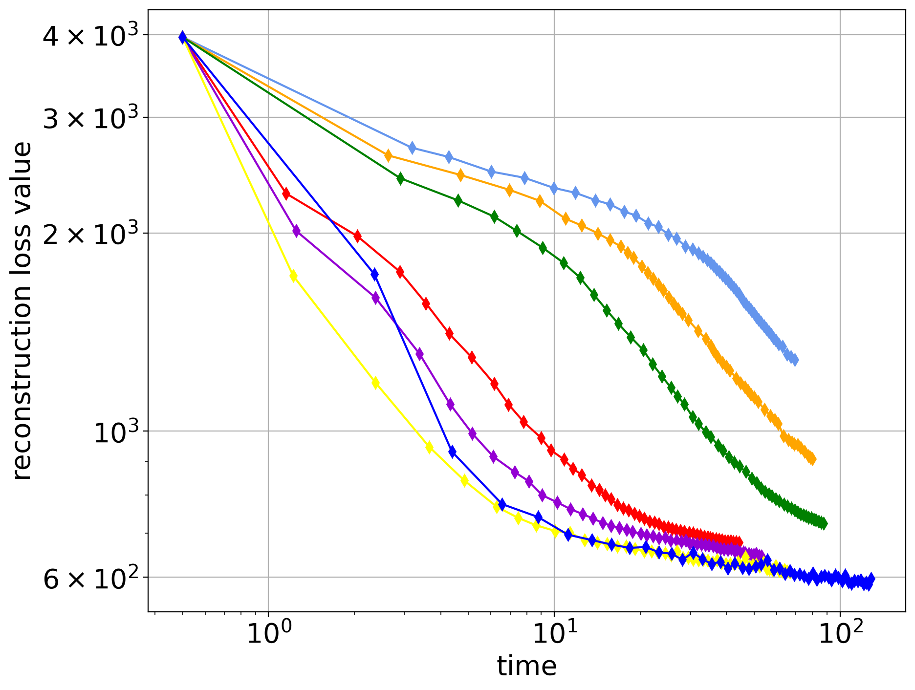
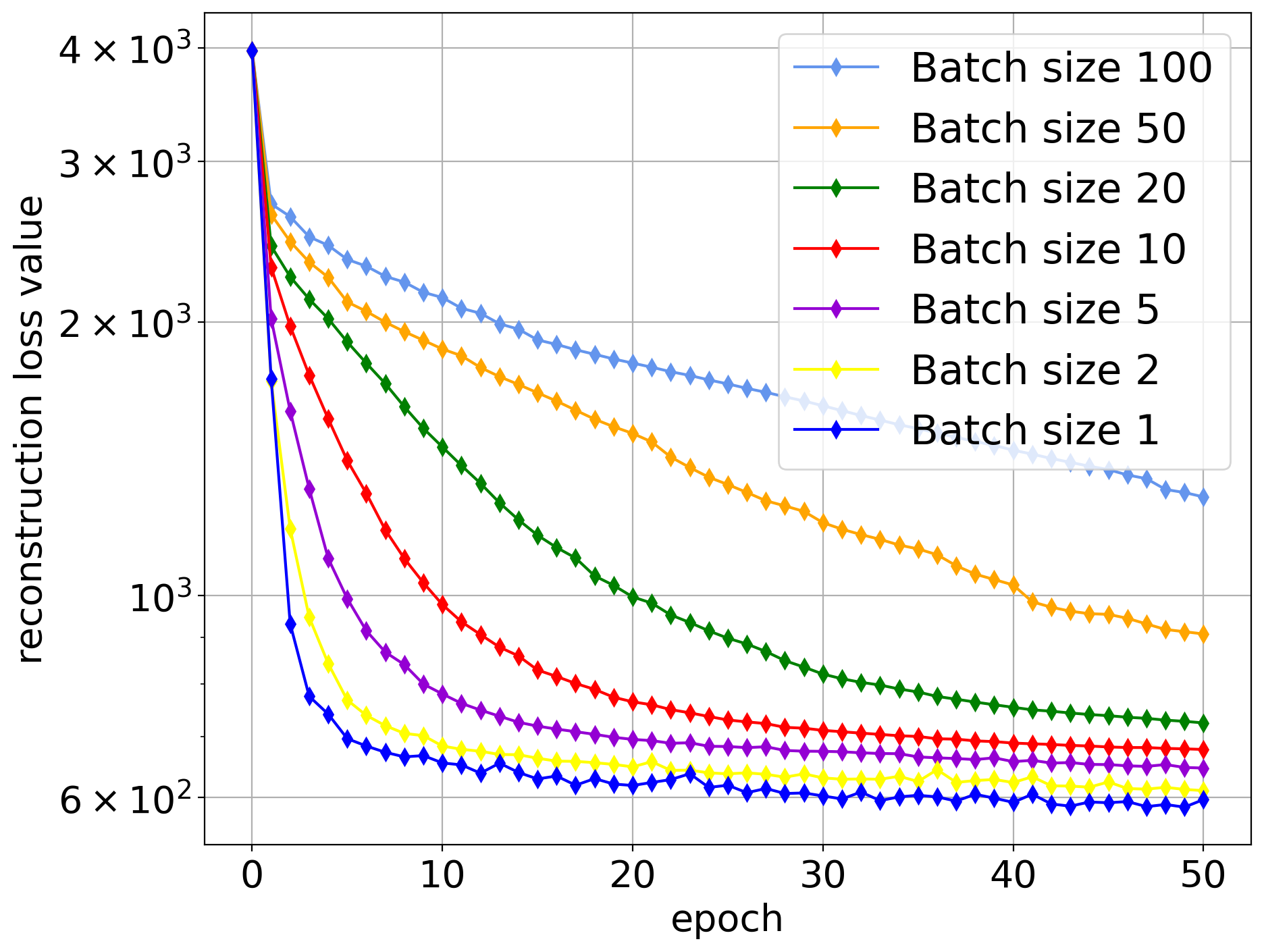
Fig. 1: Mini-batch stability: $\ell^{2}$ loss values with respect to computation time (left) and epochs (right), for different batch sizes.

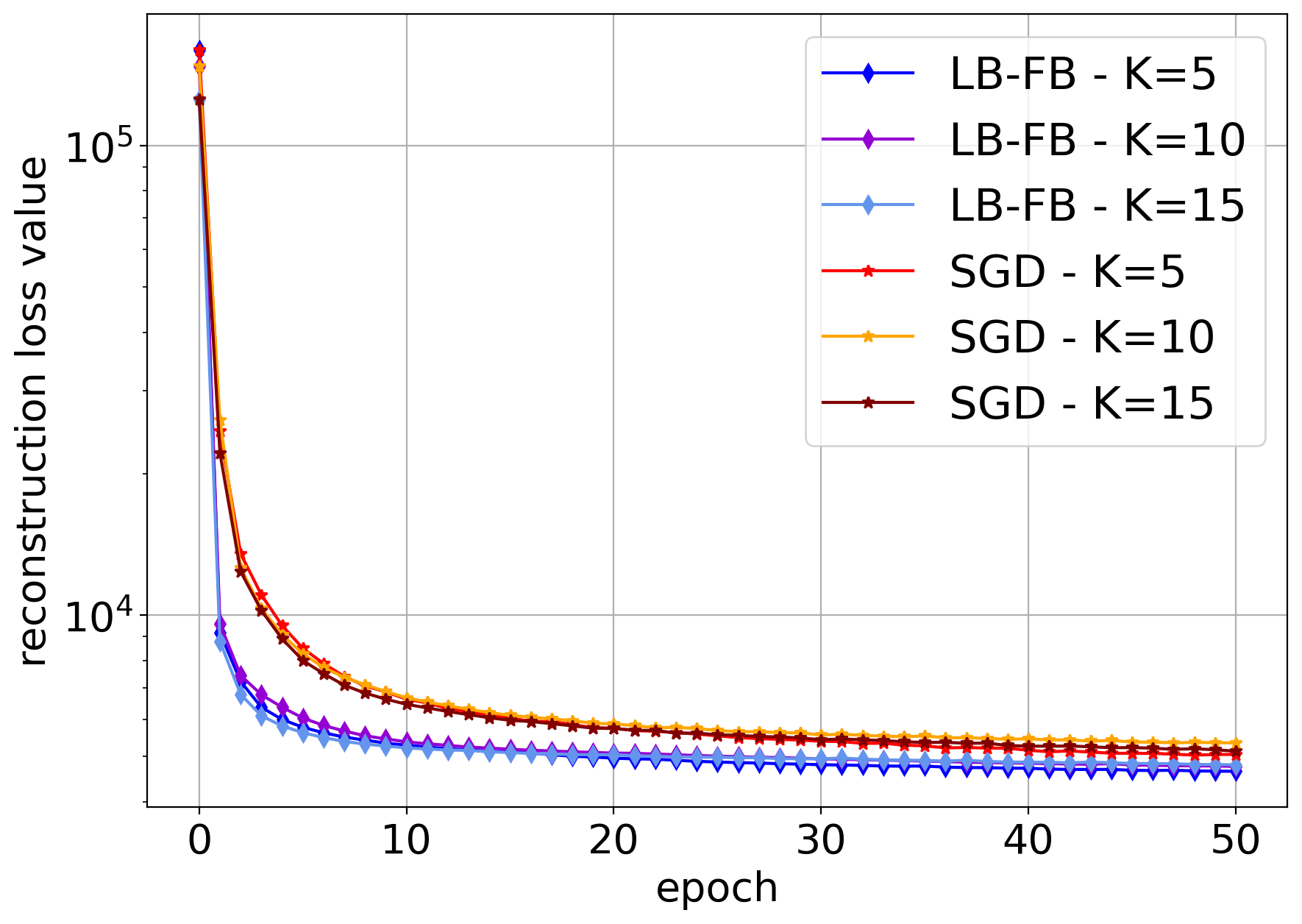
Fig. 2: Comparison with SGD: $\ell^{2}$ loss values comparing with SGD, with respect to computation time (left), and epochs (right).

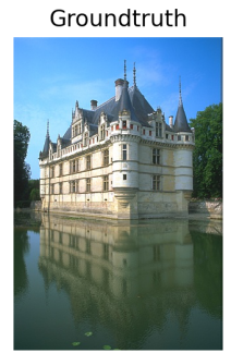
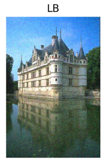
Fig. 3: Denoising results obtained with the proposed LB-FB training strategy on two sample images from the BSDS dataset.

Table 1: Average SSIM and PSNR (and standard deviation) obtained for the $9$ BSDS test images.

	SSIM	PSNR
Noisy	$0.3773\pm 0.0929$	$19.7534\pm 0.3378$
LB-FB	$0.6504\pm 0.0874$	$26.3502\pm 0.4448$
SGD	$0.6413\pm 0.0921$	$26.1366\pm 0.4836$

5.2 Numerical results

Mini-batch stability.  Figure 1 gives the $\ell^{2}$ loss values as defined in Section 4.1 with respect to computational time (left) and epochs (right). On the one hand, we observe that using bigger batch sizes leads to slower convergence. On the other hand, using smaller batch sizes seems to enable better optimization of $\ell^{2}$. However the computation of the $50$ epochs takes longer runtime with very small batch sizes (e.g., $1$ or $2$). Hence a trade-off should be adopted, to avoid saturating the memory while keeping high performances.

Comparison with SGD.  Figure 2 gives the $\ell^{2}$ loss values with respect to epochs, obtained with the proposed LB-FB training approach and with the standard SGD, for the $3$ considered network depths. Overall, we see that LB-FB needs fewer epochs than SGD to converge, and seems more stable (no oscillation ensured by the backtracking approach). We also observe that, as we increase the network depth, a light discrepancy appears between the curves. This suggests that the proposed LB-FB strategy remains stable for deeper network architectures. This is most likely due to the LB formulation, where the training objective is decomposed to layer-wise local objectives.

Finally, for visual inspection, we provide examples of denoised images obtained with our training strategy for $K=15$ in Figure 3. In Table 1 we summarize PSNR and SSIM average scores and standard deviation obtained on the $9$ BSDS test images.

6 Conclusion

In this work, we have proposed a lifted Bregman training strategy combined with a mini-batch block-coordinate forward-backward algorithm for training an unfolded PNN specifically designed for the image Gaussian denoising task. Through numerical experiments, we demonstrated the efficiency of the proposed strategy and showed its competitive performance in training deeper network architectures, comparing to standard SGD approaches using the back-propagation methods.

- [1] I. Goodfellow, Y. Bengio, and A. Courville, Deep Learning. MIT Press, 2016.
- [2] K. Zhang, W. Zuo, Y. Chen, D. Meng, and L. Zhang, “Beyond a gaussian denoiser: Residual learning of deep cnn for image denoising,” IEEE Trans. Image Process., vol. 26, no. 7, pp. 3142–3155, 2017.
- [3] O. Ronneberger, P. Fischer, and T. Brox, “U-net: Convolutional networks for biomedical image segmentation,” in MICCAI 2015, proceedings, part III 18, pp. 234–241, 2015.
- [4] K. Gregor and Y. LeCun, “Learning fast approximations of sparse coding,” in Proc. 27th Int. Conf. Mach. Learn., pp. 399–406, 2010.
- [5] Z. Zhang and M. Brand, “On the convergence of block coordinate descent in training dnns with tikhonov regularization,” in Adv. Neural Inf. Process. Syst., pp. 1719–1728, 2017.
- [6] M. Hasannasab, J. Hertrich, S. Neumayer, G. Plonka, S. Setzer, and G. Steidl, “Parseval proximal neural networks,” J. Fourier Anal. Appl., vol. 26, no. 4, pp. 1–31, 2020.
- [7] P. L. Combettes and J.-C. Pesquet, “Deep neural network structures solving variational inequalities,” Set-Valued Var. Anal., pp. 1–28, 2020.
- [8] J. Adler and O. Öktem, “Learned primal-dual reconstruction,” IEEE Trans. Med. Imaging., vol. 37, no. 6, pp. 1322–1332, 2018.
- [9] M. Jiu and N. Pustelnik, “A deep primal-dual proximal network for image restoration,” IEEE J. Sel. Top. Signal Process., vol. 15, no. 2, pp. 190–203, 2021.
- [10] V. Monga, Y. Li, and Y. C. Eldar, “Algorithm unrolling: Interpretable, efficient deep learning for signal and image processing,” IEEE Sign. Process. Mag., vol. 38, no. 2, pp. 18–44, 2021.
- [11] D. P. Kingma and J. Ba, “Adam: A method for stochastic optimization,” arXiv preprint arXiv:1412.6980, 2014.
- [12] D. E. Rumelhart, G. E. Hinton, and R. J. Williams, “Learning representations by back-propagating errors,” nature, vol. 323, no. 6088, pp. 533–536, 1986.
- [13] K. He, X. Zhang, S. Ren, and J. Sun, “Deep residual learning for image recognition,” in Proc. IEEE Conf. Comput. Vis. Pattern Recognit., pp. 770–778, 2016.
- [14] C. Zach and V. Estellers, “Contrastive learning for lifted networks,” British Machine Vision Conference (BMVC), 2019.
- [15] F. Gu, A. Askari, and L. El Ghaoui, “Fenchel lifted networks: A lagrange relaxation of neural network training,” in Int. Conf. Artif. Intell. Stat., pp. 3362–3371, PMLR, 2020.
- [16] G. Taylor, R. Burmeister, Z. Xu, B. Singh, A. Patel, and T. Goldstein, “Training neural networks without gradients: A scalable admm approach,” in Int. Conf. Mach. Learn., pp. 2722–2731, 2016.
- [17] M. Carreira-Perpinan and W. Wang, “Distributed optimization of deeply nested systems,” in Artificial Intelligence and Statistics, pp. 10–19, PMLR, 2014.
- [18] C. Xu, X. Cheng, and Y. Xie, “An alternative approach to train neural networks using monotone variational inequality,” arXiv preprint arXiv:2202.08876, 2022.
- [19] J. Frecon, G. Gasso, M. Pontil, and S. Salzo, “Bregman neural networks,” in Int. Conf. Mach. Learn., pp. 6779–6792, 2022.
- [20] P. L. Combettes, J.-C. Pesquet, and A. Repetti, “A variational inequality model for learning neural networks,” in Proc. IEEE Int. Conf. Acous. Speech Sig. Process. (ICASSP) 2023, pp. 1–5, 2023.
- [21] X. Wang and M. Benning, “Lifted bregman training of neural networks,” J. Mach. Learn. Res., vol. 24, no. 232, pp. 1–51, 2023.
- [22] L. M. Bregman, “The relaxation method of finding the common point of convex sets and its application to the solution of problems in convex programming,” USSR Comput. Math. Math. Phys., vol. 7, no. 3, pp. 200–217, 1967.
- [23] K. C. Kiwiel, “Proximal minimization methods with generalized bregman functions,” SIAM J. Control Optim., vol. 35, no. 4, pp. 1142–1168, 1997.
- [24] L. I. Rudin, S. Osher, and E. Fatemi, “Nonlinear total variation based noise removal algorithms,” Physica D Nonlinear Phenom., vol. 60, no. 1-4, pp. 259–268, 1992.
- [25] S. Mallat, A wavelet tour of signal processing. Elsevier, 1999.
- [26] L. Jacques, L. Duval, C. Chaux, and G. Peyré, “A panorama on multiscale geometric representations, intertwining spatial, directional and frequency selectivity,” Signal Process., vol. 91, no. 12, pp. 2699–2730, 2011.
- [27] P. L. Combettes, Đ. Dũng, and B. C. Vũ, “Dualization of signal recovery problems,” Set-Valued Var. Anal., vol. 18, no. 3, pp. 373–404, 2010.
- [28] A. Repetti, M. Terris, Y. Wiaux, and J.-C. Pesquet, “Dual forward-backward unfolded network for flexible plug-and-play,” in 30th Eur. Signal Process. Conf. (EUSIPCO), pp. 957–961, 2022.
- [29] H. T. V. Le, N. Pustelnik, and M. Foare, “The faster proximal algorithm, the better unfolded deep learning architecture? the study case of image denoising,” in 30th Eur. Signal Process. Conf. (EUSIPCO), pp. 947–951, 2022.
- [30] H. T. V. Le, A. Repetti, and N. Pustelnik, “Pnn: From proximal algorithms to robust unfolded image denoising networks and plug-and-play methods,” arXiv preprint arXiv:2308.03139, 2023.
- [31] K. Zhang, Y. Li, W. Zuo, L. Zhang, L. Van Gool, and R. Timofte, “Plug-and-play image restoration with deep denoiser prior,” IEEE Transactions on Pattern Analysis and Machine Intelligence, vol. 44, no. 10, pp. 6360–6376, 2021.
- [32] Y. LeCun, D. Touresky, G. Hinton, and T. Sejnowski, “A theoretical framework for back-propagation,” in Proc. 1988 Connect. Models Summer Sch., vol. 1, pp. 21–28, 1988.
- [33] X. Wang and M. Benning, “A lifted bregman formulation for the inversion of deep neural networks,” Front. Appl. Math. Stat., vol. 9, p. 1176850, 2023.
- [34] E. Chouzenoux, J.-C. Pesquet, and A. Repetti, “A block coordinate variable metric forward–backward algorithm,” J. Glob. Optim., vol. 66, no. 3, pp. 457–485, 2016.
- [35] O. Russakovsky, J. Deng, H. Su, J. Krause, S. Satheesh, S. Ma, Z. Huang, A. Karpathy, A. Khosla, M. Bernstein, et al., “Imagenet large scale visual recognition challenge,” Int. J. Comput. Vis., vol. 115, pp. 211–252, 2015.
- [36] D. Martin, C. Fowlkes, D. Tal, and J. Malik, “A database of human segmented natural images and its application to evaluating segmentation algorithms and measuring ecological statistics,” in Proc. 8th IEEE Int. Conf. Comput. Vis., vol. 2, pp. 416–423, 2001.
- [37] X. Glorot and Y. Bengio, “Understanding the difficulty of training deep feedforward neural networks,” in Proc. 13th Int. Conf. Artif. Intell. Stat., pp. 249–256, JMLR Workshop and Conference Proceedings, 2010.