Anisotropic universe with anisotropic dark energy

Abstract

We investigate anisotropic equation of state parameterization of dark energy within the framework of an axisymmetric (planar) Bianchi-I universe. In addition to constraining the equation of state for anisotropic dark energy and other standard cosmological model parameters, we also constrain any underlying anisotropic axis using the latest Pantheon+ Type Ia Supernovae data set augmented by SH0ES Cepheid distance calibrators. The mean anisotropic dark energy equation of state and corresponding difference in the equation of states in and normal to the plane of our axisymmetric Bianchi-I space-time are found to be $\bar{w}=-0.90^{+0.16}_{-0.12}$ and $\delta_{w}=-0.140^{+0.11}_{-0.082}$ respectively. We also find an axis of anisotropy in this planar Bianchi-I model with anisotropic dark energy to be $\approx(279^{\circ},12^{\circ})$ in galactic coordinates. Our analysis of different cosmological models suggests that while a Bianchi-I universe with anisotropic dark energy (the $w_{b}$CDM model) shows some preference over other anisotropic models, it is still less likely than the standard $\Lambda$CDM model or a model with a constant dark energy equation of state ($w$CDM). Overall, the $\Lambda$CDM model remains the most probable model based on the Akaike Information Criterion.

I Introduction

Understanding the nature and behaviour of dark energy stands as one of the most pressing challenges in modern cosmology. While the standard cosmological model, based on the Friedmann-Lemaître-Robertson-Walker (FLRW) metric, has been remarkably successful in explaining a wide range of observational data, it assumes spatial homogeneity and isotropy on large scales of our universe aka the Cosmological principle [1]. However, recent observations indicate a violation of Cosmological principle [2, 3, 4, 5, 6]. In the standard cosmological model viz., the flat $\Lambda$CDM model, dark energy which is responsible for the accelerated expansion of our universe [7] is modeled as a cosmological constant, $\Lambda$, that is an isotropic source with an equation of state given by $w_{\rm de}=-1$ [8, 9]. A potential resolution for the observational hints suggesting deviation from isotropy can be explored via the anisotropic expansion dynamics of our universe [10, 11, 12, 13, 14].

Anisotropic dark energy (ADE) models, which allows for temporal variation (due to their dynamic nature) of the equation of state (e.o.s.) parameter, $w_{\rm de}$, offer a promising avenue for exploring deviations from isotropy and addressing cosmological tensions. In this context, the Bianchi-I universe serves as an immediate generalization for studying spatially homogeneous but anisotropic cosmologies [15, 16, 17, 18, 19, 20]. The axisymmetric nature of the Bianchi-I metric provides sufficient features for investigating the interplay between geometry and energy content, offering insights into the underlying physics driving cosmic evolution.

The Cosmic Microwave Background (CMB) observations [21, 22, 23], although conforms with standard cosmological model based on Cosmological principle, exhibits various anisotropic features at large angular scales which were extensively studied in the literature [24, 25, 26, 27]. Similar studies on statistical violation of isotropy have also been done from the observations of various astronomical data sets such as Type Ia Supernovae [28, 29, 30, 31, 32, 33], Quasars [34, 35, 36, 37, 38], radio polarization vector alignments [39, 40, 41], large scale velocity flows in $\Lambda$CDM cosmology [42], large-scale velocity field from the Cosmicflows-4 data [43]. Interestingly many of these anisotropy axes align with each other broadly in the same direction as the Virgo cluster [44]. In the current era of explosive amounts of data and computation being available readily, the Cosmological principle specifically “statistical isotropy” has been put to test from time to time for its validity. In this context, it would be interesting to test whether the current expansion of our universe is anisotropic i.e., whether ‘cosmological constant’ or another form of dark energy is driving this expansion equally in all directions or not.

To begin with, we require a space-time metric $g_{\mu\nu}$ which can describe global anisotropy that is a solution to Einstien’s field equations but is homogeneous. There exists such family of solutions called ‘Bianchi models’ or ‘homogeneous cosmologies’ [45]. In fact, there has been extensive work done on these anisotropic but homogeneous models [46, 47, 48, 49]. One of the simplest generalizations to standard cosmological model based on FLRW metric is to consider a Bianchi type-I metric that is given by,

$$ds^{2}=c^{2}dt^{2}-a(t)^{2}[dx^{2}+dy^{2}]-b(t)^{2}dz^{2}\,,$$ (1)

where the expansion factors are different in the $x$-$y$ plane ($a(t)$) and the $z$-axis normal to it ($b(t)$). The constant ‘$c$’ in the above metric is the speed of light and is set to unity i.e., $c=1$ for the rest of this paper. They could otherwise be different in different directions, say ‘$a(t)$’ and ‘$b(t)$’ and ‘$c(t)$’ along the three cartesian coordiantes. The form of the Bianchi-I metric we chose above is motivated by different kinds of physical sources with azimuthal symmetry [50, 51, 52]. Such a space-time has come to be known as Eccentric or Ellipsoidal Universe [51, 53].

The anisotropic energy-momentum tensor corresponding to such an axisymmetric metric is taken to be,

$$T^{\mu}_{\nu}={\rm diag}(\rho,-p_{a},-p_{a},-p_{b})\,,$$ (2)

where, $p_{a}$ = $w_{a}\rho$ and $p_{b}$ = $w_{b}\rho$ are the anisotropic pressure terms in the plane normal to and along the anisotropy axis, and $\rho$ is its energy density. We will consider anisotropic dark energy with different equations of state parameterization as a source of anisotropy in this paper.

In section II, we briefly describe the Bianchi-I metric, its Einstein’s field equations, the relationship between distance modulus and redshift within the context of a Bianchi-I space-time, and finally a system of evolution equations (in dimensionless variables) essential for deriving constraints later in our investigation. Following this, we provide a concise overview of the data set utilized in our analysis in section III before presenting our findings and a detailed analysis of constraints obtained in section IV. Lastly, in section V, we discuss the results and conclude.

II Luminosity distance-vs-Redshift relation in a Bianchi-I universe

To constrain the parameters characterizing Bianchi-I model of Eq. (1), we utilize the latest compilation of Type Ia Supernovae (SNIa) data as elaborated in the next section. Here, we introduce the theoretical luminosity distance ($d_{L}$) versus redshift ($z$) relation, which is central to deriving constraints on various cosmological parameters of our model using SNIa data. Additionally, we outline the evolution equations governing these parameters, which must be solved in conjunction with the $d_{L}-z$ relation. For more details, the reader may consult Refs. [15, 16, 54, 55].

We start by defining a mean scale factor and eccentricity parameter (denoting deviation from isotropic expansion) for our Bianchi-I model as,

$$A=(a^{2}b)^{1/3}\quad\text{and}\quad e^{2}=1-\frac{b^{2}}{a^{2}}\,.$$ (3)

These definitions in turn allow us to define average Hubble parameter, and the shear parameter i.e., the differential expansion rate of our universe as,

$$H=(2H_{a}+H_{b})/3\quad{\rm and}\quad\Sigma=(H_{a}-H_{b})/\sqrt{3}\,,$$ (4)

where $H=\dot{A}/A$, $H_{a}=\dot{a}/a$ and $H_{b}=\dot{b}/b$. Here an overdot ($\dot{\hskip 10.00002pt}$) represents derivative with respect to cosmic time ‘$t$’. In terms of these variables, Einstein’s field equations and local conservation of energy-momentum tensor can be found to be given by,

$$\frac{dH}{dt} = -H^{2}-{\frac{2}{3}}\Sigma^{2}-{\frac{1}{6}}(\rho+2p_{a}+p_{b})\,,$$

$$\frac{d\Sigma}{dt} = -3H\Sigma+\frac{1}{\sqrt{3}}(p_{a}-p_{b})\,,$$ (5)

$$\frac{d\rho}{dt} = -3H(\rho+\frac{2p_{a}+p_{b}}{3})-\frac{2\Sigma}{\sqrt{3}}(p_{a}-p_{b})\,,$$

along with the constraint equation,

$$H^{2}=\frac{\rho}{3}+\frac{\Sigma^{2}}{3}\,.$$ (6)

Using the above constraint equation, we can define the dimensionless energy density parameter $\Omega=\rho/(3H^{2})$ (in units of $c=8\pi G=1$) and the expansion-normalized dimensionless shear parameter $\sigma=\Sigma/(\sqrt{3}H)$. It is important to note that the energy density $\rho$ in Eq. (6), and consequently $\Omega$, comprises two components : the isotropic (ordinary and dark) matter denoted by ‘$\Omega_{m}$’, and the anisotropic dark energy denoted by ‘$\Omega_{\rm ade}$’. By defining the critical energy density as $\rho_{c,0}$ or simply $\rho_{0}=3H^{2}_{0}$, where $H_{0}$ represents the current value of the mean Hubble parameter (i.e., $H(t_{0})=H_{0}$), we can express the constraint equation at present as,

$$\Omega_{m,0}+\Omega_{\rm ade,0}+\sigma^{2}_{0}=1\,,$$ (7)

where $\Omega_{m,0}=\rho_{m,0}/\rho_{0}$ and $\Omega_{\rm ade,0}=\rho_{\rm ade,0}/\rho_{0}$ that represent the fractional energy densities due to respective sources as indicated at the current time ‘$t_{0}$’. Hereafter, we will omit the subscript ‘$0$’ for brevity, denoting them simply as $\Omega_{m}$ and $\Omega_{\rm ade}$. However, their usage should be clear from the context, whether they refer to energy densities at the current time or time-dependent variables. Finally, we define a dimensionless time variable as $\tau=\ln(A)$, leading to $H=d\tau/dt$.

The relation between direction-dependent luminosity distance ($d_{L}$) and redshift ($z$) of a Type Ia Supernova object observed in the direction $\hat{n}=(\theta,\phi$) in a Bianchi-I universe is given by [15],

$$d_{L}(\hat{n})=c(1+z_{\rm hel})\int_{A(z^{*})}^{1}\frac{dA}{{A^{2}}H}\frac{(1-e^{2})^{1/6}}{(1-e^{2}\cos^{2}\alpha)^{1/2}}\,.$$ (8)

Here, $\alpha=\cos^{-1}(\hat{\lambda}\cdot\hat{n})$ represents the angle between the cosmic preferred axis $\hat{\lambda}$’ (i.e., the $z$-axis of Eq. (1)) and the location of a Type Ia Supernova at ‘$\hat{n}$’ in the sky. Further, ‘$z_{\rm hel}$’ and ‘$z^{*}$’ denotes redshift of a Type Ia Supernova in heliocentric and cosmic (CMB) frames respectively [56].

To solve for the integral in the above expression for luminosity distance ‘$d_{L}$’, one must alongside solve the complete set of evolution equations that are setup in terms of various dimensionless variables defined earlier, following Einstein’s field equations and others. They can be found to be [54, 55],

$$\frac{h^{\prime}}{h} = -\frac{3}{2}(1+\sigma^{2}+\bar{w}\Omega_{\rm ade})\,,$$

$$(e^{2})^{\prime} = 6\sigma(1-e^{2})\,,$$

$$\sigma^{\prime} = -\frac{3}{2}[\sigma(1-\sigma^{2})-(\frac{2}{3}\delta_{w}+\bar{w}\sigma)\Omega_{\rm ade}]\,,$$ (9)

$$\Omega_{\rm ade}^{\prime} = -3\Omega_{\rm ade}(\bar{w}+\frac{2}{3}{\delta_{w}}\sigma-\bar{w}\Omega_{\rm ade}-\sigma^{2})\,,$$

$$\Omega_{m}^{\prime} = 3\Omega_{m}(\bar{w}\Omega_{\rm ade}+\sigma^{2})\,.$$

Here, $\bar{w}$ denotes average equation of state parameter given by $\bar{w}=(2w_{a}+w_{b})/3$, and their difference as $\delta_{w}=w_{a}-w_{b}$. The parameter ‘$h$’ in the preceding equations stands for the dimensionless Hubble parameter in units of $100~{}\text{km/s/Mpc}$ i.e., $h=H/(100~{}\text{km/s/Mpc})$. Finally, for any of the parameters in the evolution equations given above, say $\theta$, a derivative with respect to dimensionless time variable ‘$\tau$’ is denoted by $\theta^{\prime}$.

Thus the cosmological parameters to be constrained in our model are $\{h_{0},e^{2}_{0},\sigma_{0},\Omega_{\rm ade},\Omega_{m},\hat{\lambda}=(l_{a},b_{a})\}$ along with $w_{a}$ and $w_{b}$, or equivalently $\bar{w}$ and $\delta_{w}$. We consider three cases of anisotropic equation of state parameterization for the dark energy as described below :

Case-I

‘$w_{a}$’ as free parameter, and $w_{b}=-1$ (fixed),

Case-II

$w_{a}=-1$ (fixed), and ‘$w_{b}$’ as free parameter,

Case-III

Both $\bar{w}$ and $\delta_{w}$ as free parameters.

Following the constraint equation of Eq. (7), $\Omega_{m}$ is treated as derived parameter, while $\Omega_{\rm ade}$ and $\sigma_{0}$ are varied freely to obtain constraints. Further, the cosmic anisotropy axis in our model, denoted by $\hat{\lambda}=(l_{a},b_{a})$, will be estimated in galactic coordinates.

We compare our results with the standard flat $\Lambda$CDM model, for which the luminosity distance in given by,

$$d_{L}=\frac{c(1+z_{\rm hel})}{H_{0}}\int_{0}^{z^{*}}{\frac{dz}{\sqrt{\Omega_{m}(1+z)^{3}+\Omega_{\Lambda}}}}\,,$$ (10)

where $\Omega_{m}$ represents the current fraction of matter density (comprising dust-like dark+visible matter) in the universe, and $\Omega_{\Lambda}$ is the dark energy density fraction. The constraint equation relating these two parameters at current times is $\Omega_{m}+\Omega_{\Lambda}=1$. Hence, within the standard concordance model, we have two cosmological parameters to be constrained: $H_{0}$ (or equivalently $h_{0}$) and $\Omega_{\Lambda}$ (treating $\Omega_{m}$ as a derived parameter i.e., $\Omega_{m}=1-\Omega_{\Lambda}$), with SNIa absolute magnitude $M_{0}$ remaining as a nuisance parameter. This standard model serves as our reference for comparison with rest of the models that we study here.

As an extension to the flat $\Lambda$CDM model, we also obtain constraints on the $w$CDM model in which the luminosity distance is given by,

$$d_{L}=\frac{c(1+z_{\rm hel})}{H_{0}}\int_{0}^{z^{*}}{\frac{dz}{\sqrt{\Omega_{m}(1+z)^{3}+\Omega_{\rm de}(1+z)^{\beta}}}}\,,$$ (11)

where $\beta=3(1+w_{\rm de})$ and $w_{\rm de}$ is the dark energy equation of state that could be different from ‘$-1$’. Our parameter set in this case is $\{h_{0},\Omega_{\rm de},w_{\rm de},M_{0}\}$ i.e., we choose to constrain $\Omega_{\rm de}$ and the dust-like (dark+visible) matter density fraction will then be given by $\Omega_{m}=1-\Omega_{\rm de}$ following the first Friedmann equation in a flat FLRW space-time.

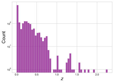
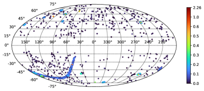
Figure 1: Top : Number count histogram of SNIa in Pantheon+ data with respect to redshift in 100 bins. Bottom : Sky distribution of Pantheon+ SNIa.

III Data set and Likelihood analysis

The Pantheon+ compilation of Type Ia Supernovae (SNIa) comprises of 1701 light curves in turn containing approximately 1550 unique spectroscopically confirmed SNIa [57]. We note that the light curves of the remaining SNIa, i.e., those SNIa other than the approximately 1550 out of 1701, are either same Supernova (SN) observed by different surveys or are what are called “SN siblings” that stands for SNIa found in the same host galaxy. Notable enhancements in the latest data set include the addition of new SNIa especially at low redshifts, as well as adjustments for peculiar velocity and host galaxy bias in the SNIa covariance matrix [57]. The redshift and spatial (sky) distribution of SNIa in Pantheon+ compilation are shown in the top and bottom panels of Fig. [1] respectively.

Now, we outline the likelihood function ($\mathcal{L}$), that depends on various fitting parameters, including the cosmological parameters under investigation. Using an MCMC method, we maximize the likelihood function by sampling different parameters that it depends on.

Central to deriving constraints on various (cosmological) parameters of interest using SNIa is the theoretical relation between redshift ($z^{*}$) and the luminosity distance ($d_{L}$) that depends on different cosmological parameters via the distance modulus ($\mu^{\rm th}$) that is given by,

$$\mu^{\rm th}=5\log_{10}\left(\frac{d_{L}({\bm{\theta}},z^{*})}{10~{}\text{pc}}\right)=m_{B,\rm corr}-M_{0}\,.$$ (12)

Here, $m_{B,\rm corr}$ represents the (stretch, color, etc.,) corrected apparent $B$-band magnitude of an SNIa, while $M_{0}$ (a global free parameter in our model fitting) denotes the absolute magnitude of an SNIa. Notably, $M_{0}$ exhibits a strong degeneracy with the Hubble parameter $H_{0}$ and is pivotal in motivating the utilization of SH0ES Cepheid variables [58]. Conventionally, ‘$M_{0}$’ is assumed to be same for all SNIa, and we follow the same here also.

Our $\chi^{2}({\bm{\theta}})$ function ($=-\ln(\mathcal{L}(\bm{\theta}))$) that depends on the collective fitting parameters ‘${\bm{\theta}}$’ is defined as,

$$\chi^{2}({\bm{\theta}})=\Delta{\bm{\mu}}^{T}({{\bf C}_{\rm stat+sys}^{\rm SN}+{\bf C}_{\rm stat+sys}^{\rm Cepheid}})^{-1}\Delta{\bm{\mu}}\,,$$ (13)

which is minimized to obtain relevant constraints. Here, $\Delta{\bf\mu}=(\Delta\mu_{1},\Delta\mu_{2},\ldots,\Delta\mu_{n})^{T}$ is a column vector of size $1\times n$ and ‘$n$’ is the number of SNIa in the data set we are using. Then the residual $\Delta\mu_{i}=\mu^{\rm obs}_{i}-\mu^{\rm th}_{i}$ for an $i$th SNIa is defined as,

$$\Delta\mu_{i}=\hskip 200.0003pt$$ (14)

$$\left\{\begin{array}[]{l l}m^{i}_{B,\rm corr}-M_{0}-\mu_{i}^{\rm Cepheid},&\text{if }i\in\text{Ceph. hosts}\,,\\ m^{i}_{B,\rm corr}-M_{0}-\mu^{\rm th}({\bm{\theta}},z^{*}_{i}),&\text{otherwise}\,.\end{array}\right.$$ (17)

Here $\mu^{\rm obs}_{i}=m^{i}_{B,\rm corr}-M_{0}$, and $\mu^{\rm th}_{i}=\mu^{\rm th}({\bm{\theta}},z^{*}_{i})$ is the theoretical distance modulus that depends on model parameters being constrained and $z^{*}_{i}$ is the redshift of that Supernova. For any SNIa whose host galaxy also contains a Cepheid variable, $\mu^{\rm th}_{i}$ is taken to be the $\mu_{i}^{\rm Cepheid}$. Both $m^{i}_{B,\rm corr}$ and $\mu_{i}^{\rm Cepheid}$ are provided as part of Pantheon+ data release. Considering the correlations between SNIa that are calibrated simultaneously due to both statistical and systematic uncertainties in SNIa light curve fitting, we also use the full covariance matrix. ${\bf C}_{\rm stat+sys}^{\rm SN}$ denotes the SN covariance matrix and ${\bf C}_{\rm stat+sys}^{\rm Cepheid}$ contains the SH0ES Cepheid host-distance covariance matrix, both of which are provided as part of Pantheon+ data set.

Constraints will be derived for the three cases I, II and III of anisotropic equation of state parameterization as described in the previous section. We also obtain constraints on $w$CDM model for completeness. They are then compared with the standard flat $\Lambda$CDM model taking it as base (reference) model.

IV Results

IV.1 Cosmological constraints

We discuss the results obtained from cosmological parameter fitting of Bianchi-I model for our universe with anisotropic dark energy in this section. For the Case-I, $w_{b}=-1$ is fixed i.e., equation of state for dark energy along the anisotropy axis is fixed and the total free parameters during the MCMC fitting are $\{h_{0},M_{0},e^{2}_{0},\sigma_{0},\Omega_{\rm ade},w_{a},(l_{a},b_{a})\}$. For the Case-II, $w_{a}=-1$ is fixed i.e., equation of state for dark energy in the plane normal to the axis of anisotropy is fixed and the free parameters are now $\{h_{0},M_{0},e^{2}_{0},\sigma_{0},\Omega_{\rm ade},w_{b},(l_{a},b_{a})\}$. For the Case-III, both the parameters $\bar{w}=(2w_{a}+w_{b})/3$ and $\delta_{w}=w_{a}-w_{b}$ are kept as free parameters. Hence the total free parameters in Case-III are $\{h_{0},M_{0},e^{2}_{0},\sigma_{0},\Omega_{\rm ade},\bar{w},\delta_{w},(l_{a},b_{a})\}$. Note that the fractional matter density $\Omega_{m}$ in all these three cases is a derived parameter following Eq. (7).

In Fig. [2], we present two-dimensional contour plots illustrating the $1\sigma$ and $2\sigma$ confidence levels (CL) for various cosmological parameters of Case-I and Case-II, specifically ${h_{0},e^{2}_{0},\sigma_{0},\Omega_{\rm ade}}$ and the corresponding respective anisotropic dark energy equation of state parameter. In Fig. [3], similar plots are presented but for the Case-III.

For the $\Lambda$CDM and $w$CDM models, free parameters are $\{h_{0},M_{0},\Omega_{\Lambda}\}$ and $\{h_{0},M_{0},\Omega_{\rm ade},w\}$ respectively. $1\sigma$ and $2\sigma$ confidence levels (CL) for these parameters, specifically $h_{0}$, $\Omega_{\Lambda}$ or $\Omega_{\rm de}$, and $w$, are shown in the corner plot of Fig. [4] in the left and right panels respectively. Here also, following the respective constraint equations involving energy density fractions, we constrain $\Omega_{\Lambda}$ or $\Omega_{\rm de}$ as a free parameter thus calculating $\Omega_{m}$ as a derived parameter.

For all models that we studied, the posterior distributions of $\Omega_{m}$ (top left), $M_{0}$ (top right), and also $\bar{w}$ and $\delta_{w}$ (bottom panels for easy comparison with base model) are presented in Fig. [5]. The vertical lines in the bottom panels correspond to $\bar{w}=-1$ and $\delta_{w}=0$ as expected in the standard flat $\Lambda$CDM model. All the parameter constraints for the five models viz., three cases of anisotropic dark energy in axisymmetric Bianchi-I universe (Case-I, II and III) and the $\Lambda$CDM and $w$CDM models are presented in Table 1.

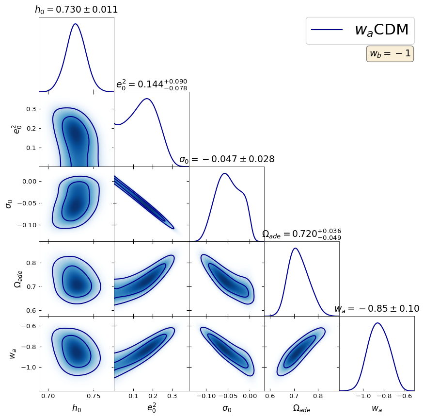
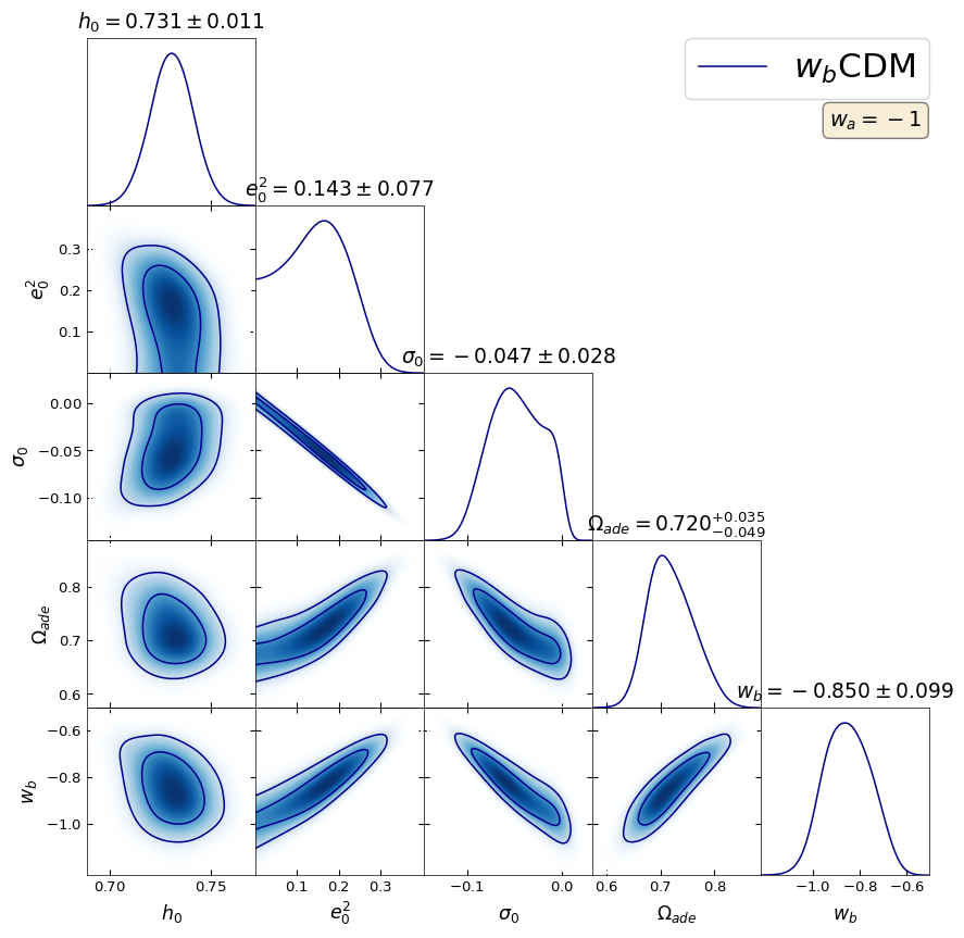
Figure 2: Parameter constraints with 1$\sigma$ and 2$\sigma$ CL for all free parameters in two cases of anisotropic equation of state parameterization of dark energy in the residual plane of symmetry (Case-I:$w_{a}$CDM, top) and normal to that plane (Case-II:$w_{b}$CDM, bottom) as source of anisotropy in an axisymmetric Bianchi-I model.

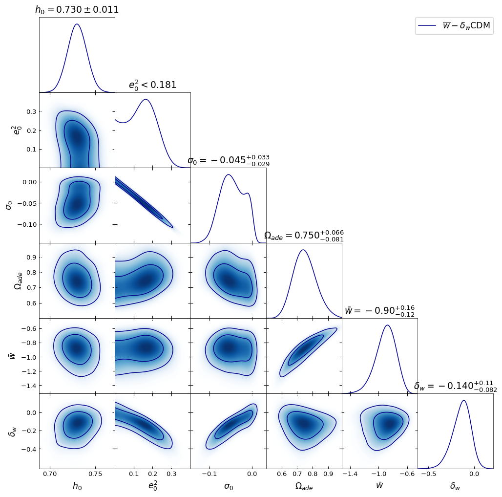
Figure 3: 2D confidence contours of all cosmological parameters in Case-III of our axisymmetric Bianchi-I model with anisotropic dark energy whose equation of states along the cosmic $z$-axis ($w_{a}$) and in the plane normal to it ($w_{a}$) are freely varied. The actual equation of state parameters constrained are the mean equation of state of anisotropic dark energy, $\bar{w}=(2w_{a}+w_{b})/3$, and the difference in the two equations of state $\delta_{w}=w_{a}-w_{b}$ that captures anisotropic expansion of dark energy in different directions.

The likelihood contour plots indicate that the anisotropic dark energy density we examined in the first two cases i.e., $w_{a}$CDM and $w_{b}$CDM models are: $\Omega_{\rm ade}=0.720^{+0.036}_{-0.049}$ and $0.720^{+0.035}_{-0.049}$ respectively, which is slightly lower than that found in Case-III i.e., the $\bar{w}-\delta_{w}$CDM model: $\Omega_{\rm ade}=0.750^{+0.066}_{-0.081}$. Similarly, the constraints on present-day cosmic shear for $w_{a}$CDM and $w_{b}$CDM model are: $\sigma_{0}=-0.047\pm{0.028}$ in both models, which we slightly lower than the cosmic shear found in Case-III: $\sigma_{0}=-0.045^{+0.033}_{-0.029}$. However, we should perhaps not read too much into these differences in parameter estimates from among the three cases as they are consistent with each other within errorbars (see Table 1). It is important to note that the estimated cosmic shear parameter, $\sigma_{0}$, is preferring a negative value in all the three cases. For the anisotropic dark energy fraction in all three cases, we find that they are in agreement with each other: $\Omega_{\rm ade}\approx 0.720$, and in turn with the isotropic $w$CDM model: $\Omega_{\rm de}=0.721^{+0.056}_{-0.082}$. However, these values are significantly higher than the base $\Lambda$CDM model: $\Omega_{\Lambda}=0.666\pm{0.018}$.

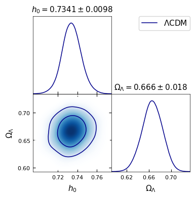
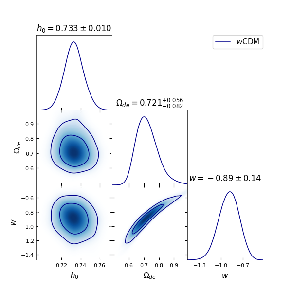
Figure 4: 1$\sigma$ and 2$\sigma$ confidence contour plots of various cosmological parameters in our base $\Lambda$CDM(left), and the $w$CDM (right) cosmological model.

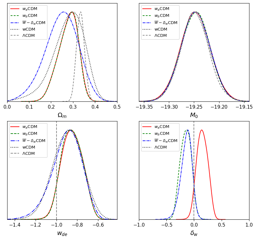
Figure 5: Posterior distribution of isotropic matter $\Omega_{m}$ (top left), absolute B-band magnitude of Type Ia Supernova (top right), various dark energy equation of state parameters ($w_{\rm ade}$/$w_{\rm de}$), and the difference in dark energy equation of state $\delta_{w}=w_{a}-w_{b}$ for all cases of Bianchi-I model as well as $\Lambda$CDM and $w$CDM models.

Given the fit for non-zero cosmic shear from SNIa data in the three cases of $w_{a}$CDM, $w_{b}$CDM, and $\bar{w}-\delta_{w}$CDM, we may infer that the cosmic expansion is perhaps different in different directions. Consequently, we anticipate similar constraints on the eccentricity parameter ($e_{0}^{2}$) as is the case with $\sigma_{0}$. We do find that the eccentricity parameter is non-zero and further consistent between $w_{a}$CDM and $w_{b}$CDM models: $e^{2}_{0}=0.144^{+0.090}_{-0.078}$ and $0.143\pm{0.077}$ respectively, while we only get an upper bound in the case of $\bar{w}-\delta_{w}$CDM model: $e^{2}_{0}<0.181$. This indicates that $a_{0}=b_{0}=1$, meaning that their relative scaling is not different from ‘1’ at current times when considering $\bar{w}-\delta_{w}$CDM model.

Parameter	Case I ($w_{a}$CDM)	Case II ($w_{b}$CDM)	Case III ($\bar{w}-\delta_{w}$CDM)	$\Lambda$CDM	$w$CDM
$h_{0}$	$0.730\pm 0.011$	$0.731\pm 0.011$	$0.730\pm 0.011$	$0.735\pm{0.010}$	$0.733\pm{0.010}$
$\sigma_{0}$	$-0.047\pm{0.028}$	$-0.047\pm{0.028}$	$-0.045^{+0.033}_{-0.029}$	-	-
$e^{2}_{0}$	$0.144^{+0.090}_{-0.078}$	$0.143\pm{0.077}$	$<0.181$	-	-
$\Omega_{\rm de}$	$0.720^{+0.036}_{-0.049}$	$0.720^{+0.035}_{-0.049}$	$0.750^{+0.066}_{-0.081}$	$0.666\pm{0.018}$	$0.721^{+0.056}_{-0.082}$
${}^{*}\Omega_{m}$	$0.277^{+0.052}_{-0.037}$	$0.277^{+0.052}_{-0.036}$	$0.247^{+0.082}_{-0.068}$	$0.334\pm 0.018$	$0.279^{+0.082}_{-0.056}$
$\bar{w}$ / $w_{\rm de}$	$-0.950\pm 0.033^{*}$	$-0.950\pm 0.033^{*}$	$-0.90^{+0.16}_{-0.12}$	-1 (fixed)	$-0.89\pm{0.14}$
$\delta_{w}$	$0.15\pm 0.10^{*}$	$-0.150\pm 0.099^{*}$	$-0.140^{+0.11}_{-0.082}$	-	-
$w_{a}$	$-0.85\pm 0.10$	$-1$ (fixed)	$-0.95^{+0.17*}_{-0.13}$	-	-
$w_{b}$	$-1$ (fixed)	$-0.850\pm 0.099$	$-0.81^{+0.17*}_{-0.11}$	-	-
$\hat{\lambda}=(l_{a},b_{a})$	$(281^{+7.7}_{-15},12^{+11}_{-12})$	$(281.3^{+8.3}_{-14},12^{+10}_{-12})$	$(278\pm{13},15.3^{+7.3}_{-15})$	-	-
$M_{0}$	$-19.247\pm 0.030$	$-19.247\pm 0.029$	$-19.247\pm 0.029$	$-19.247\pm{0.029}$	$-19.248\pm{0.030}$
$k$	8	8	9	3	4
$\chi^{2}$	1520	1519.8	1520.3	1525.3	1525.9
$\Delta\chi^{2}$	5.3	5.5	5	0	0.6
$\Delta$	4.7	4.5	7	0	2.6
AICrel	0.095	0.105	0.030	1	0.273

Table 1: Best fit values of all the cosmological parameters of anisotropic Bianchi-I model with three different anisotropic dark energy equation of state parameterizations, including the axes of anisotropy ‘$\hat{\lambda}$’ in galactic coordinates, and the goodness-of-parameters are tabulated here. Here ‘$k$’ dentotes the number of model paramters. ^∗Derived parameters.

One of the most interesting results from this work is constraints on cosmic preferred axis due to anisotropic expansion of the universe which, for all three cases, almost aligns in the same direction. The constraints on the anisotropy axis in all three cases of Bianchi-I model with anisotropic dark energy e.o.s. are: $(l_{a},b_{a})\approx(281^{\circ},12^{\circ})$, $(281^{\circ},12^{\circ})$ and $(278^{\circ},15^{\circ})$ respectively in galactic coordinates. These axes are shown in Fig. [6] along with their $1\sigma$ confidence contours. Since all these axes are very close by with nearly same errorbars, to avoid clutter in plotting, we show the anisotropy axis with $1\sigma$ CL from $\bar{w}-\delta_{w}$CDM model only. More interestingly it aligns with the preferred axis found in our previous work [55] where anisotropic matter sources were assumed instead of anisotropic dark energy, specifically when cosmic strings (CS) and magnetic fields (MF) were taken to be the source of anisotropy. There we found that the anisotropy axis in case of CS and MF are: $(l_{a},b_{a})\approx(290^{\circ},9^{\circ})$ and $(290^{\circ},10^{\circ})$ respectively. The anisotropy axes found here are depicted alongside notable anisotropy axes seen in various data sets, such as CMB, radio data, SNIa, the CMB dipole ($\ell=1$), etc., as mentioned in the caption of Fig. [6]. It is important to note that in the previous work [55], current energy density fractions for these two sources, namely cosmic strings and magnetic fields, were consistent with zero. However we cannot say whether this indicates a systematic in the data that is being picked up by the anisotropic parameterization of dark energy as source in an anisotropic background space-time.

For the anisotropic dark energy equation of state parameter, we get $w_{a}=-0.85\pm 0.10$ and $w_{b}=-0.850\pm 0.099$ for the first two cases of $w_{a}$CDM and $w_{b}$CDM, while we get $\bar{w}=-0.90^{+0.16}_{-0.12}$ and $\delta_{w}=-0.140^{+0.11}_{-0.082}$ for the third case of $\bar{w}-\delta_{w}$CDM. All of these results are shown separately in the bottom panels of Fig. [5] for easy comparison with that of $\Lambda$CDM and $w$CDM models. The equation of state for dark energy (cosmological constant) in the base $\Lambda$CDM model where $w_{\rm de}=-1$ and $\delta_{w}=0$ are also depicted in those two bottom panels as vertical grey lines. We also have additional parameter $\delta_{w}$ in the Case-III which is the difference between equation of state parameters in and normal to the plane of axisymmetry i.e $\delta_{w}=w_{a}-w_{b}=-0.140^{+0.11}_{-0.082}$. Note that in the bottom left panel of Fig. [5], for the first two cases either $w_{b}$ or $w_{a}$ was fixed to ‘$-1$’ while $w_{a}$ and $w_{b}$ were varied. But, it is still interesting that the mean value of this parameter from likelihood maximization is preferring a different value from $\delta_{w}=0$ unlike what is expected based on standard flat $\Lambda$CDM model.

Finally, we also display constraints on the SNIa absolute magnitude ‘$M_{0}$’ in the top right panel of Fig. [5]. As is obvious from the plot, it is essentially same for all models that we studied which is $M_{0}\approx-19.247\pm{0.029}$ and is in agreement with the value originally reported by Pantheon+ collaboration [57]. These values are also listed in Table 1.

IV.2 Goodness of fit

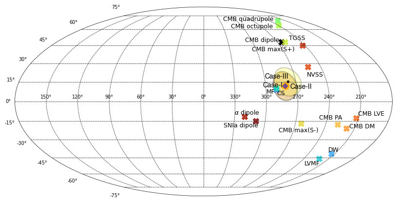
Figure 6: Mollweide projection of the cosmic preferred axis, with $1\sigma$ confidence contours, found using Pantheon+ SNIa data for the three cases of anisotropic equation of state parameterization of dark energy. Also shown are similar axis of anisotropy found in various astronomical/cosmological data : CMB dipole [23], CMB quadrupole and octopole axes [25], CMB Even and odd mirror parity axes, Hemispherical Power Asymmetry (HPA) axis, Dipole Modulation axis [26], CMB HPA axis from Local Variance estimator [59], Radio dipole in NVSS and TGSS data [60], Fine structure constant ($\alpha$) and SNIa Dipole [61], and Cosmic strings, Domain walls, Magnetic fields and Lorentz Violation generated magnetic fields (LVMF) as sources of anisotropy [55].

In assessing the goodness of fit for different models, comparing those with varying number of fit parameters can pose challenges both qualitatively and quantitatively. One straightforward method involves comparing the differences in the minima of the $\chi^{2}$ values between two models, with one serving as the base model, and also computing the $\chi^{2}$ per degree of freedom. For the models studied in the present work, the differences $\Delta\chi^{2}=\chi^{2}_{\rm ref}-\chi^{2}_{\rm model}$ relative to the reference flat $\Lambda$CDM model are presented in third row from the bottom of Table 1.

Expanding the parameter space to describe observed data typically results lower $\chi^{2}$ values at its minima ($\chi^{2}_{\rm min}$). Therefore, a more effective approach to identifying the most suitable model for the observed data should account for the additional parameters introduced during model fitting relative to a base model. One commonly used model selection criterion, derived from information theory, is the Akaike Information Criterion (AIC). Alongside the minimum of $\chi^{2}=-\ln(\mathcal{L})$, where $\mathcal{L}$ represents the likelihood function of the model, the AIC formula incorporates an additional penalty term dependent on the number of parameters ‘$k$’ that were used to fit the data. It is given by [62],

$${\rm AIC}=2k-2\ln(\mathcal{L_{\rm max}})=2k+\chi^{2}_{\rm min}\,.$$ (18)

Here, $\chi^{2}_{\rm min}$ represents the minimum $\chi^{2}$ value attained in the parameter space after optimization of Eq. (13). Relative AIC values for the candidate models are then calculated using one of the models as a reference or base model. This provides an estimate of the probability of the other models in effectively describing the observed data relative to the chosen reference model. It is expressed as,

$${\rm AIC}_{\rm rel}=\exp\left(-\Delta/2\right)\,,$$ (19)

where $\Delta$ in the above expression is the difference between AIC values of a model with respect to a reference model that is given by,

$$\Delta={\rm AIC}_{\rm Bianchi-I}-{\rm AIC}_{\Lambda\rm CDM}\,.$$ (20)

$\Delta$	Strength of Evidence
$\leq 2$	Strong support
4 - 7	Less support
$\geq$ 10	No support

Table 2: Strength of evidence in support of a model ‘$i$’ based on the difference in AIC values: $\Delta_{i}={\rm AIC}_{i}-{\rm AIC}_{\rm min}$, where ${\rm AIC}_{\rm min}$ is the AIC of the model with lowest AIC value from among the candidate models being studied [63].

In our analysis, flat $\Lambda$CDM model serves as base model for comparing the anisotropic Bianchi-I model with anisotropic dark energy, and also the $w$CDM model. The difference in AICs and relative AIC values, $\Delta$ and ${\rm AIC}_{\rm rel}$ respectively, compared to standard concordance model are listed at the end of Table 1. The ${\rm AIC}_{\rm rel}$ values provide a means for model selection indicating how probable various models are under study in comparison to the chosen base model (taken to be ‘1’ i.e., the most probable model to describe our data). Likewise the difference in AIC values, $\Delta$, also enable us in gauging how well a particular candidate model is supported vis-a-vis the reference model. They are given in Table 2 [63].

Our analysis reveals that the Bianchi-I universe with anisotropic dark energy as source of anisotropy in $w_{b}$CDM model is favored over the other two anisotropic cases viz., $w_{a}$CDM and $\bar{w}-\delta_{w}$CDM. However, the relative AIC values suggest that the $w_{b}$CDM model itself is relatively less probable compared to the standard cosmological model or the $w$CDM model. We also note that, the relative AIC values for $w_{a}$CDM and $w_{b}$CDM are very near, and consequently we cannot definitively conclude which anisotropic model provides a better fit to the data between these two.

In light of the interpretation provided by AIC for model selection [62, 63], the flat $\Lambda$CDM model is $\approx$10.5, 9.5, 33, and 2.7 times more probable than $w_{a}$CDM, $w_{b}$CDM, $\bar{w}-\delta_{w}$CDM and $w$CDM models respectively. If we employ a cut-off ${\rm AIC}_{\rm rel}$ value of $\alpha_{\rm AIC}=0.01$ for assessing a specific model i.e., a candidate model being $1\%$ probable relative to the base model, then all the anisotropic Bianchi-I cases and the $w$CDM model remain as potential possibilities. However with a cut-off of $\alpha_{\rm AIC}=0.05$ i.e., a particular model being $\leq 20$ times less likely, then the one with the most free parameters viz., $\bar{w}-\delta_{w}$CDM model has to be excluded from further consideration.

V Conclusions

In this study, assuming a Bianchi-I universe, our aim was to estimate the level of anisotropy in the observed universe by evaluating the anisotropy parameters cosmic shear and eccentricity, constraining the density fractions of (isotropic dark and visible) matter and anisotropic dark energy, and identifying any cosmic preferred axis for our universe. The Bianchi-I model we examined is an anisotropic cosmological model with a residual planar symmetry in the spatial part of its metric. We rederived the evolution equations for various cosmological parameters of this model in the form of coupled differential equations. Subsequently, we performed an MCMC likelihood analysis of the Bianchi-I model, while solving for these evolution equations alongside the corresponding luminosity distance vs. redshift relation by defining a $\chi^{2}$ function. For this analysis, we utilized the latest compilation of Type Ia Supernova (SNIa) data from the Pantheon+ collaboration.

The Hubble parameter value ($h_{0}$) derived from our Bianchi-I model analysis with three different anisotropic dark energy equation of state parameterizations (Case-I, II and III listed in Sec. II) agree with the value from Pantheon+ collaboration [57], and does not alleviate the ‘Hubble tension’ problem.

There is an indication of a negative cosmic shear and a non-zero eccentricity at the present epoch. Cosmic shear constraints indicate that our universe may be expanding mildly anisotropically.

The cosmic anisotropy axes identified in this study in all three cases agree with each other. All three axes found here are also consistent with the axis of anisotropy found in an earlier work [55] for the same Bianchi-I model but with cosmic strings and magnetic fields as sources of anisotropy.

Interestingly, the constratints obtained on equation of state for dark energy in all the three cases of anisotropic Bianchi-I background, and in the $w$CDM model i.e., $w_{\rm ade}$ or $w_{\rm de}$, are preferring a larger value than ‘$-1$’ that is inline with the recent findings from DESI collaboration [64]. We should however note that we didnt consider a dark energy scenario with an evolving equation state.So, this coincidence may be due to the additional parameter freedom in the anisotropic cosmological model that we studied.

When evaluating the evidence for a specific model/anisotropic source that likely describes the data better than the standard concordance model, we find that a flat $\Lambda$CDM model still remains preferable. However, a Bianchi-I model with dark energy as source of anisotropy may warrant further consideration as it is not entirely negated by the AIC metric that we used to assess suitability of different models considered here in fitting the data well. The AIC values of various candidate models indicate that they are either less likely or bordering no support. This could also be a result of the limited constraining power of the SNIa sample used. Although Pantheon+ compilation contains the largest number of Type Ia Supernovae that are simultaneously calibrated available in the public domain, many of the SNIa that are new to the Pantheon+ sample compared to the previous Pantheon SNIa sample are mostly at low redshifts. Therefore, we conclude that more data, especially at intermediate and high redshifts, may enable us to establish stringent constraints and make definitive conclusions regarding these alternative anisotropic models.

References

- [1] Steven Weinberg. Gravitation and Cosmology: Principles and Applications of the General Theory of Relativity. John Wiley and Sons, New York, 1972.
- [2] Dominik J. Schwarz, Craig J. Copi, Dragan Huterer, and Glenn D. Starkman. CMB anomalies after Planck. Classical and Quantum Gravity, 33(18):184001, September 2016.
- [3] Philip Bull et al. Beyond CDM: Problems, solutions, and the road ahead. Phys. Dark Univ., 12:56–99, 2016.
- [4] L. Perivolaropoulos and F. Skara. Challenges for CDM: An update. New A Rev., 95:101659, December 2022.
- [5] Elcio Abdalla et al. Cosmology intertwined: A review of the particle physics, astrophysics, and cosmology associated with the cosmological tensions and anomalies. JHEAp, 34:49–211, 2022.
- [6] Pavan Kumar Aluri et al. Is the observable Universe consistent with the cosmological principle? Class. Quant. Grav., 40(9):094001, 2023.
- [7] S. Perlmutter et al. Measurements of and from 42 High-Redshift Supernovae. Astrophys. J., 517:565–586, 1999.
- [8] D. N. Spergel et al. First year Wilkinson Microwave Anisotropy Probe (WMAP) observations: Determination of cosmological parameters. Astrophys. J. Suppl., 148:175–194, 2003.
- [9] N. Aghanim et al. Planck 2018 results. VI. Cosmological parameters. Astron. Astrophys., 641:A6, 2020. [Erratum: Astron.Astrophys. 652, C4 (2021)].
- [10] T. R. Jaffe, A. J. Banday, H. K. Eriksen, K. M. Górski, and F. K. Hansen. Evidence of Vorticity and Shear at Large Angular Scales in the WMAP Data: A Violation of Cosmological Isotropy? ApJ, 629(1):L1–L4, August 2005.
- [11] Andrew Pontzen. Rogues’ gallery: The full freedom of the Bianchi CMB anomalies. Phys. Rev. D, 79(10):103518, May 2009.
- [12] Rockhee Sung and Peter Coles. Temperature and polarization patterns in anisotropic cosmologies. J. Cosmology Astropart. Phys, 2011(6):036, June 2011.
- [13] Daniela Saadeh, Stephen M. Feeney, Andrew Pontzen, Hiranya V. Peiris, and Jason D. McEwen. A framework for testing isotropy with the cosmic microwave background. MNRAS, 462(2):1802–1811, October 2016.
- [14] Pablo Fosalba and Enrique Gaztañaga. Explaining cosmological anisotropy: evidence for causal horizons from CMB data. MNRAS, 504(4):5840–5862, July 2021.
- [15] Tomi Koivisto and David F. Mota. Anisotropic dark energy: dynamics of the background and perturbations. J. Cosmology Astropart. Phys, 2008(6):018, June 2008.
- [16] L. Campanelli, P. Cea, G. L. Fogli, and A. Marrone. Testing the isotropy of the Universe with type Ia supernovae. Phys. Rev. D, 83(10):103503, May 2011.
- [17] Stephen A. Appleby and Eric V. Linder. Probing dark energy anisotropy. Phys. Rev. D, 87(2):023532, January 2013.
- [18] J. S. Wang and F. Y. Wang. Probing the anisotropic expansion from supernovae and GRBs in a model-independent way. MNRAS, 443(2):1680–1687, September 2014.
- [19] Anil Kumar Yadav, Avinash K. Yadav, Manvinder Singh, Rajendra Prasad, Nafis Ahmad, and Kangujam Priyokumar Singh. Constraining a bulk viscous Bianchi type I dark energy dominated universe with recent observational data. Phys. Rev. D, 104(6):064044, September 2021.
- [20] W. Rahman, R. Trotta, S. S. Boruah, M. J. Hudson, and D. A. van Dyk. New constraints on anisotropic expansion from supernovae Type Ia. MNRAS, 514(1):139–163, July 2022.
- [21] C. L. Bennett, A. J. Banday, K. M. Gorski, G. Hinshaw, P. Jackson, P. Keegstra, A. Kogut, G. F. Smoot, D. T. Wilkinson, and E. L. Wright. Four-Year COBE DMR Cosmic Microwave Background Observations: Maps and Basic Results. ApJ, 464:L1, June 1996.
- [22] C. L. Bennett et al. Nine-Year Wilkinson Microwave Anisotropy Probe (WMAP) Observations: Final Maps and Results. Astrophys. J. Suppl., 208:20, 2013.
- [23] N. Aghanim et al. Planck 2018 results. I. Overview and the cosmological legacy of Planck. Astron. Astrophys., 641:A1, 2020.
- [24] C. L. Bennett et al. Seven-Year Wilkinson Microwave Anisotropy Probe (WMAP) Observations: Are There Cosmic Microwave Background Anomalies? Astrophys. J. Suppl., 192:17, 2011.
- [25] P. A. R. Ade et al. Planck 2013 results. XXIII. Isotropy and statistics of the CMB. Astron. Astrophys., 571:A23, 2014.
- [26] P. A. R. Ade et al. Planck 2015 results. XVI. Isotropy and statistics of the CMB. Astron. Astrophys., 594:A16, 2016.
- [27] Y. Akrami et al. Planck 2018 results. VII. Isotropy and Statistics of the CMB. Astron. Astrophys., 641:A7, 2020.
- [28] D. J. Schwarz and B. Weinhorst. (An)isotropy of the Hubble diagram: comparing hemispheres. A&A, 474(3):717–729, November 2007.
- [29] I. Antoniou and L. Perivolaropoulos. Searching for a cosmological preferred axis: Union2 data analysis and comparison with other probes. J. Cosmology Astropart. Phys, 2010(12):012, December 2010.
- [30] Jacques Colin, Roya Mohayaee, Subir Sarkar, and Arman Shafieloo. Probing the anisotropic local Universe and beyond with SNe Ia data. MNRAS, 414(1):264–271, June 2011.
- [31] David L. Wiltshire, Peter R. Smale, Teppo Mattsson, and Richard Watkins. Hubble flow variance and the cosmic rest frame. Phys. Rev. D, 88(8):083529, October 2013.
- [32] Stephen Appleby, Arman Shafieloo, and Andrew Johnson. Probing Bulk Flow with Nearby SNe Ia Data. ApJ, 801(2):76, March 2015.
- [33] Dong Zhao, Yong Zhou, and Zhe Chang. Anisotropy of the Universe via the Pantheon supernovae sample revisited. MNRAS, 486(4):5679–5689, July 2019.
- [34] D. Hutsemekers. Evidence for very large-scale coherent orientations of quasar polarization vectors. A&A, 332:410–428, April 1998.
- [35] D. Hutsemékers and H. Lamy. Confirmation of the existence of coherent orientations of quasar polarization vectors on cosmological scales. A&A, 367:381–387, February 2001.
- [36] Pankaj Jain, Gaurav Narain, and S. Sarala. Large-scale alignment of optical polarizations from distant QSOs using coordinate-invariant statistics. MNRAS, 347(2):394–402, January 2004.
- [37] D. Hutsemékers, L. Braibant, V. Pelgrims, and D. Sluse. Alignment of quasar polarizations with large-scale structures. A&A, 572:A18, December 2014.
- [38] Nathan J. Secrest, Sebastian von Hausegger, Mohamed Rameez, Roya Mohayaee, Subir Sarkar, and Jacques Colin. A Test of the Cosmological Principle with Quasars. ApJ, 908(2):L51, February 2021.
- [39] P. Birch. Is the Universe rotating? Nature, 298(5873):451–454, July 1982.
- [40] Pankaj Jain and John P. Ralston. Anisotropy in the Propagation of Radio Polarizations from Cosmologically Distant Galaxies. Modern Physics Letters A, 14(6):417–432, January 1999.
- [41] Prabhakar Tiwari and Pankaj Jain. Polarization Alignment in Jvas/class Flat Spectrum Radio Surveys. International Journal of Modern Physics D, 22(12):1350089, October 2013.
- [42] Richard Watkins, Hume A. Feldman, and Michael J. Hudson. Consistently large cosmic flows on scales of 100h-1Mpc: a challenge for the standard CDM cosmology. MNRAS, 392(2):743–756, January 2009.
- [43] Yehuda Hoffman, Aurelien Valade, Noam I. Libeskind, Jenny G. Sorce, R. Brent Tully, Simon Pfeifer, Stefan Gottlöber, and Daniel Pomarède. The large-scale velocity field from the Cosmicflows-4 data. MNRAS, 527(2):3788–3805, January 2024.
- [44] John P. Ralston and Pankaj Jain. The Virgo Alignment Puzzle in Propagation of Radiation on Cosmological Scales. International Journal of Modern Physics D, 13(9):1857–1877, January 2004.
- [45] M. A. H. MacCallum and G. F. R. Ellis. A class of homogeneous cosmological models: II. Observations. Communications in Mathematical Physics, 19(1):31–64, March 1970.
- [46] Michael P. Ryan and Lawrence C. Shepley. Homogeneous Relativistic Cosmologies. Princeton Series in Physics. Princeton University Press, Princeton, 1975.
- [47] J. Wainwright and G. F. R. Ellis. Dynamical Systems in Cosmology. Cambridge Univ. Press, Cambridge, 1997.
- [48] Hans Stephani, Dietrich Kramer, Malcolm MacCallum, Cornelius Hoenselaers, and Eduard Herlt. Exact solutions of Einstein’s field equations. Cambridge Monographs on Mathematical Physics. Cambridge Univ. Press, Cambridge, 2003.
- [49] A. A. Coley. Dynamical systems and cosmology. Astrophysics and Space Science Library. Kluwer Academic Publishers, Dordrecht, Netherlands, 2003.
- [50] John D. Barrow. Cosmological limits on slightly skew stresses. Phys. Rev. D, 55(12):7451–7460, June 1997.
- [51] Arjun Berera, Roman V. Buniy, and Thomas W. Kephart. The eccentric universe. J. Cosmology Astropart. Phys, 2004(10):016, October 2004.
- [52] Leonardo Campanelli. Model of universe anisotropization. Phys. Rev. D, 80(6):063006, September 2009.
- [53] L. Campanelli, P. Cea, and L. Tedesco. Ellipsoidal Universe Can Solve the Cosmic Microwave Background Quadrupole Problem. Phys. Rev. Lett., 97(13):131302, September 2006.
- [54] Pavan K. Aluri, Sukanta Panda, Manabendra Sharma, and Snigdha Thakur. Anisotropic universe with anisotropic sources. J. Cosmology Astropart. Phys, 2013(12):003, December 2013.
- [55] Anshul Verma, Sanjeet K. Patel, Pavan K. Aluri, Sukanta Panda, and David F. Mota. Constraints on Bianchi-I type universe with SH0ES anchored Pantheon+ SNIa data. J. Cosmology Astropart. Phys, 2024(6):071, June 2024.
- [56] Tamara M. Davis et al. The Effect of Peculiar Velocities on Supernova Cosmology. Astrophys. J., 741:67, 2011.
- [57] Dan Scolnic et al. The Pantheon+ Analysis: The Full Data Set and Light-curve Release. Astrophys. J., 938(2):113, 2022.
- [58] Adam G. Riess et al. A Comprehensive Measurement of the Local Value of the Hubble Constant with 1 km s-1 Mpc-1 Uncertainty from the Hubble Space Telescope and the SH0ES Team. Astrophys. J. Lett., 934(1):L7, 2022.
- [59] Y. Akrami, Y. Fantaye, A. Shafieloo, H. K. Eriksen, F. K. Hansen, A. J. Banday, and K. M. Górski. Power Asymmetry in WMAP and Planck Temperature Sky Maps as Measured by a Local Variance Estimator. ApJ, 784(2):L42, April 2014.
- [60] Carlos A. P. Bengaly, Roy Maartens, and Mario G. Santos. Probing the Cosmological Principle in the counts of radio galaxies at different frequencies. J. Cosmology Astropart. Phys, 2018(4):031, April 2018.
- [61] Antonio Mariano and Leandros Perivolaropoulos. Is there correlation between fine structure and dark energy cosmic dipoles? Phys. Rev. D, 86(8):083517, October 2012.
- [62] H. Akaike. A New Look at the Statistical Model Identification. IEEE Transactions on Automatic Control, 19:716–723, January 1974.
- [63] K. P. Burnham and D. R. Anderson. Multimodel inference: Understanding AIC and BIC in model selection. Sociological Methods and Research, 33(2):261–304, November 2004.
- [64] A. G. Adame et al. DESI 2024 VI: Cosmological Constraints from the Measurements of Baryon Acoustic Oscillations. 4 2024.
- [65] Jesús Torrado and Antony Lewis. Cobaya: code for Bayesian analysis of hierarchical physical models. J. Cosmology Astropart. Phys, 2021(5):057, May 2021.
- [66] Antony Lewis. GetDist: a Python package for analysing Monte Carlo samples. 2019.
- [67] Pauli Virtanen et al. SciPy 1.0: Fundamental Algorithms for Scientific Computing in Python. Nature Methods, 17:261–272, 2020.
- [68] Charles R. Harris et al. Array programming with NumPy. Nature, 585(7825):357–362, September 2020.
- [69] T. P. Robitaille et al. Astropy: A community Python package for astronomy. A&A, 558:A33, October 2013.
- [70] A. M. Price-Whelan et al. The Astropy Project: Building an Open-science Project and Status of the v2.0 Core Package. AJ, 156(3):123, September 2018.
- [71] Adrian M. Price-Whelan et al. The Astropy Project: Sustaining and Growing a Community-oriented Open-source Project and the Latest Major Release (v5.0) of the Core Package. apj, 935(2):167, August 2022.
- [72] J. D. Hunter. Matplotlib: A 2d graphics environment. Computing in Science & Engineering, 9(3):90–95, 2007.