A fully explicit isogeometric collocation formulation for the dynamics of geometrically exact beams

Abstract

We present a fully explicit dynamic formulation for geometrically exact shear-deformable beams. The starting point of this work is an existing isogeometric collocation (IGA-C) formulation which is explicit in the strict sense of the time integration algorithm, but still requires a system matrix inversion due to the use of a consistent mass matrix. Moreover, in that work, the efficiency was also limited by an iterative solution scheme needed due to the presence of a nonlinear term in the time-discretized rotational balance equation. In the present paper, we address these limitations and propose a novel fully explicit formulation able to preserve high-order accuracy in space. This is done by extending a predictor–multicorrector approach, originally proposed for standard elastodynamics, to the case of the rotational dynamics of geometrically exact beams. The procedure relies on decoupling the Neumann boundary conditions and on a rearrangement and rescaling of the mass matrix. We demonstrate that an additional gain in terms of computational cost is obtained by properly removing the angular velocity-dependent nonlinear term in the rotational balance equation without any significant loss in terms of accuracy. The high-order spatial accuracy and the improved efficiency of the proposed formulation compared to the existing one are demonstrated through some numerical experiments covering different combinations of boundary conditions.

1 Introduction

In elastodynamics, explicit formulations are often preferred for all those applications where very small time steps are necessary to properly reproduce the complex and fast dynamics of mechanical systems, e.g., under impacts and shock loads [1, 2]. Thanks to their efficiency and robustness, such methods have been used for example in crash dynamics, metal forming and aerospace simulations.

Normally, high computational efficiency is pursued through techniques that allow to obtain a diagonal mass matrix at each time step, such as the row-sum technique and the nodal quadrature method [3, 4, 5, 6, 7], and to increase the critical time step, e.g., via mass scaling [8, 6, 7].

The row-sum technique consists in obtaining a diagonal mass matrix from the original one through a summation over the rows. Used in conjunction with shape functions that form a partition-of-unity, it preserves the total mass [7]. It is easy to implement, allows to increase the critical time step, but permits achieving only second-order accurate frequencies [9]. Moreover, row-sum technique may fail, leading to singular or indefinite lumped mass matrices. Such a drawback depends on the spatial discretization scheme employed [7], and it is prevented by non-negative partition of unity methods [8]. The nodal quadrature method relies on a special choice of quadrature nodes. As noted in [8], it may preserve high-order accuracy at the cost of deteriorating its efficiency. Lastly, mass scaling schemes still require the matrix inversion, but they improve the efficiency of explicit methods by increasing the critical time step [10, 11]. A comparison of these approaches in the context of Spectral Element Method is presented in [12].

In isogeometric analysis (IGA) [13, 9], the local support of NURBS and B-Splines [14, 15] makes the consistent mass matrix banded with a bandwidth determined by the basis function degree. Standard lumping approaches turn out to deliver at most second-order accurate results [16, 17]. Therefore, finding lumping procedures capable of preserving high-order spatial accuracy is fundamental to exploit the full potentialities of IGA formulations in explicit dynamics. A basis function transformation is proposed in [17] and adopted for IGA structural vibration analysis, proving an improved frequency accuracy. A “dual lumping” procedure in the context of Petrov-Galerkin IGA methods is proposed in [16]. It is shown via numerical examples on 2D domains that the method is superior to standard row-sum techniques and achieves a similar accuracy with respect to consistent matrix formulations. A similar approach is adopted in [18] for the spectral analysis of beams, plates and shells retrieving the higher-order accuracy of consistent mass matrix formulations.

Within the IGA framework, to achieve higher efficiency levels keeping the attributes of classical IGA, the isogeometric collocation (IGA-C) method is proposed in [19, 20]. IGA-C is based on the discretization of the strong form of the governing equations and requires one evaluation (collocation) point per degree of freedom. Compared to Galerkin-based IGA and Galerkin-based FEA, IGA-C can be orders of magnitude faster [21] to achieve a specified level of accuracy. Moreover, IGA-C naturally circumvents the known problem of sub-optimal quadrature rules in weak-form IGA [22, 23, 24].

IGA-C-based methods have been successfully applied to a wide range of problems, including elasticity, hyperelasticity, and elastoplasticity [19, 20, 21, 25, 26]; phase-field [27, 28, 29]; contact [30, 25, 31]; linear beams [32, 33, 34, 35, 36, 37, 38, 39]; nonlinear planar beams [40]; plates and shells [37, 41, 42, 43]; electromechanics problems [44]; geometrically exact static [45, 31, 46, 47] and dynamic [48, 49, 50] beams.

Due to its efficiency, IGA-C is particularly attractive for explicit dynamics. For a two-dimensional linear elastodynamic problem, it is conveniently used in combination with a predictor–multicorrector algorithm that allows to obtain a diagonal mass matrix [20]. For the same problem, this approach is further developed in [51], where an explicit higher-order space- and time-accurate scheme is proposed. Higher-order time accuracy is achieved through explicit Runge-Kutta methods.

Among the existing IGA-C formulations for the problem of geometrically exact beams [45, 46, 48, 31, 49, 50, 47, 52], only in [49] an explicit scheme is proposed. In that work, the exceptionally well-performing $\operatorname{{{\rm SO(3)}}}3$-consistent explicit time integrator for rigid body dynamics [53] is extended to the rotational dynamics of beams. However, following the distinction made in [51], the method in [49] is considered explicit more in the applied mathematics sense. Since it employs a consistent mass matrix, the formulation still requires the mass matrix inversion at each time step. Moreover, it needs a Newton-Raphson scheme for the solution of the entire system of equation due to a nonlinear term appearing in the time-discretized rotational balance equation.

In the present paper, we address both these issues proposing a novel formulation able to preserve the high-order accuracy in space without the need for any matrix inversion. We refer to this formulation as fully explicit. We extend the predictor–multicorrector approach of [51] to geometrically exact beams demonstrating the capability to achieve an unprecedented level of efficiency keeping al attributes in terms of accuracy in space. The proposed lumping procedure relies on two main actions: i) decoupling the translational and rotational equations in the Neumann boundary conditions, which are enforced without any treatment, such as hybrid collocation-Galerkin or enhanced collocation [30]; and ii) rearranging and rescaling of the mass matrix in a convenient form. Moreover, an extra efficiency gain is obtained by removing the angular velocity-dependent nonlinear term appearing in the rotational balance equation, bypassing the need for a time-consuming iterative scheme.

Robustness and efficiency of the proposed formulation are proved through demanding numerical tests, covering different combinations of boundary conditions.

The paper is structured as follows: in Section 2, the IGA-C explicit scheme for the nonlinear dynamics of shear-deformable beams is briefly recalled. In Section 3, we present the fully explicit IGA-C formulation, focusing on the extension of the predictor–multicorrector approach to the dynamics of geometrically exact beams. In Section 4, we assess the performance of the proposed formulation through some numerical experiments. Finally, the main conclusions of our work are drawn in Section 5.

2 A brief review of the IGA-C explicit scheme for beam dynamics

In this section, we briefly review the explicit scheme proposed in [49] for the dynamics of spatial shear-deformable beams undergoing finite motions. Firstly, time and space discretizations of the governing equations and the $\operatorname{{{\rm SO(3)}}}3$-consistent configuration update are introduced. Then, some critical aspects related to the solution procedure are discussed.

2.1 Time discretized governing equations in local form

The strong form of the translational and rotational balance equations for geometrically exact shear-deformable beams [54] can be rewritten in terms of kinematic quantities exploiting the linear elastic constitutive equations

$${\boldsymbol{n}}={\mathbf{R}}{\mathbb{C}}_{N}{\boldsymbol{\Gamma}}_{N}\,\,\,\,\textnormal{{and}}\,\,\,\,{\boldsymbol{m}}={\mathbf{R}}{\mathbb{C}}_{M}{\boldsymbol{K}}_{M}\,,$$ (1)

where ${\boldsymbol{n}}$ and ${\boldsymbol{m}}$ are the internal forces and moments; ${\mathbb{C}}_{N}=\text{diag}(GA_{1},EA,GA_{3})$ and ${\mathbb{C}}_{M}=\text{diag}(EJ_{1},GJ,EJ_{3})$ are the elasticity tensors. ${\boldsymbol{\Gamma}}_{N}={\mathbf{R}}^{\mathsf{{\scriptscriptstyle{\!}}T}}{\boldsymbol{c}},_{s}-{\mathbf{R}}_{0}^{\mathsf{{\scriptscriptstyle{\!}}T}}{\mathbf{c}}_{0},_{s}$ and ${\boldsymbol{K}}_{M}=\rm axial({\widetilde{\boldsymbol{K}}}-{\widetilde{\boldsymbol{K}}}_{0})={\boldsymbol{K}}-{\boldsymbol{K}}_{0}$, are the material strain measures of the beam. ${\boldsymbol{c}}$ and ${\boldsymbol{c}}_{0}$, both belonging to $\text{I\!R}^{3}$, denote the beam centroid in the current and initial configuration, respectively. ${\mathbf{R}}$ and ${\mathbf{R}}_{0}$, both belonging to $\operatorname{{{\rm SO(3)}}}3$, are the orthogonal operators that identify the spatial (rigid) rotation of the beam cross sections. We omit that, in general, the involved quantities (excepting the elasticity tensors) are parameterized over time $t\in[0,T]\subset\text{I\!R}$ and space $s\in[0,L]\subset\text{I\!R}$, where $T$ is the length of the time domain and $L$ is the length of the beam centroid line in the reference configuration. ${\widetilde{\boldsymbol{K}}}\,\,\,\,\textnormal{{and}}\,\,\,\,{\widetilde{\boldsymbol{K}}}_{0}\in\operatorname{{{\rm so(3)}}}3$ are the current and initial curvature tensors in the material form. Quantities with subscript “$0$” refer to the initial configuration, therefore they are only space-depended. With $(\cdot),_{s}$ we express the derivative with respect to the abscissa $s$.

Substituting Eq. (1) into the well known local form of the governing equations, see for example [54, Eqs. 3.3a and 3.3b], and discretizing it in time lead to

$$\mu{\boldsymbol{a}}^{n} ={\mathbf{R}}^{n}{\widetilde{\boldsymbol{K}}}^{n}{\mathbb{C}}_{N}{\boldsymbol{\Gamma}}_{N}^{n}+{\mathbf{R}}^{n}{\mathbb{C}}_{N}{\boldsymbol{\Gamma}}_{N,s}^{n}+{\bar{\boldsymbol{n}}}^{n}\,,$$ (2)

$${\boldsymbol{j}}^{n}{\boldsymbol{\alpha}}^{n}+{\widetilde{\boldsymbol{\omega}}}^{n}{\boldsymbol{j}}^{n}{\boldsymbol{\omega}}^{n} ={\mathbf{R}}^{n}{\widetilde{\boldsymbol{K}}}^{n}{\mathbb{C}}_{M}{\boldsymbol{K}}_{M}^{n}+{\mathbf{R}}^{n}{\mathbb{C}}_{M}{\boldsymbol{K}}_{M,s}^{n}+{\boldsymbol{c}},_{s}^{n}\times{\mathbf{R}}^{n}{\mathbb{C}}_{N}{\boldsymbol{\Gamma}}_{N}^{n}+{\bar{\boldsymbol{m}}}^{n}\,,$$ (3)

where $(\cdot)^{n}$ denotes any quantity evaluated at time $t=t^{n}$. Indicating with $\dot{(\cdot)}$ the derivative with respect to time, ${\boldsymbol{a}}=\dot{{\boldsymbol{v}}}$ and ${\boldsymbol{v}}=\dot{{\boldsymbol{c}}}$ are the spatial acceleration and velocity of the beam centroid, while ${\boldsymbol{\alpha}}=\dot{{\boldsymbol{\omega}}}$ and ${\boldsymbol{\omega}}$ are the spatial angular acceleration and velocity vectors of the beam cross section. ${\boldsymbol{\omega}}$ is the axial vector of the skew-symmetric tensor ${\widetilde{\boldsymbol{\omega}}}\,{\raisebox{0.39609pt}{\rm:}{\rm=}}\,\dot{{\mathbf{R}}}{\mathbf{R}}^{\mathsf{{\scriptscriptstyle{\!}}T}}$; ${\boldsymbol{j}}={\mathbf{R}}{\boldsymbol{J}}{\mathbf{R}}^{\mathsf{{\scriptscriptstyle{\!}}T}}$; is the spatial inertia tensor, while $\mu$ is the mass per unit length; $\bar{{\boldsymbol{n}}}$ and $\bar{{\boldsymbol{m}}}$ are the distributed external forces and moments per unit length.

The set of governing equations is completed by the boundary and initial conditions, given in the spatial form as

$${\boldsymbol{\eta}} ={\bar{\boldsymbol{\eta}}}_{c}\,\,\,\,\textnormal{{or}}\,\,\,\,{\boldsymbol{n}}={\bar{\boldsymbol{n}}}_{c}\,\,\,\,\textnormal{{with}}\,\,\,\,s=\{0,L\}\,,t\in[0,T]\,,$$ (4)

$${\boldsymbol{\vartheta}} ={\bar{\boldsymbol{\vartheta}}}_{c}\,\,\,\,\textnormal{{or}}\,\,\,\,{\boldsymbol{m}}={\bar{\boldsymbol{m}}}_{c}\,\,\,\,\textnormal{{with}}\,\,\,\,s=\{0,L\}\,,t\in[0,T]\,,$$ (5)

$${\boldsymbol{v}} ={\boldsymbol{v}}_{0}\,\,\,\,\textnormal{{with}}\,\,\,\,s\in(0,L)\,\,\,\,\textnormal{{and}}\,\,\,\,t=0\,,$$ (6)

$${\boldsymbol{\omega}} ={\boldsymbol{\omega}}_{0}\,\,\,\,\textnormal{{with}}\,\,\,\,s\in(0,L)\,\,\,\,\textnormal{{and}}\,\,\,\,t=0\,.$$ (7)

where ${\bar{\boldsymbol{\eta}}}_{c}$ and ${\bar{\boldsymbol{\vartheta}}}_{c}$ are the prescribed displacements and rotations of the beam ends, ${\bar{\boldsymbol{n}}}_{c}$ and ${\bar{\boldsymbol{m}}}_{c}$ are the external concentrated forces and couples, while ${\boldsymbol{v}}_{0}$ and ${\boldsymbol{\omega}}_{0}$ are the initial velocities and angular velocities of the beam, respectively.

2.2 Consistent update of the right hand sides of the governing equations

The beam configuration is fully determined by the pair $({\boldsymbol{c}},{\mathbf{R}})$ for any $t\in[0,T]$ and $s\in[0,L]$. In a time-discretized context, the geometrically consistent update of the beam configuration [45, 50], say $({\boldsymbol{c}}^{(n-1)},{\mathbf{R}}^{(n-1)})\to({\boldsymbol{c}}^{n},{\mathbf{R}}^{n})$, is made as follows

$${\boldsymbol{c}}^{n} ={\boldsymbol{c}}^{(n-1)}+{\boldsymbol{\eta}}^{(n-1)}\,,$$ (8)

$${\mathbf{R}}^{n} =\exp({\widetilde{\boldsymbol{\vartheta}}}^{(n-1)}){\mathbf{R}}^{(n-1)}\,,$$ (9)

where ${\boldsymbol{\eta}}^{(n-1)}\in\text{I\!R}^{3}$ and ${\widetilde{\boldsymbol{\vartheta}}}^{(n-1)}\in\operatorname{{{\rm so(3)}}}3$ denote the incremental displacement and spatial rotation at $s$, respectively. ${\boldsymbol{\eta}}^{(n-1)}$ acts through a standard translation (additive rule) of the beam centroid ${\boldsymbol{c}}^{(n-1)}$, whereas ${\widetilde{\boldsymbol{\vartheta}}}^{(n-1)}$ acts through the (multiplicative) group composition rule, being $\exp({\widetilde{\boldsymbol{\vartheta}}}^{(n-1)})\in\operatorname{{{\rm SO(3)}}}3$ the incremental rotation superimposed to the current rotation ${\mathbf{R}}^{(n-1)}$. $\exp:\operatorname{{{\rm so(3)}}}3\to\operatorname{{{\rm SO(3)}}}3$ is the exponential map of the rotation group which is known in closed form (Rodrigues formula) [55]. The above geometrically consistent updating formulas rely on the proper construction of the tangent space to the configuration manifold whose details can be found in [56, 57, 58, 50].

2.3 IGA dicretization and existing solution method

Following the IGA paradigm, the beam centroid ${\boldsymbol{c}}$, along with the displacements and rotations ${\boldsymbol{\eta}}$ and ${\boldsymbol{\vartheta}}$, velocities ${\boldsymbol{v}}$ and ${\boldsymbol{\omega}}$, and accelerations ${\boldsymbol{a}}$ and ${\boldsymbol{\alpha}}$ are discretized in space as follows

$${\boldsymbol{c}}(u) \,\simeq\,\sum_{j=0}^{\rm n}R_{j,p}(u){\check{{\boldsymbol{c}}}}_{j}\,,$$ (10)

$${\boldsymbol{\vartheta}}(u) \,\simeq\,\sum_{j=0}^{\rm n}R_{j,p}(u){\check{{\boldsymbol{\vartheta}}}}_{j}\,,$$ (11)

$${\boldsymbol{\eta}}(u) \,\simeq\,\sum_{j=0}^{\rm n}R_{j,p}(u){\check{{\boldsymbol{\eta}}}}_{j}\,,$$ (12)

$${\boldsymbol{\omega}}(u) \,\simeq\,\sum_{j=0}^{\rm n}R_{j,p}(u){\check{{\boldsymbol{\omega}}}}_{j}\,,$$ (13)

$${\boldsymbol{v}}(u) \,\simeq\,\sum_{j=0}^{\rm n}R_{j,p}(u){\check{{\boldsymbol{v}}}}_{j}\,,$$ (14)

$${\boldsymbol{\alpha}}(u) \,\simeq\,\sum_{j=0}^{\rm n}R_{j,p}(u){\check{{\boldsymbol{\alpha}}}}_{j}\,,$$ (15)

$${\boldsymbol{a}}(u) \,\simeq\,\sum_{j=0}^{\rm n}R_{j,p}(u){\check{{\boldsymbol{a}}}}_{j}\,,$$ (16)

where ${\check{(\cdot)}}_{j}$ is the $j$th control value of the related field and $R_{j,p}$ is the $j$th NURBS basis function of degree $p$ depending on the parametric abscissa $u\in[0,\,1]$ [14, 15].

In the present formulation, among the above control quantities, the only unknowns are ${\check{{\boldsymbol{\alpha}}}}_{j}$ and ${\check{{\boldsymbol{a}}}}_{j}$. The remaining control quantities, ${\check{{\boldsymbol{\eta}}}}_{j}$, ${\check{{\boldsymbol{\vartheta}}}}_{j}$,${\check{{\boldsymbol{v}}}}_{j}$, and ${\check{{\boldsymbol{\omega}}}}_{j}$, are computed with the following $\operatorname{{{\rm SO(3)}}}3$-consistent explicit central difference scheme [53]

$${\check{{\boldsymbol{\eta}}}}_{j}^{(n-1)} =h{\check{{\boldsymbol{v}}}}_{j}^{(n-1)}+\frac{h^{2}}{2}\,{\check{{\boldsymbol{a}}}}_{j}^{(n-1)}\,,\,\,\,\,\textnormal{{with}}\,\,\,\,j=0,\ldots,\rm n\,,$$ (17)

$${\check{{\boldsymbol{\vartheta}}}}_{j}^{(n-1)} =h{\check{{\boldsymbol{\omega}}}}_{j}^{(n-1)}+\frac{h^{2}}{2}\,{\check{{\boldsymbol{\alpha}}}}_{j}^{(n-1)}\,,\,\,\,\,\textnormal{{with}}\,\,\,\,j=0,\ldots,\rm n\,.$$ (18)

$${\check{{\boldsymbol{v}}}}_{j}^{n} ={\check{{\boldsymbol{v}}}}_{j}^{(n-1)}+\frac{h}{2}\,\left({\check{{\boldsymbol{a}}}}_{j}^{(n-1)}+{\check{{\boldsymbol{a}}}}_{j}^{n}\right)={\check{{\boldsymbol{v}}}}_{pj}^{(n-1)}+\frac{h}{2}\,{\check{{\boldsymbol{a}}}}_{j}^{n}\,,$$ (19)

$${\check{{\boldsymbol{\omega}}}}_{j}^{n} ={\check{{\boldsymbol{\omega}}}}_{j}^{(n-1)}+\frac{h}{2}\,\left({\check{{\boldsymbol{\alpha}}}}_{j}^{(n-1)}+{\check{{\boldsymbol{\alpha}}}}_{j}^{n}\right)={\check{{\boldsymbol{\omega}}}}_{pj}^{(n-1)}+\frac{h}{2}\,{\check{{\boldsymbol{\alpha}}}}_{j}^{n}\,,$$ (20)

where we have defined ${\check{{\boldsymbol{v}}}}_{pj}^{(n-1)}={\check{{\boldsymbol{v}}}}_{j}^{(n-1)}+\frac{h}{2}\,{\check{{\boldsymbol{a}}}}_{j}^{(n-1)}$ and ${\check{{\boldsymbol{\omega}}}}_{pj}^{(n-1)}={\check{{\boldsymbol{\omega}}}}_{j}^{(n-1)}+\frac{h}{2}\,{\check{{\boldsymbol{\alpha}}}}_{j}^{(n-1)}\,$. $h$ is the time step size. The above scheme allows to express the right hand side of both Eqs. (2) and (3) in terms of quantities known from previous time steps.

The balance equations are collocated at the standard Greville abscissae $u^{c}_{i}$ with $i=1,\ldots,\rm n$ [19] as follows

$$\mu{\boldsymbol{a}}_{i}^{n} ={\boldsymbol{\psi}}^{n}_{i}\,\,\,\,\,\textnormal{{with}}\,\,\,\,i=1,\ldots,\rm n-1\,,$$ (21)

$${\boldsymbol{j}}_{i}^{n}{\boldsymbol{\alpha}}_{i}^{n}+{\widetilde{\boldsymbol{\omega}}}_{i}^{n}{\boldsymbol{j}}_{i}^{n}{\boldsymbol{\omega}}_{i}^{n} ={\boldsymbol{\chi}}^{n}_{i}\,\,\,\,\,\textnormal{{with}}\,\,\,\,i=1,\ldots,\rm n-1\,,$$ (22)

where the collocated right-hand side terms, known form the previous time step, have been defined as follows

$${\boldsymbol{\psi}}^{n}_{i} =\left[{\mathbf{R}}^{n}{\widetilde{\boldsymbol{K}}}^{n}{\mathbb{C}}_{N}{\boldsymbol{\Gamma}}_{N}^{n}+{\mathbf{R}}^{n}{\mathbb{C}}_{N}{\boldsymbol{\Gamma}}_{N,s}^{n}+{\bar{\boldsymbol{n}}}^{n}\right]_{i}\,,$$ (23)

$${\boldsymbol{\chi}}^{n}_{i} =\left[{\mathbf{R}}^{n}{\widetilde{\boldsymbol{K}}}^{n}{\mathbb{C}}_{M}{\boldsymbol{K}}_{M}^{n}+{\mathbf{R}}^{n}{\mathbb{C}}_{M}{\boldsymbol{K}}_{M,s}^{n}+{\boldsymbol{c}},_{s}^{n}\times{\mathbf{R}}^{n}{\mathbb{C}}_{N}{\boldsymbol{\Gamma}}_{N}^{n}+{\bar{\boldsymbol{m}}}^{n}\right]_{i}\,.$$ (24)

It is noted that substituting Eq. (20) into Eq. (22) leads to the following nonlinear rotational balance equation

$${\boldsymbol{j}}_{i}^{n}{\boldsymbol{\alpha}}_{i}^{n}+[{\boldsymbol{\omega}}^{(n-1)}_{p,i}+\frac{h}{2}\,{\boldsymbol{\alpha}}_{i}^{n}]\times{\boldsymbol{j}}_{i}^{n}[{\boldsymbol{\omega}}^{(n-1)}_{p,i}+\frac{h}{2}\,{\boldsymbol{\alpha}}_{i}^{n}]={\boldsymbol{\chi}}^{n}_{i}\,\,\,\,\,\textnormal{{with}}\,\,\,\,i=1,\ldots,\rm n-1\,.$$ (25)

The above nonlinear term in ${\boldsymbol{\alpha}}^{n}_{i}$ necessitates a Newton-Raphson scheme with a tangent operator given by [53, 50]

$$\frac{\partial{\mathbf{r}}_{i}^{n}(\hat{\boldsymbol{\alpha}}^{n}_{i})}{\partial{\boldsymbol{\alpha}}^{n}_{i}}\,\sum_{j=0}^{\rm n}R_{j,p}{\Delta{\check{{\boldsymbol{\alpha}}}}^{n}_{j}}={-\hat{\mathbf{r}}_{i}^{n}}\,\,\,\,\,\textnormal{{with}}\,\,\,\,i=1,\ldots,\rm n-1\,,$$ (26)

where

$${{\mathbf{r}}_{i}^{n}}={\boldsymbol{j}}_{i}^{n}{\boldsymbol{\alpha}}_{i}^{n}+[{\boldsymbol{\omega}}^{(n-1)}_{p,i}+\frac{h}{2}\,{\boldsymbol{\alpha}}_{i}^{n}]\times{\boldsymbol{j}}_{i}^{n}[{\boldsymbol{\omega}}^{(n-1)}_{p,i}+\frac{h}{2}\,{\boldsymbol{\alpha}}_{i}^{n}]-{\boldsymbol{\chi}}^{n}_{i}\,\,\,\,\,\textnormal{{with}}\,\,\,\,i=1,\ldots,\rm n-1\,.$$ (27)

The boundary equations can also be expressed in terms of primary unknowns. For the Dirichlet boundary conditions, assuming a clamped end and exploiting Eqs. (19) and (20), we have

$${\check{{\boldsymbol{a}}}}^{n}_{j} =-\frac{1}{h}\,{\check{{\boldsymbol{v}}}}^{(n-1)}_{pj}\,,$$ (28)

$${\check{{\boldsymbol{\alpha}}}}^{n}_{j} =-\frac{1}{h}\,{\check{{\boldsymbol{\omega}}}}^{(n-1)}_{pj}\,.$$ (29)

Similarly, the Neumann boundary conditions become

$$\!\!\prescript{1}{}{{\boldsymbol{\psi}}}^{n}_{i}h^{2}\sum_{j=0}^{\rm n}R_{j,p}{\check{{\boldsymbol{\alpha}}}}^{n}_{j}+\prescript{2}{}{{\boldsymbol{\psi}}}^{n}_{i}h^{2}\sum_{j=0}^{\rm n}R^{\prime}_{j,p}{\check{{\boldsymbol{a}}}}^{n}_{j}\!=\!{\bar{\boldsymbol{\psi}}}^{n}_{i}-h\left(\prescript{1}{}{{\boldsymbol{\psi}}}^{n}_{i}\sum_{j=0}^{\rm n}R_{j,p}{\check{{\boldsymbol{\omega}}}}^{(n-1)}_{pj}+\prescript{2}{}{{\boldsymbol{\psi}}}^{n}_{i}\sum_{j=0}^{\rm n}R^{\prime}_{j,p}{\check{{\boldsymbol{v}}}}^{(n-1)}_{pj}\right),$$ (30)

$$h^{2}\left(\prescript{1}{}{{\boldsymbol{\chi}}}^{n}_{i}\sum_{j=0}^{\rm n}R_{j,p}+\prescript{2}{}{{\boldsymbol{\chi}}}^{n}_{i}\sum_{j=0}^{n}R^{\prime}_{j,p}\right){\check{{\boldsymbol{\alpha}}}}^{n}_{j}\!=\!{\bar{\boldsymbol{\chi}}}^{n}_{i}-h\left(\prescript{1}{}{{\boldsymbol{\chi}}}^{n}_{i}\sum_{j=0}^{\rm n}R_{j,p}+\prescript{2}{}{{\boldsymbol{\chi}}}^{n}_{i}\sum_{j=0}^{\rm n}R^{\prime}_{j,p}\right){\check{{\boldsymbol{\omega}}}}^{(n-1)}_{pj}\,,$$ (31)

where we have set

$$\prescript{1}{}{{\boldsymbol{\psi}}}^{n}_{i} =\left[\hat{\mathbf{R}}^{n}{\mathbb{C}}_{N}\hat{\mathbf{R}}^{\mathsf{{\scriptscriptstyle{\!}}T}}{{}^{n}}\hat{\widetilde{{\boldsymbol{c}}}},_{s}^{n}-{\widetilde{\left(\hat{\mathbf{R}}^{n}{\mathbb{C}}_{N}\hat{\boldsymbol{\Gamma}}^{n}_{N}\right)}}\right]_{i}\,,$$ (32)

$$\prescript{2}{}{{\boldsymbol{\psi}}}^{n}_{i} =\left[\hat{\mathbf{R}}^{n}{\mathbb{C}}_{N}\hat{\mathbf{R}}^{\mathsf{{\scriptscriptstyle{\!}}T}}{{}^{n}}\right]_{i}\,,$$ (33)

$$\prescript{1}{}{{\boldsymbol{\chi}}}^{n}_{i} =\left[-{\widetilde{\left(\hat{\mathbf{R}}^{n}{\mathbb{C}}_{M}\hat{\boldsymbol{K}}^{n}_{M}\right)}}\right]_{i}\,,$$ (34)

$$\prescript{2}{}{{\boldsymbol{\chi}}}^{n}_{i} =\left[\hat{\mathbf{R}}^{n}{\mathbb{C}}_{M}\hat{\mathbf{R}}^{\mathsf{{\scriptscriptstyle{\!}}T}}{{}^{n}}\right]_{i}\,,$$ (35)

$${\bar{\boldsymbol{\psi}}}^{n}_{i} =-\left(\hat{\mathbf{R}}^{n}{\mathbb{C}}_{N}\hat{\boldsymbol{\Gamma}}_{N}^{n}-{\bar{\boldsymbol{n}}}_{c}^{n}\right)_{i}\,,$$ (36)

$${\bar{\boldsymbol{\chi}}}^{n}_{i} =-\left(\hat{\mathbf{R}}^{n}{\mathbb{C}}_{M}\hat{\boldsymbol{K}}_{M}^{n}-{\bar{\boldsymbol{m}}}_{c}^{n}\right)_{i}\,,$$ (37)

with the collocation point that can be either $i=0$ or $i=\rm n$, depending on which end of the beam the condition holds.

As already noted above, a high efficiency of the existing explicit IGA-C solution method [49] is prevented by two main reasons: i) the use of a consistent mass matrix; ii) the need for a Newton-Raphson scheme for the solution of the entire system of equation, which is made nonlinear by the time discretized rotational balance equation.

In the following Section we address these issues proposing a fully explicit solution method.

3 Fully Explicit IGA-C solution method

The consistent mass matrix problem is addressed by extending the predictor–multicorrector approach proposed in [20, 51] to the nonlinear rotational dynamics. To do that, first a decoupling of the Neumann boundary equations is necessary. Second, we bypass the Newton-Raphson algorithm assuming an upfront linearized form of the rotational balance equation.

3.1 The predictor–multicorrector approach for rotational dynamics

At each time step, a system in the general form ${\boldsymbol{M}}{\boldsymbol{x}}={\boldsymbol{b}}$, where ${\boldsymbol{M}}$ is the mass matrix, ${\boldsymbol{x}}$ is the vector of unknowns, and ${\boldsymbol{b}}$ is the force vector, must be solved. If ${\boldsymbol{M}}$ is diagonal, the system is straightforwardly solved without any matrix inversion. If not, a lumping procedure should be adopted to promote efficiency.

In its original form [20, 51], the predictor–multicorrector method allows to exploit a lumping of the mass matrix through the following iterative scheme

$$\left\{\begin{aligned} &{\boldsymbol{x}}^{0}={\boldsymbol{0}}\\ &\textnormal{for}~{}i=0,...,r-1\\ &\hskip 18.0pt{\boldsymbol{M}}_{L}\Delta{\boldsymbol{x}}^{i}={\boldsymbol{b}}-{\boldsymbol{M}}{\boldsymbol{x}}^{i}\\ &\hskip 18.0pt{\boldsymbol{x}}^{i+1}={\boldsymbol{x}}^{i}+\Delta{\boldsymbol{x}}^{i}\\ &\rm{end}\end{aligned}\right.$$ (38)

where ${\boldsymbol{M}}_{L}$ is the lumped mass matrix, which coincides with the identity matrix, ${\boldsymbol{I}}$, and $r$ denotes the number of corrector passes. Convergence is guaranteed if $\rho({\boldsymbol{M-I}})<1$, where $\rho({\boldsymbol{M-I}})$ is the spectral radius of the iteration matrix.

To apply the above algorithm in a (finite) rotational beam dynamic context, we need to recast the banded mass and inertia matrices such that the spectral radius condition is fulfilled. To do that, we first need to decouple the Neumann boundary equations by making the assumption that $\sum_{j=0}^{\rm n}R_{j,p}{\check{{\boldsymbol{\alpha}}}}^{n}_{j}=\sum_{j=0}^{\rm n}R_{j,p}{\check{{\boldsymbol{\alpha}}}}^{(n-1)}_{j}$. This allows to move from the left-hand side to the right-hand side the first term in Eq. (32). Note that this term is multiplied by $h^{2}$, therefore, considering that in explicit dynamics the time steps are normally very small, we expect no significant loss of accuracy. The Neumann boundary conditions then become

$$\prescript{2}{}{{\boldsymbol{\psi}}}^{n}_{i}h^{2}\sum_{j=0}^{\rm n}R^{\prime}_{j,p}{\check{{\boldsymbol{a}}}}^{n}_{j}={\bar{\boldsymbol{\psi}}}^{n}_{i}-h(\prescript{1}{}{{\boldsymbol{\psi}}}^{n}_{i}\sum_{j=0}^{\rm n}R_{j,p}{\check{{\boldsymbol{\omega}}}}^{(n-1)}_{pj}+\prescript{2}{}{{\boldsymbol{\psi}}}^{n}_{i}\sum_{j=0}^{\rm n}R^{\prime}_{j,p}{\check{{\boldsymbol{v}}}}^{(n-1)}_{pj})-\prescript{1}{}{{\boldsymbol{\psi}}}^{n}_{i}h^{2}\sum_{j=0}^{\rm n}R_{j,p}{\check{{\boldsymbol{\alpha}}}}^{(n-1)}_{j},\\$$ (39)

$$\prescript{2}{}{{\boldsymbol{\chi}}}^{n}_{i}h^{2}\sum_{j=0}^{n}R^{\prime}_{j,p}{\check{{\boldsymbol{\alpha}}}}^{n}_{j}={\bar{\boldsymbol{\chi}}}^{n}_{i}-h(\prescript{1}{}{{\boldsymbol{\chi}}}^{n}_{i}\sum_{j=0}^{\rm n}R_{j,p}+\prescript{2}{}{{\boldsymbol{\chi}}}^{n}_{i}\sum_{j=0}^{\rm n}R^{\prime}_{j,p}){\check{{\boldsymbol{\omega}}}}^{(n-1)}_{pj}-\prescript{1}{}{{\boldsymbol{\chi}}}^{n}_{i}h^{2}\sum_{j=0}^{\rm n}R_{j,p}{\check{{\boldsymbol{\alpha}}}}^{(n-1)}_{j}\,.$$ (40)

After the decoupling, we perform a mass scaling for the field equations

$$\sum_{j=0}^{\rm n}R_{j,p}{\check{{\boldsymbol{a}}}}_{j}^{n}=\frac{{\boldsymbol{\psi}}^{n}_{i}}{\mu}\,\,\,\,\,\,\textnormal{{with}}\,\,\,\,i=1,\ldots,\rm n-1$$ (41)

$$\sum_{j=0}^{\rm n}R_{j,p}{\Delta{\check{{\boldsymbol{\alpha}}}}^{n}_{j}}=-{\left(\frac{\partial{\mathbf{r}}_{i}^{n}(\hat{\boldsymbol{\alpha}}^{n}_{i})}{\partial{\boldsymbol{\alpha}}^{n}_{i}}\,\right)}^{-1}{\hat{\mathbf{r}}_{i}^{n}}\,\,\,\,\,\textnormal{{with}}\,\,\,\,i=1,\ldots,\rm n-1\,,$$ (42)

and for the Neumann boundary equations as well

$$\sum_{j=0}^{\rm n}R^{\prime}_{j,p}{\check{{\boldsymbol{a}}}}^{n}_{j}={(\prescript{2}{}{{\boldsymbol{\psi}}}^{n}_{i})}^{-1}\frac{{\boldsymbol{F}}^{n}_{i}}{h^{2}}\,,\\$$ (43)

$$\sum_{j=0}^{\rm n}R^{\prime}_{j,p}{\check{{\boldsymbol{\alpha}}}}^{n}_{j}=\ {(\prescript{2}{}{{\boldsymbol{\chi}}}^{n}_{i})}^{-1}\frac{{\boldsymbol{C}}^{n}_{i}}{h^{2}}\,\,,$$ (44)

where we have set

$${\boldsymbol{F}}^{n}_{i}={\bar{\boldsymbol{\psi}}}^{n}_{i}-h(\prescript{1}{}{{\boldsymbol{\psi}}}^{n}_{i}\sum_{j=0}^{\rm n}R_{j,p}{\check{{\boldsymbol{\omega}}}}^{(n-1)}_{pj}+\prescript{2}{}{{\boldsymbol{\psi}}}^{n}_{i}\sum_{j=0}^{\rm n}R^{\prime}_{j,p}{\check{{\boldsymbol{v}}}}^{(n-1)}_{pj})-\prescript{1}{}{{\boldsymbol{\psi}}}^{n}_{i}h^{2}\sum_{j=0}^{\rm n}R_{j,p}{\check{{\boldsymbol{\alpha}}}}^{(n-1)}_{j},\\$$ (45)

$${\boldsymbol{C}}^{n}_{i}={\bar{\boldsymbol{\chi}}}^{n}_{i}-h(\prescript{1}{}{{\boldsymbol{\chi}}}^{n}_{i}\sum_{j=0}^{\rm n}R_{j,p}+\prescript{2}{}{{\boldsymbol{\chi}}}^{n}_{i}\sum_{j=0}^{\rm n}R^{\prime}_{j,p}){\check{{\boldsymbol{\omega}}}}^{(n-1)}_{pj}-\prescript{1}{}{{\boldsymbol{\chi}}}^{n}_{i}h^{2}\sum_{j=0}^{\rm n}R_{j,p}{\check{{\boldsymbol{\alpha}}}}^{(n-1)}_{j}\,.$$ (46)

The predictor–multicorrector approach can be now employed for the dynamics of geometrically exact beams. Moreover, the decoupling between translational and angular accelerations allows to set up two different linear systems that can be solved separately. Namely, we have

$$\begin{bmatrix}{\boldsymbol{M}}_{a}&{\boldsymbol{0}}\\ {\boldsymbol{0}}&{\boldsymbol{M}}_{\alpha}\\ \end{bmatrix}\begin{bmatrix}{\check{{\boldsymbol{a}}}}\\ {\check{{\boldsymbol{\alpha}}}}\\ \end{bmatrix}=\begin{bmatrix}{\boldsymbol{b}}_{a}\\ {\boldsymbol{b}}_{\alpha}\\ \end{bmatrix}\,.$$ (47)

Consider for example a case of Neumann boundary conditions at both ends of the beam, the system of the translational balance equations, ${\boldsymbol{M}}_{a}{\check{{\boldsymbol{a}}}}={\boldsymbol{b}}_{a}$, reads

$$\begin{bmatrix}{\boldsymbol{R}}^{\prime}(u^{c}_{0})_{0,p}&{\boldsymbol{R}}^{\prime}(u^{c}_{0})_{1,p}&\cdots&{\boldsymbol{R}}^{\prime}(u^{c}_{0})_{\textnormal{n},p}&\\ {\boldsymbol{R}}(u^{c}_{1})_{0,p}&{\boldsymbol{R}}(u^{c}_{1})_{1,p}&\cdots&{\boldsymbol{R}}(u^{c}_{1})_{\textnormal{n},p}&\\ \vdots&\vdots&\ddots&\vdots&\\ {\boldsymbol{R}}(u^{c}_{\textnormal{n}-1})_{0,p}&{\boldsymbol{R}}(u^{c}_{\textnormal{n}-1})_{1,p}&\cdots&{\boldsymbol{R}}(u^{c}_{\textnormal{n}-1})_{\textnormal{n},p}&\\ {\boldsymbol{R}}^{\prime}(u^{c}_{\textnormal{n}})_{0,p}&{\boldsymbol{R}}^{\prime}(u^{c}_{\textnormal{n}})_{1,p}&\cdots&{\boldsymbol{R}}^{\prime}(u^{c}_{\rm n})_{\textnormal{n},p}&\\ \end{bmatrix}\cdot\begin{bmatrix}{\check{{\boldsymbol{a}}}}_{0}^{n}\\ {\check{{\boldsymbol{a}}}}_{1}^{n}\\ \vdots\\ {\check{{\boldsymbol{a}}}}_{\textnormal{n-1}}^{n}\\ {\check{{\boldsymbol{a}}}}_{\textnormal{n}}^{n}\\ \end{bmatrix}=\begin{bmatrix}{(\prescript{2}{}{{\boldsymbol{\psi}}}^{n}_{0})}^{-1}{{\boldsymbol{F}}^{n}_{0}}/{h^{2}}\\ {{\boldsymbol{\psi}}^{n}_{1}}/{\mu}\\ \vdots\\ {{\boldsymbol{\psi}}^{n}_{\textnormal{n-1}}}/{\mu}\\ {(\prescript{2}{}{{\boldsymbol{\psi}}}^{n}_{\textnormal{n}})}^{-1}{{\boldsymbol{F}}^{n}_{\textnormal{n}}}/{h^{2}}\\ \end{bmatrix}$$ (48)

where ${\boldsymbol{R}}(u^{c}_{i})_{j,p}=R(u^{c}_{i})_{j,p}{\boldsymbol{I}}$, being ${\boldsymbol{I}}$ the $3\times 3$ identity matrix.

The mass ${\boldsymbol{M}}_{a}$ and inertia ${\boldsymbol{M}}_{\alpha}$ matrices, apart from the type of boundary conditions (Neumann or Dirichlet), depend on the spatial discretization, in particular on the degree of NURBS/B-Splines, $p$, and on the number of collocation points, $\rm{n}$. In case of homogeneous constraints (such as clamped–clamped, hinged–hinged, or free–free beams) the two matrices are identical, reducing the storing capacity demand.

3.1.1 Sensitivity of the predictor–multicorrector method

To check the convergence of the present form of the predictor–multicorrector approach, we study the sensitivity of the spectral radius, $\rho_{{\boldsymbol{M}}_{k}}=\rho({\boldsymbol{M}}_{k}-{\boldsymbol{I}})\,\,\,\,\textnormal{{with}}\,\,\,\,k=a,\alpha$, to variations of $p$, $\rm{n}$, and to the type of boundary conditions. We consider three possible combinations of boundary conditions: $i)$ Dirichlet–Dirichlet; $ii)$ Neumann–Neumann and $iii)$ Dirichlet–Neumann. Results are presented in Figure 1, where $\rho_{{\boldsymbol{M}}_{k}}$ is plotted for $p=2,4,6,8$ versus the number of collocation points, $\rm{n}$. Odd degrees are not considered since in collocation they normally present the same convergence rates of smaller even degrees. We observe that for all the considered combinations, $\rho_{{\boldsymbol{M}}_{k}}<1$, meaning that convergence is guaranteed. Moreover, as already highlighted by [20, 51], $\rho_{{\boldsymbol{M}}_{k}}$ tends to increase with $p$ since the band of ${{\boldsymbol{M}}_{k}}$ broadens as the local support of the basis functions becomes wider. On the other hand, different boundary conditions seem to have a negligible impact on $\rho_{{\boldsymbol{M}}_{k}}$.

(a) Dirichlet-Dirichlet system.

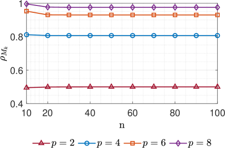
(b) Dirichlet-Neumann system.

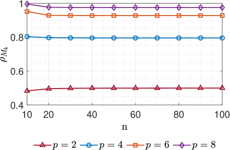
(c) Neumann-Neumann system.

Figure 1: Spectral radius versus number of collocation points for different basis function degree $p$ and different combinations of boundary conditions. Results are the same for both values $k$ can take.

3.2 Linear approximation of the rotational balance equation

As observed in [49], the Newton-Raphson algorithm normally requires only one iteration. This feature suggest that, in an explicit dynamics context where very small time steps are used, the nonlinearity associated with the angular acceleration term in the rotational balance equation is rather weak. On this basis, we explore the appealing possibility to gain a significant advantage in terms of accuracy paying a negligible cost in terms of accuracy. Namely, our assumption is to use directly a linearized form of the rotational balance equation to completely bypass the iterative solution scheme. This is done by substituting one of the two ${\boldsymbol{\alpha}}_{i}^{n}$ appearing in the left hand side of Eq. (25) with ${\boldsymbol{\alpha}}_{i}^{(n-1)}$. Therefore, Eq. (25) becomes linear in ${\boldsymbol{\alpha}}_{i}^{n}$ and reads as follows

$$\left[{\boldsymbol{j}}_{i}^{n}+{\widetilde{\left(\frac{h}{2}\,{\boldsymbol{\omega}}^{(n-1)}_{p,i}+\frac{h^{2}}{4}\,{\boldsymbol{\alpha}}_{i}^{(n-1)}\right)}}{\boldsymbol{j}}_{i}^{n}\right]{\boldsymbol{\alpha}}_{i}^{n}={\boldsymbol{\chi}}^{n}_{i}-[{\boldsymbol{\omega}}^{(n-1)}_{p,i}+\frac{h}{2}\,{\boldsymbol{\alpha}}_{i}^{(n-1)}]\times{\boldsymbol{(}}j_{i}^{n}{\boldsymbol{\omega}}^{(n-1)}_{p,i})\,,$$ (49)

Eq. (49) is then discretized in space and rearranged following the same procedure presented in Section 3.1.

To recap, the proposed solution procedure is based on three modifications of the existing formulation: i) the decoupling of the Neumann boundary conditions; ii) the rearrangement of the system of equations to obtain a banded mass matrix, ${\boldsymbol{M}}$, containing only basis functions and their derivatives evaluated at the collocation points (see Eq. (49)); iii) the use of a linearized form of the rotational balance equation to avoid the iterative scheme. We remark that, with these modifications, it is possible to subdivide the $6\rm{n}\times 6\rm{n}$ system of equations into two $3\rm{n}\times 3\rm{n}$ subsystems, on which the predictor–multicorrector approach can be applied separately.

4 Numerical results and discussion

In this section, we present the results of the proposed fully explicit IGA-C solution procedure, referred to as LU L (LUmped Linear), and compare it with the one in [50] employing a consistent mass matrix and solving the original nonlinear system. We refer to the latter consistent nonlinear form as CN NL. Moreover, to assess our assumption on the linear form of the rotational equation, we provide the results of the predictor–multicorrector approach applied to the nonlinear system of equations (Eqs. (39) and (40)). We refer to this formulation as LU NL (LUmped NonLinear). With this additional comparison, we demonstrate that LU L does not introduce any significant loss of accuracy. Note that, as for CN NL, LU NL still requires the Newton-Raphson scheme with the predictor–multicorrector algorithm applied at each iteration.

Four test cases are studied. Firstly, a cantilever beam under a constant tip vertical load is analyzed. Then, we study a swinging flexible pendulum oscillating under self-weight and a three-dimensional flying beam subjected to tip forces and couples. The last numerical test concerns a spinning beam in a gravitational field undergoing rigid-body motions. The study is completed with a comparative analysis of the computational costs.

4.1 Cantilever beam

This problem consist of a straight, $\SI{1}{m}$-long cantilever beam with a square cross section of side length $\SI{0.01}{m}$ [59]. The beam lies along the $x_{2}$-axis and deforms in the $(x_{2},x_{3})$ plane. It is is clamped at one end and loaded at its free end with a concentrated constant force, along $x_{3}$, $F_{3}=\SI{-100}{N}$ (see Figure 2).

\begin{overpic}[width=346.89731pt]{cantilever_long.jpg} \put(925.0,200.0){$F_{3}$} \end{overpic}

Figure 2: Cantilever beam under impulsive load: geometry and applied forces.

The material properties are: density $\rho=\SI{7800}{kg/m^{3}}$, Young’s modulus $E=\SI{210E9}{N/m^{2}}$, and Poisson’s ratio $\nu=0.2$. Figure 3 shows the time history of the tip displacement. The black solid line refers to the consistent nonlinear formulation (CN NL) [49], whereas the blue dashed line to the lumped nonlinear (LU NL) formulation, and the orange dashed line to the lumped linear one (LU L). Overall, a very good agreement is observed. At the beginning of the simulation the three formulations are almost identical. As time goes (see, e.g., the peak at ca 0.465s), a slight difference is observed in the LU L.

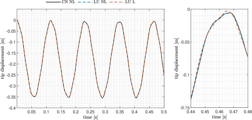
Figure 3: Tip displacement of a cantilever beam subjected to a tip force $F_{3}=\SI{-100}{N}$. $p=4$, $\rm n=20$, $h=\SI{1E-6}{s}$: results for the entire simulation time (left) and close-up for $t\in[\SI{0.44}{},\SI{0.48}{}]\,\SI{}{s}$ (right).

To assess the spatial accuracy of the proposed methods, we perform a convergence study of the $L_{2}$-norm of the error, $err_{L_{2}}=||{\boldsymbol{u}}^{h}-{\boldsymbol{u}}^{r}||_{L_{2}}/||{\boldsymbol{u}}^{r}||_{L_{2}}$, where ${\boldsymbol{u}}^{h}$ and ${\boldsymbol{u}}^{r}$ are the approximated and reference displacements, respectively, evaluated at $t=\SI{0.001}{s}$ and computed over a fixed grid of equally spaced points. For each approach, the reference solution is computed with $p=6$, $\rm n=80$ and $h=\SI{1e-7}{s}$. In order to minimize the effects of the temporal error, the time step size is reduced when $\rm n$ and $p$ are increased [50]. The convergence curves are shown in Figure 4. The CN NL case is presented in Figure 4a, whereas LU NL and LU L in Figure 4b and  4c, respectively. No differences are observed in the rates among the three approaches, demonstrating the capability of the proposed fully explicit method, LU L, to keep the same IGA-C high-order space accuracy of the reference formulation CN NL. Concerning $p=2$, it shows a slower convergence as documented also in [49, 50].

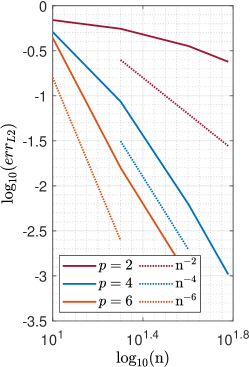
(a) CN NL.

(b) LU NL.

(c) LU L.

Figure 4: Cantilever beam under tip load: convergence plots for $p=2,4,6$ vs. number of collocation points of the three solution procedures.

4.2 Swinging flexible pendulum

This test concerns a pendulum swinging under the action of its self-weight (see Figure 5). The beam presents the same initial geometry of the cantilever case (see Section 4.1), but it is hinged at one end and has a circular cross-section of diameter $\SI{0.01}{m}$ [60, 61, 62, 63]. The material properties, the same as in [50], are $E=\SI{5E6}{N/m^{2}}$, $\nu=0.5$, and $\rho=\SI{1100}{kg/m^{3}}$.

\begin{overpic}[width=346.89731pt]{pendulum.jpg} \put(1000.0,250.0){$q_{3}$} \end{overpic}

Figure 5: Swinging flexible pendulum subjected to a distributed vertical load.

The spatial discretization relies on basis functions of degree $p=4$ and $\rm n=30$ collocation points. The simulation lasts $\SI{1}{s}$ with a time step span $h=\SI{1e-5}{s}$.

Figure 6 shows some snapshots of the swinging beam. The time history of the tip displacement is shown in Figure 7. An excellent agreement is observed for all cases.

Figure 6: Snapshots of a swinging flexible pendulum from time $0$ to $\SI{1}{s}$ with increments of $\SI{0.1}{s}$. $p=4$, $\rm n=30$, $h=\SI{1E-5}{s}$.

Figure 7: Swinging flexible pendulum results for $p=4$, $\rm n=30$, $h=\SI{1E-5}{s}$: tip vertical displacement time history (left) and close up for $t\in[\SI{0.5001}{},\SI{0.5005}{}]\,\SI{}{s}$ (right).

To verify the high order spatial accuracy of the proposed method, convergence plots are shown in Figure 8. The $L_{2}$-norm of the error, $err_{L_{2}}$, is computed on the displacements evaluated at $t=\SI{0.1}{s}$. The reference solution is obtained with $p=6$, $\rm{n}=80$ and $h=\SI{2.5e-6}{s}$. The rates of convergence are studied for $p=2,4,6$ with $\rm{n}=10,20,40,60$ and time step sizes equal to $\SI{5e-5}{}$, $\SI{2.5e-5}{}$, $\SI{1.25e-5}{}$ and $\SI{5e-6}{}$, respectively. Compared to the reference case, CN NL, excellent rates are achieved also with LU NL and LU L, proving again the

(a) CN NL.

(b) LU NL.

(c) LU L.

Figure 8: Swinging flexible pendulum: convergence plots for $p=2,4,6$ vs. number of collocation points of the three solution procedures.

4.3 Three-dimensional free flying beam

With this numerical example, we test the capabilities of our proposed fully explicit formulation to address the well-known problem of the free flying beam undergoing very large and complex three-dimensional motions and rotations [56, 64, 65, 66, 49, 50]. The same material properties of [56] are used: ${\mathbb{C}}_{N}=\text{diag}(10000,10000,10000)\SI{}{N}$, ${\mathbb{C}}_{M}=\text{diag}(500,500,500)\SI{}{Nm^{2}}$, ${\boldsymbol{J}}=\text{diag}(10,10,10)\SI{}{kgm^{2}}$, and $\mu=\SI{1}{kg/m}$.

Figure 9 shows the initial shape of the beam and the load time histories applied to one of the free ends of the beam. The beam axis is discretized with $p=6$ B-Splines and $\rm n=60$ collocation points. The total simulation time is $T=\SI{5}{s}$ with a time step size of $h=\SI{5e-6}{s}$.

(a) Initial configuration and loads.

(b) Load time histories

​

Figure 9: Flying flexible beam: initial configuration and loads [50].

Snapshots of the deformed configurations obtained with the three different formulations, CN NL, LU NL, and LU L, are plotted in Figure 10. No distinguishable differences are observed among the formulations.

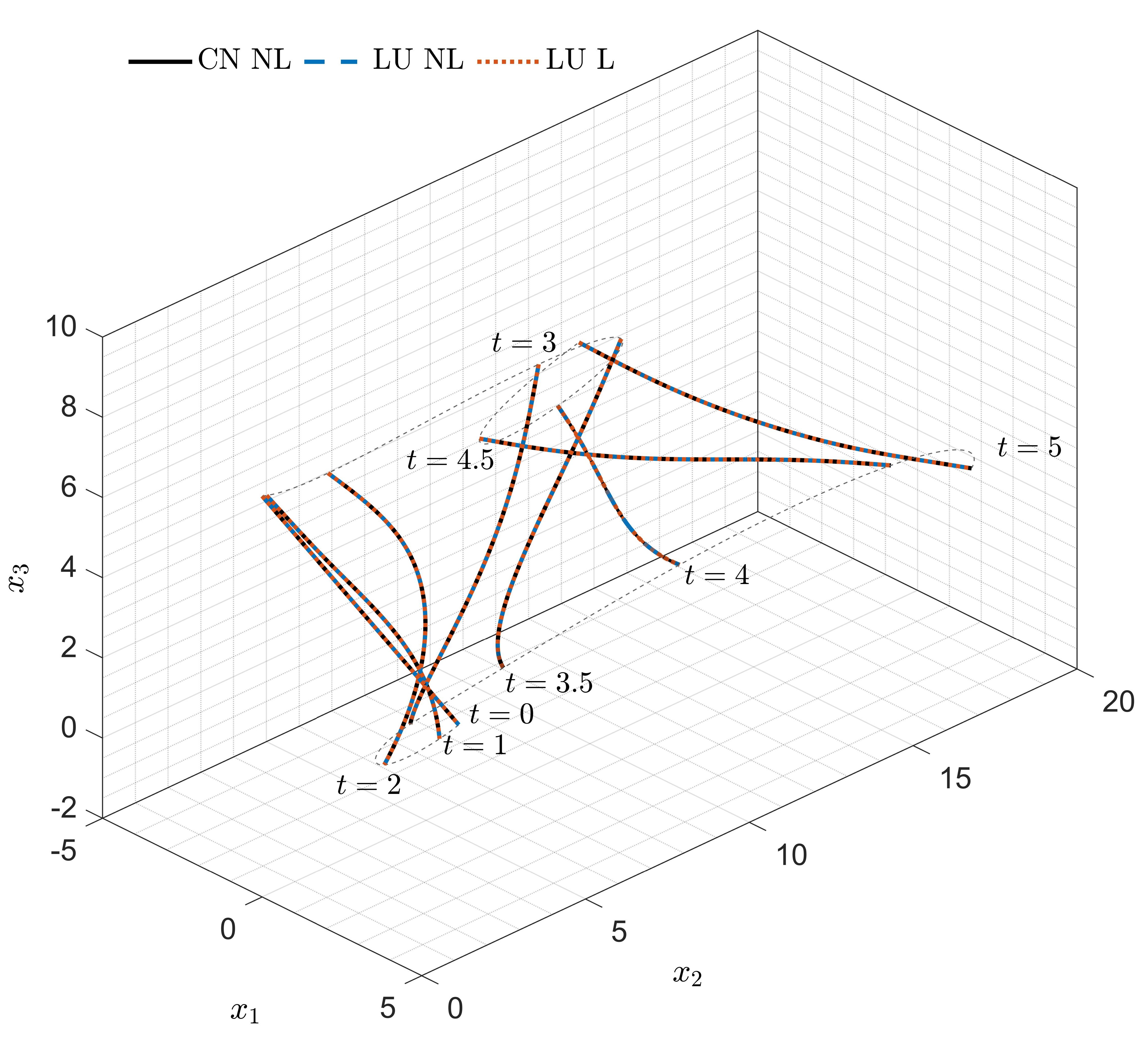
Figure 10: Flying flexible beam: snapshots of the deformed configurations obtained with $p=6$, $\rm n=60$ and $h=\SI{5e-6}{s}$.

The spatial convergence rates of the $L_{2}$-norm of the error $err_{L_{2}}=||{\boldsymbol{c}}^{h}-{\boldsymbol{c}}^{r}||_{L_{2}}/||{\boldsymbol{c}}^{r}||_{L_{2}}$ computed at $t=\SI{0.5}{s}$ are shown in Figure 11. ${\boldsymbol{c}}^{h}$ and ${\boldsymbol{c}}^{r}$ are the approximate and reference position vectors of the beam centroid, respectively, The reference solution is obtained with $p=6$ and $\rm{n}=150$, and $h=\SI{5e-6}{s}$. The dominance of the temporal error over the spatial one is clearly noticeable as the convergence rates do not go beyond the fourth order. However, we remark that the rates of both LU NL and LU L are identical to the reference formulation CN NL (Figure 11a). This clearly indicates that the sub-optimal rates for $p=6$ are not ascribable neither to the mass lumping nor to the the linearization of the rotational equations, but only to the low (second-) order accuracy of the time integrator.

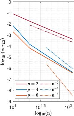
(a) CN NL.

(b) LU NL.

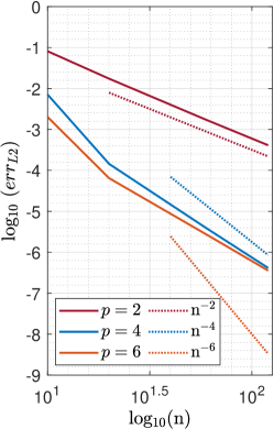
(c) LU L.

Figure 11: Free flying beam: convergence plots for $p=2,4,6$ vs. number of collocation points of the three solution procedures.

4.4 Spinning beam in a gravitational field

In this last numerical example we consider a spinning beam in a gravitational field. This test is carried out to further test the capabilities of the proposed method to address large and mainly rigid-body rotations, since the elastic deformations are very small. The same beam considered in Section 4.1, but with a different square cross-section of side length $\SI{0.0175}{m}$, is hinged at one of its end and loaded by its self-weight, $q_{3}$ (see Figure 12). Additionally, we prescribe an initial angular velocity to each beam point, ${\boldsymbol{\omega}}^{0}=[0,0,\omega^{0}_{3}]^{\mathsf{{\scriptscriptstyle{\!}}T}}$. We select three different values for $\omega^{0}_{3}$: i) $\omega^{0}_{3}=0.2\pi$, reproducing a very slow spinning beam dominated by the gravitational load and leading to large three-dimensional motions; ii) $\omega^{0}_{3}=2\pi$, where we have a combination of fast rotations and out-of-plane deflections; iii) $\omega^{0}_{3}=20\pi$, where the angular velocity is sufficiently high to keep the rigid-body motion almost entirely in the plane $(x_{1},x_{2})$.

\begin{overpic}[width=260.17464pt]{spinning_beam_conf.jpg} \put(-30.0,575.0){$q_{3}$} \put(975.0,270.0){${\boldsymbol{\omega}}^{0}$} \end{overpic}

Figure 12: Spinning beam under gravitational load.

Snapshots of the beam motion and tip displacement time histories are reported in Figures 13, 14 and 15 for $\omega^{0}_{3}=0.2\pi,\,2\pi$ and $20\pi$, respectively. Compared to the reference formulation CN NL, excellent results are obtained by both LU NL and LU L lumping schemes.

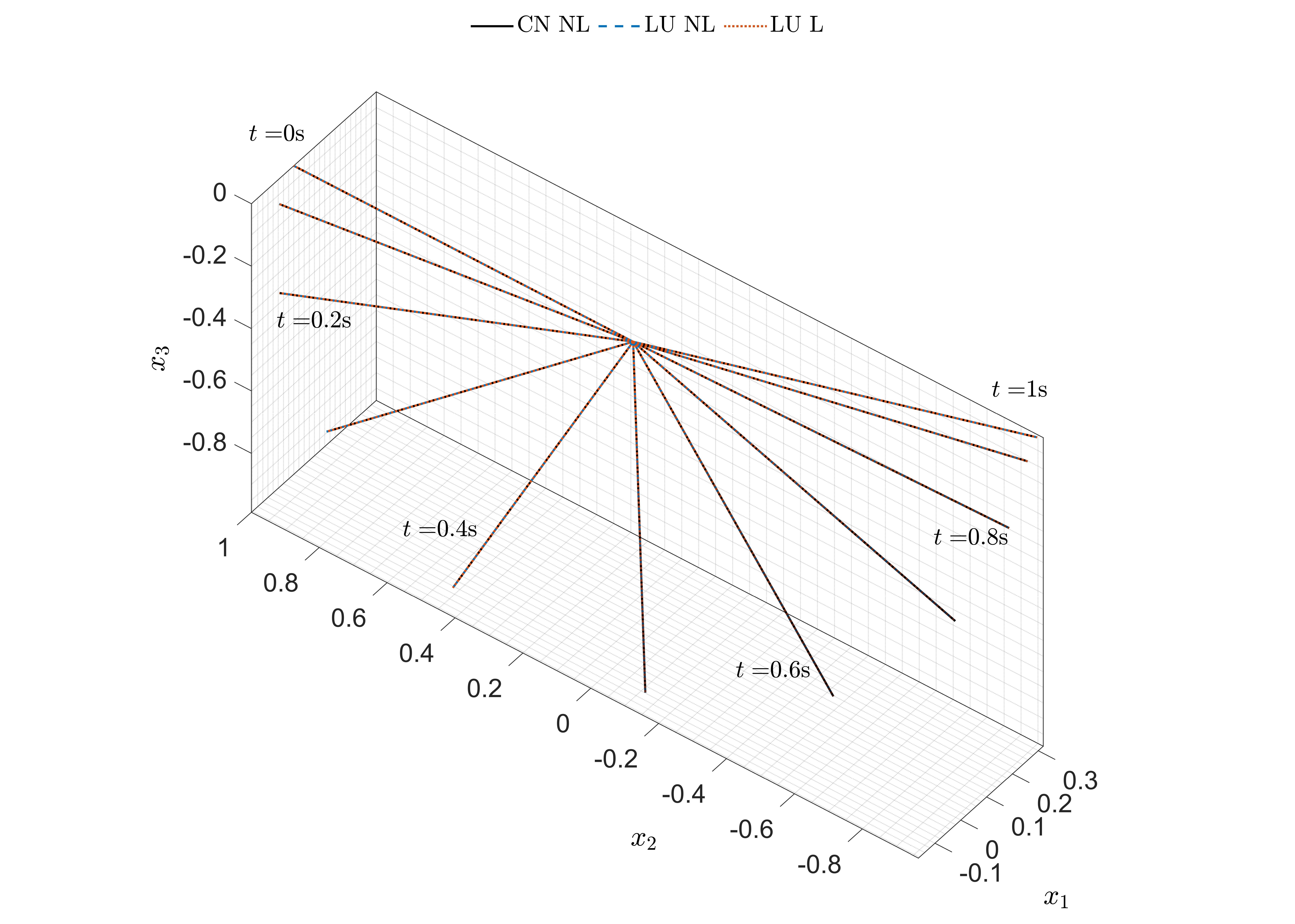
(a) Snapshots of the beam motion obtained with $p=4$, $\rm{n}=20$ and $h=\SI{1e-6}{s}$.

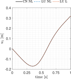
(b) Tip displacement time history along the $x_{1}$-axis.

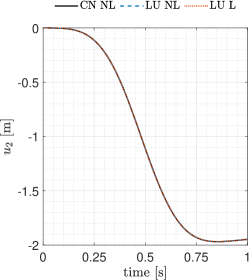
(c) Tip displacement time history along the $x_{2}$-axis.

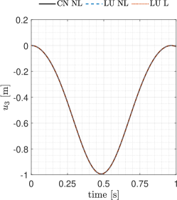
(d) Tip displacement time history along the $x_{3}$-axis.

Figure 13: Spinning beam in a gravitational field: results with initial angular velocity, $\omega^{0}_{3}=0.2\pi$.

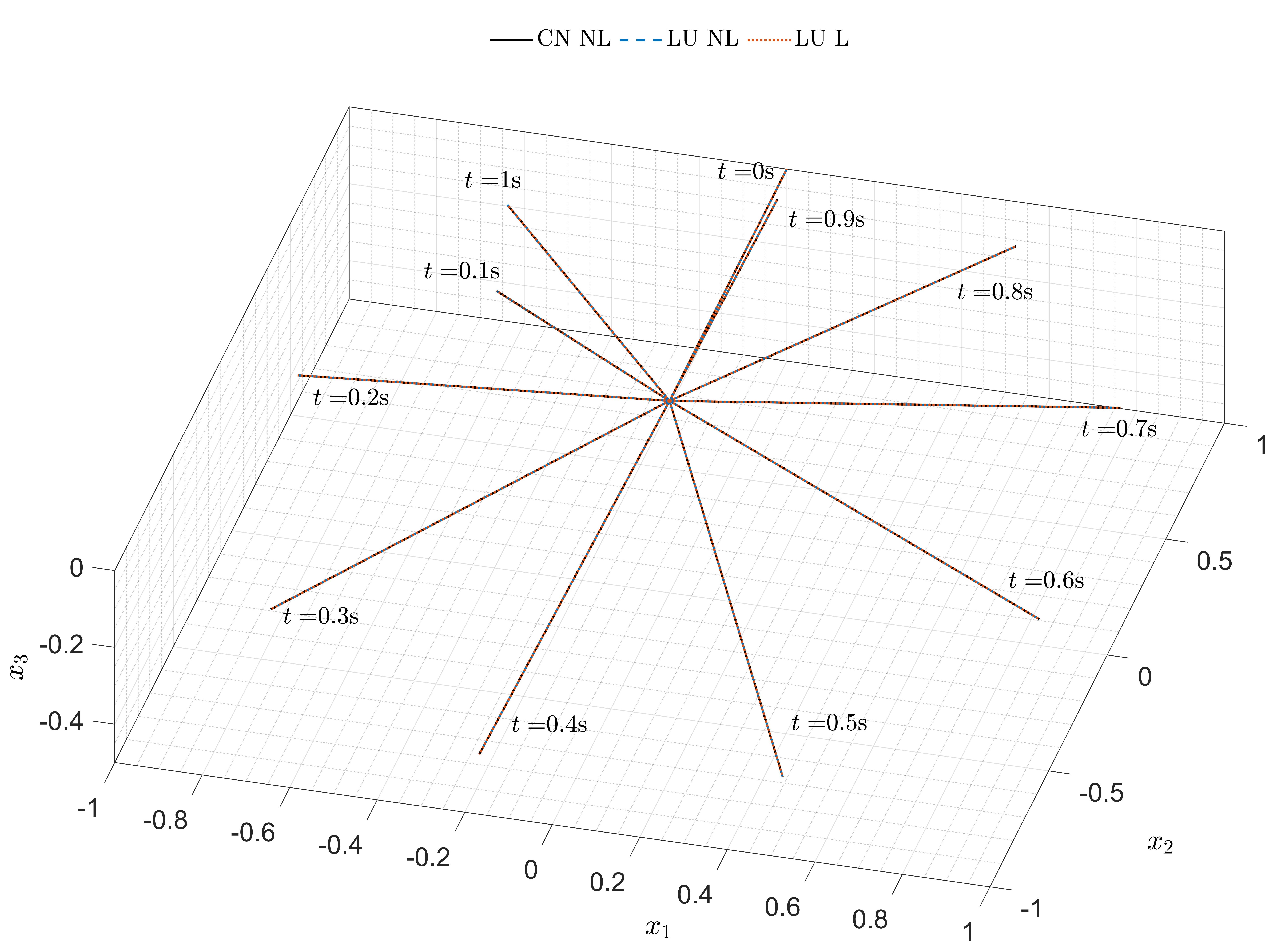
(a) Snapshots of the beam motion obtained with $p=4$, $\rm{n}=20$ and $h=\SI{1e-6}{s}$.

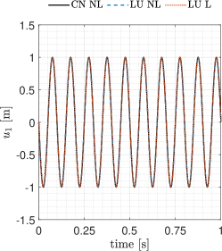
(b) Tip displacement time history along the $x_{1}$-axis.

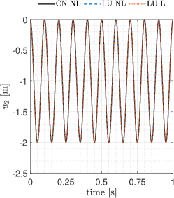
(c) Tip displacement time history along the $x_{2}$-axis.

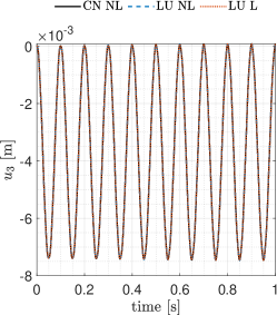
(d) Tip displacement time history along the $x_{3}$-axis.

Figure 14: Spinning beam in a gravitational field: results with initial angular velocity $\omega^{0}_{3}=2\pi$.

(a) Snapshots of the beam motion obtained with $p=4$, $\rm{n}=20$ and $h=\SI{1e-6}{s}$.

(b) Tip displacement time history along the $x_{1}$-axis.

(c) Tip displacement time history along the $x_{2}$-axis.

(d) Tip displacement time history along the $x_{3}$-axis.

Figure 15: Spinning beam in a gravitational field: results with initial angular velocity, $\omega^{0}_{3}=20\pi$.

4.5 Considerations on the efficiency of the formulations

In this section, we provide a comparison in terms of computational time among the three formulations: lumped linear, LU L, lumped nonlinear, LU NL, and the reference one, i.e., consistent nonlinear CN NL.

For each of them, numerical simulations are performed for different values of $p$ and $\rm{n}$, keeping the time size $h$ fixed to the value adopted for the respective overkill solutions. The total time is set to $500h$. The efficiency is estimated calculating the average CPU time required for a single time step, $h_{\rm{CPU}}$. Since the scope of this study is to provide quantitative comparisons, rather than to rigorously estimate the computational performances of each formulation, results are plotted in terms of normalized CPU time steps, $h^{{n}}_{\rm{CPU}}=h_{\rm{CPU}}/h^{r}_{\rm{CPU}}$. For a given degree $p$, the reference value, $h^{r}_{\rm{CPU}}$, is taken as the average CPU time per time step obtained with $\rm{n}=10$ collocation points using the reference CN NL formulation.

Results are presented for the cantilever beam in Figure 16, for the swinging pendulum in Figure 17, for the flying beam in Figure 18, and for the fast spinning beam ($\omega^{0}_{3}=20\pi$) in Figure 19 (similar curves are observed for $\omega^{0}_{3}=0.2\pi,\,2\pi$, therefore associated plots are not reported). Solid lines refer to the CN NL case, whereas dashed and dashed dotted lines to LU NL and LU L formulations, respectively. The same colors adopted in the spatial convergence plots (see Figures 4, 8, and 11) are here employed for $p=2$ (dark red lines in Figures 16a–18a), $p=4$ (blue lines in Figures 16b–18b), $p=6$ (orange lines in Figures 16c–18c) curves.

The LU L formulation exhibits always the lowest $h^{{n}}_{\rm{CPU}}$. In particular, it is noted that the most significant CPU time reduction occurs for large values of $\rm{n}$, meaning that the proposed method has the potential to dramatically increase the efficiency in simulations of complex beams systems with a high number of degrees of freedom, still preserving the high-order accuracy typical of IGA-C. Moreover, except for the clamped case with $p=4,6$ (see Figure 16) and for the spinning beam with $p=6$ (see Figure 19), the LU NL formulation is faster than the CN NL one, even with a low number of collocation points. As expected, as $p$ increases, the efficiency gain tends to reduce due to a larger spectral radius (see Figures 1) which requires more corrector passes.

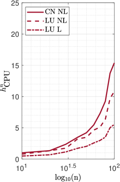
(a) $p=2$.

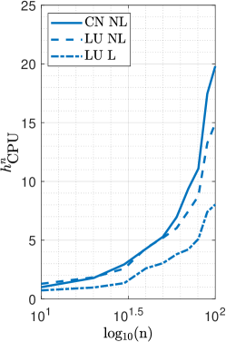
(b) $p=4$.

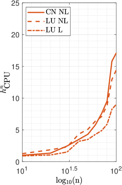
(c) $p=6$.

Figure 16: Normalized CPU time per time step vs. number of collocation points for the cantilever beam.

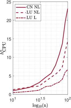
(a) $p=2$.

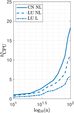
(b) $p=4$.

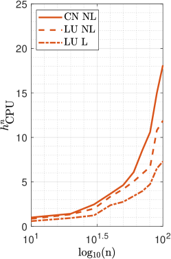
(c) $p=6$.

Figure 17: Normalized CPU time per time step vs. number of collocation points for the swinging flexible pendulum.

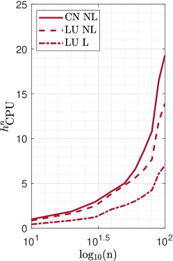
(a) $p=2$.

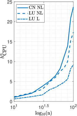
(b) $p=4$.

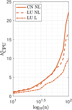
(c) $p=6$.

Figure 18: Normalized CPU time per time step vs. number of collocation points for the free flying beam.

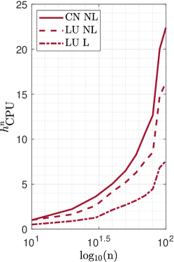
(a) $p=2$.

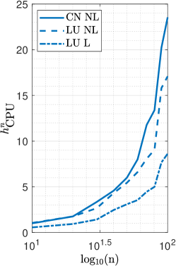
(b) $p=4$.

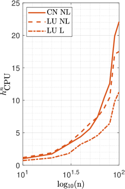
(c) $p=6$.

Figure 19: Normalized CPU time per time step vs. number of collocation points for the spinning beam with $\omega^{0}_{3}=20\pi$.

5 Conclusions

In this paper, we proposed a fully explicit dynamic IGA-C formulation for geometrically exact beams. Starting from an existing formulation, which is explicit only in the strict sense of the time integration algorithm, we made the method fully explicit adapting an existing predictor–multicorrector method, originally proposed for standard linear elastodynamics, to the case of the finite rotational dynamics of geometrically exact beams.

The procedure relies on decoupling the Neumann boundary conditions and on a rearrangement and rescaling of the mass matrix. Moreover, we pursued additional efficiency removing the angular velocity-dependent nonlinear term in the rotational balance equation, bypassing the need for a time-consuming iterative scheme. The performance of the method is tested with three numerical applications involving both Dirichlet-Neumann and Neumann-Neumann boundary conditions.

We demonstrated that the proposed method preserves the same high-order spatial accuracy as the “exact” case where a consistent mass matrix and the full nonlinear rotational balance equation are used. We also quantified the gain in terms of computational cost and demonstrated that the proposed method significantly decreases the computational time without losing accuracy. This gain increases with the number of collocation points, indicating that the proposed lumping scheme has the potential to manage complex dynamic problems with many degrees of freedom which would be not affordable with methods using the consistent mass matrix. In some cases, we found that the temporal error dominates the spatial one, regardless of the mass matrix used. Therefore, future works will be devoted to the development of $\operatorname{{{\rm SO(3)}}}3$-consistent beam dynamic formulations with higher-order accuracy for both space and time. Given the raising interest in the dynamics of multi-body and complex-shaped systems, such as mechanical meta-materials, future developments will also include multi-patch structures.

References

- [1] P. Otto, L. De Lorenzis, J. F. Unger, Explicit dynamics in impact simulation using a NURBS contact interface, International Journal for Numerical Methods in Engineering 121 (6) (2020) 1248–1267. doi:10.1002/nme.6264.
- [2] W. Sun, T. Zhu, P. Chen, G. Lin, Dynamic implosion of submerged cylindrical shell under the combined hydrostatic and shock loading, Thin-Walled Structures 170 (July 2021) (2022) 108574. doi:10.1016/j.tws.2021.108574.
- [3] S. R. Wu, Lumped mass matrix in explicit finite element method for transient dynamics of elasticity, Computer Methods in Applied Mechanics and Engineering 195 (44-47) (2006) 5983–5994. doi:10.1016/j.cma.2005.10.008.
- [4] T. Elguedj, A. Gravouil, H. Maigre, An explicit dynamics extended finite element method. Part 1: Mass lumping for arbitrary enrichment functions, Computer Methods in Applied Mechanics and Engineering 198 (30-32) (2009) 2297–2317. doi:10.1016/j.cma.2009.02.019.
- [5] T. Menouillard, J. Réthoré, S. Moes, A. Combescure, H. Bung, Mass lumping strategies for X-FEM explicit dynamics: Application to crack propagation, International Journal for Numerical Methods in Engineering (February) (2012) 1102–1119. doi:10.1002/nme.
- [6] Y. Yang, H. Zheng, M. V. Sivaselvan, A rigorous and unified mass lumping scheme for higher-order elements, Computer Methods in Applied Mechanics and Engineering 319 (2017) 491–514. doi:10.1016/j.cma.2017.03.011.
- [7] H. Gravenkamp, C. Song, J. Zhang, On mass lumping and explicit dynamics in the scaled boundary finite element method, Computer Methods in Applied Mechanics and Engineering 370 (2020) 113274. doi:10.1016/j.cma.2020.113274.
- [8] Y. Voet, E. Sande, A. Buffa, A mathematical theory for mass lumping and its generalization with applications to isogeometric analysis, Computer Methods in Applied Mechanics and Engineering 410 (2023) 116033. arXiv:2212.03614, doi:10.1016/j.cma.2023.116033.
- [9] J. A. Cottrell, A. Reali, Y. Bazilevs, T. J. Hughes, Isogeometric analysis of structural vibrations, Computer Methods in Applied Mechanics and Engineering 195 (41-43) (2006) 5257–5296. doi:10.1016/j.cma.2005.09.027.
- [10] A. Tkachuk, M. Bischoff, Direct and sparse construction of consistent inverse mass matrices: general variational formulation and application to selective mass scaling, Int. J. Numer. Meth. Engng (October) (2015) 1102–1119. doi:10.1002/nme.
- [11] A. K. Schaeuble, A. Tkachuk, M. Bischoff, Variationally consistent inertia templates for B-spline- and NURBS-based FEM: Inertia scaling and customization, Computer Methods in Applied Mechanics and Engineering 326 (2017) 596–621. doi:10.1016/j.cma.2017.08.035.
- [12] S. Duczek, H. Gravenkamp, Mass lumping techniques in the spectral element method: On the equivalence of the row-sum, nodal quadrature, and diagonal scaling methods, Computer Methods in Applied Mechanics and Engineering 353 (2019) 516–569. doi:10.1016/j.cma.2019.05.016.
- [13] T. Hughes, J. Cottrell, Y. Bazilevs, Isogeometric analysis: CAD, finite elements, NURBS, exact geometry and mesh refinement, Computer Methods in Applied Mechanics and Engineering 194 (39-41) (2005) 4135–4195.
- [14] L. Piegl, W. Tiller, The NURBS Book, Springer, 1997.
- [15] J. A. Cottrell, T. J. R. Hughes, Y. Bazilevs, Isogeometric analysis: toward integration of CAD and FEA, JohnWiley & Sons, Ltd Registered, 2009.
- [16] C. Anitescu, C. Nguyen, T. Rabczuk, X. Zhuang, Isogeometric analysis for explicit elastodynamics using a dual-basis diagonal mass formulation, Computer Methods in Applied Mechanics and Engineering 346 (2019) 574–591. doi:10.1016/j.cma.2018.12.002.
- [17] X. Li, D. Wang, On the significance of basis interpolation for accurate lumped mass isogeometric formulation, Computer Methods in Applied Mechanics and Engineering 400 (2022) 115533. doi:10.1016/j.cma.2022.115533.
- [18] T. H. Nguyen, R. R. Hiemstra, S. Eisenträger, D. Schillinger, Towards higher-order accurate mass lumping in explicit isogeometric analysis for structural dynamics, Computer Methods in Applied Mechanics and Engineering (xxxx) (2023) 116233. arXiv:2305.12916, doi:10.1016/j.cma.2023.116233.
- [19] F. Auricchio, L. B. Da Veiga, T. J. R. Hughes, a. Reali, G. Sangalli, Isogeometric Collocation Methods, Mathematical Models and Methods in Applied Sciences 20 (11) (2010) 2075–2107.
- [20] F. Auricchio, L. Beirão da Veiga, T. J. R. Hughes, a. Reali, G. Sangalli, Isogeometric collocation for elastostatics and explicit dynamics, Computer Methods in Applied Mechanics and Engineering 249-252 (2012) 2–14.
- [21] D. Schillinger, J. Evans, A. Reali, M. Scott, T. J. Hughes, Isogeometric collocation: Cost comparison with Galerkin methods and extension to adaptive hierarchical NURBS discretizations, Computer Methods in Applied Mechanics and Engineering 267 (2013) 170–232.
- [22] C. Adam, T. Hughes, S. Bouabdallah, M. Zarroug, H. Maitournam, Selective and reduced numerical integrations for NURBS-based isogeometric analysis, Computer Methods in Applied Mechanics and Engineering 284 (2015) 732–761.
- [23] F. Fahrendorf, L. De Lorenzis, H. Gomez, Reduced integration at superconvergent points in isogeometric analysis, Computer Methods in Applied Mechanics and Engineering 328 (2018) 390–410.
- [24] G. Sangalli, M. Tani, Matrix-free weighted quadrature for a computationally efficient isogeometric k-method, Computer Methods in Applied Mechanics and Engineering 338 (2018) 117–133.
- [25] R. Kruse, N. Nguyen-Thanh, L. De Lorenzis, T. Hughes, Isogeometric collocation for large deformation elasticity and frictional contact problems, Computer Methods in Applied Mechanics and Engineering 296 (2015) 73–112.
- [26] F. Fahrendorf, S. Morganti, A. Reali, T. J. Hughes, L. D. Lorenzis, Mixed stress-displacement isogeometric collocation for nearly incompressible elasticity and elastoplasticity, Computer Methods in Applied Mechanics and Engineering 369 (2020) 113112. doi:10.1016/j.cma.2020.113112.
- [27] H. Gomez, A. Reali, G. Sangalli, Accurate, efficient, and (iso)geometrically flexible collocation methods for phase-field models., Journal for Computational Physics 262 (2014) 153–171.
- [28] D. Schillinger, M. J. Borden, H. K. Stolarski, Isogeometric collocation for phase-field fracture models, Computer Methods in Applied Mechanics and Engineering 284 (2015) 583–610. doi:10.1016/J.CMA.2014.09.032.
- [29] P. Fedeli, A. Frangi, F. Auricchio, A. Reali, Phase-field modeling for polarization evolution in ferroelectric materials via an isogeometric collocation method, Computer Methods in Applied Mechanics and Engineering 351 (2019) 789–807. doi:10.1016/j.cma.2019.04.001.
- [30] L. De Lorenzis, J. Evans, T. Hughes, A. Reali, Isogeometric collocation: Neumann boundary conditions and contact, Computer Methods in Applied Mechanics and Engineering 284 (2015) 21–54.
- [31] O. Weeger, B. Narayanan, L. De Lorenzis, J. Kiendl, M. L. Dunn, An isogeometric collocation method for frictionless contact of Cosserat rods, Computer Methods in Applied Mechanics and Engineering 321 (2017) 361–382.
- [32] L. Beirão da Veiga, C. Lovadina, a. Reali, Avoiding shear locking for the Timoshenko beam problem via isogeometric collocation methods, Computer Methods in Applied Mechanics and Engineering 241-244 (2012) 38–51.
- [33] F. Auricchio, L. Beirão da Veiga, J. Kiendl, C. Lovadina, a. Reali, Locking-free isogeometric collocation methods for spatial Timoshenko rods, Computer Methods in Applied Mechanics and Engineering 263 (2013) 113–126.
- [34] J. Kiendl, F. Auricchio, T. Hughes, A. Reali, Single-variable formulations and isogeometric discretizations for shear deformable beams, Computer Methods in Applied Mechanics and Engineering 284 (2015) 988–1004.
- [35] J. Kiendl, F. Auricchio, A. Reali, A displacement-free formulation for the Timoshenko beam problem and a corresponding isogeometric collocation approach, Meccanica (2017) 1–11.
- [36] G. Balduzzi, S. Morganti, F. Auricchio, Non-prismatic Timoshenko-like beam model: Numerical solution via isogeometric collocation, Computers & Mathematics with Applications 74 (2017) 1531–1541. doi:10.1016/J.CAMWA.2017.04.025.
- [37] A. Reali, H. Gomez, An isogeometric collocation approach for Bernoulli-Euler beams and Kirchhoff plates, Computer Methods in Applied Mechanics and Engineering 284 (2015) 623–636.
- [38] E. Marino, S. F. Hosseini, A. Hashemian, A. Reali, Effects of parameterization and knot placement techniques on primal and mixed isogeometric collocation formulations of spatial shear-deformable beams with varying curvature and torsion, Computers and Mathematics with Applications 80 (2020) 2563–2585. doi:10.1016/j.camwa.2020.06.006.
- [39] D. Ignesti, G. Ferri, F. Auricchio, A. Reali, E. Marino, An improved isogeometric collocation formulation for spatial multi-patch shear-deformable beams with arbitrary initial curvature, Computer Methods in Applied Mechanics and Engineering 403 (2023) 115722. doi:10.1016/j.cma.2022.115722.
- [40] F. Maurin, F. Greco, S. Dedoncker, W. Desmet, Isogeometric analysis for nonlinear planar kirchhoff rods: Weighted residual formulation and collocation of the strong form, Computer Methods in Applied Mechanics and Engineering (2018). doi:10.1016/j.cma.2018.05.025.
- [41] J. Kiendl, F. Auricchio, L. Beirão da Veiga, C. Lovadina, A. Reali, Isogeometric collocation methods for the Reissner-Mindlin plate problem, Computer Methods in Applied Mechanics and Engineering 284 (2015) 489–507.
- [42] J. Kiendl, E. Marino, L. De Lorenzis, Isogeometric collocation for the Reissner-Mindlin shell problem, Computer Methods in Applied Mechanics and Engineering 325 (2017) 645–665.
- [43] F. Maurin, F. Greco, L. Coox, D. Vandepitte, W. Desmet, Isogeometric collocation for Kirchhoff-Love plates and shells, Computer Methods in Applied Mechanics and Engineering 329 (2018) 396–420.
- [44] M. Torre, S. Morganti, A. Nitti, M. D. de Tullio, F. S. Pasqualini, A. Reali, Isogeometric mixed collocation of nearly-incompressible electromechanics in finite deformations for cardiac muscle simulations, Computer Methods in Applied Mechanics and Engineering 411 (2023) 116055. doi:10.1016/J.CMA.2023.116055.
- [45] E. Marino, Isogeometric collocation for three-dimensional geometrically exact shear-deformable beams, Computer Methods in Applied Mechanics and Engineering 307 (2016) 383–410.
- [46] E. Marino, Locking-free isogeometric collocation formulation for three-dimensional geometrically exact shear-deformable beams with arbitrary initial curvature, Computer Methods in Applied Mechanics and Engineering 324 (2017) 546–572.
- [47] G. Ferri, D. Ignesti, E. Marino, An efficient displacement-based isogeometric formulation for geometrically exact viscoelastic beams, Computer Methods in Applied Mechanics and Engineering 417 (2023) 116413. arXiv:2307.10106, doi:10.1016/j.cma.2023.116413.
- [48] O. Weeger, S.-K. Yeung, M. L. Dunn, Isogeometric collocation methods for Cosserat rods and rod structures, Computer Methods in Applied Mechanics and Engineering 316 (2017) 100–122.
- [49] E. Marino, J. Kiendl, L. De Lorenzis, Explicit isogeometric collocation for the dynamics of three-dimensional beams undergoing finite motions, Computer Methods in Applied Mechanics and Engineering 343 (2019) 530–549. doi:10.1016/j.cma.2018.09.005.
- [50] E. Marino, J. Kiendl, L. D. Lorenzis, Isogeometric collocation for implicit dynamics of three-dimensional beams undergoing finite motions, Computer Methods in Applied Mechanics and Engineering 356 (2019) 548–570. doi:10.1016/J.CMA.2019.07.013.
- [51] J. A. Evans, R. R. Hiemstra, T. J. R. Hughes, A. Reali, Explicit higher-order accurate isogeometric collocation methods for structural dynamics, Computer Methods in Applied Mechanics and Engineering (2018) doi:10.1016/j.cma.2018.04.008.
- [52] G. Ferri, E. Marino, An isogemetric analysis formulation for the dynamics of geometrically exact viscoelastic beams and beam systems with arbitrarily curved initial geometry, Computer Methods in Applied Mechanics and Engineering 431 (2024) 117261. doi:https://doi.org/10.1016/j.cma.2024.117261.
- [53] P. Krysl, L. Endres, Explicit Newmark/Verlet algorithm for time integration of the rotational dynamics of rigid bodies, International Journal for Numerical Methods in Engineering 62 (15) (2005) 2154–2177.
- [54] J. C. Simo, A finite strain beam formulation. The three-dimensional dynamic problem. Part I, Computer Methods in Applied Mechanics and Engineering 49 (1) (1985) 55–70.
- [55] J. Argyris, An excursion into large rotations, Computer Methods in Applied Mechanics and Engineering 32 (1–3) (1982) 85–155.
- [56] L. Simo, J. C. and Vu-Quoc, On the dynamics in space of rods undergoing large motions — A geometrically exact approach, Computer Methods in Applied Mechanics and Engineering 66 (2) (1988) 125–161.
- [57] J. Mäkinen, Total Lagrangian Reissner’s geometrically exact beam element without singularities, International Journal for Numerical Methods in Engineering 70 (October 2006) (2007) 1009–1048.
- [58] J. Mäkinen, Rotation manifold SO(3) and its tangential vectors, Computational Mechanics 42 (6) (2008) 907–919.
- [59] A. Gravouil, A. Combescure, Multi-time-step explicit-implicit method for non-linear structural dynamics, International Journal for Numerical Methods in Engineering 50 (1) (2001) 199–225.
- [60] O. Weeger, B. Narayanan, M. L. Dunn, Isogeometric collocation for nonlinear dynamic analysis of Cosserat rods with frictional contact, Nonlinear Dynamics (2017) 1–15.
- [61] H. Lang, J. Linn, M. Arnold, Multi-body dynamics simulation of geometrically exact Cosserat rods, Multibody System Dynamics 25 (3) (2011) 285–312.
- [62] S. Raknes, X. Deng, Y. Bazilevs, D. Benson, K. Mathisen, T. Kvamsdal, Isogeometric rotation-free bending-stabilized cables: Statics, dynamics, bending strips and coupling with shells, Computer Methods in Applied Mechanics and Engineering 263 (2013) 127–143.
- [63] F. Maurin, L. Dedè, A. Spadoni, Isogeometric rotation-free analysis of planar extensible-elastica for static and dynamic applications, Nonlinear Dynamics 81 (1) (2015) 77–96.
- [64] E. Zupan, M. Saje, D. Zupan, Quaternion-based dynamics of geometrically nonlinear spatial beams using the Runge–Kutta method, Finite Elements in Analysis and Design 54 (2012) 48–60.
- [65] K. M. Hsiao, J. Y. Lin, W. Y. Lin, A consistent co-rotational finite element formulation for geometrically nonlinear dynamic analysis of 3-D beams, Computer Methods in Applied Mechanics and Engineering 169 (1-2) (1999) 1–18.
- [66] R. Zhang, H. Zhong, A quadrature element formulation of an energy–momentum conserving algorithm for dynamic analysis of geometrically exact beams, Computers & Structures 165 (2016) 96–106.