TsCA: On the Semantic Consistency Alignment via Conditional Transport for Compositional Zero-Shot Learning

Abstract

Compositional Zero-Shot Learning (CZSL) aims to recognize novel state-object compositions by leveraging the shared knowledge of their primitive components. Despite considerable progress, effectively calibrating the bias between semantically similar multimodal representations, as well as generalizing pre-trained knowledge to novel compositional contexts, remains an enduring challenge. In this paper, our interest is to revisit the conditional transport (CT) theory and its homology to the visual-semantics interaction in CZSL and further, propose a novel Trisets Consistency Alignment framework (dubbed TsCA) that well-addresses these issues. Concretely, we utilize three distinct yet semantically homologous sets, i.e., patches, primitives, and compositions, to construct pairwise CT costs to minimize their semantic discrepancies. To further ensure the consistency transfer within these sets, we implement a cycle-consistency constraint that refines the learning by guaranteeing the feature consistency of the self-mapping during transport flow, regardless of modality. Moreover, we extend the CT plans to an open-world setting, which enables the model to effectively filter out unfeasible pairs, thereby speeding up the inference as well as increasing the accuracy. Extensive experiments are conducted to verify the effectiveness of the proposed method.

Introduction

Identifying new concepts from a set of seen primitives is one of the fundamental challenges for AI systems to imitate the human learning process. Imagine a new cuisine—Spicy Chocolate Cake. Although it may sound like an odd combination, one can still perceive its appearance and taste based on existing knowledge of ‘spiciness’ and ‘Chocolate’. Likewise, compositional zero-shot learning (CZSL)  (Misra, Gupta, and Hebert 2017; Naeem et al. 2021) emerges as a compelling paradigm that seeks to endow machines with similar cognitive abilities, allowing them to understand the composed primitives (i.e., states and objects) during training and generalize to unseen compositions for inference.

Technically, studies on CZSL have revolved around achieving fine-grained alignment across the image and composed state-object text domains (Huynh and Elhamifar 2020). Pioneer methods typically load pre-trained image encoders and word embeddings to extract multi-modal features. Various alignment tricks are then applied to constrain the shared latent space, including concept learning (Xu, Kordjamshidi, and Chai 2021), geometric properties (Li et al. 2020), semantic transformation (Nagarajan and Grauman 2018), and graph embedding (Mancini et al. 2022). Moving beyond these post-processing alignments, a series of prompt-tuning methods have been developed to explore pre-trained vision-language models (VLMs) for the CZSL scenario (Xu et al. 2022; Nayak, Yu, and Bach 2023), achieving state-of-the-art prediction performance. Pre-trained on massive amounts of image-text pairs, VLMs (e.g., CLIP (Radford et al. 2021)) show impressive abilities to match the visual image with its textual label (prompt) in the multimodal space. Those models often employ a multi-path paradigm for fine-grained textual features, e.g., one composition and two primitive branches. One of the core challenges ensues: How to align the image with such multiple textual labels? Recent studies attempt to address it from different fields, such as hierarchical prompt searching (Wang et al. 2023a), decomposed feature fusion (Lu et al. 2023), and multi-step observation (Li et al. 2023a). Although showing attractive results, these methods focus primarily on image-to-composition (or to-primitive) alignments, ignoring intrinsic relationships within the composition and its primitives. This may fail to capture semantic consistency among the image-composition-primitive interactions, leading to suboptimal alignments.

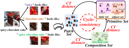
Figure 1: We represent each image as a set of patch embeddings and two sets of textual embeddings and employ semantic consistency conditional transport to align such cross-modal distribution trio.

To address the above issues, this paper proposes the Trisets Consistency Alignment framework (dubbed TsCA), which is built upon a novel Consistency-aware Conditional Transport (CCT) theory derived from the new view of CZSL. As shown in Fig. 1, we represent an image in three directions, i.e., ${\bf P}_{1}$, a distribution over all visual patches; ${\bf P}_{2}$, a distribution over the composition set; and ${\bf P}_{3}$, a distribution over the primitive set. Concretely, ${\bf P}_{1}$ captures the detailed visual features of an image, while ${\bf P}_{2}$ and ${\bf P}_{3}$ denote the global and local textual concepts of the same content. Therefore, the task of CZSL can be viewed as aligning these three discrete distributions as closely as possible. Accordingly, it is indeed key to properly measure the distance between empirical distributions with different supports. Fortunately, conditional transport (CT), well-examined in recent research, offers a bidirectional measurement of the distance from one distribution to another, given the cost matrix. Inheritedly, TsCA extends the minimization of CT to the alignment of our cross-modal distribution trio.

Specifically, TsCA gracefully facilitates the matching of image-composition-primitive triplets by meticulously crafting three pairs of CTs, thereby aligning the rich tapestry of cross-modal and intra-modal semantics. First, $\mathcal{CT}({\bf P}_{1},{\bf P}_{2})$ measures the transport distance between the visual path set ${\bf P}_{1}$ and the composition set ${\bf P}_{2}$. On the one hand, it helps the label be transported to the compositional visuals with higher probabilities, and on the other hand, it regularizes the finetuning for better cross-modal alignments. Next, $\mathcal{CT}({\bf P}_{1},{\bf P}_{3})$ focuses on discovering the corresponding attribute and object patches from the disentangle perspective. Last, unlike the above two, $\mathcal{CT}({\bf P}_{2},{\bf P}_{3})$ aims at intra-modal interactions, which are often overlooked by previous studies. By minimizing the transport distance between the composition and its primitives explicitly, the textual outputs are assumed to present high semantic coherence. E.g., the composition vectors are closer to their primitives in the embedding space. Moreover, the learned transport plan in $\mathcal{CT}({\bf P}_{2},{\bf P}_{3})$ further provides an efficient tool to filter out unfeasible compositions, which benefits the open-world setting.

More importantly, as discussed above, TsCA formulates the CZSL as the alignment of three distributions and seeks to minimize their transport costs. An intuitive solution is to run pairwise transportation and optimize the above three CT costs. Unfortunately, this case could not model the complex relations among these sets. To capture deeper interactions, we extend the naive CT to a well-designed consistency-aware CT (CCT) for the CZSL triplet case. Motivated by the fact that these three distributions describe the same semantics, CCT regularizes the product of three transport plans as a diagonal matrix from two directions (shown in Fig. 1). In other words, the composition label will return to itself after a cycle of transportation, which ensures semantic consistency across sets.

In summary, our contributions are three-fold:

• We formulate the CZSL task as a transport problem and propose Trisets Consistency Alignment model (TsCA), which views an image as three discrete distributions over the patch, composition, and primitive spaces and tries to explore fine-grained alignments between these triplets.

• We develop consistency-aware CT (CCT), considering the semantic consistency across the image-composition-primitive sets, improving the alignment robustness.

• Extensive comparisons and ablations on three benchmarks demonstrate the effectiveness of the proposed TsCA with competitive performance on all settings.

Related Work

Compositional Zero-Shot Learning

CZSL(Mancini et al. 2021) is a specialized case of zero-shot learning (ZSL) (Liu et al. 2023). Given the same set of objects with associated states, it focuses on recognizing unseen state-object compositions by learning from seen compositions. In general, traditional CZSL can be divided into two streams, i.e., compositional classification and simple primitive classification. The former directly predicts compositions by aligning visual features and composed labels in a shared space, or resorting to a graph network for contextuality modeling (Tanwisuth et al. 2023; Saini, Pham, and Shrivastava 2022; Li et al. 2022). Conversely, the latter identifies states and objects independently and constructs the joint compositional probability distribution. They either disregard the contextuality between primitives or impose training-specific correlations that are detrimental to generalization.

Recently, equipped with prompt learning, large-scale VLMs like CLIP are empowered to adapt to CZSL by reducing domain shift and leveraging pre-trained knowledge. Further, researchers attempt to explore merging those two typical paradigms to create an integrated multi-path paradigm. For instance, HPL (Wang et al. 2023a) learns three hierarchical prompts by explicitly fixing the unrelated word tokens in the three embedding spaces at different levels. Troika (Huang et al. 2024) effectively aligns the branch-specific prompt representations and decomposed visual features with a cross-modal traction module. Our TsCA aligns closely with this paradigm, although with a greater emphasis on direct inquiries into semantic alignment within distributions.

Conditional Transport

Recently, CT has acted as an efficient tool to measure the distance between two discrete distributions (Zheng and Zhou 2021). Through learning bidirectional transport plans based on semantic similarity between samples from both source and target distributions, CT achieves fine-grained matching with the mini-batch optimization. More importantly, CT can integrate seamlessly with deep-learning frameworks and its effectiveness has been widely demonstrated in various applications (Li et al. 2023b; Wang et al. 2022; Tanwisuth et al. 2023). For example, (Tian et al. 2023) propose a novel CT-based imbalanced transductive few-shot learning model to fully exploit unbiased statistics of imbalanced query samples. Similarly, (Tanwisuth et al. 2021) employs a probabilistic bi-directional transport between target features and class prototypes for unsupervised domain adaptation, showcasing robustness against class imbalance and facilitating domain adaptation without direct access to the source data. For the first time, through empirical demonstration, we establish that CT, boasting attributes like lower complexity and better scalability, is equally viable for CZSL.

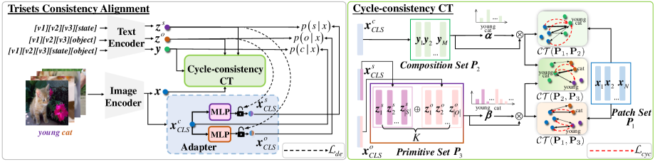
Figure 2: The overall framework of the proposed TsCA (zoom-in for more details).

Methodology

The proposed model aims to solve the CZSL from fine-grained alignments under the CT framework, where images are viewed as three discrete distributions over the image, composition, and primitive spaces. A novel consistency-aware CT is further developed to explore deeper interactions of these three domains. In this section, we start with the task of CZSL, and then introduce how to formulate CZSL as a CT problem in detail. The framework of our approach is shown in Fig. 2.

Problem Formulation

Given state set $\mathcal{S}=\{s_{0},s_{1},...,s_{|\mathcal{S}|}\}$ together with object set $\mathcal{O}=\{o_{0},o_{1},...,o_{|\mathcal{O}|}\}$ , we can define the label space with their Cartesian product, $\mathcal{C}=\mathcal{S}\times\mathcal{O}$. Then $\mathcal{C}$ can be divided into two disjoint label subsets such that $\mathcal{C}^{se}\in\mathcal{C}$, $\mathcal{C}^{us}\in\mathcal{C}$, and $\mathcal{C}^{se}\cap\mathcal{C}^{us}=\emptyset$ where $\mathcal{C}^{se}$ and $\mathcal{C}^{us}$ are the set of the seen and unseen classes respectively. Specifically, during the training phase, $\mathcal{C}^{se}$ are used to train a discriminative model $\mathcal{M}:\mathcal{X}\overrightarrow{\mathcal{missing}}{C}^{se}$ from the input image space to candidate composition label set. At inference time, the model is expected to predict unseen compositions in the test sample space, i.e.,$\mathcal{M}:\mathcal{X}\overrightarrow{\mathcal{missing}}{C}^{test}$. In this paper, we follow the setting of Generalized ZSL (Xian et al. 2017), considering testing samples contain both seen and unseen compositions. In general, in the closed-world evaluation, only the known composition space of test samples is required as $\mathcal{C}^{test}=\mathcal{C}^{se}\cup\mathcal{C}^{us}$. For the open-world evaluation (Karthik, Mancini, and Akata 2022a), the model has to consider all possible permutations of the state-object pairs, i.e., $\mathcal{C}^{test}=\mathcal{C}$.

Image as Three Sets

Built upon the pre-trained CLIP and with the soft prompt tuning technique, our TsCA represents an image as three sets: visual patch set ${\bf P}_{1}$, textual composition set ${\bf P}_{2}$, and primitive set ${\bf P}_{3}$. These sets capture the multimodal features of the same content from different semantic domains, acting as a fundamental role in the fine-grained alignments.

Patch Set.

For an input image $x$, CLIP first splits it into $N$ non-overlapping patches evenly and then feeds them (with a [CLS] token inserted) into the image encoder to extract the embedding of the [CLS] token $\boldsymbol{x}^{c}_{CLS}$ and the patch features $\boldsymbol{x}=\{\boldsymbol{x}_{n}|_{n=1}^{N}\}\in\mathbb{R}^{d\times N}$, where $\boldsymbol{x}_{n}\in\mathbb{R}^{d}$ denotes the embedding of patch $n$ with the embedding dimension being $d$. Naturally, the discrete probability distribution over the patch set can be formulated as:

$${\bf P}_{1}=\sum_{n=1}^{N}\theta_{n}\delta_{\boldsymbol{x}_{n}},\quad\theta_{n}=\frac{1}{N},$$ (1)

where $\delta$ denotes the Dirac delta function. We view all the patches equally and employ the Uniform distribution to model the patch weight $\boldsymbol{\theta}$. Note that ${\bf P}_{1}$ collects the detailed visual features of the local region, thereby bringing benefits to discriminative representation learning, especially when different concepts require emphasis on distinct areas within the input images. Besides, the [CLS] visual token $\boldsymbol{x}_{CLS}^{c}$ is also learned, serving as the global representation, which is often used as the image feature to downstream tasks (Zhou et al. 2022). Here, we consider it as the visual prior that constructs subsequent textual sets.

Composition Set.

In the textual domain, we build composition labels into a learnable soft prompt [v1][v2][v3][state][object], where [v] is the prefix vectors, and [state][object] denote the state and object name, respectively. Then, the prompt will be fed into the text encoder to obtain textual representations $\boldsymbol{y}=\{\boldsymbol{y}_{m}|_{m=1}^{M}\}\in\mathbb{R}^{d\times M}$, where $M$ is the number of training compositions. To embrace the variety of content and minimize the cross-modal disparities, we follow previous work (Huang et al. 2024) and incorporate a residual component obtained through a cross-attention mechanism (Vaswani 2017) with patch embeddings (we here still use $\boldsymbol{y}$ as the output compositions):

$$\boldsymbol{y}=\text{Cross-Att}(\boldsymbol{y}^{in},\boldsymbol{x},\boldsymbol{x})+\boldsymbol{y}^{in},$$ (2)

where $\boldsymbol{y}^{in}$ denotes the input compositions. Cross-Att is the cross-attention layer with the query $\boldsymbol{y}^{in}$, key $\boldsymbol{x}$, and value $\boldsymbol{x}$ as inputs, and outputs the fused features. As a result, the composition set can be viewed as:

$${\bf P}_{2}=\sum_{m=1}^{M}\alpha_{m}\delta_{\boldsymbol{y}_{m}},\quad\boldsymbol{\alpha}=\sigma(\boldsymbol{y}^{T}\boldsymbol{x}^{c}_{CLS}),$$ (3)

where $\sigma$ denotes the softmax function. We calculate the composition weights $\boldsymbol{\alpha}$ via the semantic similarity of the composition label and visual feature. This helps ${\bf P}_{2}$ to focus on compositions that describe the input image well.

Primitive Set.

Unlike the composition set that focuses on global textual features, the primitive set aims to explore the disentangled state and object representations. Motivated by the recent multi-path paradigms, we learn the corresponding primitive representations through [v1][v2][v3][state] and [v1][v2][v3][object], with the outputs denoted as $\boldsymbol{z}^{s}\in\mathbb{R}^{d\times{|\mathcal{S}|}}$ and $\boldsymbol{z}^{o}\in\mathbb{R}^{d\times{|\mathcal{O}|}}$ respectively. The corresponding probability weights are calculated as:

$$\boldsymbol{\beta}^{s}=\sigma(({\boldsymbol{z}^{s}})^{T}\boldsymbol{x}^{s}_{CLS}),\quad\boldsymbol{\beta}^{o}=\sigma(({\boldsymbol{z}^{o}})^{T}\boldsymbol{x}^{o}_{CLS}),$$ (4)

where $\boldsymbol{x}^{s}_{CLS}$ and $\boldsymbol{x}^{o}_{CLS}$ are two adapted visual features, which can be obtained via a lightweight adapter $g$:

$$[\boldsymbol{x}^{s}_{CLS},\boldsymbol{x}^{o}_{CLS}]=g(\boldsymbol{x}^{c}_{CLS}),$$ (5)

where $g$ takes the image feature $\boldsymbol{x}^{c}_{CLS}$ as input, and outputs the state/object-relevant features, deriving unique visual representations. To complete the primitive set, we concatenate the feature points from both state and object labels as $\boldsymbol{z}=\{\boldsymbol{z}_{k}|_{k=1}^{K}\}\in\mathbb{R}^{d\times K}$, where $K=|\mathcal{S}|+|\mathcal{O}|$ is the total number of state and object labels. Like compositions that fuse the patch features with Eq. 2, $\boldsymbol{z}$ is fed into the same cross-attention layer:

$$\boldsymbol{z}=\text{Cross-Att}(\boldsymbol{z}^{in},\boldsymbol{x},\boldsymbol{x})+\boldsymbol{z}^{in}.$$ (6)

Finally, the primitive set can be expressed as:

$${\bf P}_{3}=\sum_{k=1}^{K}\beta_{k}\delta_{\boldsymbol{z}_{k}},\quad\boldsymbol{\beta}=\sigma(\boldsymbol{\beta}^{s}\oplus\boldsymbol{\beta}^{o}),$$ (7)

where $\oplus$ denotes the concatenation operation. Together with ${\bf P}_{2}$, these two sets provide primitive-composition textual knowledge for downstream alignment tasks.

Semantic Consistency Alignment

Based on the three carefully constructed sets of the input image, our TsCA formulates the CZSL task as fine-grained alignments under the consistency-aware CT framework, which consists of pairwise CT distance and cycle consistency regularization.

Pairwise CT Distance.

Given the source distribution ${\bf P}_{1}$ and the target distribution ${\bf P}_{2}$, CT measures the distance by calculating the total transport costs bidirectionally, leading to the forward CT and backward CT, respectively. Denoting $c(\boldsymbol{x}_{n},\boldsymbol{y}_{m})\geq 0$ as a cost function to define the difference between points $\boldsymbol{x}_{n}$ and $\boldsymbol{y}_{m}$, the forward CT is measured as the expected transport cost of transporting all points from ${\bf P}_{1}$ to the target ${\bf P}_{2}$ set, and the backward CT reverses the transport direction. Mathematically, the CT distance between ${\bf P}_{1}$ and ${\bf P}2$ can be expressed as:

$$\mathcal{CT}({\bf P}_{1},{\bf P}_{2})=\min_{\overrightarrow{{\bf T}}\overleftarrow{{\bf T}}}(\sum_{n,m}\overrightarrow{t}_{nm}c_{nm}+\sum_{m,n}\overleftarrow{t}_{mn}c_{mn}),$$ (8)

$$\mathrm{s.t.}\overrightarrow{{\bf T}}\mathds{1}^{N}=\boldsymbol{\theta},\overleftarrow{{\bf T}}\mathds{1}^{M}=\boldsymbol{\alpha},$$

where we employ the cosine distance as the cost function, i.e., the closer the patch $\boldsymbol{x}_{n}$ and composition $\boldsymbol{y}_{m}$ are, the lower the transport cost. $\mathds{1}^{M}$ is the $M$ dimensional vector of ones. ${\bf T}$ is called the transport plan, which is to be learned to minimize the total distance. The forward transport plan, e.g., $\overrightarrow{t}_{nm}$ in $\overrightarrow{{\bf T}}$ describes the transport probability from the source point $\boldsymbol{x}_{n}$ to target point $\boldsymbol{y}_{m}$:

$$\overrightarrow{t}_{nm}=\theta_{n}\frac{\alpha_{m}e^{s_{\psi}(\boldsymbol{x}_{n},\boldsymbol{y}_{m})}}{\sum_{m^{\prime}=1}^{M}\alpha_{m}{{}^{\prime}}e^{s_{\psi}(\boldsymbol{x}_{n},\boldsymbol{y}_{m^{\prime}})}},$$ (9)

where $s_{\psi}$ denotes the similarity function with learnable parameter $\psi$, and we specify it as $s_{\psi}(\boldsymbol{x}_{n},\boldsymbol{y}_{m})=\frac{\boldsymbol{x}_{n}^{T}\boldsymbol{y}_{m}}{\text{exp}(\psi)}$. That is, the patch $\boldsymbol{x}_{n}$ will transport with higher probability if the composition $\boldsymbol{y}_{m}$ shares similar semantics with it. Similarly, we have the backward transport expressed as:

$$\overleftarrow{t}_{mn}=\alpha_{m}\frac{\theta_{n}e^{s_{\psi}(\boldsymbol{y}_{m},\boldsymbol{x}_{n})}}{\sum_{n^{\prime}=1}^{N}\theta_{n^{\prime}}e^{s_{\psi}(\boldsymbol{y}_{m},\boldsymbol{x}_{n^{\prime}})}}.$$ (10)

More interestingly, the definition in Eq. 9- 10 naturally satisfies the constraint in Eq. 8, simplifying the CT optimization.

By combining ${\bf P}_{1}$, ${\bf P}_{2}$, and ${\bf P}_{3}$ pairwise, we extend CT to the CZSL scenario and denote the total CT distances as:

$$\mathcal{CT}=\mathcal{CT}({\bf P}_{1},{\bf P}_{2})+\mathcal{CT}({\bf P}_{1},{\bf P}_{3})+\mathcal{CT}({\bf P}_{2},{\bf P}_{3}),$$ (11)

where the first two terms facilitate cross-domain alignments but focus on different semantic levels. $\mathcal{CT}({\bf P}_{1},{\bf P}_{2})$ takes the patch set and composition set as inputs and aims to find compositional visuals that match its textual label. While $\mathcal{CT}({\bf P}_{1},{\bf P}_{3})$ pays more attention to primitive alignment. Intuitively, the primitive set provides decoupled textual guidance, and it helps the model extract patches that contain the state or object-relevant visuals, which will improve the fine-grained predictions. Moving beyond the vision-language alignments, the last term attempts to explore the intra-modal interactions. $\mathcal{CT}({\bf P}_{2},{\bf P}_{3})$ optimizes the composition and its primitives to be semantically close in the embedding space, showing linguist coherence.

Cycle Consistency Regularization.

Due to the independent operation in Eq. 11, pairwise CTs may lead to potential inconsistencies and inefficiencies, as they fail to fully capture the global relationships among all sets involved. Cycle consistency, which has been extensively explored in domains such as image matching (Bernard et al. 2019), multi-graph alignment (Wang, Yan, and Yang 2021), and 3D pose estimation (Dong et al. 2019), offers a natural solution to this problem. By enforcing a closed-loop structure, cycle consistency can enhance the coherence of semantic relationships across all sets, ensuring more consistent and efficient alignment. Here, we denote the probability of the composition set being self-mapping back to its initial state as:

$${{\bf T}}_{22}=\overrightarrow{{\bf T}}_{23}\cdot\overrightarrow{{\bf T}}_{31}\cdot\overrightarrow{{\bf T}}_{12},$$ (12)

where $\overrightarrow{{\bf T}}_{23}$ denotes the transport plan from source ${\bf P}_{2}$ to target ${\bf P}_{3}$. This guarantees each label is transferred with a probability of 1 during transportation among three sets. For a given input, the corresponding point from the composition set first interacts with key patches in the patch set, then moves to the relevant state and object points within the primitive set, and finally returns to the composition set. Accordingly, we derive the cycle-consistency constraint by:

$$\mathcal{L}_{cyc}=\sum_{m=1}^{M}\boldsymbol{y}^{c}_{m}({\bf T}_{22}-\boldsymbol{I}),$$ (13)

where $\boldsymbol{y}^{c}_{m}$ denotes the one-hot binary label vector of the input image. For one thing, such a closed-loop transport constraint establishes a close link between independent pairwise CTs, which supports maintaining semantic consistency throughout the CT transport process. For another, it facilitates more robust composition representation learning, enhancing the model’s accuracy.

Primitive Decoupler.

In light of the intricate entanglement between attributes and objects within an image, we devise a decoupling loss with the idea that visual representation $\boldsymbol{x}^{s}_{CLS}$ and $\boldsymbol{x}^{o}_{CLS}$ can be seen as state-expert and object-expert if their paired sub-concepts fail to be inferred:

$$\mathcal{L}_{de}=\left\|cos(\boldsymbol{x}^{s}_{CLS},\boldsymbol{z}^{o}_{gt})\right\|+\left\|cos(\boldsymbol{x}^{o}_{CLS},\boldsymbol{z}^{s}_{gt})\right\|,$$ (14)

where $\boldsymbol{z}^{o}_{gt}$ and $\boldsymbol{z}^{s}_{gt}$ are textual representations for the ground-truth object class and attribute class, respectively. By mitigating the entanglement among visual representations, TsCA enhances its capacity to pinpoint correlative image representations that align with specific knowledge, thereby offering guidance on the textual sets prior and playing a complementary role in deriving a more accurate composition during inference.

Tranining and Inference

Training Objectives.

Recalling that the probability weights $\boldsymbol{\alpha}$, $\boldsymbol{\beta}^{s}$, and $\boldsymbol{\beta}^{o}$, calculated during the construction of the three sets, capture the semantic similarity between the visual image and the corresponding textual features, this naturally defines the probability for predicting the labels of state $s$, object $o$, and composition $c$ for the image $x$:

$$p(s|x)=\boldsymbol{\beta}^{s},\quad p(o|x)=\boldsymbol{\beta}^{o},\quad p(c|x)=\boldsymbol{\alpha}$$ (15)

Then the classification losses are given by:

$$\left\{\begin{matrix}\mathcal{L}_{s}=-\frac{1}{|\mathcal{X}|}{\sum_{\hat{x}\in\mathcal{X}}\text{log}p(s|x)}\\ \mathcal{L}_{o}=-\frac{1}{|\mathcal{X}|}{\sum_{\hat{x}\in\mathcal{X}}\text{log}p(o|x)}\\ \mathcal{L}_{c}=-\frac{1}{|\mathcal{X}|}{\sum_{\hat{x}\in\mathcal{X}}\text{log}p(c|x)}\end{matrix}\right..$$ (16)

Let $\mathcal{L}_{base}=\mathcal{L}_{c}+\mathcal{L}_{s}+\mathcal{L}_{o}$, the overall training loss is defined as follows:

$$\mathcal{L}=\lambda_{0}\mathcal{L}_{base}+\lambda_{1}\mathcal{CT}+\lambda_{2}\mathcal{L}_{cyc}+\lambda_{3}\mathcal{L}_{de},$$ (17)

where $\lambda_{\text{-}}$ are hyper-parameters to balance the losses. Like the previous works, the first term is our base classification loss. It will be used to predict the final label via a combined strategy during the inference. In addition, it helps to construct increasingly coherent textual sets as the loss decreases. The last three terms act as semantic regularization, which guides the learning process from various domain experts.

Inference.

With multi-path union, the prediction results of states and objects can be incorporated to assist the composition branch. Formally, the integrated composition probability can be denoted as:

$$\tilde{p}(c|x)=\gamma p(c|x)+(1-\gamma)(p(s|x)\times p(o|x)),$$ (18)

where $\gamma$ balances the contributions of primitive prediction and composition prediction in multi-path learning.

Additionally, we apply a single CT computation to filter out infeasible compositions that might be present in the open-world setting. Concretely, we calculate the bidirectional transport plans between primitives and compositions as their feasible scores, and discarded less relevant pairs by a threshold $T$ in :

$$\mathcal{C}^{test^{{}^{\prime}}}=\left\{c=(s,o):{\overrightarrow{t}_{cs}}{\overrightarrow{t}_{co}}+{\overleftarrow{t}_{sc}}{\overleftarrow{t}_{oc}}<T\right\}.$$ (19)

This strategy reduces the search space and increases performance simultaneously.

Experiment

Experimental Settings

Datasets. The proposed TsCA is evaluated on three real-world CZSL benchmark datasets: MIT-states(Isola, Lim, and Adelson 2015), UT-Zappos(Yu and Grauman 2014) and C-GQA (Naeem et al. 2021). MIT-States comprises images of naturally occurring objects, with each object characterized by an accompanying adjective description. It comprises 53,753 images depicting 115 states and 245 objects. UT-Zappos is a fine-grained dataset consisting of different kinds of shoes with texture attributes, totaling 16 states and 12 objects. C-GQA, derived from the Stanford GQA dataset (Hudson and Manning 2019), features 453 states and 870 objects with over 9,500 compositions, making it the most pairs dataset for CZSL. We follow the split suggested by the previous work (Purushwalkam et al. 2019) to ensure fair comparisons and detailed statistics can be found in Tab. 1.

Table 1: Statistics of datasets

Dataset	Train		Validation			Test
	|Ys|	|X|	|Ys|	|Yu|	|X|	|Ys|	|Yu|	|X|
MIT-States	1262	30338	300	300	10420	400	400	12995
UT-Zappos	83	22998	15	15	3214	18	18	2914
C-GQA	5592	26920	1252	1040	7280	888	923	5098

Table 2: CZSL comparisons in the close-world setting. The best results are in bold. The second best results are in blue.

	MIT-States				UT-Zappos				C-GQA
Method	S	U	H	AUC	S	U	H	AUC	S	U	H	AUC
CLIP (Radford et al. 2021)	30.2	46.0	26.1	11.0	15.8	49.1	15.6	5.0	7.5	25.0	8.6	1.4
CoOp (Zhou et al. 2022)	34.4	47.6	29.8	13.5	52.1	49.3	34.6	18.8	20.5	26.8	17.1	4.4
PromptCompVL (Xu et al. 2022)	48.5	47.2	35.3	18.3	64.4	64.0	46.1	32.2	——	——	——	——
CSP (Nayak, Yu, and Bach 2023)	46.6	49.9	36.3	19.4	64.2	66.2	46.6	33.0	28.8	26.8	20.5	6.2
HPL (Wang et al. 2023a)	47.5	50.6	37.3	20.2	63.0	68.8	48.2	35.0	30.8	28.4	22.4	7.2
GIPCOL (Xu, Chai, and Kordjamshidi 2024)	48.5	49.6	36.6	19.9	65.0	68.5	48.8	36.2	31.9	28.4	22.5	7.1
DFSP (i2t) (Lu et al. 2023)	47.4	52.4	37.2	20.7	64.2	66.4	45.1	32.1	35.6	29.3	24.3	8.7
DFSP (BiF) (Lu et al. 2023)	47.1	52.8	37.7	20.8	63.3	69.2	47.1	33.5	36.5	32.0	26.2	9.9
DFSP (t2i) (Lu et al. 2023)	46.9	52.0	37.3	20.6	66.7	71.7	47.2	36.0	38.2	32.0	27.1	10.5
PLID (Bao et al. 2023)	49.7	52.4	39.0	22.1	67.3	68.8	52.4	38.7	38.8	33.0	27.9	11.0
Troika (Huang et al. 2024)	49.0	53.0	39.3	22.1	66.8	73.8	54.6	41.7	41.0	35.7	29.4	12.4
CDS-CZSL (Li et al. 2024)	50.3	52.9	39.2	22.4	63.9	74.8	52.7	39.5	38.3	34.2	28.1	11.1
Retrieval-Augmented (Jing et al. 2024)	50.0	53.3	39.2	22.5	69.4	72.8	56.5	44.5	45.6	36.0	32.0	14.4
TsCA	51.2	52.9	39.9	23.0	68.6	74.3	58.4	45.2	42.9	38.9	32.5	14.6

Table 3: CZSL comparisons in the open-world setting. We use ‘w’ and ‘w/o’ to distinguish models adopting filtering strategy to filter unfeasible compositions. The best results are in bold. The second best results are in blue.

	MIT-States				UT-Zappos				CGQA
Method	S	U	H	AUC	S	U	H	AUC	S	U	H	AUC
CLIP (Radford et al. 2021)	30.1	14.3	12.8	3.0	15.7	20.6	11.2	2.2	7.5	4.6	4.0	0.3
CoOp (Zhou et al. 2022)	34.6	9.3	12.3	2.8	52.1	31.5	28.9	13.2	21.0	4.6	5.5	0.7
PromptCompVL (Xu et al. 2022)	48.5	16.0	17.7	6.1	64.6	44.0	37.1	21.6	——	——	——	——
CSP (Nayak, Yu, and Bach 2023)	46.3	15.7	17.4	5.7	64.1	44.1	38.9	22.7	28.7	5.2	6.9	1.2
HPL (Wang et al. 2023a)	46.4	18.9	19.8	6.9	63.4	48.1	40.2	24.6	30.1	5.8	7.5	1.4
GIPCOL (Xu, Chai, and Kordjamshidi 2024)	48.5	16.0	17.9	6.3	65.0	45.0	40.1	23.5	31.6	5.5	7.3	1.3
DFSP (i2t) (Lu et al. 2023)	47.2	18.2	19.1	6.7	64.3	53.8	41.2	26.4	35.6	6.5	9.0	2.0
DFSP (BiF) (Lu et al. 2023)	47.1	18.1	19.2	6.7	63.5	57.2	42.7	27.6	36.4	7.6	10.6	2.4
DFSP (t2i) (Lu et al. 2023)	47.5	18.5	19.3	6.8	66.8	60.0	44.0	30.3	38.3	7.2	10.4	2.4
PLID (Bao et al. 2023)	49.1	18.7	20.0	7.3	67.6	55.5	46.6	30.8	39.1	7.5	10.6	2.5
Troika (Huang et al. 2024)	48.8	18.7	20.1	7.2	66.4	61.2	47.8	33.0	40.8	7.9	10.9	2.7
CDS-CZSL (Li et al. 2024)	49.4	21.8	22.1	8.5	64.7	61.3	48.2	32.3	37.6	8.2	11.6	2.7
Retrieval-Augmented (Jing et al. 2024)	49.9	20.1	21.8	8.2	69.4	59.4	47.9	33.3	45.5	11.2	14.6	4.4
TsCA (w/o filter)	50.7	21.4	21.9	8.6	67.6	63.5	52.0	36.1	43.2	11.2	14.6	4.3
TsCA (w filter)	50.8	21.5	22.0	8.7	68.3	63.8	52.5	36.7	43.6	11.3	14.7	4.5

Metrics. Following the common practice of prior works (Lu et al. 2023), we utilize the standard evaluation protocols and assessed all results using four metrics in both closed-world and open-world scenarios. Concretely, S measures the best seen accuracy when calibration bias is $+\infty$ and U denotes the accuracy specifically for unseen compositions when the bias is $-\infty$. To provide an overall performance measure on both seen and unseen pairs, we also report the area under the seen-unseen accuracy curve (AUC) by varying the calibration bias from $+\infty$ to $-\infty$ and identify the point that achieves the best harmonic mean (H) between the seen and unseen accuracy. Among these, H and AUC are the core metrics for comprehensively evaluating the model.

Implementation Details. The proposed TsCA and all baselines are implemented with a per-trained CLIP ViT-L/14 model in PyTorch (Paszke et al. 2019). For the UT-Zappos, the hyper-parameters $\lambda_{0}$, $\lambda_{1}$, $\lambda_{2}$, $\lambda_{3}$ in losses are set as 1, 0.1, 0.1, and 1. For the MIT-States, the hyper-parameters are set as 1, 0.01, 0.05, and 0.01. For the CGQA, the hyper-parameters are set as 1, 0.01, 0.03, and 0.01. During inference, $\gamma$ is set to 0.8 for UT-Zappos and 0.4 for MIT-States and C-GQA in the closed-world scenario and is adjusted to 0.4, 0.3, and 0.2 for each of the datasets in the open-world setting. The primitive adapters consist of two individual single-layer MLPs. All experiments are performed on a single NVIDIA RTX A6000 GPU. Please refer to the appendix for more details.

Comparision with State-of-the-Arts

We compare our TsCA with the most recent CZSL methods. The results are shown in Tab. 2 and Tab 3. On the closed-world setting, TsCA exceeds the previous SOTA methods on all datasets in core metrics. Specifically, it yields improvements of 0.6% on MIT-States, 1.9% on UT-Zappos, and 0.5% on C-GQA in H over the second-best methods. It also attains considerable gains in AUC with increases of 0.5%, 0.7%, and 0.2%, respectively. Notably, the advantage of UT-Zappos is more significant, suggesting that the fine-grained nature of UT-Zappos can better align with TsCA’s ability to achieve precise alignment across local visual features and textual representations. Similarly, the results in the open-world setting are also promising. Our TsCA attains the highest AUC across all datasets , with the scores of 8.7% ,36.7% and 4.5%. It should be noted that the CT-based filtering strategy contributes to the improvements in this challenging setting. All numerical results substantiate our motivation to empower the model to capture semantic consistency among the image-composition-primitive interactions.

Table 4: Ablation results for each component on UT-Zappos in the closed-world setting.

	$\mathcal{L}_{de}$	$\text{CT}_{{\bf C}}$	$\mathcal{L}_{cyc}$	S	U	H	AUC
1				65.7	73.5	54.4	40.8
2	✓			68.2	73.9	56.8	44.3
3		✓		67.0	74.1	56.7	43.8
4		✓	✓	67.7	74.4	57.3	44.6
5	✓	✓		68.5	74.5	57.6	44.9
6	✓	✓	✓	68.6	74.3	58.4	45.1

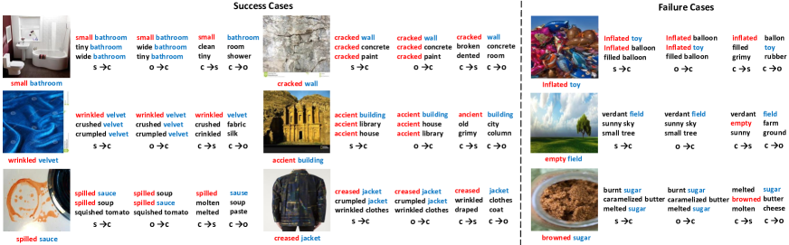
Figure 3: Qualitative results of the intra-modal transport plans on the MIT-States. For each sample, we show an image with the ground-truth composition, with the state indicated in red and the object in blue. The top-3 predictions are presented in two formats: from the primitive class to the composition set in the first two columns, and from the composition label to the primitive set in the third and fourth columns. The annotations ‘p’,‘s’, ‘o’, and ‘c’ correspond to patch, state, object, and composition, respectively.

Ablation Study

We empirically verify the effectiveness of each component in TsCA on UT-Zappos by comparing it against five variants. The results, seen in Tab. 4, illustrate several observations: 1) The baseline model, i.e., removes the consistency-aware CT module and decoupler loss, shows the lowest performance. 2) Introducing either pairwise CT loss or decoupler loss on top of the baseline model significantly boosts all metrics. Notably, both primitive decoupler and cycle-consistency constraint positively contribute to pairwise CT. The former improves the quality of the textual sets, while the latter ensures semantic consistency during the transport chain, each leading to further enhancements in the model’s effectiveness. 3) Combining the strengths of all components, our complete model achieves the best performance in terms of H and AUC.

To demonstrate the effectiveness of cycle-consistency, we draw the self-mapping matrix of the composition set for our full model on test data in Fig. 4. Though degradation occurs in the unseen pair positions, the results still exhibit a close similarity to the identity matrix.

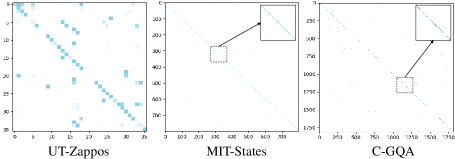
Figure 4: Cycle-consistency (zoom-in for more details).

Qualitative Results

We further provide some visualization examples of transport plans learned in our TsCA. Recalling that the columns $\overleftarrow{{\bf T}}_{21}$ and $\overleftarrow{{\bf T}}_{31}$ depict how likely the corresponding textual semantics are transported to each visual patch. We convert each transport plan into heatmaps and resize them to combine with the raw image at Fig. 5. We observe that different prompts from multi-path tend to align different patch regions, each of which contributes to the final prediction. For example, in the first row, the state branch emphasizes the wet fur, the object branch highlights the nose and mouth as key features for recognizing a cat, while the composition branch provides a more comprehensive focus on both aspects.

Moving beyond the visualization of cross-modal alignment, $\overleftarrow{{\bf T}}_{32}$ and $\overrightarrow{{\bf T}}_{23}$ also grant us access to intra-modal components, prompting an exploration of the interplay between compositions and primitives in an interpretable form. Fig. 3 presents the top-3 transport retrieval results for bidirectional transfers between the composition and primitive sets. Note that our model can both retrieve the correct composition from the primitive set, and also adeptly performs the inverse mapping of conceptual pairs. Besides, all top-3 retrieval results not only ensure the rationality of the state-object combination but also conform to the description of the images. We also present some failure cases. Interestingly, even when incorrect, the retrieved labels still capture the content of the given images, demonstrating the effectiveness of our TsCA.

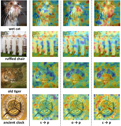
Figure 5: Visualization of the cross-modal transport plans on the Mit-States. Columns 1-3 represent the transport from the ground-truth state and object points in the primitive set, as well as the composition points in the composition set, to the patch set.

Conclusion

In this paper, we revisit compositional generalization in CZSL through a conditional transport perspective. We explore pairwise CTs between the local visual features of images and two textual label sets within a multi-path paradigm. We then introduce cycle-consistency as a link to bond all sets, promoting robust learning. The primitive decoupler further improved accuracy and decoupled global primitive visual representations during prediction. Benefited from transport plan between primitive set and composition set, this approach successfully narrowed the composition search space by excluding unfeasible pairs during inference. Extensive experiments across three benchmarks consistently demonstrate the superiority of TsCA. Comprehensive ablation studies and visualizations confirm our motivation and the essential role of each component. With its inherent flexibility and simplicity, we hope our work inspires innovative ideas for future research.

Appendix

A. Implementation Details

In Table. 5, we list the hyper-parameters that differ on each dataset and determined with the validation performance. Considering that the visual content of the same sub-concept can change significantly when faced with different state-object combinations-such as ’old dog’ versus ’old house’- we introduced a cross-modal attention(Cross-Att) to refine primitive set and composition set. For the setting of the number of Cross-Att layers, we followed (Huang et al. 2024). During training, we use the Adam optimizer over all datasets.

Table 5: Hyper-parameters for different datasets.

Hyper-parameter	MIT-States	UT-Zappos	CGQA
Learning rate	10-4	5$\times 10^{-4}$	1.5$\times 10^{-5}$
Batch size	32	32	4
Number of epochs	10	10	10
Weight decay	10-5	10-5	10-5
Number of Cross-Att layers	3	2	2

During inference, the filtering threshold T is calibrated based on the performance on the validation set. We report the statistics of T in Table 6.

Table 6: Statistics of filtering threthold T.

T	MIT-States	UT-Zappos	CGQA
value	0.43	0.035	0.29
unfeasible pairs	282	3	2784

B. Further Experiments of Hyper-Parameter

In this section, we focus on the analysis of the effects arising from the inference weighting coefficient configurations. In Figure 6, we vary the weight coefficient of the composition branch, $\gamma$, from 0 to 1 in intervals of 0.2. We found that for UT-Zappos, prioritizing compositional learning in the closed-world setting leads to the best results in both AUC and HM. However, in the open-world setting, there is a tendency to favor the primitive branches over the composition branch. Furthermore, both scenarios exhibit a significant performance drop when $\gamma$ equals 0, indicating the necessity of primitive prompt learning and primitive set construction used by TsCA.

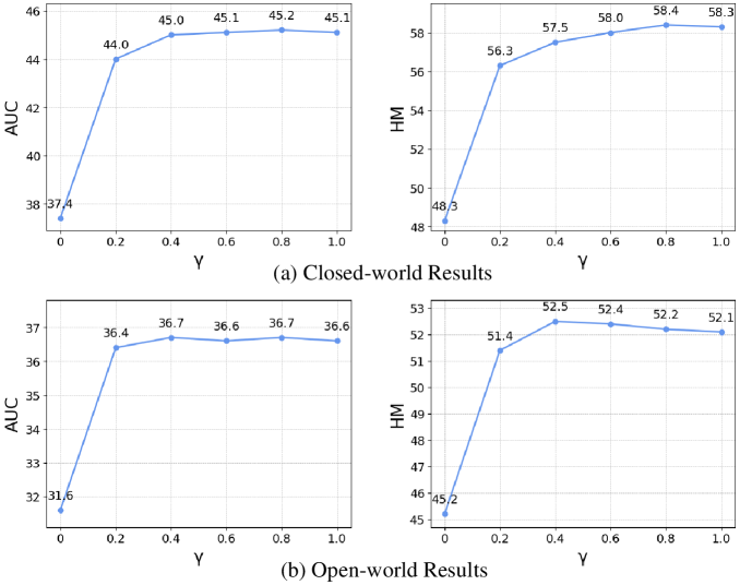
Figure 6: Influence of $\gamma$ on UT-Zappos.

C. Additional Comparison Results

Following previous work(Huang et al. 2024; Li et al. 2024; Jing et al. 2024), we included comparisons between CLIP-based methods and existing CZSL methods using a pre-trained ResNet-18 backbone to provide a more comprehensive comparison. We report the close-world results in Table 7 and the open-world results in Table 8, respectively. From these comparisons, we observe that CLIP-based methods have higher performance ceilings, and our approach outperforms all the baselines in most cases, showing the efficiency of the fine-grained alignments of the image-composition-primitive sets.

Table 7: Comparison with state-of-the-art baselines on CZSL datasets in the close-world setting. The best results are in bold. The second best results are in blue.

	MIT-States				UT-Zappos				C-GQA
Method	S	U	H	AUC	S	U	H	AUC	S	U	H	AUC
CompCos (Mancini et al. 2021)	25.3	24.6	16.4	4.5	59.8	62.5	43.1	28.7	28.1	11.2	12.4	2.6
CGE (Naeem et al. 2021)	32.8	28.0	21.4	6.5	64.5	71.5	60.5	33.5	31.4	14.0	14.5	3.6
Co-CGE (Mancini et al. 2022)	32.1	28.3	20.0	6.6	62.3	66.3	48.1	33.9	33.3	14.9	14.4	4.1
CANet (Wang et al. 2023b)	29.0	26.2	17.9	5.4	61.0	66.3	47.3	33.1	30.0	13.2	14.5	3.4
CAPE (Khan et al. 2023)	32.1	28.0	20.4	6.7	62.3	68.5	49.5	35.2	33.0	16.4	16.3	4.6
ADE (Hao, Han, and Wong 2023)	——	——	——	——	63.0	64.3	51.1	35.1	35.0	17.7	18.0	5.2
CLIP (Radford et al. 2021)	30.2	46.0	26.1	11.0	15.8	49.1	15.6	5.0	7.5	25.0	8.6	1.4
CoOp (Zhou et al. 2022)	34.4	47.6	29.8	13.5	52.1	49.3	34.6	18.8	20.5	26.8	17.1	4.4
PromptCompVL (Xu et al. 2022)	48.5	47.2	35.3	18.3	64.4	64.0	46.1	32.2	——	——	——	——
CSP (Nayak, Yu, and Bach 2023)	46.6	49.9	36.3	19.4	64.2	66.2	46.6	33.0	28.8	26.8	20.5	6.2
HPL (Wang et al. 2023a)	47.5	50.6	37.3	20.2	63.0	68.8	48.2	35.0	30.8	28.4	22.4	7.2
GIPCOL (Xu, Chai, and Kordjamshidi 2024)	48.5	49.6	36.6	19.9	65.0	68.5	48.8	36.2	31.9	28.4	22.5	7.1
DFSP (i2t) (Lu et al. 2023)	47.4	52.4	37.2	20.7	64.2	66.4	45.1	32.1	35.6	29.3	24.3	8.7
DFSP (BiF) (Lu et al. 2023)	47.1	52.8	37.7	20.8	63.3	69.2	47.1	33.5	36.5	32.0	26.2	9.9
DFSP (t2i) (Lu et al. 2023)	46.9	52.0	37.3	20.6	66.7	71.7	47.2	36.0	38.2	32.0	27.1	10.5
PLID (Bao et al. 2023)	49.7	52.4	39.0	22.1	67.3	68.8	52.4	38.7	38.8	33.0	27.9	11.0
Troika (Huang et al. 2024)	49.0	53.0	39.3	22.1	66.8	73.8	54.6	41.7	41.0	35.7	29.4	12.4
CDS-CZSL (Li et al. 2024)	50.3	52.9	39.2	22.4	63.9	74.8	52.7	39.5	38.3	34.2	28.1	11.1
Retrieval-Augmented (Jing et al. 2024)	50.0	53.3	39.2	22.5	69.4	72.8	56.5	44.5	45.6	36.0	32.0	14.4
TsCA	51.2	52.9	39.9	23.0	68.6	74.3	58.4	45.2	42.9	38.9	32.5	14.6

Table 8: Comparison with state-of-the-art baslines on CZSL datasets in the open-world setting. We use ’w’ and ’w/o’ to distinguish models adopting filtering strategy to filter unfeasible compositions. The best results are in bold. The second best results are in blue.

	MIT-States				UT-Zappos				CGQA
Method	S	U	H	AUC	S	U	H	AUC	S	U	H	AUC
CompCos (Mancini et al. 2021)	25.4	10.0	8.9	1.6	59.3	46.8	36.9	21.3	28.4	1.8	2.8	0.4
CGE (Naeem et al. 2021)	32.4	5.1	6.0	1.0	61.7	47.7	39.0	23.1	32.7	1.8	2.9	0.5
Co-CGE (Mancini et al. 2022)	30.3	11.2	10.7	2.3	61.2	45.8	40.8	23.3	32.1	3.0	4.8	0.8
KG-SP (Karthik, Mancini, and Akata 2022b)	28.4	7.5	7.4	1.3	61.8	52.1	42.3	26.5	31.5	2.9	4.7	0.8
DRANet (Li et al. 2023c)	29.8	7.8	7.9	1.5	65.1	54.3	44.0	28.8	31.3	3.9	6.0	1.1
ADE (Hao, Han, and Wong 2023)	——	——	——	——	62.4	50.7	44.8	27.1	35.1	4.8	7.6	1.4
CLIP (Radford et al. 2021)	30.1	14.3	12.8	3.0	15.7	20.6	11.2	2.2	7.5	4.6	4.0	0.3
CoOp (Zhou et al. 2022)	34.6	9.3	12.3	2.8	52.1	31.5	28.9	13.2	21.0	4.6	5.5	0.7
PromptCompVL (Xu et al. 2022)	48.5	16.0	17.7	6.1	64.6	44.0	37.1	21.6	——	——	——	——
CSP (Nayak, Yu, and Bach 2023)	46.3	15.7	17.4	5.7	64.1	44.1	38.9	22.7	28.7	5.2	6.9	1.2
HPL (Wang et al. 2023a)	46.4	18.9	19.8	6.9	63.4	48.1	40.2	24.6	30.1	5.8	7.5	1.4
GIPCOL (Xu, Chai, and Kordjamshidi 2024)	48.5	16.0	17.9	6.3	65.0	45.0	40.1	23.5	31.6	5.5	7.3	1.3
DFSP (i2t) (Lu et al. 2023)	47.2	18.2	19.1	6.7	64.3	53.8	41.2	26.4	35.6	6.5	9.0	2.0
DFSP (BiF) (Lu et al. 2023)	47.1	18.1	19.2	6.7	63.5	57.2	42.7	27.6	36.4	7.6	10.6	2.4
DFSP (t2i) (Lu et al. 2023)	47.5	18.5	19.3	6.8	66.8	60.0	44.0	30.3	38.3	7.2	10.4	2.4
PLID (Bao et al. 2023)	49.1	18.7	20.0	7.3	67.6	55.5	46.6	30.8	39.1	7.5	10.6	2.5
Troika (Huang et al. 2024)	48.8	18.7	20.1	7.2	66.4	61.2	47.8	33.0	40.8	7.9	10.9	2.7
CDS-CZSL (Li et al. 2024)	49.4	21.8	22.1	8.5	64.7	61.3	48.2	32.3	37.6	8.2	11.6	2.7
Retrieval-Augmented (Jing et al. 2024)	49.9	20.1	21.8	8.2	69.4	59.4	47.9	33.3	45.5	11.2	14.6	4.4
TsCA (w/o filter)	50.7	21.4	21.9	8.6	67.6	63.5	52.0	36.1	43.2	11.2	14.6	4.3
TsCA (w filter)	50.8	21.5	22.0	8.7	68.3	63.8	52.5	36.7	43.6	11.3	14.7	4.5

D. More visualizations

For a more comprehensive qualitative analysis, we present the visualization results of cross-modal transportation plans between the composition and primitive sets on the MIT States and C-GQA datasets, as illustrated in Fig. 7 and Fig. 8. It is observed that TsCA’s top-1 retrieval consistently identifies the correct composition from the primitive set, while the top-2 and top-3 retrievals yield labels that are semantically close to the ground-truth labels. Besides, all top-3 retrieval results not only ensure the rationality of the state-object combination but also conform to the description of the images.

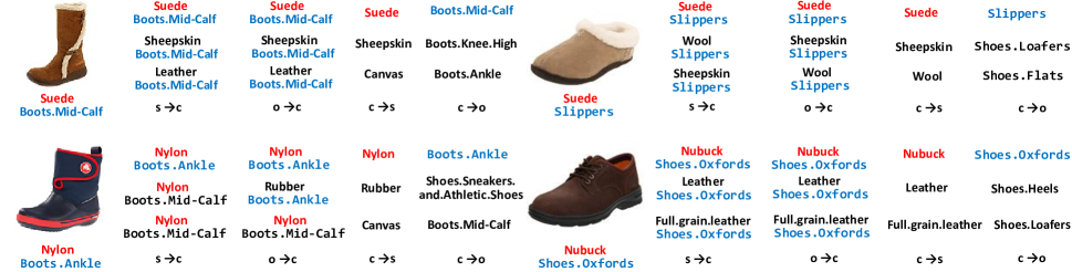
Figure 7: Qualitative results of the intra-modal transport plans on the UT-Zappos. The annotations ’p’,’s’, ’o’, and ’c’ correspond to patch, state, object, and composition, respectively.

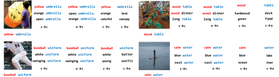
Figure 8: Qualitative results of the intra-modal transport plans on the C-GQA. The annotations ’p’,’s’, ’o’, and ’c’ correspond to patch, state, object, and composition, respectively.

References

- Bao et al. (2023) Bao, W.; Chen, L.; Huang, H.; and Kong, Y. 2023. Prompting language-informed distribution for compositional zero-shot learning. arXiv preprint arXiv:2305.14428.
- Bernard et al. (2019) Bernard, F.; Thunberg, J.; Swoboda, P.; and Theobalt, C. 2019. Hippi: Higher-order projected power iterations for scalable multi-matching. In Proceedings of the ieee/cvf international conference on computer vision, 10284–10293.
- Dong et al. (2019) Dong, J.; Jiang, W.; Huang, Q.; Bao, H.; and Zhou, X. 2019. Fast and robust multi-person 3d pose estimation from multiple views. In Proceedings of the IEEE/CVF conference on computer vision and pattern recognition, 7792–7801.
- Hao, Han, and Wong (2023) Hao, S.; Han, K.; and Wong, K.-Y. K. 2023. Learning attention as disentangler for compositional zero-shot learning. In Proceedings of the IEEE/CVF Conference on Computer Vision and Pattern Recognition, 15315–15324.
- Huang et al. (2024) Huang, S.; Gong, B.; Feng, Y.; Zhang, M.; Lv, Y.; and Wang, D. 2024. Troika: Multi-path cross-modal traction for compositional zero-shot learning. In Proceedings of the IEEE/CVF Conference on Computer Vision and Pattern Recognition, 24005–24014.
- Hudson and Manning (2019) Hudson, D. A.; and Manning, C. D. 2019. Gqa: A new dataset for real-world visual reasoning and compositional question answering. In Proceedings of the IEEE/CVF conference on computer vision and pattern recognition, 6700–6709.
- Huynh and Elhamifar (2020) Huynh, D.; and Elhamifar, E. 2020. Compositional zero-shot learning via fine-grained dense feature composition. Advances in Neural Information Processing Systems, 33: 19849–19860.
- Isola, Lim, and Adelson (2015) Isola, P.; Lim, J. J.; and Adelson, E. H. 2015. Discovering states and transformations in image collections. In Proceedings of the IEEE conference on computer vision and pattern recognition, 1383–1391.
- Jing et al. (2024) Jing, C.; Li, Y.; Chen, H.; and Shen, C. 2024. Retrieval-Augmented Primitive Representations for Compositional Zero-Shot Learning. In Proceedings of the AAAI Conference on Artificial Intelligence, volume 38, 2652–2660.
- Karthik, Mancini, and Akata (2022a) Karthik, S.; Mancini, M.; and Akata, Z. 2022a. KG-SP: Knowledge Guided Simple Primitives for Open World Compositional Zero-Shot Learning. 2022 IEEE/CVF Conference on Computer Vision and Pattern Recognition (CVPR), 9326–9335.
- Karthik, Mancini, and Akata (2022b) Karthik, S.; Mancini, M.; and Akata, Z. 2022b. Kg-sp: Knowledge guided simple primitives for open world compositional zero-shot learning. In Proceedings of the IEEE/CVF Conference on Computer Vision and Pattern Recognition, 9336–9345.
- Khan et al. (2023) Khan, M. G. Z. A.; Naeem, M. F.; Van Gool, L.; Pagani, A.; Stricker, D.; and Afzal, M. Z. 2023. Learning attention propagation for compositional zero-shot learning. In Proceedings of the IEEE/CVF Winter Conference on Applications of Computer Vision, 3828–3837.
- Li et al. (2023a) Li, L.; Chen, G.; Xiao, J.; and Chen, L. 2023a. Compositional zero-shot learning via progressive language-based observations. arXiv preprint arXiv:2311.14749.
- Li et al. (2023b) Li, M.; Wang, D.; Liu, X.; Zeng, Z.; Lu, R.; Chen, B.; and Zhou, M. 2023b. Patchct: Aligning patch set and label set with conditional transport for multi-label image classification. In Proceedings of the IEEE/CVF International Conference on Computer Vision, 15348–15358.
- Li et al. (2022) Li, X.; Yang, X.; Wei, K.; Deng, C.; and Yang, M. 2022. Siamese contrastive embedding network for compositional zero-shot learning. In Proceedings of the IEEE/CVF conference on computer vision and pattern recognition, 9326–9335.
- Li et al. (2024) Li, Y.; Liu, Z.; Chen, H.; and Yao, L. 2024. Context-based and Diversity-driven Specificity in Compositional Zero-Shot Learning. In Proceedings of the IEEE/CVF Conference on Computer Vision and Pattern Recognition, 17037–17046.
- Li et al. (2023c) Li, Y.; Liu, Z.; Jha, S.; and Yao, L. 2023c. Distilled reverse attention network for open-world compositional zero-shot learning. In Proceedings of the IEEE/CVF International Conference on Computer Vision, 1782–1791.
- Li et al. (2020) Li, Y.-L.; Xu, Y.; Mao, X.; and Lu, C. 2020. Symmetry and group in attribute-object compositions. 2020 IEEE. In CVF Conference on Computer Vision and Pattern Recognition (CVPR), 11313–11322.
- Liu et al. (2023) Liu, Z.; Li, Y.; Yao, L.; Chang, X.; Fang, W.; Wu, X.; and El Saddik, A. 2023. Simple primitives with feasibility-and contextuality-dependence for open-world compositional zero-shot learning. IEEE Transactions on Pattern Analysis and Machine Intelligence.
- Lu et al. (2023) Lu, X.; Guo, S.; Liu, Z.; and Guo, J. 2023. Decomposed soft prompt guided fusion enhancing for compositional zero-shot learning. In Proceedings of the IEEE/CVF Conference on Computer Vision and Pattern Recognition, 23560–23569.
- Mancini et al. (2021) Mancini, M.; Naeem, M. F.; Xian, Y.; and Akata, Z. 2021. Open world compositional zero-shot learning. In Proceedings of the IEEE/CVF conference on computer vision and pattern recognition, 5222–5230.
- Mancini et al. (2022) Mancini, M.; Naeem, M. F.; Xian, Y.; and Akata, Z. 2022. Learning graph embeddings for open world compositional zero-shot learning. IEEE Transactions on pattern analysis and machine intelligence, 46(3): 1545–1560.
- Misra, Gupta, and Hebert (2017) Misra, I.; Gupta, A.; and Hebert, M. 2017. From red wine to red tomato: Composition with context. In Proceedings of the IEEE Conference on Computer Vision and Pattern Recognition, 1792–1801.
- Naeem et al. (2021) Naeem, M. F.; Xian, Y.; Tombari, F.; and Akata, Z. 2021. Learning graph embeddings for compositional zero-shot learning. In Proceedings of the IEEE/CVF Conference on Computer Vision and Pattern Recognition, 953–962.
- Nagarajan and Grauman (2018) Nagarajan, T.; and Grauman, K. 2018. Attributes as operators: factorizing unseen attribute-object compositions. In Proceedings of the European Conference on Computer Vision (ECCV), 169–185.
- Nayak, Yu, and Bach (2023) Nayak, N. V.; Yu, P.; and Bach, S. H. 2023. Learning to Compose Soft Prompts for Compositional Zero-Shot Learning. In The Eleventh International Conference on Learning Representations, ICLR 2023, Kigali, Rwanda, May 1-5, 2023. OpenReview.net.
- Paszke et al. (2019) Paszke, A.; Gross, S.; Massa, F.; Lerer, A.; Bradbury, J.; Chanan, G.; Killeen, T.; Lin, Z.; Gimelshein, N.; Antiga, L.; et al. 2019. Pytorch: An imperative style, high-performance deep learning library. Advances in neural information processing systems, 32.
- Purushwalkam et al. (2019) Purushwalkam, S.; Nickel, M.; Gupta, A.; and Ranzato, M. 2019. Task-driven modular networks for zero-shot compositional learning. In Proceedings of the IEEE/CVF International Conference on Computer Vision, 3593–3602.
- Radford et al. (2021) Radford, A.; Kim, J. W.; Hallacy, C.; Ramesh, A.; Goh, G.; Agarwal, S.; Sastry, G.; Askell, A.; Mishkin, P.; Clark, J.; et al. 2021. Learning transferable visual models from natural language supervision. In International conference on machine learning, 8748–8763. PMLR.
- Saini, Pham, and Shrivastava (2022) Saini, N.; Pham, K.; and Shrivastava, A. 2022. Disentangling visual embeddings for attributes and objects. In Proceedings of the IEEE/CVF Conference on Computer Vision and Pattern Recognition, 13658–13667.
- Tanwisuth et al. (2021) Tanwisuth, K.; Fan, X.; Zheng, H.; Zhang, S.; Zhang, H.; Chen, B.; and Zhou, M. 2021. A prototype-oriented framework for unsupervised domain adaptation. Advances in Neural Information Processing Systems, 34: 17194–17208.
- Tanwisuth et al. (2023) Tanwisuth, K.; Zhang, S.; Zheng, H.; He, P.; and Zhou, M. 2023. POUF: Prompt-oriented unsupervised fine-tuning for large pre-trained models. In International Conference on Machine Learning, 33816–33832. PMLR.
- Tian et al. (2023) Tian, L.; Feng, J.; Chai, X.; Chen, W.; Wang, L.; Liu, X.; and Chen, B. 2023. Prototypes-oriented transductive few-shot learning with conditional transport. In Proceedings of the IEEE/CVF International Conference on Computer Vision, 16317–16326.
- Vaswani (2017) Vaswani, A. 2017. Attention is all you need. arXiv preprint arXiv:1706.03762.
- Wang et al. (2022) Wang, D.; Guo, D.; Zhao, H.; Zheng, H.; Tanwisuth, K.; Chen, B.; and Zhou, M. 2022. Representing mixtures of word embeddings with mixtures of topic embeddings. arXiv preprint arXiv:2203.01570.
- Wang et al. (2023a) Wang, H.; Yang, M.; Wei, K.; and Deng, C. 2023a. Hierarchical Prompt Learning for Compositional Zero-Shot Recognition. In IJCAI, volume 1, 3.
- Wang et al. (2023b) Wang, Q.; Liu, L.; Jing, C.; Chen, H.; Liang, G.; Wang, P.; and Shen, C. 2023b. Learning conditional attributes for compositional zero-shot learning. In Proceedings of the IEEE/CVF Conference on Computer Vision and Pattern Recognition, 11197–11206.
- Wang, Yan, and Yang (2021) Wang, R.; Yan, J.; and Yang, X. 2021. Neural graph matching network: Learning lawler’s quadratic assignment problem with extension to hypergraph and multiple-graph matching. IEEE Transactions on Pattern Analysis and Machine Intelligence, 44(9): 5261–5279.
- Xian et al. (2017) Xian, Y.; Lampert, C. H.; Schiele, B.; and Akata, Z. 2017. Zero-Shot Learning—A Comprehensive Evaluation of the Good, the Bad and the Ugly. IEEE Transactions on Pattern Analysis and Machine Intelligence, 41: 2251–2265.
- Xu, Chai, and Kordjamshidi (2024) Xu, G.; Chai, J.; and Kordjamshidi, P. 2024. GIPCOL: Graph-Injected Soft Prompting for Compositional Zero-Shot Learning. In Proceedings of the IEEE/CVF Winter Conference on Applications of Computer Vision, 5774–5783.
- Xu, Kordjamshidi, and Chai (2021) Xu, G.; Kordjamshidi, P.; and Chai, J. Y. 2021. Zero-shot compositional concept learning. arXiv preprint arXiv:2107.05176.
- Xu et al. (2022) Xu et al., G. 2022. Prompting large pre-trained vision-language models for compositional concept learning. arXiv preprint arXiv:2211.05077.
- Yu and Grauman (2014) Yu, A.; and Grauman, K. 2014. Fine-grained visual comparisons with local learning. In Proceedings of the IEEE conference on computer vision and pattern recognition, 192–199.
- Zheng and Zhou (2021) Zheng, H.; and Zhou, M. 2021. Exploiting chain rule and bayes’ theorem to compare probability distributions. Advances in Neural Information Processing Systems, 34: 14993–15006.
- Zhou et al. (2022) Zhou, K.; Yang, J.; Loy, C. C.; and Liu, Z. 2022. Learning to prompt for vision-language models. International Journal of Computer Vision, 130(9): 2337–2348.