Quantum Convolutional Neural Networks for Jet Images Classification

Abstract

Recently, interest in quantum computing has significantly increased, driven by its potential advantages over classical techniques. Quantum machine learning (QML) exemplifies one of the important quantum computing applications that are expected to surpass classical machine learning in a wide range of instances. This paper addresses the performance of QML in the context of high-energy physics (HEP). As an example, we focus on the top-quark tagging, for which classical convolutional neural networks (CNNs) have been effective but fall short in accuracy when dealing with highly energetic jet images. In this paper, we use a quantum convolutional neural network (QCNN) for this task and compare its performance with CNN using a classical noiseless simulator. We compare various setups for the QCNN, varying the convolutional circuit, type of encoding, loss function, and batch sizes. For every quantum setup, we design a similar setup to the corresponding classical model for a fair comparison. Our results indicate that QCNN with proper setups tend to perform better than their CNN counterparts, particularly when the convolution block has a lower number of parameters. This suggests that quantum models, especially with appropriate encodings, can hold potential promise for enhancing performance in HEP tasks such as top quark jet tagging.

I Introduction

Due to its potential advantages over classical techniques, the interest in quantum computing has lately rapidly increased. Quantum machine learning (QML)(e.g. [1, 2, 3, 4]) serves as an important application of quantum computing that can potentially revolutionize data processing and analysis. In particular, we focus on quantum neural networks (QNN) [5, 6, 7, 8] , where the task of quantum computing is to calculate a loss function with trainable parameters that are then optimized classically. However, to date, there is no established method to determine which type of data can be efficiently utilized in QML and how they have to be embedded into a quantum circuit to surpass classical machine learning. Additionally, there is a lack of a systematic approach to constructing a specific QNN model suitable for a given problem. Therefore, it is important to seek problem-specific construction. We are addressing these issues in the context of experimental high-energy physics (HEP) (e.g. [9, 10, 11, 12, 13, 14]), with a particular focus on classifying quantum chromodynamics (QCD) jet images for top quark jet tagging. This problem is highly relevant in the field of beyond the Standard Model physics, where some of the current theories, in supersymmetry for example, propose the existence of new particles with a very large mass. If such particles existed in a particle collider experiment, like in the proposed High Luminosity Large Hadron Collider (HL-LHC) at CERN, they would be unstable and will decay into very highly energetic particles. The heaviest known particle in the Standard Model is the top quark, making it a good candidate to probe new physics. The top quark itself is unstable and will decay into a b-quark and a $W$-boson. In the leptonic channel, the $W$ decays into a lepton and a neutrino. One of the ways particle physicists observe the results of such a process in a particle collider experiment is by visualizing the energy and momentum of the final state detected particles. This can be done through the formation of a jet image, which represents the base of a jet cone plotted in a histogram filled with a fraction of the energies of the detected final state particles. The detected particles would form subjets in the full jet image. In the case of the leptonic channel decay mode of the $W$-boson from a highly boosted top quark, the angle between the b-quark and the lepton would be very small which may result in having the lepton subjet be indistinguishable from and included in the b-quark subjet. The formed image might be similar to a QCD image, that is an image of a jet formed by the background processes of QCD interactions at the collider experiment, thus increasing the complexity of tagging top quark jet images.

Classical convolutional neural networks (CNNs) have been widely and successfully employed for top-quark tagging [15]. However, they struggle to provide the required accuracy when faced with the highly energetic and complex top-quark jet images [16]. Aiming to overcome this problem, our main objective is to identify a practically suitable quantum machine learning architecture to classify top-quark and QCD jet images. We do this by quantifying its accuracy and comparing its performance with a classical machine learning method. Specifically, we focus on a quantum convolutional neural network (QCNN), first introduced by Cong et al. [17], which uses shallow-depth quantum circuits, making them suitable for the noisy intermediate-scale quantum (NISQ) devices that are already currently accessible. This shallowness also yields robustness against barren plateau issues which guarantees the trainability of its circuit [18]. Also, results from previous works that apply the QCNN to classical images indicated improved accuracy for QCNN over CNN [19, 20] under certain conditions, possibly due to the entangling property in a quantum model.

In this study, we utilize publicly available JetNet library datasets [21], specifically the TopTagging dataset which contains top and QCD jets. The top jets in this dataset are in the hadronic channel. The current stage of this study is to have a proof of principle that our quantum neural network can be utilized in HEP analysis such as in top-tagging. Hence, this work’s analysis will involve the top decay’s hadronic channel rather than the leptonic channel, since it’s the provided channel in the TopTagging dataset. However, from the jet images pre-processing we could already notice the similarity of top and QCD images which yields the required complexity to test our quantum and classical models. After forming the jet images, the principal component analysis (PCA) is applied to reduce the dimensionality of the formed images. The quantum model is implemented on a classical noiseless simulator (PennyLane [22]), while the classical counterpart is built using the TensorFlow framework [23]. Since we are working with a classical dataset, incorporating an appropriate encoding in our quantum circuit model is essential. So we compared various setups for the QCNN, varying the convolutional circuit, type of encoding, loss function, and batch sizes. We design a similar setup for every quantum setup to the corresponding classical model and use the resulting performance as a reference.

The structure of this paper goes as follows. Section II describes the methodology of our study. In this section, we start by introducing the main components of a basic classical CNN model, then we explain how these concepts can be implemented quantum mechanically to build a QCNN. After that, we discuss the formation and the pre-processing of the jet images. The results and QCNN to CNN comparisons are presented in section III. Then, we conclude and mention future directions and further plans of our study in section IV.

II Methodology

II.1 CNN

The CNN (see e.g. [24] for a review) showed a wide range of implications in computer science as well as other fields of science, which makes it occupy an important position in machine learning, especially in image classification tasks. The basic idea behind CNN is suggested by its name, it mainly uses some filters, which convolve over an input (usually an image) to detect some patterns [23]. These patterns are usually referred to as features. If one aims to detect a specific object from an image, one may use feature mapping to spot the object feature and vague the other features. This is done by scanning each pixel in the image while checking the surrounding pixels. Then, multiply the values of these pixels by the corresponding weights of the used filter.

There are usually several different layers associated with the CNN architectures. The maximum pooling (MaxPooling) layer comes after the convolutional layer (Conv2d). This MaxPooling layer has the 2D shaped window that takes all the neurons of the input and passes over the maximum pixel value to the next layer. So, it is used to reduce the dimensionality of the output of the previous convolutional layer while keeping the important features. Several of these layers can be applied before adding the flatten and the dense layers. The flatten converts the output of the previous layers from a multi-dimensional into a vector, which is the required input shape for the dense layer. Then, this output goes into the dense layer as an input, and then it gets connected to all the neurons of the previous layers to work as a classifier for the images. Finally, activation functions are usually added to the dense layers. The Rectified Linear Unit (ReLU) returns the same value of the input if it is positive, otherwise, it returns a zero. Other examples of activation functions are Sigmoid which outputs values between 0 and 1, and Tanh which outputs a value between -1 and 1. The last dense layer in the network represents the output layer, and it contains a number of neurons that is equal to the number of different classes we had for our inputted images. The value of each neuron indicates the probability that this input corresponds to a specific classification. Sigmoid or Tanh could also be used as an activation function in that dense layer, depending on the problem and the loss function used. In principle, passing through several convolutional layers makes the information more focused and accurate before it comes to the dense layer. The general structure of CNN architectures can be viewed in Fig. 1. In this project, we use only one Conv2d layer, followed by a MaxPooling layer, a flatten layer, and two dense layers at the end.

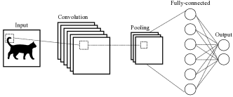
Figure 1: General structure of a CNN model.

II.2 Loss functions

The main mission one needs to accomplish when training the neural network is to minimize the difference between the output from the neural network and the true value as much as possible. The prediction is quantified by a metric called a loss function, which is optimized by adjusting the trainable parameters. For training our CNN and QCNN models of this study, several loss functions listed below are tested.

1) The cross-entropy loss is a measure of the classifier performance with an output probability between 0 and 1, and given by

$$\mathcal{L}_{\text{Cross-Entropy}}=-\frac{1}{N}\sum_{i=1}^{N}\left(y_{i}\log(\hat{y}_{i})+(1-y_{i})\log(1-\hat{y}_{i})\right)\,,$$ (1)

where $y_{i}$ is the true label of the $i$-th input, $\hat{y}_{i}$ is the corresponding label predicted by the model, and $N$ is the number of training data.

2) The Mean-Square-Error (MSE) considers binary labels $\pm 1$ and is given by

$$\mathcal{L}_{\text{MSE}}=\frac{1}{N}\sum_{i=1}^{N}(y_{i}-\hat{y}_{i})^{2}\,.$$ (2)

3) The Hinge loss also takes $\pm 1$ labels as inputs and defined as

$$\mathcal{L}_{\text{Hinge}}=\frac{1}{N}\sum_{i=1}^{N}\max(0,1-y_{i}\cdot\hat{y}_{i})\,.$$ (3)

Due to GPU’s limited capabilities, it is not possible to train the network with the whole dataset all at once when the dataset is too large. Therefore, the data is usually split into batches, where the number of samples that go through the network defines the batch size. When the network goes through the whole dataset, this is one epoch. Then this process is repeated until the loss function converges during optimization.

II.3 QCNNs

QCNN was a QNN model motivated by the success of CNNs [17]. The basic idea of QCNN is to utilize quantum operations to accomplish the convolution and pooling techniques and do the classification task using the outcome from the circuit. In the case of classical inputs (like images), we need to encode the data (image pixels) first as $\ket{\psi(\bm{x})}=U_{\text{enc}}(\bm{x})\ket{0}$, where $\bm{x}$ is classical data. Then the encoded state is processed via parametrized unitaries composed of convolutional and pooling blocks to have an output $\hat{y}$, given by

$$\hat{y}=\braket{\psi(\bm{x})}{U^{{\dagger}}_{\text{QCNN}}(\bm{\theta})Z_{N_{q}}U_{\text{QCNN}}(\bm{\theta})}{\psi(\bm{x})}\,,$$ (4)

where $N_{q}$ is the number of qubits. The overall structure for the QCNN with classical inputs is shown in Fig 2.

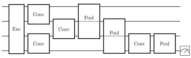
Figure 2: The structure of a full QCNN circuit. The first block (Enc.) corresponds to one of encodings given in Fig. 3, and the following blocks (conv. and pool.) are given in Fig. 4

II.3.1 Encodings

The encoding $V_{\text{enc}}$ can be done in several ways. We test four encoding schemes, namely: tensor product embedding (TPE) which in this case is also known as angle encoding, hardware efficient embedding (HEE), and Classically Hard Embedding (CHE). These three encodings are used to study the effects of encoding on trainability in [25]. The quantum circuit structure of the different encodings can be seen in Fig. 3, where TPE is shown in Fig. 3a, HEE in 3b, and CHE in 3c. The data inputs in these figures are represented by $x_{i}$, where $i\in\{0,1,2,3\}$. In this paper, we use one layer and two layers of HEE, denoted by HEE1 and HEE2, respectively. On the other hand, only one layer of CHE is used in this work. Since reference [25] showed that increasing the number of layers would cause trainability issues, we only focus on these encodings with the limited number of layers.

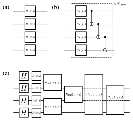
Figure 3: The four different encoding studied in this paper. TPE is represented in (a), HEE ($N_{\text{layer}}=1$ for HEE1 and $N_{\text{layer}}=2$ for HEE2) (b), and CHE (c).

II.3.2 Convolutional and Pooling circuits

After the encoding layer comes the convolutional layer. This layer consists of convolutional circuits connecting every pair of qubits to compensate for the task of a classical convolutional filter that scans over all the pixel values of an image. The convolutional circuit can be built in various ways. In this project, we test two unitary two-qubit circuits $SO(4)$ and $SU(4)$. The dimensionality of the trainable parameters $\bm{{\theta}}$ depends on these two-qubit unitaries. The circuit constructions for these unitaries are presented in Fig. 4a and 4b. The $SO(4)$ circuit corresponds to real transformation [26] and it contains 2 CNOTs and 12 single-qubit gates of which only 6 of them contain trainable parameters ($\bm{{\theta}}$). $SU(4)$ is more general and considered a universal two-qubit circuit spanning the whole Hilbert space. It consists of 3 CNOTs and 15 single-qubit gates all containing trainable parameters [26, 27]. Then, the convolutional circuit connects every pair of neighboring qubits until it forms a full convolutional layer.

After that comes the pooling layer to reduce the dimensionality of the system by half. The pooling circuit, shown in Fig. 4c, comprises a CNOT gate and 9 single-qubit gates all containing trainable parameters. The convolutional and pooling layers are repeated until the system has reached a sufficiently small size, one qubit in our case in which its output is measured with a PauliZ measurement, and the predicted output is then compared to the true label for the classification task as explained in Section II.2.

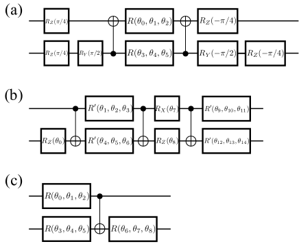
Figure 4: The quantum gates structure of $SO(4)$ (a) and $SU(4)$ (b) convolutional circuits, and pooling circuit (c), where $R(\alpha,\beta,\gamma)=R_{Z}(\gamma)R_{Y}(\beta)R_{Z}(\alpha)$ and $R^{\prime}(\alpha,\beta,\gamma)=R_{Z}(\gamma)R_{X}(\beta)R_{Z}(\alpha)$.

II.4 Dataset Preparation

As previously mentioned, the publicly available TopTagging dataset from the JetNet library [21] is used. The original given dataset consists of two types of jets: top jets and QCD jets. The data is given in the form of a group of particles in every jet, where every particle has its own four-momentum components. The general form of the four-momentum vector is given by

$$p^{\mu}=(E,p_{x},p_{y},p_{z})\,,$$ (5)

where its components are referred to as the particle’s features. The maximum number of particles provided in each jet is 200. The dataset is then preprocessed and transformed to form images. Then, we apply PCA to reduce dimensionality of the images. This reduction enables the use of a simple quantum circuit where each qubit takes a single pixel value from the image as an input.

II.4.1 Jet images

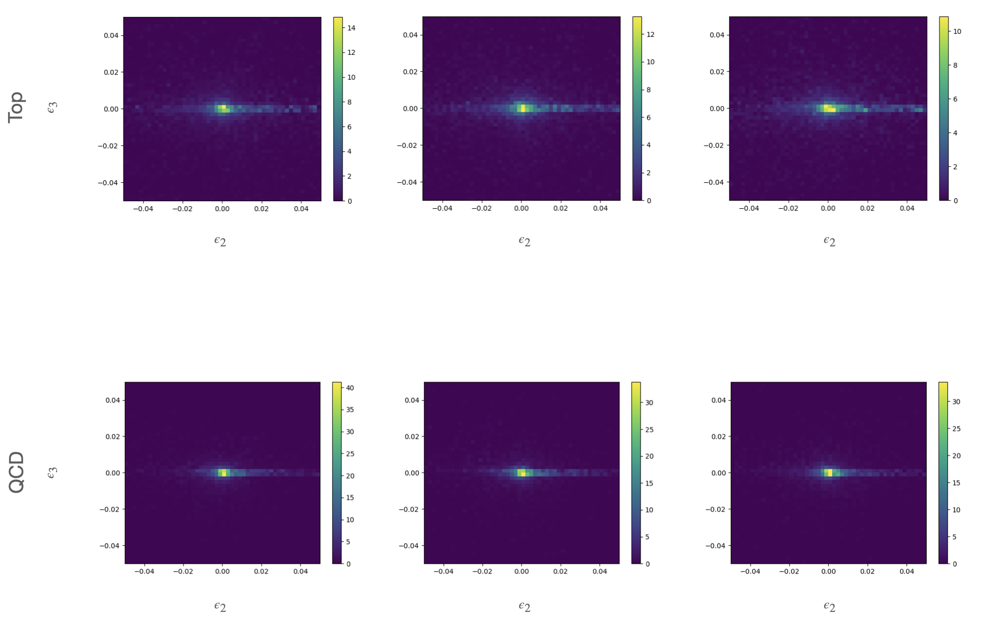
Figure 5: Examples of 50x50 jet images of top-quark (top) and QCD (bottom) jets from JetNet library.

Pre-processing and transformation techniques used to form the jet images are presented in references [15] and [28]. They have resulted in a highly reduced dependence for the jet images on the initial top quark momentum.

The idea of image processing is as follows. First, we re-scale the jet four-momentum such that its mass is $m_{B}$. Then, we apply a Lorentz boost such that the jet energy is $E_{B}$ in the new frame. Using $m_{B}$ and $E_{B}$ a fixed value for the Lorentz boost can be obtained from

$$\gamma_{B}=\frac{E_{B}}{m_{B}}\,.$$ (6)

In this project, $\gamma_{B}=10$ is chosen.

The transformation of the jet’s constituents is done using the Gram-Schmidt method. First, we choose the three constituents with the highest three-momentum ($\vec{\textbf{p}}_{1}$, $\vec{\textbf{p}}_{2}$, and $\vec{\textbf{p}}_{3}$) such that the total momentum of the jet is roughly

$$\vec{\textbf{P}}_{J}=\vec{\textbf{p}}_{1}+\vec{\textbf{p}}_{2}+\vec{\textbf{p}}_{3}.$$ (7)

Three vectors $\vec{\textbf{P}}_{J},\vec{\textbf{p}}_{1}$, and $\vec{\textbf{p}}_{2}$ can be considered as a set of linearly independent vectors, hence we can use them to construct the Gram-Schmidt orthonormal set of basis. We may choose one of the vectors in the set $\{\vec{\textbf{P}}_{J},\vec{\textbf{p}}_{1},\vec{\textbf{p}}_{2}\}$ to form the first Gram-Schmidt basis, and let it be $\vec{\textbf{P}}_{J}$ so that

$$\hat{\epsilon}_{1}=\frac{\vec{\textbf{P}}_{J}}{|\vec{\textbf{P}}_{J}|}\,.$$ (8)

The second basis has to be orthogonal to $\hat{\epsilon}_{1}$. Therefore, we can use the vector $\vec{\textbf{p}}_{1}$ and subtract from it the component that projects on $\hat{\epsilon}_{1}$ such that

$$\hat{\epsilon}_{2}=\frac{\vec{\textbf{p}}_{1}-(\vec{\textbf{p}}_{1}\cdot\hat{\epsilon}_{1})\hat{\epsilon}_{1}}{|\vec{\textbf{p}}_{1}-(\vec{\textbf{p}}_{1}\cdot\hat{\epsilon}_{1})\hat{\epsilon}_{1}|}\,.$$ (9)

Then the third basis that is orthogonal to $\hat{\epsilon}_{1}$ and $\hat{\epsilon}_{2}$ reads

$$\hat{\epsilon}_{3}=\frac{\vec{\textbf{p}}_{2}-(\vec{\textbf{p}}_{2}\cdot\hat{\epsilon}_{1})\hat{\epsilon}_{1}-(\vec{\textbf{p}}_{2}\cdot\hat{\epsilon}_{2})\hat{\epsilon}_{2}}{|\vec{\textbf{p}}_{2}-(\vec{\textbf{p}}_{2}\cdot\hat{\epsilon}_{1})\hat{\epsilon}_{1}-(\vec{\textbf{p}}_{2}\cdot\hat{\epsilon}_{2})\hat{\epsilon}_{2}|}\,.$$ (10)

The jet axis of the image is parallel to the first basis $\hat{\epsilon}_{1}$, hence the two-dimensional coordinates of the jet images $(X_{i},Y_{i})$ are related to the jet constituent $i$ having the four-momentum $p^{\mu}_{i}=(p^{0}_{i},\vec{p}_{i})$ through the formulae

$$X_{i}=\frac{\vec{p}_{i}\cdot\hat{\epsilon}_{2}}{p^{0}_{i}}\,,\quad Y_{i}=\frac{\vec{p}_{i}\cdot\hat{\epsilon}_{3}}{p^{0}_{i}}\,.$$ (11)

If we neglect the mass of the constituent, and as a consequence of the Gram-Schmidt unitary transformation that preserves the magnitudes of the transformed vectors, we would have

$$|\vec{p}_{i}|^{2}=(p^{0}_{i})^{2}=(\vec{p}_{i}\cdot\hat{\epsilon}_{1})^{2}+(\vec{p}_{i}\cdot\hat{\epsilon}_{2})^{2}+(\vec{p}_{i}\cdot\hat{\epsilon}_{3})^{2}.$$ (12)

This means that the components $X_{i}$ and $Y_{i}$ can only be in the range of $[-1,1]$. These components then form the coordinates of the two-dimensional histogram corresponding to the jet image. The histogram is filled with the weight

$$\omega_{i}=\frac{p^{0}_{i}}{E_{B}},$$ (13)

representing the fraction of energy for the constituent $i$. The goal of the Gram-Schmidt transformation is to make the jet images look similar regardless of the difference in the initial top-quark boost. This helps the machine learning networks to learn the features from images more easily. Examples of top-quark and QCD jets summed over 10,000 images are shown in Fig. 5. We can already notice the similarity between the top and QCD jet images which increases the complexity of the analysis. The main differences one could notice are the slightly larger spread of the top jet compared to the QCD jet and the values of the energy fractions given in the color bars beside each histogram. We use 2,000 of these images, resized to $28\times 28$ pixels, for our training task in QCNN and CNN. The dataset is split into 80$\%$ for training and 20$\%$ for testing.

II.4.2 PCA

Principal Component Analysis (PCA) (see e.g. [29]) is a method that is commonly used to find patterns while reducing the dimensionality of data. It mainly captures correlation in data and transforms it into a new set of variables that better describes the patterns. These variables are called the principal components. In this project, PCA is used to reduce the dimensionality of the jet images from $28\times 28$ to $2\times 2$, so that we end up with only 4 pixels that are the inputs of our QCNN and CNN models.

III Results

The results presented here are based on a qualitative level comparison. We obtain accuracy and loss results for different setups using the default.qubit simulator from PennyLane for quantum computing calculations, and the TensorFlow library for CNNs. Results are obtained separately for $SO(4)$ and $SU(4)$ quantum circuits, considering the three loss functions, Hinge, MSE, and Cross-entropy. For each loss function, in the first step, we change the encodings (TPE, HEE1, HEE2, and CHE) while keeping the batch-size fixed to 32. Then we choose the opposite, namely, we fix the encoding to HEE1 and change the batch-sizes (16, 32, 64, and 128).

To ensure a fair comparison between QCNNs and CNNs, we aim to make their overall setups as similar as possible. The number of trainable parameters plays a significant role in achieving good classical results. Therefore, for an $SO(4)$ QCNN with 30 parameters, the corresponding number of CNN parameters is 33. Similarly, for an $SU(4)$ QCNN with 48 parameters, the corresponding number for CNN is 51. For every run, we initialize a random set of parameters that are optimized after each epoch with a learning rate of $0.001$.

On top of the loss values, additional metric is used to measure the accuracy, which is given by the total number of correct classifications over the total number of all classifications, that is

$$\text{(accuracy)}:=\frac{\text{(correct classifications)}}{\text{(the number of total samples)}}\,.$$ (14)

III.1 Dependence on Encodings

Circuit	Loss function	Encoding	QCNN Acc ($\%$)	CNN Acc ($\%$)
SO(4)	Hinge	TPE	98.60 $\pm$ 0.20	94.76 ± 2.17
		HEE1	99.22 $\pm$ 0.11
		HEE2	96.49 ± 0.39
		CHE	94.47 ± 0.28
	MSE	TPE	99.37 ± 0.11	90.81 ± 2.78
		HEE1	99.84 ± 0.06
		HEE2	97.99 ± 0.28
		CHE	96.92 ± 0.18
	Cross-entropy	TPE	98.82 ± 0.17	94.77 ± 2.17
		HEE1	99.48 ± 0.09
		HEE2	97.16 ± 0.34
		CHE	95.71 ± 0.22
SU(4)	Hinge	TPE	99.36 ± 0.13	99.88 ± 0.05
		HEE1	99.34 ± 0.10
		HEE2	98.30 ± 0.18
		CHE	95.58 ± 0.34
	MSE	TPE	99.93 ± 0.03	99.95 ± 0.02
		HEE1	99.90 ± 0.05
		HEE2	99.28 ± 0.11
		CHE	97.97 ± 0.12
	Cross-entropy	TPE	99.58 ± 0.08	99.92 ± 0.03
		HEE1	99.62 ± 0.05
		HEE2	98.62 ± 0.16
		CHE	96.70 ± 0.18

Table 1: Test accuracy for tensor product embedding (TPE), hardware efficient embedding with one later (HEE1) and two layers (HEE2), and the classically hard embedding (CHE) results averaged over 50 runs for $SO(4)$ with 30 parameters and CNN results with 33 parameters, and $SU(4)$ with 48 parameters and the comparable CNN with 51 parameters. The batch-size is fixed to 32.

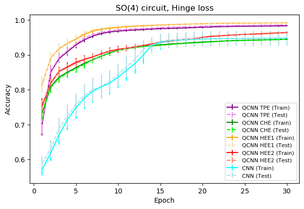
(a)

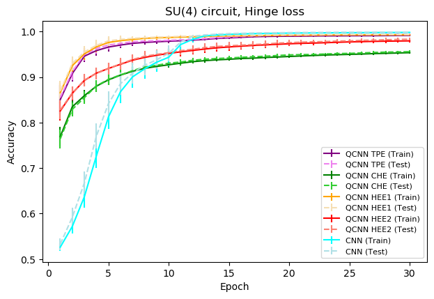
(b)

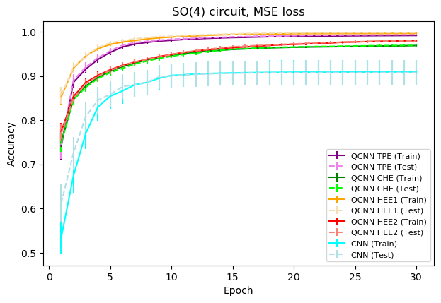
(c)

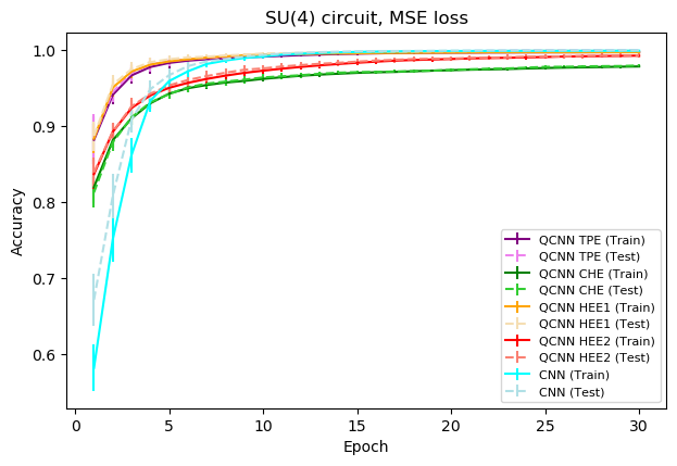
(d)

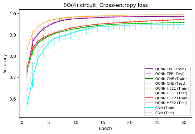
(e)

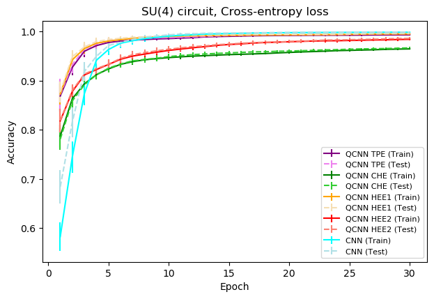
(f)

Figure 6: $SO(4)$ and $SU(4)$ QCNN accuracy encoding results compared to CNN for Hinge (a) and (b), MSE (c) and (d), and Cross-entropy (e) and (f).

Accuracy results after $30$ epochs averaged over $50$ runs for QCNN with $SO(4)$ and $SU(4)$ with varying (quantum) encoding types compared to CNN for the three loss functions are presented in Table 1. Here, the batch-size is fixed to 32. We can notice that accuracy results for QCNN are better than those of CNN when we use $SO(4)$ along with Hinge (except for CHE encoding), MSE, or cross-entropy. The performance of QCNN for $SU(4)$ setups is similar or worse. We can also observe the relatively large error for CNN results at the low parameter regime. For QCNN setups, first with relatively high accuracy, HEE1 encoding (values given in bold in Table 1), and then TPE showed better results compared to HEE2 or CHE. This could be possibly understood from dataset induced barren plateau investigated in [25]. In other words, the HEE2 and CHE encoding would be too complex specifically for this task, which induces trainability issues (barren plateau). However, we have to study performance by increasing the number of qubits to make this connection more concretely, which we leave for the future direction.

The accuracy curves corresponding to these settings are also summarized in Fig. 6 for $SO(4)$ and $SU(4)$ compared to CNN with Hinge (Fig. 6(a) and 6(b)), MSE (Fig. 6(c) and 6(d)), and Cross-entropy (Fig. 6(e) and 6(f)) loss functions. We can notice the faster convergence at early epochs for all setups of QCNN for both $SO(4)$ and $SU(4)$ compared to CNN.

III.2 Dependence on Batch-sizes

Circuit	Loss function	Batch-size	QCNN Acc ($\%$)	CNN Acc ($\%$)
SO(4)	Hinge	16	99.56 ± 0.05	87.79 ± 3.09
		32	99.48 ± 0.07	90.84 ± 2.78
		64	99.05 ± 0.18	89.46 ± 2.87
		128	96.48 ± 0.62	77.86 ± 3.41
	MSE	16	99.90 ± 0.04	93.87 ± 2.35
		32	99.86 ± 0.05	89.76 ± 2.89
		64	99.70 ± 0.08	93.72 ± 2.35
		128	98.23 ± 0.25	91.50 ± 2.38
	Cross-entropy	16	99.71 ± 0.05	91.88 ± 2.66
		32	99.55 ± 0.06	91.78 ± 2.65
		64	99.28 ± 0.17	93.59 ± 2.34
		128	97.53 ± 0.30	98.23 ± 1.03
SU(4)	Hinge	16	99.43 ± 0.08	99.97 ± 0.02
		32	99.47 ± 0.07	99.95 ± 0.03
		64	99.14 ± 0.12	97.87 ± 1.42
		128	98.52 ± 0.22	94.81 ± 1.82
	MSE	16	99.98 ± 0.01	100.00 ± 0.00
		32	99.95 ± 0.04	99.96 ± 0.02
		64	99.84 ± 0.04	99.92 ± 0.03
		128	99.43 ± 0.13	99.36 ± 0.22
	Cross-entropy	16	99.54 ± 0.06	100.00 ± 0.00
		32	99.60 ± 0.07	99.995 ± 0.005
		64	99.40 ± 0.10	98.76 ± 1.01
		128	98.93 ± 0.17	98.77 ± 0.41

Table 2: Test accuracy batch-sizes results averaged over 50 runs for $SO(4)$ with 30 parameters and their corresponding CNN with 33 parameters, and $SU(4)$ with 48 parameters and the comparable CNN with 51 parameters. Encoding is fixed to HEE1.

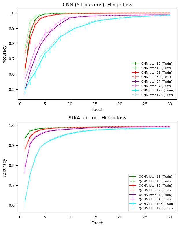
Figure 7: Accuracy results of the different batch-sizes in CNN (top) and $SU(4)$ QCNN (bottom) for Hinge loss.

After fixing the encoding to HEE1 which shows the best performance for $32$ batch-size, we varied the batch size to four different sizes. The results averaged over $50$ runs are displayed in Table 2. Again we observe a tendency for QCNN to have a better performance for most of the batch-sizes in $SO(4)$ compared to CNN, and results are comparable for $SU(4)$ and CNN. However, what is clearly noticeable in most of the cases, is that as the batch size increases, the accuracy tends to decrease. This observation is also depicted in Fig. 7 for $SU(4)$ and the corresponding CNN model with $51$ parameters for Hinge loss as an example. We also observe that a batch size of $16$ has faster convergence compared to the other batch sizes, while a batch size of $128$ exhibits the slowest convergence. Batch sizes of 16 and 32 demonstrate similar performance (values shown in bold in Table 2), which is superior to both 64 and 128. It is essential to note that slower or faster convergence does not necessarily equate to slower or faster training times, since the time it takes to train each epoch is different from quantum to classical.

IV Conclusion and outlook

In this paper, we utilized two QCNN architectures one with $SO(4)$ convolutional circuit and the other built with an $SU(4)$ convolutional circuit. We varied the setups of each architecture to test different loss functions, encodings, and batch-sizes. We compared each setup with a corresponding CNN model. From the preliminary results we got for our quantum and classical models, we found that the QCNN, in the absence of noise, performs better than the corresponding CNN model for a specific choice of data encoding, batch-size, loss function, and convolutional block, at least for this task along with PCA, but do not otherwise. However, we need to emphasize that the system we studied here was relatively simple, both in QCNN and CNN, therefore, it was possible to train the classical model with a very small number of parameters, whereas the usual case of training CNN models is to use a high number of parameters that may reach up to millions. Besides, we only performed the noiseless simulation and the effects from noise would spoil the QCNN performance unless we can tame them.

Aiming to noisy hardware implementation, it would be better to reduce the complexity of a circuit as much as possible. We could try the following two methods for this purpose. The first one is dimensional expressivity analysis (DEA) proposed in [30]. DEA helps detect redundant parameters and potentially optimize the circuit which may result in reduced training time, less noise from quantum gates, and better suitability for real quantum hardware. Current DEA is done after setting up all circuit elements including embedding gates. Because embedding circuits in QML can change depending on different input images, we have to modify DEA to check for the redundant parameters for every single input image. If this is achieved successfully, it might result in a dynamic QNN (DQNN) which could be more flexible and adaptive to the type of data used. The second one is the equivariant QNN (EQNN) [31] which mainly relies on the symmetry found in data. EQNN methods allow us to construct QNNs that automatically satisfy the desired symmetry constraints. Since our dataset can also have rotational symmetry thus potentially, we can apply these techniques.

On top of reducing the circuit complexity, an important ingredient for the realization on noisy devices is an error mitigation method, such as zero noise extrapolation (ZNE) [32, 33, 34], probabilistic error cancellation [33, 35], and Twirled Readout Error eXtinction (TREX) [36].

Ultimately, it would be important to study the scaling of performance and resources with respect to the complexity of the dataset and/or the number of qubits. It would be interesting if we could combine the techniques listed above to see the scaling on the actual hardware.

References

- Schuld et al. [2014] M. Schuld, I. Sinayskiy, and F. Petruccione, An introduction to quantum machine learning, Contemporary Physics 56, 172–185 (2014).
- Biamonte et al. [2017] J. Biamonte, P. Wittek, N. Pancotti, P. Rebentrost, N. Wiebe, and S. Lloyd, Quantum machine learning, Nature 549, 195–202 (2017).
- Mangini et al. [2021] S. Mangini, F. Tacchino, D. Gerace, D. Bajoni, and C. Macchiavello, Quantum computing models for artificial neural networks, Europhysics Letters 134, 10002 (2021).
- Cerezo et al. [2022] M. Cerezo, G. Verdon, H.-Y. Huang, L. Cincio, and P. Coles, Challenges and opportunities in quantum machine learning, Nature Computational Science 2 (2022).
- Mitarai et al. [2018] K. Mitarai, M. Negoro, M. Kitagawa, and K. Fujii, Quantum circuit learning, Physical Review A 98, 10.1103/physreva.98.032309 (2018).
- Farhi and Neven [2018] E. Farhi and H. Neven, Classification with quantum neural networks on near term processors, arXiv preprint arXiv:1802.06002 (2018), arXiv:1802.06002 .
- Benedetti et al. [2019] M. Benedetti, E. Lloyd, S. Sack, and M. Fiorentini, Parameterized quantum circuits as machine learning models, Quantum Sci. Technol. 4, 043001 (2019), arXiv:1906.07682 [quant-ph] .
- Schuld et al. [2020] M. Schuld, A. Bocharov, K. M. Svore, and N. Wiebe, Circuit-centric quantum classifiers, Phys. Rev. A 101, 032308 (2020).
- Guan et al. [2021] W. Guan, G. Perdue, A. Pesah, M. Schuld, K. Terashi, S. Vallecorsa, and J.-R. Vlimant, Quantum Machine Learning in High Energy Physics, Mach. Learn. Sci. Tech. 2, 011003 (2021), arXiv:2005.08582 [quant-ph] .
- Felser et al. [2021] T. Felser, M. Trenti, L. Sestini, A. Gianelle, D. Zuliani, D. Lucchesi, and S. Montangero, Quantum-inspired machine learning on high-energy physics data (2021), arXiv:2004.13747 [stat.ML] .
- Araz and Spannowsky [2021] J. Y. Araz and M. Spannowsky, Quantum-inspired event reconstruction with tensor networks: Matrix product states, Journal of High Energy Physics 2021, 10.1007/jhep08(2021)112 (2021).
- Araz and Spannowsky [2022] J. Y. Araz and M. Spannowsky, Classical versus quantum: Comparing tensor-network-based quantum circuits on large hadron collider data, Physical Review A 106, 10.1103/physreva.106.062423 (2022).
- Gianelle et al. [2022] A. Gianelle, P. Koppenburg, D. Lucchesi, D. Nicotra, E. Rodrigues, L. Sestini, J. de Vries, and D. Zuliani, Quantum machine learning for b-jet charge identification, Journal of High Energy Physics 2022, 10.1007/jhep08(2022)014 (2022).
- Belis et al. [2024] V. Belis, P. Odagiu, and T. K. Aarrestad, Machine learning for anomaly detection in particle physics, Reviews in Physics 12, 100091 (2024).
- Bhattacharya et al. [2022] S. Bhattacharya, M. Guchait, and A. H. Vijay, Boosted top quark tagging and polarization measurement using machine learning, Phys. Rev. D 105, 042005 (2022).
- Butter et al. [2019] A. Butter et al., The Machine Learning landscape of top taggers, SciPost Phys. 7, 014 (2019), arXiv:1902.09914 [hep-ph] .
- Cong et al. [2019] I. Cong, S. Choi, and M. D. Lukin, Quantum convolutional neural networks, Nature Physics (2019) https://doi.org/10.1038/s41567-019-0648-8 (2019).
- Pesah et al. [2021] A. Pesah, M. Cerezo, S. Wang, T. Volkoff, A. T. Sornborger, and P. J. Coles, Absence of barren plateaus in quantum convolutional neural networks, Phys. Rev. X 11, 041011 (2021) https://doi.org/10.1103/PhysRevX.11.041011 (2021).
- Hur et al. [2021] T. Hur, L. Kim, and D. K. Park, Quantum convolutional neural network for classical data classification, Quantum Machine Intelligence 4, 3 (2022) https://doi.org/10.1007/s42484-021-00061-x (2021).
- Chen et al. [2022] S. Y.-C. Chen, T.-C. Wei, C. Zhang, H. Yu, and S. Yoo, Quantum convolutional neural networks for high energy physics data analysis, Phys. Rev. Res. 4, 013231 (2022), arXiv:2012.12177 [cs.LG] .
- Kansal et al. [2023] R. Kansal, C. Pareja, Z. Hao, and J. Duarte, JetNet: A Python package for accessing open datasets and benchmarking machine learning methods in high energy physics, Journal of Open Source Software 8, 5789 (2023).
- Bergholm et al. [2018] V. Bergholm et al., PennyLane: Automatic differentiation of hybrid quantum-classical computations, (2018), arXiv:1811.04968 [quant-ph] .
- Abadi et al. [2015] M. Abadi, A. Agarwal, P. Barham, E. Brevdo, Z. Chen, C. Citro, G. S. Corrado, A. Davis, J. Dean, M. Devin, S. Ghemawat, I. Goodfellow, A. Harp, G. Irving, M. Isard, Y. Jia, R. Jozefowicz, L. Kaiser, M. Kudlur, J. Levenberg, D. Mané, R. Monga, S. Moore, D. Murray, C. Olah, M. Schuster, J. Shlens, B. Steiner, I. Sutskever, K. Talwar, P. Tucker, V. Vanhoucke, V. Vasudevan, F. Viégas, O. Vinyals, P. Warden, M. Wattenberg, M. Wicke, Y. Yu, and X. Zheng, TensorFlow: Large-scale machine learning on heterogeneous systems (2015), software available from tensorflow.org.
- O’Shea and Nash [2015] K. O’Shea and R. Nash, An Introduction to Convolutional Neural Networks, arXiv e-prints , arXiv:1511.08458 (2015), arXiv:1511.08458 [cs.NE] .
- Thanasilp et al. [2021] S. Thanasilp, S. Wang, N. A. Nghiem, P. J. Coles, and M. Cerezo, Subtleties in the trainability of quantum machine learning models, arXiv e-prints , arXiv:2110.14753 (2021), arXiv:2110.14753 [quant-ph] .
- Vatan and Williams [2004] F. Vatan and C. Williams, Optimal quantum circuits for general two-qubit gates, Phys. Rev. A 69, 032315 (2004) https://doi.org/10.1103/PhysRevA.69.032315 (2004).
- Shende et al. [2004] V. V. Shende, I. L. Markov, and S. S. Bullock, Minimal universal two-qubit controlled-not-based circuits, Phys. Rev. A 69, 062321 (2004).
- Roy and Vijay [2019] T. S. Roy and A. H. Vijay, A robust anomaly finder based on autoencoders, arXiv e-prints , arXiv:1903.02032 (2019), arXiv:1903.02032 [hep-ph] .
- Jolliffe and Cadima [2016] I. T. Jolliffe and J. Cadima, Principal component analysis: a review and recent developments, Philosophical transactions of the royal society A: Mathematical, Physical and Engineering Sciences 374, 20150202 (2016).
- Funcke et al. [2021] L. Funcke, T. Hartung, K. Jansen, S. Kühn, and P. Stornati, Dimensional expressivity analysis of parametric quantum circuits, Quantum 5, 422 (2021) https://doi.org/10.22331/q-2021-03-29-422 (2021).
- Forestano et al. [2024] R. T. Forestano, M. Comajoan Cara, G. R. Dahale, Z. Dong, S. Gleyzer, D. Justice, K. Kong, T. Magorsch, K. T. Matchev, K. Matcheva, and E. B. Unlu, A comparison between invariant and equivariant classical and quantum graph neural networks, Axioms 13, 160 (2024).
- Li and Benjamin [2017] Y. Li and S. C. Benjamin, Efficient variational quantum simulator incorporating active error minimization, Phys. Rev. X 7, 021050 (2017).
- Temme et al. [2017] K. Temme, S. Bravyi, and J. M. Gambetta, Error mitigation for short-depth quantum circuits, Phys. Rev. Lett. 119, 180509 (2017).
- Majumdar et al. [2023] R. Majumdar, P. Rivero, F. Metz, A. Hasan, and D. S. Wang, Best practices for quantum error mitigation with digital zero-noise extrapolation, (2023), arXiv:2307.05203 [quant-ph] .
- van den Berg et al. [2023] E. van den Berg, Z. K. Minev, A. Kandala, and K. Temme, Probabilistic error cancellation with sparse Pauli-Lindblad models on noisy quantum processors, Nature Physics 19, 1116 (2023), arXiv:2201.09866 [quant-ph] .
- van den Berg et al. [2022] E. van den Berg, Z. K. Minev, and K. Temme, Model-free readout-error mitigation for quantum expectation values, Phys. Rev. A 105, 032620 (2022).
- Kingma and Ba [2014] D. P. Kingma and J. Ba, Adam: A Method for Stochastic Optimization, arXiv e-prints , arXiv:1412.6980 (2014), arXiv:1412.6980 [cs.LG] .