Can Large Language Models Improve the Adversarial Robustness of Graph Neural Networks?

Abstract.

Graph neural networks (GNNs) are vulnerable to adversarial perturbations, especially for topology attacks, and many methods that improve the robustness of GNNs have received considerable attention. Recently, we have witnessed the significant success of large language models (LLMs), leading many to explore the great potential of LLMs on GNNs. However, they mainly focus on improving the performance of GNNs by utilizing LLMs to enhance the node features. Therefore, we ask: Will the robustness of GNNs also be enhanced with the powerful understanding and inference capabilities of LLMs? By presenting the empirical results, we find that despite that LLMs can improve the robustness of GNNs, there is still an average decrease of 23.1% in accuracy, implying that the GNNs remain extremely vulnerable against topology attack. Therefore, another question is how to extend the capabilities of LLMs on graph adversarial robustness. In this paper, we propose an LLM-based robust graph structure inference framework, LLM4RGNN, which distills the inference capabilities of GPT-4 into a local LLM for identifying malicious edges and an LM-based edge predictor for finding missing important edges, so as to recover a robust graph structure. Extensive experiments demonstrate that LLM4RGNN consistently improves the robustness across various GNNs. Even in some cases where the perturbation ratio increases to 40%, the accuracy of GNNs is still better than that on the clean graph.

1   Introduction

Graph neural networks (GNNs), as representative graph machine learning methods, effectively utilize their message-passing mechanism to extract useful information and learn high-quality representations from graph data (kipf2016semi, ; velivckovic2017graph, ; wu2020comprehensive, ). Despite great success, a host of studies have shown that GNNs are vulnerable to adversarial attacks (sun2022adversarial, ; li2022revisiting, ; mujkanovic2022defenses, ; waniek2018hiding, ; jin2021adversarial, ), especially for topology attacks (zugner_adversarial_2019, ; zugner2018adversarial, ; xu2019topology, ), where slightly perturbing the graph structure can lead to a dramatic decrease in the performance. Such vulnerability poses significant challenges for applying GNNs to real-world applications, especially in security-critical scenarios such as finance networks (wang2021review, ) or medical networks (mao2019medgcn, ).

Threatened by adversarial attacks, several attempts have been made to build robust GNNs, which can be mainly divided into model-centric and data-centric defenses (zheng2021grb, ). From the model-centric perspective, defenders can improve robustness through model enhancement, either by robust training schemes (li2023boosting, ; gosch2024adversarial, ) or new model architectures (zhu2019robust, ; jin2021node, ; zhao2024adversarial, ). In contrast, data-centric defenses typically focus on flexible data processing to improve the robustness of GNNs. Treating the attacked topology as noisy, defenders primarily purify graph structures by calculating various similarities between node embeddings (wu2019adversarial, ; jin2020graph, ; zhang2020gnnguard, ; li2022reliable, ; entezari2020all, ). The above methods have received considerable attention in enhancing the robustness of GNNs.

Recently, large language models (LLMs), such as GPT-4 (achiam2023gpt, ), have demonstrated expressive capabilities in understanding and inferring complex texts, revolutionizing the fields of natural language processing (zhao2023survey, ), computer vision (yin2023survey, ) and graph (liu2023towards, ). The performance of GNNs can be greatly improved by utilizing LLMs to enhance the node features (he2023harnessing, ; liu2023one, ; chen2024exploring, ). However, one question remains largely unknown: Considering the powerful understanding and inference capabilities of LLMs, will LLMs enhance or weaken the adversarial robustness of GNNs to a certain extent? Answering this question not only helps explore the potential capabilities of LLMs on graphs, but also provides a new perspective for the adversarial robustness problem on graphs.

Here, we empirically investigate the robustness of GNNs combining six LLMs/LMs (language models), namely OFA-Llama2-7B (liu2023one, ), OFA-SBert (liu2023one, ), TAPE (he2023harnessing, ), GCN-Llama-7B (chen2024exploring, ), GCN-e5-large (chen2024exploring, ), and GCN-SBert (chen2024exploring, ), against Mettack (zugner_adversarial_2019, ) with a 20% perturbation rate on Cora (mccallum2000automating, ) and PubMed (sen2008collective, ) datasets. As shown in Figure 1, the results clearly show that these models suffer from a maximum accuracy decrease of 37.9% and an average of 23.1%, while vanilla GCN (kipf2016semi, ) experiences a maximum accuracy decrease of 39.1% and an average of 35.5%. It demonstrates that these models remain extremely vulnerable to topology perturbations (more details refer to Section 3). Consequently, another question naturally arises: How to extend the capabilities of LLMs to improve graph adversarial robustness? This problem is non-trivial because graph adversarial attacks typically perturb the graph structures, while the capabilities of LLMs usually focus on text processing. Considering that graph structures involve complex interactions among a large number of nodes, how to efficiently explore the inference capabilities of LLMs on perturbed structures is a significant challenge.

In this paper, we propose an LLM-based robust graph structure inference framework, called LLM4RGNN, which efficiently utilizes LLMs to purify the perturbed structure, improving the adversarial robustness. Specifically, based on an open-source and clean graph structure, we design a prompt template that enables GPT-4 (achiam2023gpt, ) to infer how malicious an edge is and provide analysis, to construct an instruction dataset. This dataset is used to fine-tune a local LLM (e.g., Mistral-7B (jiang2023mistral, ) or Llama3-8B (touvron2023llama, )), so that the inference capability of GPT-4 can be distilled into the local LLM. When given a new attacked graph structure, we first utilize the local LLM to identify malicious edges. By treating identification results as edge labels, we further distill the inference capability from the local LLM to an LM-based edge predictor, to find missing important edges. Finally, purifying the graph structure by removing malicious edges and adding important edges, makes GNNs more robust.

Our contributions can be summarized four-fold:

• To the best of our knowledge, we are the first to explore the potential of LLMs on the graph adversarial robustness. Moreover, we verify the vulnerability of GNNs even with the powerful understanding and inference capabilities of LLMs.

• We propose a novel LLM-based robust graph structure inference framework, called LLM4RGNN, which efficiently utilizes LLMs to make GNNs more robust. Additionally, LLM4RGNN is a general framework, suitable for different LLMs and GNNs.

• Extensive experiments demonstrate that LLM4RGNN consistently improves the robustness of various GNNs against topology attacks. Even in some cases where the perturbation ratio increases to 40%, the accuracy of GNNs with LLM4RGNN is still better than that on the clean graph.

• We utilize GPT-4 to construct an instruction dataset, including GPT-4’s maliciousness assessments and analyses of 26,000 edges. This dataset will be publicly released, which can be used to tune any other LLMs so that they can have the robust graph structure inference capability as GPT-4.

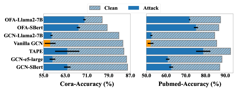
Figure 1. The accuracy of different GNNs combining LLMs/LMs against Mettack with a 20% perturbation rate.

2   Preliminaries

2.1. Text-attributed Graphs (TAGs)

Here, a Text-attributed graph (TAG), defined as $\mathcal{G}=(\mathcal{V},\mathcal{E},\mathcal{S})$, is a graph with node-level textual information, where $\mathcal{V}=\{v_{1},\ldots,v_{\left|\mathcal{V}\right|}\}$, $\mathcal{E}=\{e_{1},\ldots,e_{\left|\mathcal{E}\right|}\}$ and $\mathcal{S}=\{s_{1},\ldots,s_{\left|\mathcal{V}\right|}\}$ are the node set, edge set, and text set, respectively. The adjacency matrix of the graph $\mathcal{G}$ is denoted as $\mathbf{A}\in\mathbb{R}^{\left|\mathcal{V}\right|\times\left|\mathcal{V}\right|}$, where $\mathbf{A}_{ij}=1$ if nodes $v_{i}$ and $v_{j}$ are connected, otherwise $\mathbf{A}_{ij}=0$. In this work, we focus on the node classification task on TAGs. Specifically, each node $v_{i}$ corresponds to a label $y_{i}$ that indicates which category the node $v_{i}$ belongs to. Usually, we encode the text set $\mathcal{S}$ as the node feature matrix $\mathbf{X}=\{\mathbf{x}_{1},\dots,\mathbf{x}_{\left|\mathcal{V}\right|}\}$ via some embedding techniques (mikolov2013distributed, ; harris1954distributional, ; chen2024exploring, ) to train GNNs, where $\mathbf{x}_{i}\in\mathbb{R}^{d}$. Given some labeled nodes $\mathcal{V}_{L}\subset\mathcal{V}$, the goal is training a GNN $f(\mathbf{A},\mathbf{X})$ to predict the labels of the remaining unlabeled nodes $\mathcal{V}_{U}=\mathcal{V}\setminus\mathcal{V}_{L}$.

Figure 2. The framework of LLM4RGNN, which involves three main parts: (a) instruction tuning a local LLM, which distills the inference capability from GPT-4 into a local LLM for identifying malicious edges; (b) training an LM-based edge predictor, which further distills the inference capability from the local LLM into LM-based edge predictor for finding missing important edges; (c) purifying the graph structure by removing malicious edges and adding important edges, making GNNs more robust.

2.2. Graph Adversarial Robustness

This paper primarily focuses on stronger poisoning attacks, which can lead to an extremely low model performance by directly modifying the training data (zhu2019robust, ; zugner2018adversarial, ). The formal definition of adversarial robustness against poisoning attacks is as follows:

(1) $$\max_{\delta\in\Delta}\min_{\theta}\mathcal{L}(f_{\theta}(\mathcal{G}+\delta),\mathbf{y}_{\mathcal{T}}),$$

where $\delta$ represents a perturbation to the graph $\mathcal{G}$, which may include perturbations to node features, inserting or deleting of edges, etc., $\Delta$ represents all permitted and effective perturbations. $\mathbf{y}_{\mathcal{T}}$ is the node labels of the target set ${\mathcal{T}}$. $\mathcal{L}$ denotes the training loss of GNNs, and $\theta$ is the model parameters of $f$. Equation 1 indicates that under the worst-case perturbation $\delta$, the adversarial robustness of model $f$ is represented by its performance on the target set $\mathcal{T}$. A smaller loss value suggests stronger adversarial robustness, i.e., better model performance. In this paper, we primarily focus on the robustness under two topology attacks: 1) Targeted attacks (zugner2018adversarial, ), where attackers aim to mislead the model’s prediction on specific nodes $v$ by manipulating the adjacent edges of $v$, thus $\mathcal{T}={v}$. 2) Non-targeted attacks (zugner_adversarial_2019, ; waniek2018hiding, ), where attackers aim to degrade the overall performance of GNNs but do not care which node is being targeted, thus $\mathcal{T}=V_{\text{test}}$, where $V_{\text{test}}$ denotes the test set.

3   The Adversarial Robustness of GNNs Combining LLMs/LMs

In this paper, we empirically investigate whether LLMs enhance or weaken the adversarial robustness of GNNs to a certain extent. Specifically, for the Cora (mccallum2000automating, ) and PubMed (sen2008collective, ) datasets, based on non-contextualized embeddings encoded by BoW (harris1954distributional, ) or TF-IDF (robertson2004understanding, ), we employ Mettack (zugner_adversarial_2019, ) with a 20% perturbation rate to generate attack topology. We compare seven representative baselines: TAPE (he2023harnessing, ) utilizes LLMs to generate extra semantic knowledge relevant to the nodes. OFA (liu2023one, ) employs LLMs to unify different graph data and tasks, where OFA-SBert utilizes Sentence Bert (reimers2019sentence, ) to encode the text of nodes, training and testing the GNNs on each dataset independently. OFA-Llama2-7B involves training a single GNN across the Cora, Pubmed, and OGBN-Arxiv (hu2020open, ) datasets. Following the work (chen2024exploring, ), GCN-Llama2-7B, GCN-e5-large, and GCN-SBert represent the use of Llama2-7B, e5-large, and Sentence Bert as nodes’ text encoders, respectively. The vanilla GCN directly utilizes non-contextual embeddings. By reporting the node classification accuracy on $V_{\text{test}}$ to evaluate the robustness of models against the Mettack. The implementation details of baselines refer to Appendix B. The result is depicted in Figure 1. We observe that under the influence of Mettack, GNNs combining LLMs/LMs suffer from a maximum accuracy decrease of 37.9% and an average decrease of 23.1%, while vanilla GCN (kipf2016semi, ) suffers from a maximum accuracy decrease of 39.1% and an average accuracy decrease of 35.5%. The results demonstrate that GNNs combining LLMs/LMs remain extremely vulnerable against topology perturbations.

4   LLM4RGNN: The Proposed Framework

In this section, we propose a novel LLM-based robust graph structure inference framework, LLM4RGNN. As shown in Figure 2, LLM4RGNN distills the inference capabilities of GPT-4 into a local LLM for identifying malicious edges and an edge predictor for finding missing important edges, so as to recover a robust graph structure, making various GNNs more robust.

4.1. Instruction Tuning a Local LLM

Given an attacked graph structure, one straightforward method is to query powerful GPT-4 to identify malicious edges on the graph. However, this method is extremely expensive, because there are ${\left|\mathcal{V}\right|}^{2}$ different perturbation edges on a graph. For example, for the PubMed (sen2008collective, ) dataset with 19,717 nodes, the cost is approximately $9.72 million. Thus, we hope to distill the inference capability of GPT-4 into a local LLM, to identify malicious edges. To this end, instruction tuning based on GPT-4 is a popular fine-tuning technique (xu2024survey, ; chen2023label, ), which utilizes GPT-4 to construct an instruction dataset, and then further trains a local LLM in a supervised fashion. The instruction dataset generally consists of instance (instruction, input, output), where instruction denotes the human instruction (a task definition in natural language) for LLMs, input is used as supplementary content for the instruction, and output denotes the desired output that follows the instruction. Therefore, the key is how to construct an effective instruction dataset for fine-tuning an LLM to identify the malicious edges.

In the tuning local LLMs phase of Figure 2 (a), based on an open-source and clean graph structure $\mathbf{A}$ (TAPE-Arxiv23 (he2023harnessing, )), we utilize the existing attacks (Mettack (zugner_adversarial_2019, ), Nettack (zugner2018adversarial, ), and Minmax (xu2019topology, )) to generate the perturbed graph structure $\mathbf{A}^{\prime}$, thus we have the modification matrix $\mathbf{S}$ as follows:

(2) $$\mathbf{S}=\mathbf{A}-\{\mathbf{A}^{\prime}_{\text{Mettack}}\bigcup\mathbf{A}^{\prime}_{\text{Nettack}}\bigcup\mathbf{A}^{\prime}_{\text{Minmax}}\},$$

where $\mathbf{S}\in\{-1,0,1\}^{{\left|\mathcal{V}\right|}\times{\left|\mathcal{V}\right|}}$ and $\mathbf{S}_{ij}=\mathbf{S}_{ji}=-1$ when the edge between nodes $v_{i}$ and $v_{j}$ is added. Conversely, it is removed if and only if $\mathbf{S}_{ij}=\mathbf{S}_{ji}=1$, and $\mathbf{S}_{ij}=\mathbf{S}_{ji}=0$ implies that the edge remains unchanged. Here the added edges are considered as negative edge set $\mathcal{E}_{n}$, i.e., malicious edge set, and the removed edges are considered as positive edge set $\mathcal{E}_{p}$, i.e., important edge set. Since the attack methods prefer adding edges over removing edges (jin2021adversarial, ), to balance $\mathcal{E}_{n}$ and $\mathcal{E}_{p}$, we sample a certain number of clean edges from $\mathbf{A}$ to $\mathcal{E}_{p}$. With $\mathcal{E}_{n}$ and $\mathcal{E}_{p}$, we construct the query edge set $\mathcal{E}_{\text{q}}=\mathcal{E}_{n}\bigcup\mathcal{E}_{p}$, which will be used to construct prompts for requesting GPT-4.

Next, based on $\mathcal{E}_{q}$, we query the GPT-4 in an open-ended manner. This involves prompting the GPT-4 to make predictions on how malicious an edge is and provide analysis for its decisions. With this objective, we design a prompt template that includes ”System prompt”, which is an open-ended question about how malicious the edge is, and ”User content”, which is the textual information of node pairs $\left(v_{i},v_{j}\right)$ from $\mathcal{E}_{p}$. The general structure of the template follows: (where ”System prompt” and ”User content” also respectively correspond to instruction and input in the instruction dataset.)

In the ”System prompt”, we provide background knowledge about tasks and the specific roles played by LLMs in the prompt, which can more effectively harness the inference capability of GPT-4 (he2023harnessing, ; yu2023empower, ). Additionally, we require GPT-4 to provide a fine-grained rating of the maliciousness of edges on a scale from 1 to 6, where a lower score indicates more malicious, and a higher score indicates more important. The concept of ”Analysis” is particularly crucial, as it not only facilitates an inference process in GPT-4 regarding prediction results, but also serves as a key to distilling the inference capability of GPT-4 into local LLMs. Finally, the output of the instruction dataset is generated by GPT-4 as follows:

In fact, it is difficult for GPT-4 to predict with complete accuracy. To construct a cleaner instruction dataset, we design a post-processing filtering operation. Specifically, for the output of GPT-4, we only preserve the edges with relevance scores $r_{e}\in\{1,2,3\}$ from the negative sample set $\mathcal{E}_{\text{n}}$, and the edges with $r_{e}\in\{4,5,6\}$ from the positive sample set $\mathcal{E}_{\text{q}}$. The refined instruction dataset is then used to fine-tune a local LLM, such as Mistral-7B (jiang2023mistral, ) or Llama3-8B (touvron2023llama, ). After that, the well-tuned LLM is able to infer the maliciousness of edges similar to GPT-4. We also provide case studies of GPT-4 and the local LLM (Mistral-7B) in Appendix E.

Table 1. Node classification accuracy ($\%\pm\sigma$) under non-targeted attack (Mettack). Bolded results indicate improved performance.

	Dataset Ptb Rate	GCN		GAT		RGCN		SimP-GCN
		Vanilla	LLM4RGNN	Vanilla	LLM4RGNN	Vanilla	LLM4RGNN	Vanilla	LLM4RGNN
Cora	0%	$84.25_{\pm 0.36}$	$84.13_{\pm 0.33}$	${84.62_{\pm 0.47}}$	$84.61_{\pm 0.39}$	$84.61_{\pm 0.46}$	$84.50_{\pm 0.46}$	${84.70_{\pm 0.62}}$	$84.46_{\pm 0.67}$
	5%	$75.62_{\pm 1.70}$	$\mathbf{81.76_{\pm 0.69}}$	$79.82_{\pm 0.52}$	$\mathbf{81.22_{\pm 0.78}}$	$76.65_{\pm 0.82}$	$\mathbf{82.19_{\pm 0.59}}$	$79.36_{\pm 0.99}$	$\mathbf{81.78_{\pm 0.51}}$
	10%	$70.72_{\pm 2.86}$	$\mathbf{81.80_{\pm 0.76}}$	$75.33_{\pm 1.17}$	$\mathbf{81.86_{\pm 0.61}}$	$69.62_{\pm 1.09}$	$\mathbf{82.14_{\pm 0.60}}$	$77.00_{\pm 1.34}$	$\mathbf{82.19_{\pm 0.75}}$
	20%	$57.41_{\pm 2.00}$	$\mathbf{81.41_{\pm 0.77}}$	$63.17_{\pm 1.82}$	$\mathbf{81.00_{\pm 0.98}}$	$59.27_{\pm 0.81}$	$\mathbf{81.39_{\pm 0.44}}$	$76.04_{\pm 1.66}$	$\mathbf{81.20_{\pm 0.63}}$
Citeseer	0%	$73.38_{\pm 0.72}$	$\mathbf{74.20_{\pm 0.56}}$	$73.95_{\pm 0.45}$	$73.72_{\pm 1.07}$	${74.45_{\pm 0.31}}$	$74.07_{\pm 0.90}$	$72.71_{\pm 1.14}$	$\mathbf{73.30_{\pm 0.62}}$
	5%	$69.69_{\pm 0.59}$	$\mathbf{73.94_{\pm 0.56}}$	$71.37_{\pm 0.73}$	$\mathbf{73.22_{\pm 1.08}}$	$72.30_{\pm 0.25}$	$\mathbf{73.61_{\pm 0.65}}$	$71.07_{\pm 0.93}$	$\mathbf{73.48_{\pm 0.58}}$
	10%	$65.75_{\pm 0.94}$	$\mathbf{73.62_{\pm 0.39}}$	$68.40_{\pm 1.14}$	$\mathbf{73.21_{\pm 1.16}}$	$69.36_{\pm 0.40}$	$\mathbf{73.41_{\pm 0.90}}$	$70.55_{\pm 0.55}$	$\mathbf{72.84_{\pm 0.50}}$
	20%	$58.72_{\pm 1.00}$	$\mathbf{74.12_{\pm 0.85}}$	$61.92_{\pm 1.76}$	$\mathbf{73.94_{\pm 0.67}}$	$62.79_{\pm 0.60}$	$\mathbf{74.04_{\pm 0.70}}$	$69.54_{\pm 0.78}$	$\mathbf{73.70_{\pm 0.64}}$
Pubmed	0%	$85.62_{\pm 0.10}$	$\mathbf{86.21_{\pm 0.13}}$	$85.14_{\pm 0.11}$	$85.10_{\pm 0.09}$	$85.84_{\pm 0.10}$	$\mathbf{86.35_{\pm 0.10}}$	$87.26_{\pm 0.08}$	$\mathbf{87.53_{\pm 0.14}}$
	5%	$73.27_{\pm 1.15}$	$\mathbf{85.27_{\pm 0.26}}$	$80.87_{\pm 0.91}$	$\mathbf{84.45_{\pm 0.23}}$	$81.61_{\pm 0.20}$	$\mathbf{85.93_{\pm 0.10}}$	$85.90_{\pm 0.20}$	$\mathbf{86.08_{\pm 0.27}}$
	10%	$67.54_{\pm 0.42}$	$\mathbf{84.95_{\pm 0.17}}$	$69.94_{\pm 4.60}$	$\mathbf{84.88_{\pm 0.19}}$	$69.55_{\pm 0.40}$	$\mathbf{85.79_{\pm 0.22}}$	$85.71_{\pm 0.11}$	$\mathbf{86.06_{\pm 0.13}}$
	20%	$52.12_{\pm 1.47}$	$\mathbf{84.99_{\pm 0.32}}$	$53.07_{\pm 0.69}$	$\mathbf{85.20_{\pm 0.30}}$	$48.47_{\pm 0.71}$	$\mathbf{85.99_{\pm 0.21}}$	$85.70_{\pm 0.15}$	$\mathbf{86.07_{\pm 0.24}}$
Arxiv	0%	$67.01_{\pm 0.08}$	$\mathbf{68.16_{\pm 0.36}}$	$65.02_{\pm 0.37}$	$\mathbf{67.43_{\pm 0.49}}$	$65.53_{\pm 0.38}$	$\mathbf{67.53_{\pm 0.38}}$	$65.13_{\pm 0.31}$	$\mathbf{66.20_{\pm 1.16}}$
	5%	$50.51_{\pm 0.29}$	$\mathbf{68.86_{\pm 0.41}}$	$54.68_{\pm 0.57}$	$\mathbf{68.46_{\pm 0.47}}$	$52.35_{\pm 0.09}$	$\mathbf{68.71_{\pm 0.43}}$	$51.07_{\pm 3.87}$	$\mathbf{67.88_{\pm 0.47}}$
	10%	$42.91_{\pm 0.81}$	$\mathbf{68.65_{\pm 0.43}}$	$49.18_{\pm 0.54}$	$\mathbf{68.56_{\pm 0.55}}$	$44.75_{\pm 0.36}$	$\mathbf{68.54_{\pm 0.70}}$	$46.52_{\pm 6.76}$	$\mathbf{66.47_{\pm 2.54}}$
	20%	$33.96_{\pm 0.46}$	$\mathbf{69.17_{\pm 0.43}}$	$34.24_{\pm 2.12}$	$\mathbf{68.86_{\pm 0.54}}$	$31.69_{\pm 0.63}$	$\mathbf{69.00_{\pm 0.59}}$	$37.31_{\pm 7.59}$	$\mathbf{68.15_{\pm 0.65}}$
Products	0%	$79.86_{\pm 0.15}$	$79.04_{\pm 0.42}$	$78.75_{\pm 0.26}$	$77.76_{\pm 0.62}$	$78.45_{\pm 0.25}$	$77.83_{\pm 0.48}$	$75.87_{\pm 0.36}$	$75.84_{\pm 0.29}$
	5%	$66.62_{\pm 0.56}$	$\mathbf{76.34_{\pm 0.39}}$	$76.41_{\pm 0.60}$	$\mathbf{76.70_{\pm 0.68}}$	$71.48_{\pm 0.35}$	$\mathbf{75.20_{\pm 0.25}}$	$64.84_{\pm 0.60}$	$\mathbf{72.67_{\pm 0.66}}$
	10%	$63.31_{\pm 0.52}$	$\mathbf{75.80_{\pm 0.24}}$	$74.13_{\pm 0.37}$	$\mathbf{75.48_{\pm 0.75}}$	$68.98_{\pm 0.41}$	$\mathbf{74.75_{\pm 0.38}}$	$58.59_{\pm 1.97}$	$\mathbf{71.80_{\pm 0.48}}$
	20%	$57.56_{\pm 0.64}$	$\mathbf{76.57_{\pm 0.46}}$	$70.25_{\pm 0.82}$	$\mathbf{74.98_{\pm 0.53}}$	$64.81_{\pm 0.31}$	$\mathbf{74.32_{\pm 0.38}}$	$50.36_{\pm 0.96}$	$\mathbf{73.71_{\pm 0.81}}$

4.2. Training an LM-based Edge Predictor

Now, given a new attacked graph structure $\mathbf{A}^{\prime}$, our key idea is to recover a robust graph structure $\hat{\mathbf{A}}$. Intuitively, we can input each edge of $\mathbf{A}^{\prime}$ into the local LLM and obtain its relevance score $r_{e}$. By removing edges with lower scores, we can mitigate the impact of malicious edges on model predictions. Meanwhile, considering that attackers can also delete some important edges to reduce model performance, we need to find and add important edges that do not exist in $\mathbf{A}^{\prime}$. Although the local LLM can identify important edges with higher relevance scores, it is still very time and resource-consuming with ${\left|\mathcal{V}\right|}^{2}$ edges. Therefore, we further design an LM-based edge predictor, as depicted in Figure 2 (b), which utilizes Sentence Bert (reimers2019sentence, ) as the text encoder and trains a multilayer perceptron (MLP) to find missing important edges.

Firstly, we introduce how to construct the feature of each edge. Inspired by (chen2024exploring, ), deep sentence embeddings have emerged as a powerful text encoding method, outperforming non-contextualized embeddings (harris1954distributional, ; robertson2004understanding, ). Furthermore, sentence embedding models offer a lightweight method to obtain representations without fine-tuning. Consequently, for each node $v_{i}$, we adopt a sentence embedding model LM as texts encoder to extract representations $\mathbf{h}_{i}$ from the raw text $s_{i}$, i.e., $\mathbf{h}_{i}=\mathrm{\text{LM}}(s_{i})$. We concatenate the representations of the node $v_{i}$ and $v_{j}$ as the feature for the corresponding edge.

Then the edge label $y_{e}$ can be derived from $r_{e}$ as follows:

(3) $$y_{e}=\begin{cases}1&\text{if}\ r_{e}>4\\ 0&\text{if}\ r_{e}\leq 4\end{cases},$$

here, we utilize the local LLM as an edge annotator to distill its inference capability, and select $4$ as the threshold to find the most positive edges. It is noted that there may be a label imbalance problem, where the number of positive edges is much higher than the negative. Thus, based on the cosine similarity, we select some node pairs with a lower similarity to construct a candidate set. When there are not enough negative edges, we sample from the candidate set to balance the training set.

Next, we feed the feature of each edge into an MLP to obtain the prediction probability $\hat{y}_{e}(v_{i},v_{j})=\text{MLP}(\mathbf{h}_{i}||\mathbf{h}_{j})$. The cross-entropy loss function is used to optimize the parameters of MLP as:

(4) $$\mathcal{L}_{\mathrm{CE}}(y_{e},\hat{y}_{e})=-[y_{e}\log(\hat{y}_{e})+(1-y_{e})\log(1-\hat{y}_{e})].$$

After training the edge predictor, we input any node pair ($v_{i}$, $v_{j}$) that does not exist in $\mathbf{A}^{\prime}$ into it to obtain the prediction probability of edge existence. We have the important edge set for node $v_{i}$:

(5) $$\mathcal{E}_{v_{i}}=\{(v_{i},v_{j})\mid\ j\neq i,\ \mathbf{A}^{\prime}_{ij}=0,\ \hat{y}_{e}>\gamma\ \text{and}\ \hat{y}_{e}\in\text{Top}_{K}\},$$

where $\gamma\in(0,1)$ is the threshold and $K$ is the maximum number of edges. In this way, we can select the top $K$ neighbors for the current node $v_{i}$ with predicted score greater than threshold $\gamma$, to establish the most important edges for $v_{i}$ as possible. For all the nodes, we have the final important edge set $\mathcal{E}_{\text{add}}=\bigcup_{v_{i}\in\mathcal{V}}\mathcal{E}_{v_{i}}$.

4.3. Purifying Attacked Graph Structure

In Figure 2 (c), the robust graph structure $\hat{\mathbf{A}}$ is derived from the purification of $\mathbf{A}^{\prime}$. Specifically, new edges from $\mathcal{E}_{\text{add}}$ will be added in $\mathbf{A}^{\prime}$. Simultaneously, with the relevance score $r_{e}$ of each edge, we remove the malicious edges in $\mathbf{A}^{\prime}$ by setting a purification threshold $\beta$, i.e., edges with $r_{e}$ larger than $\beta$ are preserved, otherwise removed. The $\hat{\mathbf{A}}$ is adaptive to any GNNs, making GNNs more robust.

5   Experiments

5.1. Experimental Setup

5.1.1. Dataset.

We conduct extensive experiments on four cross-dataset citation networks (Cora (mccallum2000automating, ), Citeseer (giles1998citeseer, ), Pubmed (sen2008collective, ), OGBN-Arxiv (hu2020open, )) and one cross-domain product network (OGBN-Products (hu2020open, )). We report the average performance and standard deviation over 10 seeds for each result. More dataset details refer to the Appendix C.1.

5.1.2. Baseline.

First, LLM4RGNN is a general LLM-based framework to enhance the robustness of GNNs. Therefore, we select the classical GCN (kipf2016semi, ) and three robust GNNs (GAT (velivckovic2017graph, ), RGCN (zhu2019robust, ) and Simp-GCN (jin2021node, )) as baselines. Moreover, to more comprehensively evaluate LLM4RGNN, we also compare it with existing SOTA robust GNN frameworks, including ProGNN (jin2020graph, ), STABLE (li2022reliable, ), HANG-quad (zhao2024adversarial, ) and GraphEdit (guo2024graphedit, ), where GCN is selected as the object for improving robustness. More baseline introduction and implementation details refer to Appendix C.2 and  C.3, respectively.

5.2. Main Result

In this subsection, we conduct extensive evaluations of LLM4RGNN against three popular poisoning topology attacks: non-targeted attacks Mettack (zugner_adversarial_2019, ) and DICE (waniek2018hiding, ), and targeted attack Nettack (zugner2018adversarial, ), where we observe remarkable improvements of proposed LLM4RGNN in the defense effectiveness. We report the accuracy (ACC (↑)) on representative transductive node classification task. More results of inductive poisoning attacks refer to the Appendix D.1.

Table 2. Node classification accuracy ($\%\pm\sigma$) under non-targeted attack (DICE). Bolded results indicate improved performance.

	Dataset Ptb Rate	GCN		GAT		RGCN		SimP-GCN
		Vanilla	LLM4RGNN	Vanilla	LLM4RGNN	Vanilla	LLM4RGNN	Vanilla	LLM4RGNN
Cora	10%	$81.38_{\pm 0.31}$	$\mathbf{81.84_{\pm 0.71}}$	$81.52_{\pm 0.49}$	$\mathbf{82.12_{\pm 0.71}}$	$81.71_{\pm 0.52}$	$\mathbf{82.14_{\pm 0.52}}$	$82.29_{\pm 0.55}$	$\mathbf{82.35_{\pm 0.65}}$
	20%	$78.38_{\pm 0.51}$	$\mathbf{80.96_{\pm 0.61}}$	$78.51_{\pm 0.35}$	$\mathbf{81.02_{\pm 1.00}}$	$78.58_{\pm 0.55}$	$\mathbf{81.52_{\pm 0.88}}$	$79.65_{\pm 0.61}$	$\mathbf{81.38_{\pm 0.56}}$
	40%	$71.62_{\pm 0.40}$	$\mathbf{79.46_{\pm 0.93}}$	$71.81_{\pm 0.72}$	$\mathbf{79.11_{\pm 1.00}}$	$72.77_{\pm 0.48}$	$\mathbf{79.86_{\pm 0.86}}$	$74.37_{\pm 0.67}$	$\mathbf{79.64_{\pm 1.14}}$
Citeseer	10%	$71.08_{\pm 0.63}$	$\mathbf{73.95_{\pm 0.59}}$	$71.62_{\pm 0.79}$	$\mathbf{73.73_{\pm 0.58}}$	$72.74_{\pm 0.46}$	$\mathbf{73.85_{\pm 1.07}}$	$71.15_{\pm 0.75}$	$\mathbf{73.41_{\pm 0.64}}$
	20%	$68.79_{\pm 0.49}$	$\mathbf{73.32_{\pm 0.58}}$	$69.68_{\pm 0.59}$	$\mathbf{73.26_{\pm 0.45}}$	$70.67_{\pm 0.33}$	$\mathbf{73.61_{\pm 0.69}}$	$70.67_{\pm 0.53}$	$\mathbf{72.66_{\pm 0.73}}$
	40%	$63.98_{\pm 1.02}$	$\mathbf{73.35_{\pm 0.50}}$	$64.81_{\pm 0.87}$	$\mathbf{73.07_{\pm 0.71}}$	$65.46_{\pm 0.55}$	$\mathbf{73.64_{\pm 1.02}}$	$68.53_{\pm 1.80}$	$\mathbf{72.80_{\pm 0.63}}$
Pubmed	10%	$82.86_{\pm 0.17}$	$\mathbf{85.14_{\pm 0.22}}$	$81.85_{\pm 0.17}$	$\mathbf{83.96_{\pm 0.22}}$	$83.48_{\pm 0.12}$	$\mathbf{85.24_{\pm 0.15}}$	${86.60_{\pm 0.07}}$	$\mathbf{86.92_{\pm 0.13}}$
	20%	$80.11_{\pm 0.16}$	$\mathbf{84.96_{\pm 0.19}}$	$78.92_{\pm 0.20}$	$\mathbf{84.33_{\pm 0.28}}$	$80.55_{\pm 0.11}$	$\mathbf{85.06_{\pm 0.20}}$	${85.98_{\pm 0.08}}$	$\mathbf{86.66_{\pm 0.18}}$
	40%	$74.45_{\pm 0.19}$	$\mathbf{84.89_{\pm 0.21}}$	$72.47_{\pm 0.24}$	$\mathbf{83.98_{\pm 0.17}}$	$74.78_{\pm 0.18}$	$\mathbf{84.73_{\pm 0.25}}$	${85.36_{\pm 0.09}}$	$\mathbf{86.42_{\pm 0.11}}$
Arxiv	10%	$64.23_{\pm 0.10}$	$\mathbf{68.15_{\pm 0.89}}$	$62.39_{\pm 0.28}$	$\mathbf{67.96_{\pm 1.05}}$	$62.92_{\pm 0.27}$	$\mathbf{67.99_{\pm 1.00}}$	$62.73_{\pm 0.27}$	$\mathbf{66.77_{\pm 1.51}}$
	20%	$62.35_{\pm 0.17}$	$\mathbf{68.21_{\pm 1.01}}$	$59.60_{\pm 0.40}$	$\mathbf{67.84_{\pm 1.10}}$	$60.58_{\pm 0.27}$	$\mathbf{67.95_{\pm 1.11}}$	$60.52_{\pm 0.25}$	$\mathbf{66.56_{\pm 1.19}}$
	40%	$57.55_{\pm 0.14}$	$\mathbf{68.73_{\pm 0.32}}$	$54.86_{\pm 0.38}$	$\mathbf{68.52_{\pm 0.53}}$	$56.33_{\pm 0.21}$	$\mathbf{68.47_{\pm 0.40}}$	$56.38_{\pm 0.23}$	$\mathbf{67.37_{\pm 1.64}}$
Products	10%	$76.05_{\pm 0.16}$	$\mathbf{77.66_{\pm 0.22}}$	$75.12_{\pm 0.28}$	$\mathbf{76.16_{\pm 0.31}}$	$74.78_{\pm 0.33}$	$\mathbf{76.41_{\pm 0.43}}$	$71.62_{\pm 0.61}$	$\mathbf{74.20_{\pm 0.41}}$
	20%	$72.48_{\pm 0.21}$	$\mathbf{77.15_{\pm 0.62}}$	$72.03_{\pm 0.37}$	$\mathbf{75.62_{\pm 1.06}}$	$71.71_{\pm 0.27}$	$\mathbf{76.12_{\pm 0.59}}$	$68.03_{\pm 0.44}$	$\mathbf{74.57_{\pm 1.00}}$
	40%	$66.26_{\pm 0.37}$	$\mathbf{77.02_{\pm 0.56}}$	$65.52_{\pm 0.62}$	$\mathbf{76.20_{\pm 0.40}}$	$64.70_{\pm 0.31}$	$\mathbf{75.85_{\pm 0.46}}$	$60.41_{\pm 0.57}$	$\mathbf{75.01_{\pm 0.64}}$

Table 3. Node classification accuracy (%$\pm\sigma$) under non-targeted attack (Mettack). The best results are in bold. OOT means that the result could not be obtained in 15 days.

	Dataset Ptb Rate	Pro-GNN	STABLE	HANG-quad	GraphEdit	LLM4RGNN
Cora	0%	$80.85_{\pm 0.44}$	$\mathbf{85.09_{\pm 0.21}}$	$79.41_{\pm 0.55}$	$76.35_{\pm 0.38}$	$84.13_{\pm 0.33}$
	5%	$79.81_{\pm 0.45}$	$80.53_{\pm 1.13}$	$78.81_{\pm 1.02}$	$74.97_{\pm 0.95}$	$\mathbf{81.76_{\pm 0.69}}$
	10%	$78.57_{\pm 0.97}$	$79.53_{\pm 0.52}$	$78.15_{\pm 1.14}$	$74.87_{\pm 0.75}$	$\mathbf{81.80_{\pm 0.76}}$
	20%	$76.07_{\pm 0.57}$	$78.70_{\pm 0.89}$	$74.90_{\pm 0.65}$	$73.82_{\pm 0.48}$	$\mathbf{81.41_{\pm 0.77}}$
Citeseer	0%	$71.11_{\pm 0.45}$	$72.51_{\pm 1.37}$	$71.18_{\pm 0.64}$	$72.60_{\pm 0.57}$	$\mathbf{74.20_{\pm 0.56}}$
	5%	$69.68_{\pm 0.53}$	$71.23_{\pm 1.35}$	$71.16_{\pm 0.71}$	$71.40_{\pm 0.72}$	$\mathbf{73.94_{\pm 0.56}}$
	10%	$68.73_{\pm 0.79}$	$70.47_{\pm 1.47}$	$70.84_{\pm 1.00}$	$71.35_{\pm 0.98}$	$\mathbf{73.62_{\pm 0.39}}$
	20%	$68.37_{\pm 0.84}$	$67.91_{\pm 1.98}$	$70.00_{\pm 1.11}$	$69.44_{\pm 0.86}$	$\mathbf{74.12_{\pm 0.85}}$
Pubmed	0%	OOT	$84.07_{\pm 0.17}$	$84.98_{\pm 0.13}$	$85.38_{\pm 0.07}$	$\mathbf{86.21_{\pm 0.13}}$
	5%	OOT	$79.41_{\pm 0.86}$	$84.97_{\pm 0.16}$	$84.77_{\pm 0.09}$	$\mathbf{85.27_{\pm 0.26}}$
	10%	OOT	$77.65_{\pm 0.25}$	$84.88_{\pm 0.19}$	$83.41_{\pm 0.19}$	$\mathbf{84.95_{\pm 0.17}}$
	20%	OOT	$72.51_{\pm 1.05}$	$84.94_{\pm 0.19}$	$82.34_{\pm 0.27}$	$\mathbf{84.99_{\pm 0.32}}$
Arxiv	0%	OOT	$66.70_{\pm 0.19}$	$67.85_{\pm 0.17}$	-	$\mathbf{68.16_{\pm 0.36}}$
	5%	OOT	$61.40_{\pm 0.50}$	$63.53_{\pm 0.42}$	-	$\mathbf{68.86_{\pm 0.41}}$
	10%	OOT	$59.37_{\pm 0.40}$	$57.49_{\pm 0.76}$	-	$\mathbf{68.65_{\pm 0.43}}$
	20%	OOT	$58.24_{\pm 0.60}$	$41.61_{\pm 1.28}$	-	$\mathbf{69.17_{\pm 0.43}}$
Products	0%	OOT	$79.23_{\pm 0.33}$	$\mathbf{80.61_{\pm 0.18}}$	-	$79.04_{\pm 0.42}$
	5%	OOT	$76.24_{\pm 0.44}$	$72.41_{\pm 0.66}$	-	$\mathbf{76.34_{\pm 0.39}}$
	10%	OOT	$74.38_{\pm 0.40}$	$69.88_{\pm 0.86}$	-	$\mathbf{75.80_{\pm 0.24}}$
	20%	OOT	$72.21_{\pm 0.40}$	$62.24_{\pm 0.28}$	-	$\mathbf{76.57_{\pm 0.46}}$

5.2.1. Against Mettack.

Non-targeted attacks aim to disrupt the entire graph topology to degrade the performance of GNNs on the test set. We employ the SOTA non-targeted attack method, Mettack (zugner_adversarial_2019, ), and vary the perturbation rate, i.e., the ratio of changed edges, from 0 to 20% with a step of 5%. We have the following observations: (1) From Table 1, LLM4RGNN consistently improves the robustness across various GNNs. For GCN, there is an average accuracy improvement of 24.3% and a maximum improvement of 103% across five datasets. For robust GNNs, including GAT, RGCN, and Simp-GCN, LLM4RGNN on average also has 16.6%, 21.4%, and 13.7% relative improvements in accuracy. Notably, despite fine-tuning the local LLM on the TAPE-Arxiv23 dataset, which does not include any medical or product samples, there is still a relative accuracy improvement of 18.8% and 11.4% on the Pubmed and OGBN-Products datasets, respectively. (2) Referring to Table 3, compared with existing robust GNN frameworks, LLM4RGNN achieves SOTA robustness, which benefits from the powerful understanding and inference capabilities of LLMs. (3) Combining Table 1 and Table 3, even in some cases where the perturbation ratio increases to 20%, after using LLM4RGNN to purify the graph structure, the accuracy of GNNs is better than that on the clean graph. A possible reason is that the local LLM effectively identifies malicious edges as negative samples, which also helps train a more effective edge predictor to find important edges.

Table 4. Node classification accuracy ($\%\pm\sigma$) under non-targeted attack (DICE). The best results are in bold. OOT means that the result could not be obtained in 15 days.

	Dataset Ptb Rate	Pro-GNN	STABLE	HANG-quad	GraphEdit	LLM4RGNN
Cora	0%	$80.85_{\pm 0.44}$	$\mathbf{85.09_{\pm 0.21}}$	$79.41_{\pm 0.55}$	$76.35_{\pm 0.38}$	$84.13_{\pm 0.33}$
	10%	$81.56_{\pm 0.36}$	$81.33_{\pm 0.72}$	$78.26_{\pm 0.29}$	$73.73_{\pm 0.57}$	$\mathbf{81.84_{\pm 0.71}}$
	20%	$78.32_{\pm 0.33}$	$78.80_{\pm 0.83}$	$76.45_{\pm 0.50}$	$69.86_{\pm 0.71}$	$\mathbf{80.96_{\pm 0.61}}$
	40%	$71.76_{\pm 0.34}$	$76.72_{\pm 0.93}$	$74.28_{\pm 0.42}$	$66.95_{\pm 0.48}$	$\mathbf{79.46_{\pm 0.93}}$
Citeseer	0%	$71.11_{\pm 0.45}$	$72.51_{\pm 1.37}$	$71.18_{\pm 0.64}$	$72.60_{\pm 0.57}$	$\mathbf{74.20_{\pm 0.56}}$
	10%	$70.81_{\pm 0.68}$	$70.27_{\pm 1.62}$	$70.29_{\pm 0.70}$	$68.99_{\pm 0.52}$	$\mathbf{73.95_{\pm 0.59}}$
	20%	$69.21_{\pm 0.79}$	$69.11_{\pm 1.57}$	$70.05_{\pm 0.77}$	$69.31_{\pm 0.41}$	$\mathbf{73.32_{\pm 0.58}}$
	40%	$68.04_{\pm 1.38}$	$67.55_{\pm 0.86}$	$68.79_{\pm 1.09}$	$66.59_{\pm 0.74}$	$\mathbf{73.35_{\pm 0.50}}$
Pubmed	0%	OOT	$84.07_{\pm 0.17}$	$84.98_{\pm 0.13}$	$85.38_{\pm 0.07}$	$\mathbf{86.21_{\pm 0.13}}$
	10%	OOT	$81.68_{\pm 0.21}$	$84.97_{\pm 0.15}$	$82.12_{\pm 0.07}$	$\mathbf{85.14_{\pm 0.22}}$
	20%	OOT	$79.08_{\pm 0.23}$	$84.94_{\pm 0.18}$	$81.11_{\pm 0.10}$	$\mathbf{84.96_{\pm 0.19}}$
	40%	OOT	$74.51_{\pm 0.45}$	$84.86_{\pm 0.20}$	$83.04_{\pm 0.09}$	$\mathbf{84.89_{\pm 0.21}}$
Arxiv	0%	OOT	$66.70_{\pm 0.19}$	$67.85_{\pm 0.17}$	-	$\mathbf{68.16_{\pm 0.36}}$
	10%	OOT	$64.93_{\pm 0.19}$	$65.99_{\pm 0.19}$	-	$\mathbf{68.15_{\pm 0.89}}$
	20%	OOT	$62.64_{\pm 0.44}$	$63.74_{\pm 0.23}$	-	$\mathbf{68.21_{\pm 1.01}}$
	40%	OOT	$58.55_{\pm 0.37}$	$59.23_{\pm 0.17}$	-	$\mathbf{68.73_{\pm 0.32}}$
Products	0%	OOT	$79.23_{\pm 0.33}$	$\mathbf{80.61_{\pm 0.18}}$	-	$79.04_{\pm 0.42}$
	10%	OOT	$76.72_{\pm 0.32}$	$77.06_{\pm 0.29}$	-	$\mathbf{77.66_{\pm 0.22}}$
	20%	OOT	$75.15_{\pm 0.27}$	$75.52_{\pm 0.24}$	-	$\mathbf{77.15_{\pm 0.62}}$
	40%	OOT	$73.68_{\pm 0.26}$	$69.01_{\pm 0.17}$	-	$\mathbf{77.02_{\pm 0.56}}$

Table 5. Node classification accuracy ($\%\pm\sigma$) under targeted attack (Nettack). Bolded results indicate improved performance.

	Dataset Ptb Num	GCN		GAT		RGCN		Sim-PGCN
		Vanilla	LLM4RGNN	Vanilla	LLM4RGNN	Vanilla	LLM4RGNN	Vanilla	LLM4RGNN
Cora	0	$85.92_{\pm 2.21}$	$\mathbf{87.50_{\pm 1.79}}$	$85.66_{\pm 1.90}$	$\mathbf{87.11_{\pm 1.64}}$	$86.45_{\pm 1.87}$	$\mathbf{88.55_{\pm 2.57}}$	$86.97_{\pm 1.09}$	$86.71_{\pm 2.39}$
	1	$79.87_{\pm 2.50}$	$\mathbf{85.79_{\pm 1.75}}$	$82.11_{\pm 2.06}$	$\mathbf{86.71_{\pm 2.24}}$	$82.50_{\pm 1.87}$	$\mathbf{87.37_{\pm 2.64}}$	$81.71_{\pm 2.39}$	$\mathbf{86.05_{\pm 2.37}}$
	2	$76.32_{\pm 1.77}$	$\mathbf{85.66_{\pm 2.08}}$	$75.13_{\pm 4.42}$	$\mathbf{86.18_{\pm 1.79}}$	$77.37_{\pm 1.29}$	$\mathbf{87.37_{\pm 1.58}}$	$77.76_{\pm 1.37}$	$\mathbf{84.34_{\pm 1.99}}$
	3	$71.45_{\pm 2.43}$	$\mathbf{84.47_{\pm 1.15}}$	$70.79_{\pm 3.85}$	$\mathbf{85.00_{\pm 2.58}}$	$72.11_{\pm 1.64}$	$\mathbf{86.32_{\pm 2.44}}$	$71.97_{\pm 2.89}$	$\mathbf{85.39_{\pm 1.37}}$
	4	$64.47_{\pm 3.38}$	$\mathbf{84.61_{\pm 2.04}}$	$65.79_{\pm 3.86}$	$\mathbf{85.39_{\pm 1.99}}$	$67.24_{\pm 1.90}$	$\mathbf{86.84_{\pm 1.95}}$	$63.55_{\pm 3.58}$	$\mathbf{84.61_{\pm 2.50}}$
	5	$55.13_{\pm 4.01}$	$\mathbf{84.08_{\pm 1.61}}$	$60.00_{\pm 4.68}$	$\mathbf{83.03_{\pm 1.90}}$	$60.26_{\pm 2.48}$	$\mathbf{85.13_{\pm 1.56}}$	$52.63_{\pm 4.40}$	$\mathbf{83.55_{\pm 1.69}}$
Citeseer	0	$86.31_{\pm 1.28}$	$\mathbf{86.77_{\pm 1.02}}$	$86.92_{\pm 0.77}$	$\mathbf{87.38_{\pm 1.02}}$	$85.23_{\pm 1.41}$	$\mathbf{86.92_{\pm 1.72}}$	$80.92_{\pm 2.50}$	$\mathbf{84.62_{\pm 2.84}}$
	1	$84.62_{\pm 2.57}$	$\mathbf{86.46_{\pm 0.62}}$	$85.54_{\pm 1.23}$	$\mathbf{86.92_{\pm 1.03}}$	$82.15_{\pm 1.85}$	$\mathbf{86.31_{\pm 1.45}}$	$80.00_{\pm 3.30}$	$\mathbf{84.31_{\pm 2.36}}$
	2	$81.69_{\pm 2.62}$	$\mathbf{85.38_{\pm 1.03}}$	$83.38_{\pm 1.79}$	$\mathbf{86.38_{\pm 1.61}}$	$74.46_{\pm 4.25}$	$\mathbf{85.85_{\pm 1.51}}$	$79.54_{\pm 4.30}$	$\mathbf{84.62_{\pm 1.54}}$
	3	$79.08_{\pm 3.24}$	$\mathbf{86.00_{\pm 0.63}}$	$81.38_{\pm 3.11}$	$\mathbf{85.38_{\pm 1.42}}$	$72.00_{\pm 3.94}$	$\mathbf{85.54_{\pm 1.41}}$	$76.62_{\pm 5.99}$	$\mathbf{83.85_{\pm 2.31}}$
	4	$76.77_{\pm 5.26}$	$\mathbf{86.00_{\pm 0.83}}$	$77.08_{\pm 4.54}$	$\mathbf{85.69_{\pm 1.55}}$	$69.08_{\pm 2.70}$	$\mathbf{85.38_{\pm 1.58}}$	$73.23_{\pm 7.51}$	$\mathbf{84.00_{\pm 1.41}}$
	5	$74.31_{\pm 5.29}$	$\mathbf{86.00_{\pm 1.08}}$	$73.69_{\pm 8.44}$	$\mathbf{85.54_{\pm 1.02}}$	$64.31_{\pm 3.94}$	$\mathbf{84.46_{\pm 1.45}}$	$68.31_{\pm 10.62}$	$\mathbf{82.46_{\pm 2.20}}$

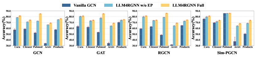
Figure 3. Performance comparison in different settings against Mettack with a 20% perturbation rate.

5.2.2. Against DICE.

To verify the defense generalization capability of LLM4RGNN, we also evaluate its effectiveness against another non-targeted attack, DICE (waniek2018hiding, ). Notably, DICE is not involved in the construction process of the instruction dataset. Considering that DICE is not as effective as Mettack, we set higher perturbation rates of 10%, 20% and 40%. The results are reported in Table 2 and Table 4. Similar to the results under Mettack, LLM4RGNN consistently improves the robustness across various GNNs and is superior to other robust GNN frameworks. For GCN, GAT, RGCN and Simp-GCN, LLM4RGNN on average brings 8.2%, 8.8%, 8.1% and 6.5% relative improvements in accuracy on five datasets. Remarkably, even in some cases where the perturbation ratio increases to 40%, the accuracy of GNNs is better than that on the clean graph.

5.2.3. Against Nettack.

Different from non-targeted attacks, targeted attacks specifically focus on a particular node $v$, aiming to fool GNNs into misclassifying $v$. We employ the SOTA targeted attack, Nettack (zugner2018adversarial, ). Following previous work (zhu2019robust, ), we select nodes with a degree greater than 10 as the target nodes, and vary the number of perturbations applied to the targeted node from 0 to 5 with a step of 1, to generate attacked structures. The results are reported in Table 6 and Table 5. Similar to the results under the Mettack and DICE, LLM4RGNN not only consistently improves the robustness of various GNNs, but also surpasses existing robust GNN frameworks, exhibiting exceptional resistance to Nettack.

Table 6. Node classification accuracy ($\%\pm\sigma$) under targeted attack (Nettack). The best results are in bold.

	Dataset Ptb Num	STABLE	HANG-quad	LLM4RGNN
Cora	0	$\mathbf{88.03_{\pm 2.24}}$	$78.42_{\pm 4.13}$	$87.50_{\pm 1.79}$
	1	$\mathbf{86.05_{\pm 2.14}}$	$77.89_{\pm 2.41}$	${85.79_{\pm 1.75}}$
	2	${84.08_{\pm 1.61}}$	$78.29_{\pm 3.44}$	$\mathbf{85.66_{\pm 2.08}}$
	3	$82.63_{\pm 2.19}$	$76.32_{\pm 4.20}$	$\mathbf{84.47_{\pm 1.15}}$
	4	$79.74_{\pm 2.37}$	$75.00_{\pm 3.06}$	$\mathbf{84.61_{\pm 2.04}}$
	5	$75.13_{\pm 2.24}$	$74.61_{\pm 3.68}$	$\mathbf{84.08_{\pm 1.61}}$
Citeseer	0	$\mathbf{87.08_{\pm 0.75}}$	$79.23_{\pm 3.53}$	$86.77_{\pm 1.02}$
	1	$86.46_{\pm 1.15}$	$78.77_{\pm 2.98}$	$\mathbf{86.46_{\pm 0.62}}$
	2	$84.31_{\pm 1.66}$	$78.15_{\pm 3.56}$	$\mathbf{85.38_{\pm 1.03}}$
	3	$81.54_{\pm 1.54}$	$80.15_{\pm 1.28}$	$\mathbf{86.00_{\pm 0.63}}$
	4	$78.92_{\pm 4.01}$	$78.15_{\pm 3.21}$	$\mathbf{86.00_{\pm 0.83}}$
	5	$78.31_{\pm 4.10}$	$77.54_{\pm 3.01}$	$\mathbf{86.00_{\pm 1.08}}$

In summary, although we fine-tune the local LLM only based on TAPE-Arxiv23, LLM4RGNN still significantly improves the robustness of GNNs in both cross-dataset (Cora, Citeseer, PubMed, OGBN-Arxiv) and cross-domain (OGBN-Products) scenarios.

5.3. Model Analysis

Table 7. Performance comparison with different LLMs against Mettack with a 20% perturbation rate.

LLM		Cora			Citeseer
		AdvEdge (↓)	ACC (↑) w/o EP	ACC (↑) w/ EP	AdvEdge (↓)	ACC (↑) w/o EP	ACC (↑) w/ EP
Close source	GPT-3.5	$186(3.52\%)$	$73.56_{\pm 0.49}$	$75.36_{\pm 1.73}$	$231(5.47\%)$	$66.69_{\pm 1.04}$	$68.92_{\pm 1.63}$
	GPT-4	$\mathbf{90(1.71\%)}$	$\mathbf{79.83_{\pm 0.31}}$	$\mathbf{81.76_{\pm 0.87}}$	$\mathbf{73(1.73\%)}$	$\mathbf{71.04_{\pm 0.57}}$	$\mathbf{72.81_{\pm 0.60}}$
Open source	Llama2-7B	$156(2.96\%)$	$78.76_{\pm 0.42}$	$80.99_{\pm 0.78}$	$203(4.80\%)$	$69.83_{\pm 0.78}$	$72.86_{\pm 0.93}$
	Llama2-13B	$132(2.50\%)$	$79.00_{\pm 0.30}$	$81.35_{\pm 1.15}$	$93(2.20\%)$	$70.81_{\pm 0.73}$	$72.84_{\pm 0.85}$
	Llama3-8B	$107(2.03\%)$	$\mathbf{79.22_{\pm 0.34}}$	$\mathbf{81.71_{\pm 0.51}}$	$\mathbf{91(2.15\%)}$	$70.85_{\pm 0.64}$	$74.06_{\pm 0.78}$
	Mistral-7B	$\mathbf{102(1.93\%)}$	$78.68_{\pm 0.28}$	$81.41_{\pm 0.77}$	$92(2.18\%)$	$\mathbf{71.07_{\pm 0.35}}$	$\mathbf{74.12_{\pm 0.85}}$

(a) Cora-Mettack-5%.

(b) Cora-Mettack-20%.

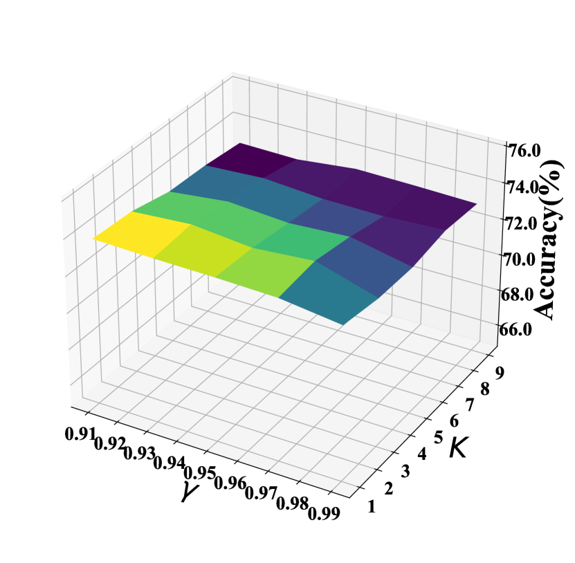
(c) Citeseer-Mettack-5%.

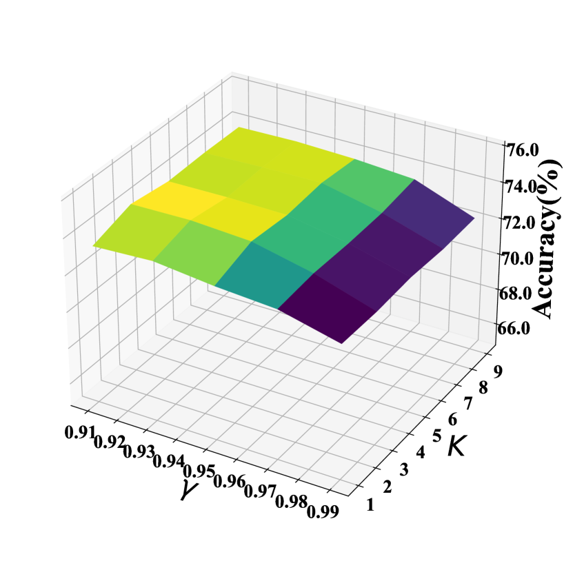
(d) Citeseer-Mettack-20%.

Figure 4. Analysis of the hyper-parameter $\gamma$ and $K$ against Mettack.

5.3.1. Ablation Study.

To assess how the key components of LLM4RGNN benefit the adversarial robustness, we employ Mettack with a perturbation ratio of 20% to generate the attacked structure and conduct ablation experiments. Classical GCN is selected as training GNN. The experiment result is depicted in Figure 3, where ”Vanilla” refers to the setting without any modifications to the attacked structure. The ”w/o EP” variant involves only removing malicious edges by the local LLM, while ”Full” includes both removing malicious edges and adding missing important edges, i.e., our proposed LLM4RGNN. Across all settings, our proposed method consistently outperforms the other settings. Specifically, utilizing the local LLM to identify and remove the majority of malicious edges can significantly reduce the impact of adversarial perturbation, improving the accuracy of GNNs. By further employing the edge predictor to find and add important neighbors for each node, additional information gain is provided to the center nodes, further improving the accuracy of GNNs.

5.3.2. Comparison with Different LLMs.

To evaluate the generalizability of LLM4RGNN across different LLMs, we choose four popular open-source LLMs, including Llama2-7B, Llama2-13B, Llama3-8B and Mistral-7B, as the starting checkpoints of LLM. We also introduce a direct comparison using the closed-source GPT-3.5 and GPT-4 as malicious edge detectors. Additionally, the metric AdvEdge (↓) is introduced to measure the number and proportion of malicious edges remaining after the LLM performs the filtering operation. We report the results of GCN on Cora and Citeseer datasets under Mettack with a perturbation ratio of 20% (generating 1053 malicious edges for Cora and 845 for Citeseer). As reported in Table 7, we have the following observations: (1) The well-tuned local LLMs are significantly superior to GPT-3.5 in identifying malicious edges, and the trained LM-based edge predictor consistently improves accuracy, indicating that the inference capability of GPT-4 is effectively distilled into different LLMs and edge predictors. (2) A stronger open-source LLM yields better overall performance. Among them, the performance of fine-tuned Mistral-7B and Llama3-8B is comparable to that of GPT-4. We provide a comprehensive comparison between Mistral-7B and Llama3-8B in Appendix D.3.

5.3.3. Efficiency Analysis.

In LLM4RGNN, using 26,000 samples to fine-tune the local LLM is a one-time process, controlled within 6 hours. The edge predictor is only a lightweight MLP, with training time on each dataset controlled within 1 minute. Furthermore, LLM4RGNN does not increase the complexity compared with existing robust GNNs framework (li2022reliable, ; jin2020graph, ). The complexity of LLM inferring edge relationships is $O(\mathcal{|E|})$, and the edge predictor is $O({|\mathcal{V}|}^{2})$, and their inference processes are parallelizable. We provide the average time for LLM to infer one edge and for the lightweight edge predictor to infer one node in Table 8. Overall, the average inference time for the local LLM and the edge predictor is 0.7s and 0.2s, respectively, which is acceptable. Each experiment’s total inference time is controlled within 90 minutes.

Table 8. Average inference times (s) for different datasets.

Component	Cora	Citeseer	Products	Pubmed	Arxiv
Local LLM	0.54	0.57	0.63	0.64	1.12
Edge Predictor	0.05	0.06	0.24	0.31	0.25

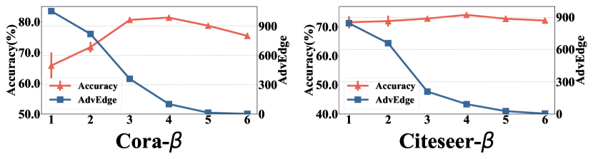
Figure 5. Analysis of hyper-parameter $\beta$ against Mettack-20%.

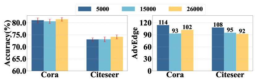
Figure 6. Analysis of instances number against Mettack-20%.

5.4. Hyper-parameter Analysis

We conduct hyper-parameter analysis on the probability threshold $\lambda$, the maximum number of important edges $K$, the purification threshold $\beta$, and the number of instances used in tuning LLMs.

First, we present the accuracy of LLM4RGNN under different combinations of $\lambda$ and $K$ in Figure 4. The results indicate that the accuracy of LLM4RGNN varies minimally across different hyper-parameter settings, demonstrating its insensitivity to the hyper-parameters $\lambda$ and $K$. More results are presented in Appendix D.2.

Besides, we report the accuracy and AdvEdge of LLM4RGNN under different $\beta$, the purification threshold of whether an edge is preserved or not. The results are shown in Figure 5. When the $\beta$ is set to 4, most malicious edges can be identified and achieve optimal performance. This is because a low $\beta$ cannot effectively identify malicious edges, while a high $\beta$ may delete more malicious edges but could also remove some useful edges.

Lastly, we also analyze the effectiveness of LLM4RGNN under different numbers of instances. Specifically, we set the number of instances for tuning the local LLM to 5000, 15000 and 26000, respectively. The results are shown in Figure 6. Remarkably, with only 5000 instances, the tuned local LLM can effectively identify malicious edges, surpassing the current SOTA method. This also indicates that the excellent robustness of LLM4RGNN can be achieved on a lower budget, approximately $80.

6   Conclusion

In this paper, we first explore the potential of LLMs on the graph adversarial robustness. Specifically, we propose a novel LLM-based robust graph structure inference framework, LLM4RGNN, which distills the inference capability of GPT-4 into a local LLM for identifying malicious edges and an LM-based edge predictor for finding missing important edges, to efficiently purify attacked graph structure, making GNNs more robust. Extensive experiments demonstrate that LLM4RGNN significantly improves the adversarial robustness of GNNs and achieves SOTA defense result. Considering there are some graphs that lack textual information, a future plan is to extend LLM4RGNN to graphs without text.

Appendix A Related Work

A.1. Adversarial Attacks and Defenses on Graph

It has been demonstrated in extensive studies (li2022revisiting, ; waniek2018hiding, ; mujkanovic2022defenses, ; jin2021adversarial, ) that attackers can catastrophically degrade the performance of GNNs by maliciously perturbing the graph structure. For example, the Nettack (zugner2018adversarial, ) is the first study of adversarial attacks on graph data, which preserves degree distribution and imposes constraints on feature co-occurrence to generate small deliberate perturbations. Subsequently, the Mettack (zugner_adversarial_2019, ) utilizes the meta-learning while the Minmax and PGD (xu2019topology, ) attacks utilize projected gradient descent, to solve the bilevel problem underlying poisoning attacks.

Threatened by adversarial attacks, many methods (gosch2023revisiting, ; huang2023robust, ; li2023boosting, ; gosch2024adversarial, ) have been proposed to defend against adversarial attacks. These methods can mainly be categorized into model-centric and data-centric. The methods of model-centric improve the robustness through model enhancement, either by robust training schemes (e.g., adversarial training (li2023boosting, ; gosch2024adversarial, )) or designing new model architectures (e.g., RGCN (zhu2019robust, ), HANG (zhao2024adversarial, ), Mid-GCN(huang2023robust, )). The methods of data-centric typically focus on flexible data processing to improve the robustness of GNNs. By treating the attacked topology as noisy, defenders primarily purify graph structures by calculating various similarities between node embeddings (wu2019adversarial, ; jin2020graph, ; zhang2020gnnguard, ; li2022reliable, ; entezari2020all, ). For example, ProGNN (jin2020graph, ) jointly trains GNN’s parameters and learns a clean adjacency matrix with graph properties. STABLE (li2022reliable, ) is a pre-training model, which is specifically designed to learn effective representations to refine graph quality. The above methods have received considerable attention in enhancing the robustness of GNNs.

A.2. LLMs for Graphs

Recently, Large Language models (LLMs) have been widely employed in graph-related tasks, which outperform traditional GNN-based methods and yield SOTA performance. According to the role played by LLMs in graph-related tasks, some methods utilize LLMs as an enhancer (he2023harnessing, ; liu2023one, ; zhang2024graphtranslator, ), where LLMs are used to enhance the quality of node features. Some methods directly utilize LLMs as a predictor (wang2024can, ; chen2024exploring, ; zhao2024gimlet, ; huang2023llms, ), where the graph structure is described in natural language for input to LLMs for prediction. Additionally, some methods employ LLMs as an annotator (chen2023label, ), generator (yu2023empower, ), and controller (wang2023graph, ). Although GraphEdit (guo2024graphedit, ) utilizes LLMs for graph structure learning, it focuses on identifying noisy connections in original graphs, rather than addressing adversarial robustness problem in graphs. In this paper, we adopt LLM as a defender, which utilizes LLMs to purify attacked graph structures, making GNNs more robust.

Appendix B Implementation Details of Baseline in Section 3

For all baselines, we use their original code and the default hyper-parameter settings in the authors’ implementation. The sources are listed as follows:

• TAPE: TAPE Repository

• OFA-Llama2-7B/SBert: OneForAll Repository

• GCN-Llama2-7B/SBert/e5-large: Graph-LLM Repository

Appendix C Experiment Details

C.1. Datasets

In this paper, we use the TAPE-Arxiv23 (he2023harnessing, ) that have up-to-date and rich texts to construct the instruction dataset, and use the following popular datasets commonly adopted for node classifications: Cora (mccallum2000automating, ), Citeseer (giles1998citeseer, ), Pubmed (sen2008collective, ), OGBN-Arxiv (hu2020open, ) and OGBN-Products (hu2020open, ).

Note that for OGBN-Arxiv, given its large scale with 169,343 nodes and 1,166,243 edges, we adopt a node sampling strategy (hamilton2017inductive, ) to obtain a subgraph containing 14,167 nodes and 33,502 edges. For the larger OGBN-Products, which have 2 million nodes and 61 million edges, we used the same sampling technique to construct a subgraph containing 12,394 nodes and 29,676 edges. We give a detailed description of each dataset in Table 9. The sources of datasets are listed as follows:

• Cora, Pubmed, OGBN-Arxiv, TAPE-Arxiv23: TAPE Repository (MIT license)

• OGBN-Products: LLM-Structured-Data Repository (MIT license)

• Citeseer: Graph-LLM Repository (MIT license)

Table 9. Dataset descriptions.

Dataset	#Nodes	#Edges	#Classes	#Features	Method	Description
Cora	2,708	5,429	7	1,433	BoW	After stemming and removing stopwords, there is a vocabulary of size 1,433 unique words. All words with a document frequency of less than 10 were removed.
Citeseer	3,186	4,225	6	3,113	BoW	Remove stopwords and words that appear fewer than 10 times in the document, then use a 0/1-valued word vector to represent the presence of corresponding words in the dictionary.
PubMed	19,717	44,338	3	500	TF-IDF	Each publication in the dataset is described by a TF/IDF weighted word vector from a dictionary which consists of 500 unique words.
OGBN-Arxiv (subset)	14,167	33,520	40	128	skip-gram	The embeddings of individual words are computed by running the skip-gram model (mikolov2013distributed, ) over the MAG (wang2020microsoft, ) corpus.
OGBN-Product (subset)	12,394	29,676	47	100	BoW	Node features are generated by extracting BoW features from the product descriptions followed by a Principal Component Analysis to reduce the dimension to 100.
TAPE-Arxiv23	46,198	78,548	40	300	word2vec	The embeddings of individual words are computed by running the word2vec model.

C.2. Baselines

• GCN: GCN is a popular graph convolutional network based on spectral theory.

• GAT: GAT is composed of multiple attention layers, which can learn different weights for different nodes in the neighborhood. It is often used as a baseline for defending against adversarial attacks.

• RGCN: RGCN models node representations as Gaussian distributions to mitigate the impact of adversarial attacks, and employs an attention mechanism to penalize nodes with high variance.

• Simp-GCN: SimpGCN employs a $k$NN graph to maintain the proximity of nodes with similar features in the representation space and uses self-learned regularization to preserve the remoteness of nodes with differing features.

• ProGNN: ProGNN adapts three regularizations of graphs, i.e., feature smoothness, low-rank, and sparsity, and learns a clean adjacency matrix to defend against adversarial attacks.

• STABLE: STABLE is a pre-training model, which is specifically designed to learn effective representations to refine graph structures.

• HANG-quad: HANG-quad incorporates conservative Hamiltonian flows with Lyapunov stability to various GNNs, to improve their robustness against adversarial attacks.

• GraphEdit: GraphEdit utilizes LLMs to identify noisy connections and uncover implicit relations among non-connected nodes in the original graph.

C.3. Implementation Details

We use DeepRobust, an adversarial attack repository, to implement all the attack methods as well as GCN, GAT, RGCN, and Sim-PGCN. We implement ProGNN, STABLE, and HANG-quad with the code provided by the authors.

For each graph, following existing works (jin2020graph, ; li2022reliable, ), we randomly split the nodes into 10% for training, 10% for validation, and 80% for testing. We generate attacks on each graph according to the perturbation rate, and all the hyper-parameters in attack methods are the same as the authors’ implementation.

For LLM4RGNN, we use Mistral-7B as our local LLM. Based on GPT-4, we construct approximately 26,000 instances for tuning LLMs and use the LoRA method to achieve parameter-efficient fine-tuning. To address the potential problem of label imbalance in training LM-based edge predictor, we select the $4000$ node pairs with the lowest cosine similarity to construct the candidate set. We set the hyper-parameters as follows: For local LLMs, when no purification occurs, the purification threshold $\beta$ is fixed at 2 to prevent deleting too many edges; otherwise, it is set to 4. For LM-based edge predictor, the threshold $\gamma$ is tuned from $\{0.91,0.93,0.95,0.97,0.99\}$ and the number of edges $K$ is tuned from $\{1,3,5,7,9\}$.

To facilitate fair comparisons, we tune the parameters of various baselines using a grid search strategy. Unless otherwise specified, we adopt the default parameter setting in the author’s implementation. For GCN, we set the hidden size is 256 for the OGBN-Arxiv, and 16 for other datasets. For GAT, the hidden size is 128 for the OGBN-Arxiv and 8 for other datasets. For RGCN and Sim-PGCN, the hidden size is 256 for the OGBN-Arxiv and 128 for other datasets. For Sim-PGCN, we tune the weighting parameter $\lambda$ is searched from $\{0.1,0.5,1,5,10,50,100\}$ and $\gamma$ is searched from $\{0.01,0.1\}$. For Pro-GNN, we use the default hyper-parameter settings in the authors’ implementation. For STABLE, we tune the Jaccard Similarity threshold $t_{1}$ from $\{0.0,0.01,0.02,0.03,0.04,0.05\}$, $k$ is tuned from $\{1,3,5,7,11,13\}$, $\alpha$ is tuned from $-0.5$ to $3$. For HANG_quad, we tune the time from $\{3,6,8,15,20,25\}$, the hidden size from $\{16,32,64,128\}$, and dropout from $\{0.2,0.4,0.6,0.8\}$. For all experiments, we select the optimal hyper-parameters on the validation set and apply them to the test set. The sources of baselines are listed as follows:

• GCN: DeepRobust GCN

• GAT: DeepRobust GAT

• RGCN: DeepRobust RGCN

• Sim-PGCN: DeepRobust Sim-PGCN

• ProGNN: ProGNN Repository

• STABLE: STABLE Repository

• HANG-quad: HANG-quad Repository

• GraphEdit: GraphEdit Repository

C.4. Computing Environment and Resources

The checkpoint of the local LLM and source code will be publicly available after the review. The implementation of the proposed LLM4RGNN utilized the PyG module. The experiments are conducted in a computing environment with the following specifications:

• OS: Linux ubuntu 5.15.0-102-generic.

• CPU: Intel(R) Xeon(R) Platinum 8358 CPU @ 2.60GHz.

• GPU: NVIDIA A800 80GB.

Appendix D More Experiment Results

Table 10. Performance comparison between Mistral-7B and Llama3-8B against Mettack.

Dataset	Ptb Rate	AdvEdge (↓)		ACC (↑) w/o EP		ACC (↑) Full
		Mistral-7B	Llama3-8B	Mistral-7B	Llama3-8B	Mistral-7B	Llama3-8B
Cora	$0\%$	-	-	$\mathbf{83.78_{\pm 0.38}}$	$83.72_{\pm 0.30}$	$84.13_{\pm 0.33}$	$\mathbf{84.34_{\pm 0.56}}$
	$5\%$	$\mathbf{28(0.53\%)}$	$30(0.57\%)$	$80.48_{\pm 0.19}$	$\mathbf{80.60_{\pm 0.27}}$	$81.76_{\pm 0.69}$	$\mathbf{81.98_{\pm 0.55}}$
	$10\%$	$\mathbf{60(1.14\%)}$	$63(1.19\%)$	$79.83_{\pm 0.43}$	$\mathbf{79.96_{\pm 0.39}}$	$\mathbf{81.80_{\pm 0.76}}$	$81.77_{\pm 0.44}$
	$20\%$	$\mathbf{102(1.93\%)}$	$107(2.03\%)$	$78.68_{\pm 0.28}$	$\mathbf{79.22_{\pm 0.34}}$	$81.41_{\pm 0.77}$	$\mathbf{81.71_{\pm 0.51}}$
Citeseer	$0\%$	-	-	$73.39_{\pm 0.69}$	$\mathbf{73.41_{\pm 0.65}}$	$\mathbf{74.20_{\pm 0.56}}$	$73.84_{\pm 0.50}$
	$5\%$	$30(0.71\%)$	$\mathbf{25(0.59\%)}$	$72.17_{\pm 0.57}$	$\mathbf{72.44_{\pm 0.52}}$	$\mathbf{73.94_{\pm 0.56}}$	$73.28_{\pm 1.19}$
	$10\%$	$55(1.30\%)$	$\mathbf{47(1.11\%)}$	$\mathbf{71.50_{\pm 0.59}}$	$71.32_{\pm 0.58}$	$\mathbf{73.62_{\pm 0.39}}$	$73.20_{\pm 0.68}$
	$20\%$	$92(2.18\%)$	$\mathbf{91(2.15\%)}$	$\mathbf{71.07_{\pm 0.35}}$	$70.85_{\pm 0.64}$	$\mathbf{74.12_{\pm 0.85}}$	$74.06_{\pm 0.78}$

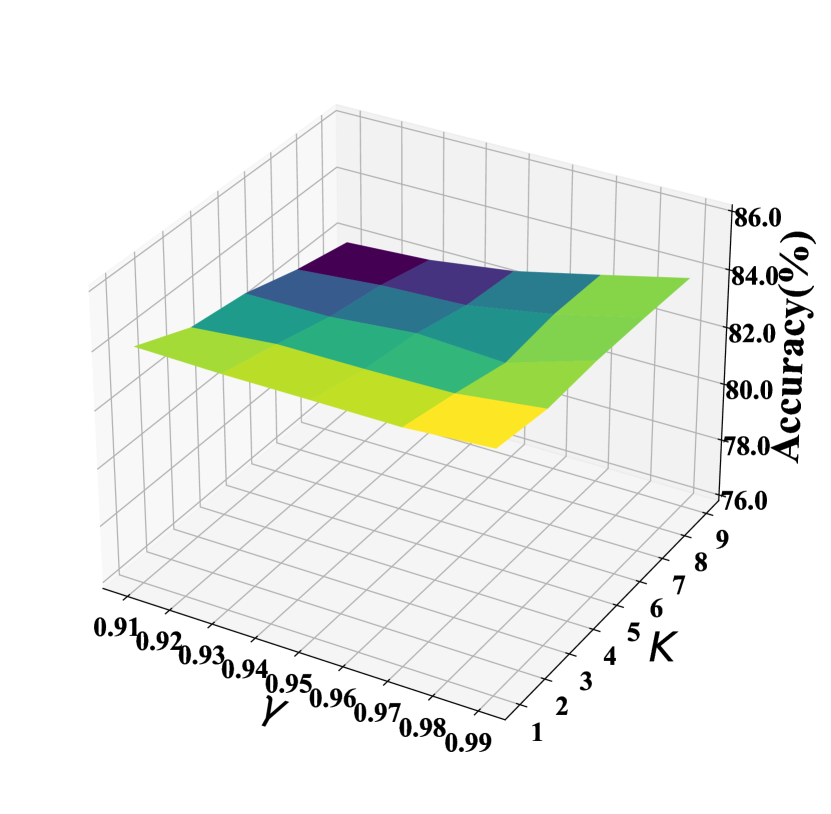
(a) Clean Cora.

(b) Cora-Mettack-10%.

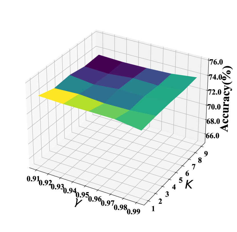
(c) Clean Citeseer.

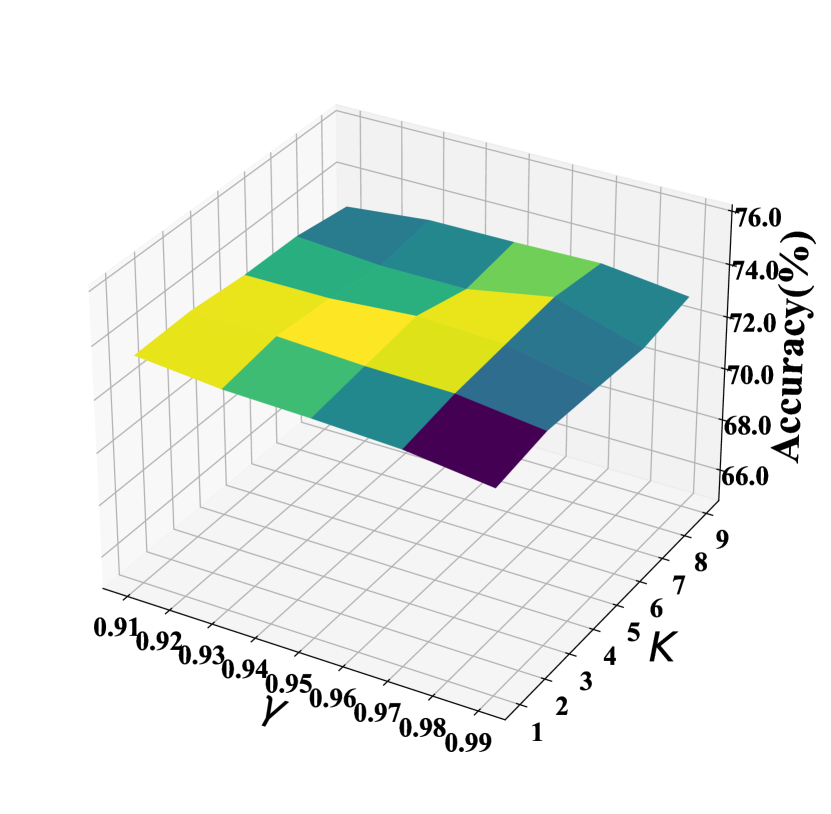
(d) Citeseer-Mettack-10%.

Figure 7. Analysis of the hyper-parameter $\gamma$ and $K$.

D.1. Inductive Poisoning Atatck

We further verify the generalization ability of LLM4RGNN under inductive poisoning attacks. We conduct inductive experiments with Mettack on the Cora and Citeseer datasets. Specifically, we randomly split the data into training, validation, and test sets with a 1:8:1 ratio. During training, we ensure the removal of test nodes and their connected edges from the graph. We perform Mettack attacks on the validation set, purify the attacked graph using LLM4RGNN, and use the purified graph to train GNNs. The trained GNNs are then predicted on the clean test set. As shown in Table 11, we only report the baselines that support the inductive setting. Experimental results show that under the inductive setting, LLM4RGNN not only consistently improves the robustness of various GNNs but also surpasses the robust GCN framework HANG-quad, demonstrating its superior defensive capability in the inductive setting.

Table 11. Node classification accuracy ($\%\pm\sigma$) under Inductive Mettack. The best results are in bold.

	Dataset Ptb Rate	HANG-quad	GCN		GAT
			Vanilla	LLM4RGNN	Vanilla	LLM4RGNN
Cora	0%	$82.09\pm 0.40$	$84.36\pm 0.28$	$84.25\pm 0.16$	$84.35\pm 0.62$	$\mathbf{84.39\pm 0.61}$
	5%	$75.85\pm 0.67$	$77.35\pm 1.56$	$83.17\pm 0.17$	$81.20\pm 0.93$	$\mathbf{83.68\pm 0.26}$
	10%	$70.95\pm 1.26$	$72.79\pm 1.49$	$83.02\pm 0.34$	$78.55\pm 1.12$	$\mathbf{83.48\pm 0.49}$
	20%	$58.81\pm 1.99$	$61.56\pm 2.64$	$82.69\pm 0.65$	$67.65\pm 2.69$	$\mathbf{83.14\pm 0.69}$
Citeseer	0%	$73.15\pm 0.94$	$73.76\pm 0.34$	$74.07\pm 0.51$	$73.84\pm 0.57$	$\mathbf{74.26\pm 0.69}$
	5%	$71.50\pm 0.55$	$70.60\pm 0.56$	$\mathbf{73.35\pm 0.35}$	$72.47\pm 0.82$	$73.25\pm 0.91$
	10%	$69.42\pm 0.64$	$67.64\pm 0.73$	$72.68\pm 0.41$	$71.11\pm 1.02$	$\mathbf{73.25\pm 0.40}$
	20%	$67.90\pm 1.21$	$61.35\pm 1.35$	$72.54\pm 0.36$	$65.76\pm 2.85$	$\mathbf{73.32\pm 0.52}$

D.2. More Hyper-parameter Sensitivity

We conduct more hyper-parameter experiments on the probability threshold $\lambda$ and the number of important edges $K$. The result is shown in Figure 7, demonstrating that the performance of the proposed LLM4RGNN is stable under various parameter configurations and consistently outperforms existing SOTA methods.

D.3. Comparative Experiment between Llama3-8B and Mistral-7B

In Section 5.3.2, the newly released Llama3-8B and Mistral-7B achieved close performance. Considering that Llama3-8B is released after all experiments are completed, we report additional comparative experiments between Mistral-7B and Llama3-8B. According to Table 10, we observe that both the well-tuned Mistral-7B and Llama3-8B can effectively identify malicious edges, and the performance gap between them is negligible.

Table 12. Against Mettack-20%, node classification accuracy ($\%\pm\sigma$) of LLM4RGNN under different text quality.

	Dataset Ptb Rate	GCN	GAT	RGCN	Sim-PGCN
Cora	0%	$81.41\pm 0.77$	$81.00\pm 0.98$	$81.39\pm 0.44$	$81.20\pm 0.63$
	10%	$80.41\pm 0.71$	$80.72\pm 0.49$	$80.54\pm 0.61$	$81.14\pm 0.47$
	20%	$79.86\pm 0.42$	$80.12\pm 0.69$	$80.14\pm 0.80$	$80.75\pm 0.40$
	40%	$79.54\pm 1.51$	$79.88\pm 1.18$	$80.07\pm 1.22$	$80.18\pm 1.11$
Citeseer	0%	$74.12\pm 0.85$	$73.94\pm 0.67$	$74.04\pm 0.70$	$73.70\pm 0.64$
	10%	$73.21\pm 0.98$	$73.65\pm 0.71$	$73.10\pm 1.01$	$73.68\pm 0.82$
	20%	$73.55\pm 0.66$	$73.02\pm 0.66$	$73.30\pm 0.93$	$73.84\pm 0.78$
	40%	$72.67\pm 0.70$	$72.62\pm 1.09$	$73.18\pm 0.94$	$73.47\pm 0.55$

D.4. The Impact of Text Quality

Considering that LLM4RGNN relies on textual information for reasoning, we further analyze the impact of node text quality on the effectiveness of LLM4RGNN. Specifically, against the worst-case scenario of 20% Mettack, we further add random text replacement perturbations to the Cora and Citeseer datasets to reduce the text quality of nodes. As shown in Table 12, experimental results show that under 10%, 20%, and 40% text perturbations, the performance of LLM4RGNN only decreases by an average of 0.54%, 0.77%, and 1.14%, respectively. Its robustness consistently surpasses that of existing robust GNN frameworks, demonstrating that LLM4RGNN maintains superior robustness even with lower text quality. One possible explanation is that LLMs have strong robustness to text perturbations (chang2024survey, ), and LLM4RGNN fully inherits this capability.

Appendix E Case Study

In this section, we show some cases using GPT-4 and well-tuned local LLMs (Mistral-7B) to infer the relationships between nodes. It can be observed that the well-tuned Mistral-7B can achieve the edge relation inference ability of GPT-4. They infer the edge relations and provide analysis by discussing the background, problems, methods, and applications of two nodes.

E.1. TAPE-Arxiv23 (GPT-4)

E.2. Cora (Mistral-7B)

References

- (1) Josh Achiam, Steven Adler, Sandhini Agarwal, et al. Gpt-4 technical report. arXiv preprint arXiv:2303.08774, 2023.
- (2) Yupeng Chang, Xu Wang, Jindong Wang, et al. A survey on evaluation of large language models. ACM Transactions on Intelligent Systems and Technology, 2024.
- (3) Zhikai Chen, Haitao Mao, Hang Li, et al. Exploring the potential of large language models (llms) in learning on graphs. ACM SIGKDD Explorations Newsletter, 2024.
- (4) Zhikai Chen, Haitao Mao, Hongzhi Wen, et al. Label-free node classification on graphs with large language models (llms). In The Twelfth International Conference on Learning Representations, 2023.
- (5) Negin Entezari, Saba A Al-Sayouri, Amirali Darvishzadeh, et al. All you need is low (rank) defending against adversarial attacks on graphs. In Proceedings of the 13th international conference on web search and data mining, 2020.
- (6) C Lee Giles, Kurt D Bollacker, and Steve Lawrence. Citeseer: An automatic citation indexing system. In Proceedings of the third ACM conference on Digital libraries, 1998.
- (7) Lukas Gosch, Simon Geisler, Daniel Sturm, et al. Adversarial training for graph neural networks: Pitfalls, solutions, and new directions. Advances in Neural Information Processing Systems, 2024.
- (8) Lukas Gosch, Daniel Sturm, Simon Geisler, et al. Revisiting robustness in graph machine learning. arXiv preprint arXiv:2305.00851, 2023.
- (9) Zirui Guo, Lianghao Xia, Yanhua Yu, et al. Graphedit: Large language models for graph structure learning. arXiv preprint arXiv:2402.15183, 2024.
- (10) Will Hamilton, Zhitao Ying, and Jure Leskovec. Inductive representation learning on large graphs. Advances in neural information processing systems, 2017.
- (11) Zellig S Harris. Distributional structure. Word, 1954.
- (12) Xiaoxin He, Xavier Bresson, Thomas Laurent, et al. Harnessing explanations: Llm-to-lm interpreter for enhanced text-attributed graph representation learning. In The Twelfth International Conference on Learning Representations, 2023.
- (13) Weihua Hu, Matthias Fey, Marinka Zitnik, et al. Open graph benchmark: Datasets for machine learning on graphs. Advances in neural information processing systems, 2020.
- (14) Jin Huang, Xingjian Zhang, Qiaozhu Mei, et al. Can llms effectively leverage graph structural information: When and why, 2023.
- (15) Jincheng Huang, Lun Du, Xu Chen, et al. Robust mid-pass filtering graph convolutional networks. In Proceedings of the ACM Web Conference 2023, 2023.
- (16) Albert Q Jiang, Alexandre Sablayrolles, Arthur Mensch, et al. Mistral 7b. arXiv preprint arXiv:2310.06825, 2023.
- (17) Wei Jin, Tyler Derr, Yiqi Wang, et al. Node similarity preserving graph convolutional networks. In Proceedings of the 14th ACM international conference on web search and data mining, 2021.
- (18) Wei Jin, Yaxing Li, Han Xu, et al. Adversarial attacks and defenses on graphs. ACM SIGKDD Explorations Newsletter, 2021.
- (19) Wei Jin, Yao Ma, Xiaorui Liu, et al. Graph structure learning for robust graph neural networks. In Proceedings of the 26th ACM SIGKDD international conference on knowledge discovery & data mining, 2020.
- (20) Thomas N Kipf and Max Welling. Semi-supervised classification with graph convolutional networks. arXiv preprint arXiv:1609.02907, 2016.
- (21) Kuan Li, YiWen Chen, Yang Liu, et al. Boosting the adversarial robustness of graph neural networks: An ood perspective. In The Twelfth International Conference on Learning Representations, 2023.
- (22) Kuan Li, Yang Liu, Xiang Ao, et al. Reliable representations make a stronger defender: Unsupervised structure refinement for robust gnn. In Proceedings of the 28th ACM SIGKDD Conference on Knowledge Discovery and Data Mining, 2022.
- (23) Kuan Li, Yang Liu, Xiang Ao, et al. Revisiting graph adversarial attack and defense from a data distribution perspective. In The Eleventh International Conference on Learning Representations, 2022.
- (24) Hao Liu, Jiarui Feng, Lecheng Kong, et al. One for all: Towards training one graph model for all classification tasks. arXiv preprint arXiv:2310.00149, 2023.
- (25) Jiawei Liu, Cheng Yang, Zhiyuan Lu, et al. Towards graph foundation models: A survey and beyond. arXiv preprint arXiv:2310.11829, 2023.
- (26) Chengsheng Mao, Liang Yao, and Yuan Luo. Medgcn: Graph convolutional networks for multiple medical tasks. arXiv preprint arXiv:1904.00326, 2019.
- (27) Andrew Kachites McCallum, Kamal Nigam, Jason Rennie, et al. Automating the construction of internet portals with machine learning. Information Retrieval, 2000.
- (28) Tomas Mikolov, Ilya Sutskever, Kai Chen, et al. Distributed representations of words and phrases and their compositionality. Advances in neural information processing systems, 2013.
- (29) Felix Mujkanovic, Simon Geisler, Stephan Günnemann, et al. Are defenses for graph neural networks robust? Advances in Neural Information Processing Systems, 2022.
- (30) Nils Reimers and Iryna Gurevych. Sentence-bert: Sentence embeddings using siamese bert-networks. arXiv preprint arXiv:1908.10084, 2019.
- (31) Stephen Robertson. Understanding inverse document frequency: on theoretical arguments for idf. Journal of documentation, 2004.
- (32) Prithviraj Sen, Galileo Namata, Mustafa Bilgic, et al. Collective classification in network data. AI magazine, 2008.
- (33) Lichao Sun, Yingtong Dou, Carl Yang, et al. Adversarial attack and defense on graph data: A survey. IEEE Transactions on Knowledge and Data Engineering, 2022.
- (34) Hugo Touvron, Thibaut Lavril, Gautier Izacard, et al. Llama: Open and efficient foundation language models. arXiv preprint arXiv:2302.13971, 2023.
- (35) Petar Veličković, Guillem Cucurull, Arantxa Casanova, et al. Graph attention networks. arXiv preprint arXiv:1710.10903, 2017.
- (36) Haishuai Wang, Yang Gao, Xin Zheng, et al. Graph neural architecture search with gpt-4. arXiv preprint arXiv:2310.01436, 2023.
- (37) Heng Wang, Shangbin Feng, Tianxing He, et al. Can language models solve graph problems in natural language? Advances in Neural Information Processing Systems, 2024.
- (38) Jianian Wang, Sheng Zhang, Yanghua Xiao, et al. A review on graph neural network methods in financial applications. arXiv preprint arXiv:2111.15367, 2021.
- (39) Kuansan Wang, Zhihong Shen, Chiyuan Huang, et al. Microsoft academic graph: When experts are not enough. Quantitative Science Studies, 2020.
- (40) Marcin Waniek, Tomasz P Michalak, Michael J Wooldridge, et al. Hiding individuals and communities in a social network. Nature Human Behaviour, 2018.
- (41) Huijun Wu, Chen Wang, Yuriy Tyshetskiy, et al. Adversarial examples on graph data: Deep insights into attack and defense. arXiv preprint arXiv:1903.01610, 2019.
- (42) Zonghan Wu, Shirui Pan, Fengwen Chen, et al. A comprehensive survey on graph neural networks. IEEE transactions on neural networks and learning systems, 2020.
- (43) Kaidi Xu, Hongge Chen, Sijia Liu, et al. Topology attack and defense for graph neural networks: An optimization perspective. arXiv preprint arXiv:1906.04214, 2019.
- (44) Xiaohan Xu, Ming Li, Chongyang Tao, et al. A survey on knowledge distillation of large language models. arXiv preprint arXiv:2402.13116, 2024.
- (45) Shukang Yin, Chaoyou Fu, Sirui Zhao, et al. A survey on multimodal large language models. arXiv preprint arXiv:2306.13549, 2023.
- (46) Jianxiang Yu, Yuxiang Ren, Chenghua Gong, et al. Empower text-attributed graphs learning with large language models (llms). arXiv preprint arXiv:2310.09872, 2023.
- (47) Mengmei Zhang, Mingwei Sun, Peng Wang, et al. Graphtranslator: Aligning graph model to large language model for open-ended tasks. arXiv preprint arXiv:2402.07197, 2024.
- (48) Xiang Zhang and Marinka Zitnik. Gnnguard: Defending graph neural networks against adversarial attacks. Advances in neural information processing systems, 2020.
- (49) Haiteng Zhao, Shengchao Liu, Ma Chang, et al. Gimlet: A unified graph-text model for instruction-based molecule zero-shot learning. Advances in Neural Information Processing Systems, 2024.
- (50) Kai Zhao, Qiyu Kang, Yang Song, et al. Adversarial robustness in graph neural networks: A hamiltonian approach. Advances in Neural Information Processing Systems, 2024.
- (51) Wayne Xin Zhao, Kun Zhou, Junyi Li, et al. A survey of large language models. arXiv preprint arXiv:2303.18223, 2023.
- (52) Qinkai Zheng, Xu Zou, Yuxiao Dong, et al. Graph robustness benchmark: Benchmarking the adversarial robustness of graph machine learning. Neural Information Processing Systems Track on Datasets and Benchmarks 2021, 2021.
- (53) Dingyuan Zhu, Ziwei Zhang, Peng Cui, et al. Robust graph convolutional networks against adversarial attacks. In Proceedings of the 25th ACM SIGKDD international conference on knowledge discovery & data mining, 2019.
- (54) Daniel Zügner, Amir Akbarnejad, and Stephan Günnemann. Adversarial attacks on neural networks for graph data. In Proceedings of the 24th ACM SIGKDD international conference on knowledge discovery & data mining, 2018.
- (55) Daniel Zügner and Stephan Günnemann. Adversarial attacks on graph neural networks via meta learning. In International Conference on Learning Representations (ICLR), 2019.