Convergence Framework of Deep Learning-based Hybrid Iterative Methods and the Application to Designing a Fourier Neural Solver for Parametric PDEs
Abstract
Recently, deep learning-based hybrid iterative methods (DL-HIM) have emerged as a promising approach for designing fast neural solvers to tackle large-scale sparse linear systems. DL-HIM combine the smoothing effect of simple iterative methods with the spectral bias of neural networks, which allows them to effectively eliminate both high-frequency and low-frequency error components. However, their efficiency may decrease if simple iterative methods can not provide effective smoothing, making it difficult for the neural network to learn mid-frequency and high-frequency components. This paper first establishes a convergence analysis framework for general DL-HIM from a spectral viewpoint, concluding that under reasonable assumptions, DL-HIM exhibit a convergence rate independent of grid size and physical parameters . To meet these assumptions, we design a neural network from an eigen perspective, focusing on learning the eigenvalues and eigenvectors corresponding to error components that simple iterative methods struggle to eliminate. Specifically, the eigenvalues are learned by a meta subnet, while the eigenvectors are approximated using Fourier modes with a transition matrix provided by another meta subnet. The resulting DL-HIM, termed the Fourier Neural Solver (FNS), is expected to achieve a -independent convergence rate with the guarantee of universal approximation and the discretization invariant property of the meta subnets. We verify the performance of FNS on four types of linear parametric PDEs.
keywords:
Hybrid iterative method, Neural solver, Preconditioning, Convergence analysis, Spectral bias[a]organization=Hunan Key Laboratory for Computation and Simulation in Science and Engineering, Key Laboratory of Intelligent Computing and Information Processing of Ministry of Education, School of Mathematics and Computational Science, Xiangtan University, city=Xiangtan, postcode=411105, state=Hunan, country=China
1 Introduction
Large-scale sparse linear system of equations
| (1) |
are ubiquitous in scientific and engineering applications, particularly those arising from the discretization of partial differential equations (PDEs). Developing efficient, robust, and adaptive numerical methods to solve these equations remains a significant challenge for researchers in applied mathematics. Iterative methods [1] offer an effective solution for solving such systems. Starting with an initial guess , the simplest form is relaxation
| (2) |
where is the relaxation parameter. This method is known as the Richardson iterative method. Although the computational cost per step is cheap, its convergence rate is quite slow in practical applications. Consequently, various acceleration techniques have been developed. For example, one can select the optimal using Chebyshev polynomials [2]; search for solutions along the conjugate gradient direction instead of the negative gradient direction [3]; introduce the momentum term, such as Nesterov acceleration [4, 5]; split the unknown into blocks for block coordinate descent [6]; split into the sum of different operators for alternating-direction implicit iteration [7]; use information from previous steps, such as Anderson acceleration [8]; and project into the Krylov subspace to find solutions, such as GMRES [9], etc.
However, the convergence speed of these acceleration techniques is still constrained by the condition number of . To mitigate this limitation, preconditioning techniques are introduced
| (3) |
where is called the preconditioner, designed to approximate and should be computationally easy to obtain. Simple preconditioners, such as damped Jacobi, Gauss-Seidel, and successive over-relaxation methods [1], also exhibit slow convergence rates. Commonly used preconditioners include incomplete LU (ILU) factorization [10], multigrid (MG) [11], and domain decomposition methods (DDM) [12]. For example, MG methods are optimal for elliptic problems. In more complex cases, preconditioners are often combined with acceleration methods, such as flexible conjugate gradient (FCG) [13] and flexible GMRES (FGMRES) [14]. However, when dealing with challenging problems, effective methods often require problem-specific parameters that need be determined by experts.
In recent years, deep learning techniques have emerged as innovative approaches to solving PDEs, offering new perspectives in scientific computing. There are three main applications: First, as a universal approximator for solving complex (e.g., high-dimensional) PDEs, known as neural pde [15]. Second, as a discretization-invariant surrogate model for parametric PDEs (PPDE) that maps infinite-dimensional parameter spaces to solution spaces, referred to as the neural operator [16]. Third, in designing fast iterative methods for discretized systems, which we refer to as the neural solver. Neural solvers primarily evolve from two aspects. The first involves automatically learning problem-specific parameters for existing iterative methods. For example, in acceleration techniques, neural networks have been utilized to learn parameters in Chebyshev acceleration for improved smoothing effects [17], or to learn iterative directions in place of conjugate directions [18]. For parameters in preconditioners, neural networks can be used to correct ILU preconditioners [19]; learn smoothers [20, 21, 22], transfer operators [23, 24, 25], coarsening [26, 27, 28] in MG; learn adaptive coarse basis functions [29], interface conditions and interpolation operators [30, 31, 32, 25] in DDM, etc.
The other approach involves combining the traditional preconditioner with the neural network to form the following deep learning-based hybrid iterative method (DL-HIM)
| (4a) | ||||
| (4b) | ||||
The primary motivation is that tends to fit low-frequency functions due to spectral bias [33, 34, 35], while simple preconditioners , such as damped Jacobi and Gauss-Seidel, are effective for eliminating high-frequency error components. We refer to (4a) as the smoothing iteration because it is primarily intended to eliminate oscillatory error components. However, in certain problems, it may not fully achieve this goal, so the term “smoothing iteration” is used in a broader sense, as long as it can reduce some parts of the error. The neural network must be applicable for any . Therefore, it is typically designed as a discretization-invariant neural operator. The iterative method (4) was first proposed in [36], where DeepONet [37] was used as and combined with different preconditioners to test the compressibility of (4) for error components of various frequencies. This approach, referred to as the hybrid iterative numerical transferable solver (HINTS), was later extended to handle different geometries [38] and to solve the Helmholtz equation [39]. Around the same time, the authors of [40] employed local Fourier analysis (LFA) [41] to estimate which frequency components the selected could effectively eliminate. Inspired by the fast Poisson solver [42, 43], they designed based on the fast Fourier transform (FFT) to eliminate error components difficult for to handle. In 2023, the authors of [44] designed a multilevel structure that mimics MG as , with shared parameters across different levels. This approach demonstrated good computational efficiency for convection-diffusion equations. In 2024, the authors of [45] used the SNO [46] as and further accelerated it with FCG. In the same year, the authors of [47] used MIONet [48] as and analyzed the convergence rate of the corresponding DL-HIM for the Poisson equation for the first time. Also in 2024, the author of [49] used a graph neural network to directly approximate as a nonlinear preconditioner for FGMRES.
In this paper, we consider the linear systems arising from discretizing the steady-state linear PPDE
| (5) |
where is the differential operator, is the solution function, is the source term, and is the parameter in a compact space. It is assumed that the equation (5) is well-posed under appropriate boundary conditions. By dividing into a discrete grid and applying numerical discretization methods, such as the finite element method (FEM), we obtain the following linear systems of equations
where and . In many practical scenarios, such as inverse problems, design, optimization, and uncertainty quantification, it is crucial to examine the behavior of the physics-based model across various parameters . In these cases, high-fidelity simulations, which involve solving the linear system multiple times, can become prohibitively expensive. Therefore, we aim to utilize DL-HIM to reduce the computational cost. For simplicity, we omit the superscripts related to specific parameters and consider linear systems (1).
The main contents of this paper are as follows. First, we establish a convergence analysis framework for the general DL-HIM (4) from a spectral perspective. For a diagonalizable matrix , under reasonable assumptions on and , we can obtain a DL-HIM with a convergence rate independent of the mesh size and physical parameters . To ensure that meets its assumptions, we design it from an eigen perspective. Building on our previous work [40], we improve by replacing the use of a Fourier matrix as the eigenvector matrix with a transition matrix that maps from the Fourier modes to the eigenvector basis. By introducing two meta subnets to learn the inverse of the eigenvalues and the transition matrix, we transform the requirements on into requirements on the meta subnets. This approach avoids the constraints of spectral bias, enabling to approximate not only low-frequency error components but also error components that struggles to eliminate. The improved solver, still called Fourier Neural Solver (FNS), is implemented as an end-to-end, differentiable neural solver for linear systems derived from structured grids. We design a reasonable loss function and construct easily accessible and targeted training data to train FNS and test its performance on a variety of classical PDE discrete systems. For random diffusion equations, the selected effectively eliminates high-frequency errors, and a well-trained can learn low-frequency and mid-frequency error components, allowing FNS to achieve a convergence rate independent of physical parameters and grid size. For multi-scale problems, such as discrete systems arising from anisotropic, strong convection, and jumping diffusion equations, FNS can still achieve a convergence rate independent of physical parameters and grid size on small and medium scales with additional help. In summary, the advantages of FNS over other DL-HIM are as follows:
-
(1)
FNS can handle error components with different frequencies. Some DL-HIM [36, 38, 47, 39, 45] train separately, similar to a neural operator. However, the trained tends to capture only low-frequency components due to spectral bias. In contrast, the of FNS, trained in Fourier space, is not affected by spectral bias. It can also automatically learn error components that are difficult for to eliminate because it is trained within (4) in an end-to-end manner.
-
(2)
The training data for FNS is easy to obtain as it does not require solving PDEs. The loss function is designed to ensure that focuses on error components that struggles to eliminate.
-
(3)
The nonlinearity of FNS only exists in the meta subnets; is linear and therefore scale-equivariant. During the iteration process, the input of (residual) can have vastly different scales, and the output (error) should also change proportionally. DL-HIM with nonlinear [50, 36, 38, 39, 45, 49] cannot naturally guarantee this property.
-
(4)
The asymptotic convergence rate of FNS is independent of the right-hand sides (RHS).
The rest of this paper is organized as follows: Section 2 establishes a convergence analysis framework for the general DL-HIM; Section 3 proposes FNS and designs reasonable training data and loss functions under the guidance of convergence analysis; Section 4 conducts numerical experiments on four types of second-order linear PDEs to verify the theoretical analysis; and Section 5 gives a summary and outlook.
2 Convergence framework
The error propagation matrix of (4) is given by
then the iterative method (4) converges if and only if
where denotes the spectral radius. If , (4) will certainly converge as [47]. Next, we analyze the convergence of the smoother and the neural operator from a spectral perspective for a fixed .
2.1 Convergence of the smoother
We use LFA [41] to perform convergence analysis on the smoothing iteration (4a). Define the infinite grid
| (6) |
and the Fourier modes on it
| (7) |
where denotes the Fourier frequencies, which can be restricted to , due to the periodic property
Consider a general discrete operator defined on
| (8) |
where the coefficients , and is a finite index set. When is independent of , the operator corresponds to a Toeplitz matrix, which can be diagonalized using Fourier modes. This leads to the following lemma.
Lemma 1 (Lemma 4.2.1 [11])
For any the Fourier modes are formal eigenfunctions of the discrete operator with constant stencil
| (9) |
where
| (10) |
is called the formal eigenvalue or symbol of .
When depends on , becomes a Fourier matrix symbol rather than a scalar function. The smoothing effect of on different frequencies can still be analyzed through appropriate transformations. For further details, see [51, 52, 53].
Assume that the -th iteration error of (4) is , and is its periodic extension function on the infinite grid . Since form an orthonormal basis for the Fourier space, can be expanded in terms of these bases as
| (11) |
and satisfies Parseval’s identity
| (12) |
Since smoothing iteration (4a) is always implemented as a simple stationary iterative method, the corresponding error propagation matrix can be wirtten down as a discrete operator in the form of (8). Thus,
| (13) |
and applying (4a) to (11) yields
| (14) |
It can be seen that when , the smoothing iteration effectively reduces the error component with frequency . However, when or greater than 1, the corresponding error components decay slowly or may even amplify. Based on this fact, we make the following assumptions.
Assumption 2.1 (Smoothing effect of )
Assume that can be split into , which satisfy
| (15) |
where the smoothing factor and the small positive constant are independent of the mesh size and physical parameters .
Under this assumption, (14) can be decomposed into
| (16) |
2.2 Convergence of the neural operator
Denote the restriction of and on as
then (16) becomes
| (17) |
Applying the neural iteration (4b) to , we have
| (18) | ||||
By computing the norm, we obtain
| (19) |
Next, we do an estimate on . To achieve this, assume that can be diagonalized
| (20) |
where is a diagonal matrix, whose diagonal entries are the eigenvalues , and the -th column of is the corresponding eigenvector . Note that can be linearly expressed by these eigenvectors
| (21) |
where . Using the eigendecomposition (20) of , we have
| (22) |
Denote the -th column of as
| (23) |
which represents the approximation error of on the -th eigenvector of . Assuming that is a sparse vector (which is reasonable for many equations), there exists an index set with , such that if and only if , then we have
| (24) |
Substituting (24) into (19), and using Parseval’s identity (12), we get
|
|
(25) |
Accordingly, we introduce the following assumptions on .
Assumption 2.2 (Approximation of )
Assume there exist constants and , independent of the grid size and physical parameters , such that
| (26) |
In summary, we present the following theorem.
Theorem 1 (Main Result)
Since most commonly used smoothers always satisfy Assumption 2.1, our focus is on designing a neural operator that meets Assumption 2.2. Existing DL-HIM frequently use standard neural operators as [50, 36, 38, 47, 39, 45], which exploit their spectral bias to effectively learn low-frequency error components. However, these operators often struggle to eliminate error components with other frequencies, resulting in inefficiencies when includes non-low frequencies. For instance, even in the case of Poisson equation, increasing discretization scales can lead to encompassing many intermediate frequencies, which typically requires additional operators or levels [25] and can be costly. To address this challenge, we next propose an enhanced based on our original FNS [40].
3 Fourier neural solver
The neural operator used in the original FNS is given by
| (29) |
where is the Fourier matrix and is a learned diagonal matrix. This design is inspired by the fast Poisson solver [42, 43], where is intended to approximate the eigenvector matrix of , and approximates the inverse of the eigenvalue matrix. Although FNS demonstrated better convergence in some examples compared to existing neural solvers at that time, it has relatively obvious defects. Specifically, using as a replacement for the eigenvector matrix of is not always appropriate. To illustrate this, consider the following 1D Poisson equation
| (30) |
Using central difference discretization on a uniform grid with spacing , the coefficient matrix is
| (31) |
One advantage of using this example is that the eigenvalues and eigenvectors of are analytic
| (32) |
Therefore, solving (1) can be divided into the following three steps:
-
(1)
Expand as a combination of the eigenvectors
-
(2)
Divide each by .
-
(3)
Recombine the eigenvectors to obtain
Since the eigenvectors are discrete sine functions, the first and third steps can be accelerated using the discrete sine transform, while the second step corresponds to a diagonal matrix multiplication (Hadamard product).
However, the eigenvectors of most PDE discrete operators are not discrete trigonometric functions, so directly using as a replacement for eigenvector matrices is not suitable. On the other hand, both the Fourier basis and the eigenvector basis constitute orthonormal bases of . To better approximate the eigenvectors, we introduce a transition matrix such that . The target then becomes
| (33) |
Since and are both unitary operators, is also a unitary operator. Thus,
where and are the conjugate transposes of and , respectively. Note that is sparse for many problems (like in (21)), it is advisable to use a linear convolution neural network (denoted as ) to approximate . In summary, the new improved to approximate is
| (34) |
Remark 1
Note that the frequency of the -th Fourier basis
| (35) |
is , while the frequency of is . In practical calculations, to approximate the eigenvector with the Fourier basis function and transition matrix easily, we extend to , with , using odd reflection symmetry about each wall. Then the entry of Fourier matrix becomes , whose frequency is also . The specific process will be demonstrated in the next section.
Now we discuss whether the improved (34) can satisfy Assumption 2.2. According to Assumption 2.2, we divide the index set into the following two parts
| (36) |
A sufficient condition for to satisfy Assumption 2.2 is
| (37) |
where can be further expanded as
| (38) |
Denote and . We make the following assumptions on and .
Assumption 3.1 (Requirements on and )
Assume that there are small constants and a bounded constant independent of , such that
-
(1)
(39) -
(2)
(40)
We can prove that when Assumption 3.1 is satisfied, Assumption 2.2 is naturally met. In fact, for any
| (41) |
From Assumption 3.1, we can deduce
| (42) |
then
| (43) |
Similarly, we can prove that for is uniformly bounded, i.e. ,
| (44) |
Therefore, we only need to focus on ensuring that Assumption 3.1 holds. To achieve this, we introduce two subnets, Meta and Meta, which use the physical parameters as input to learn and the convolution kernels in , respectively. For Meta and Meta to meet the requirements, they must be
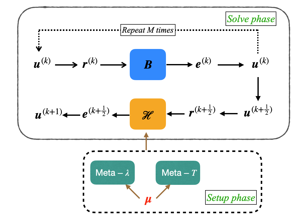
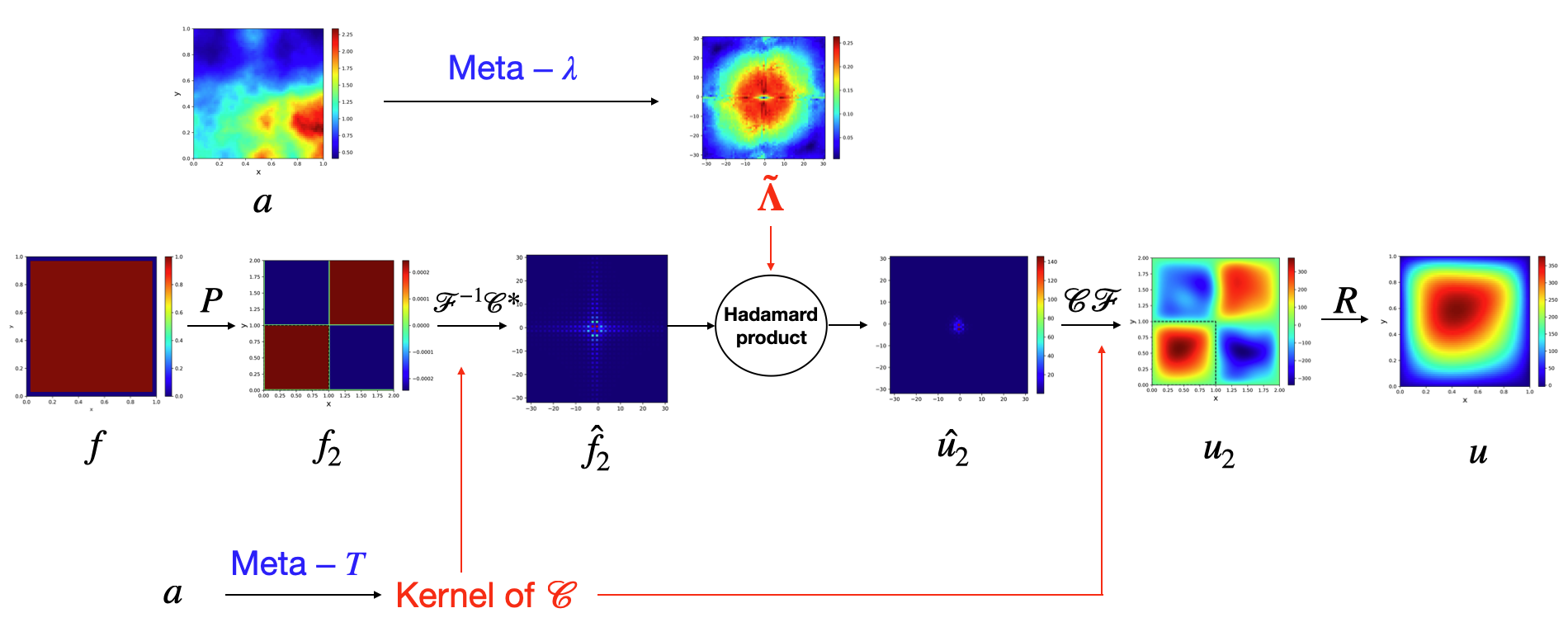
Since most existing neural operators have these properties [16], we employ the commonly used Fourier neural operator (FNO) [55] and UNet as Meta and Meta. The schematic diagram of FNS is illustrated in Figure 1, which consists of two stages: setup phase and solve phase. During the setup phase, two meta subnets are used to give the parameters required for the . The specific operation of will be detailed in the subsequent section. The meta subnets incorporate the nonlinear activation function to improve their expressive ability, which does not break the linearity of with respect to its input. The linearity of with scale-equivalent property can give the correction error associated with residuals with different orders of magnitudes, thereby mitigating the issue of poor generalization in neural networks for data exceeding two orders of magnitude [56]. The computational complexity of a single-step iteration during the solve phase is .
Remark 2
In fact, we did not extensively explore the architecture of the meta network. Hyper nets in [22, 40], encoder nets in [57, 44], and branch nets in [36, 47] play similar roles but utilize different network structures. By tailoring the meta structure to the specific characteristics of the problem, one might achieve better results than those presented in the next section.
Returing to the question raised at the end of the previous section, the improved in (34) overcomes spectral bias by learning the corresponding eigenvalues and eigenvectors in the frequency domain with the help of additional meta subnets. This provides a structural advantage over the used in existing DL-HIM. Next, we construct appropriate training data and loss functions for learning FNS to meet the requirements of Theorem 1.
3.1 Training data and loss function
Some DL-HIM [36, 38, 47, 39] train separately using supervised learning with a loss function of the form
Here, the data pairs are generated by solving PDEs. This approach is not only computationally expensive but also contain all frequency error components without accounting for the role of . In training neural solvers, one common approach is to sample from a certain distribution, such as , and obtain by computing . However, this method results in , which is biased toward the dominant eigen-subspace of . Consequently, this can lead to poor performance of the neural solver when dealing with inputs that are close to the bottom eigen-subspace [49].
The loss function we employed is the relative residual
| (45) |
where is the solution vector obtained after applying (4) times, starting from a zero initial guess, and is sampled from . This approach ensures that the input to follows the distribution . When is selected as a simple preconditioner, such as the diagonal Jacobi preconditioner, this distribution tends to be skewed toward the dominant eigen-subspace of , which presents challenges for to effectively handle. Moreover, instead of constructing data for each fixed , we generate various matrices from the discretized PPDE (5). Since the discrete systems considered in this paper are based on structured grids, and all matrix-vector multiplications can be performed using convolution, there is no need to store the sparse matrix . Our training data consists of tuples .
4 Numerical experiments
In this section, we evaluate the performance of FNS on discrete systems derived from several types of PPDE. These systems vary in their algebraic properties and the challenges they present, including:
-
(1)
Random diffusion equation: Poisson-like elliptic problem, non-symmetric, positive definite.
-
(2)
Anisotropic diffusion equation: Multiscale, symmetric positive definite.
-
(3)
Convection-diffusion equation: Non-symmetric, positive definite.
-
(4)
Jumping diffusion equation: Multiscale with different scales at different grid points, non-symmetric, positive definite.
We implement FNS using the PyTorch deep learning framework [58] and conduct numerical experiments on an Nvidia A100-SXM4-80GB GPU. The code will be made available upon publication.
4.1 Random diffusion equations
Consider the following two-dimensional (2D) random diffusion equation
| (46) | ||||
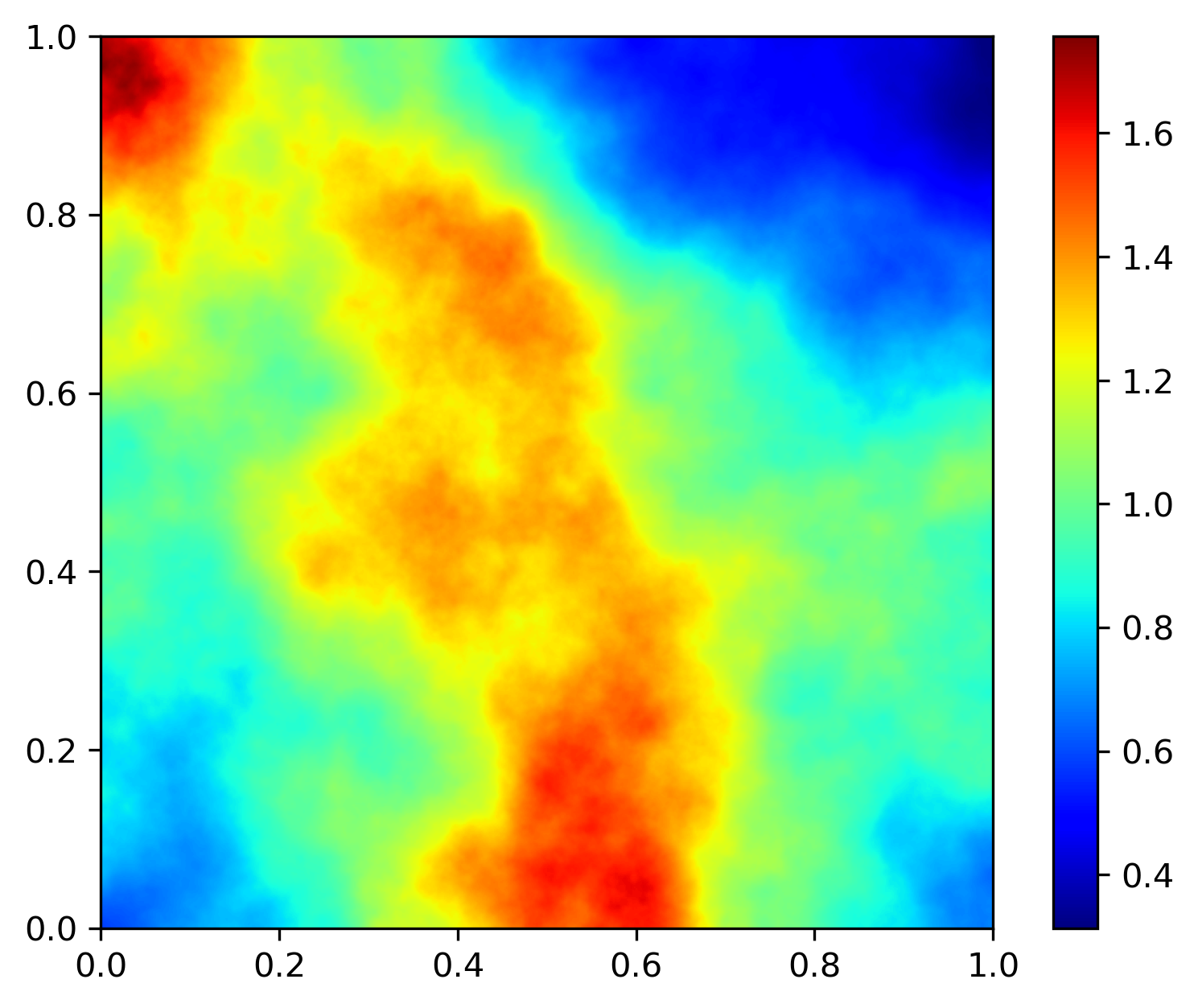
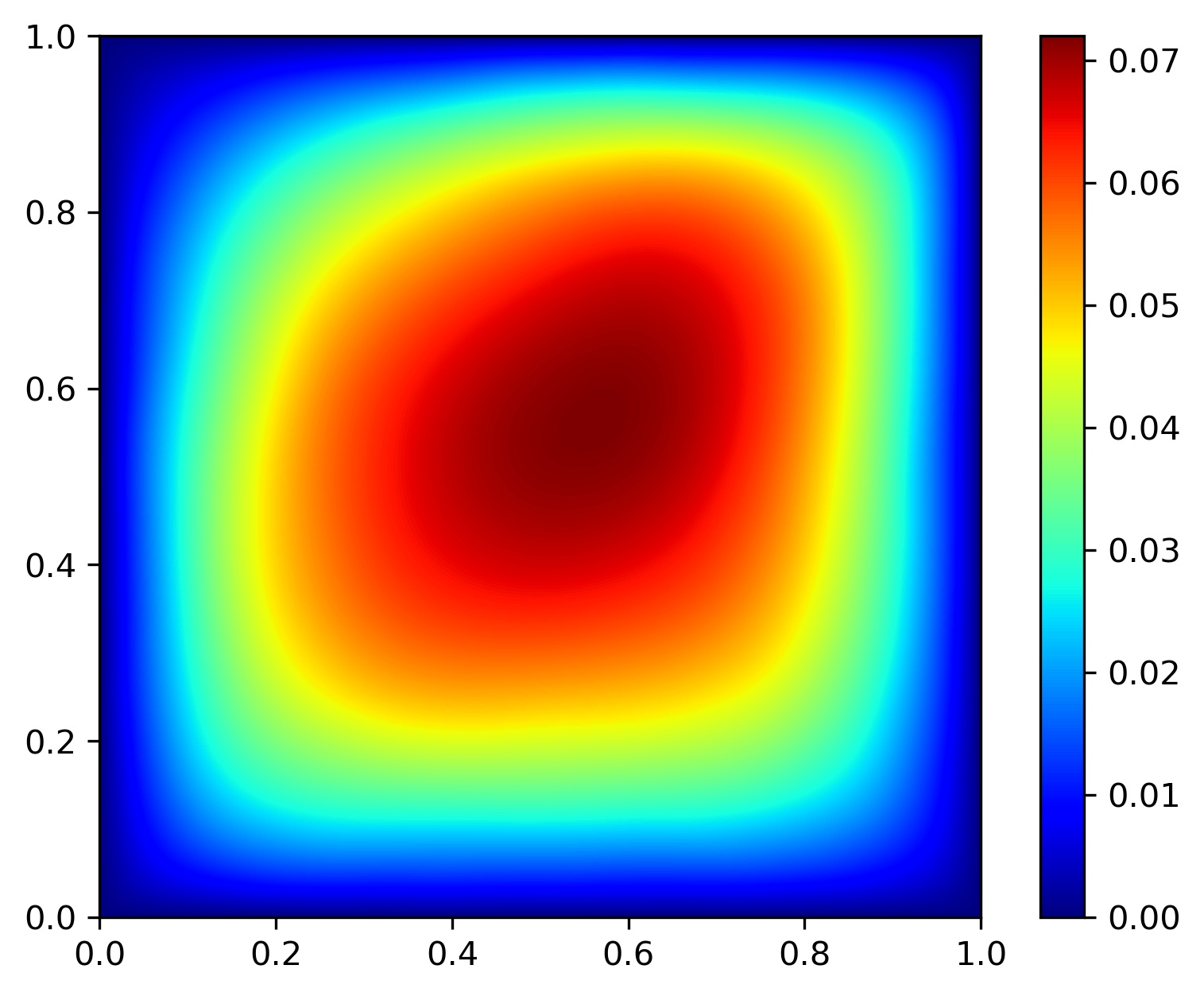
where the diffusion coefficient , and is the exponential function [55]. Figure 2(a) shows an example of , and Figure 2(b) shows the corresponding numerical solution when . This equation models not only diffusion but also steady-state Darcy flow in porous media, steady-state heat conduction, and similar processes.
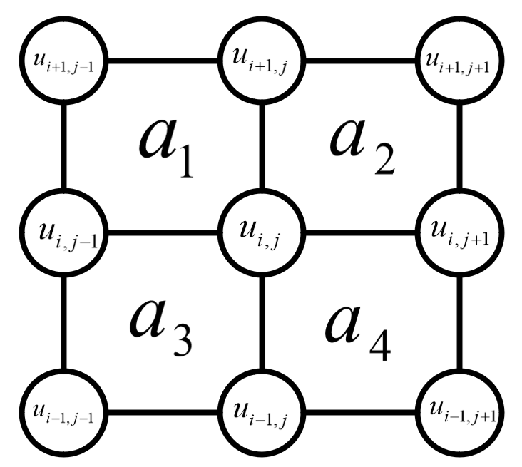
We use bilinear FEM on squares with sides of length . The discrete equation at an interior mesh point with indices is
| (47) | ||||
where and are constant random coefficients corresponding to the four neighboring elements of index , as shown in Figure 2(c).
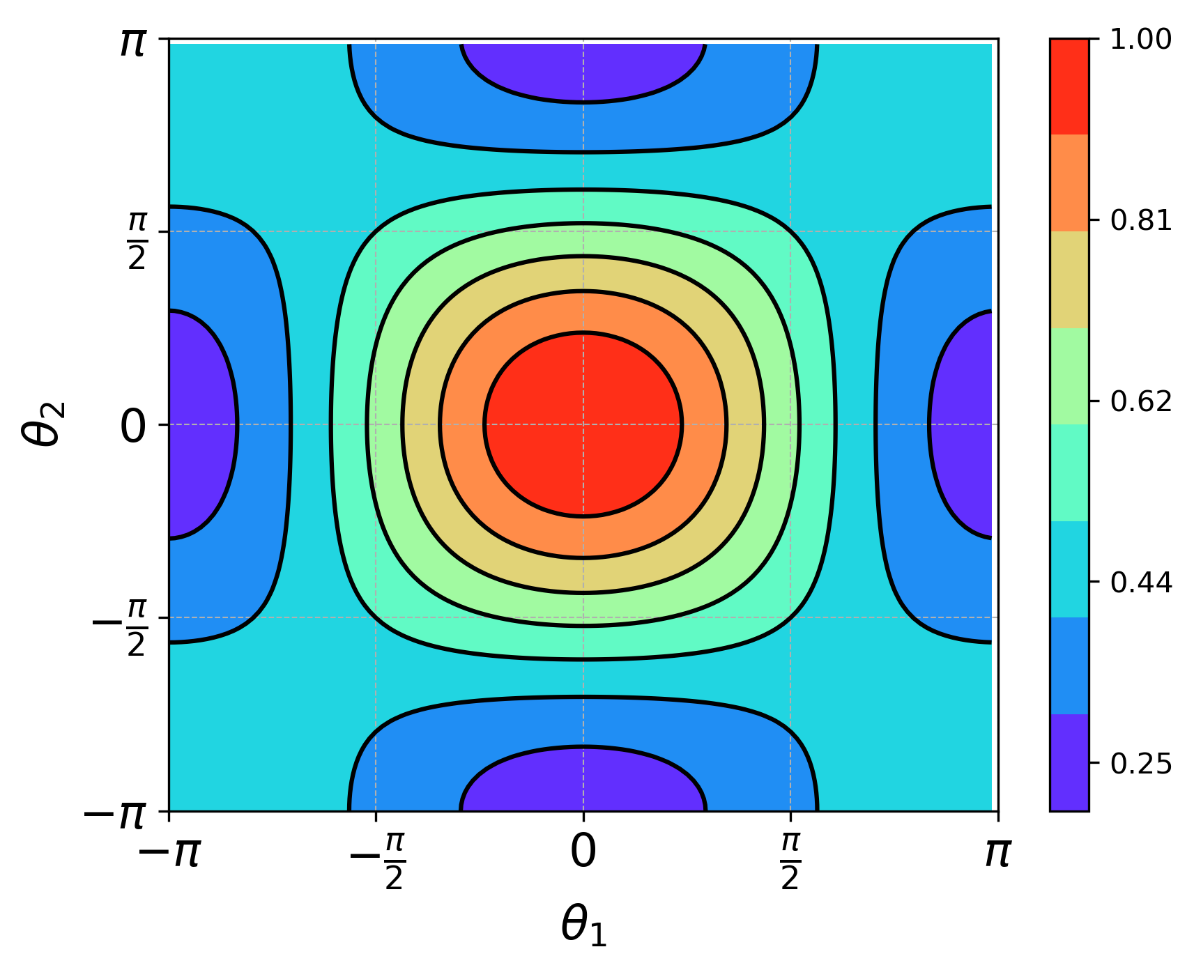
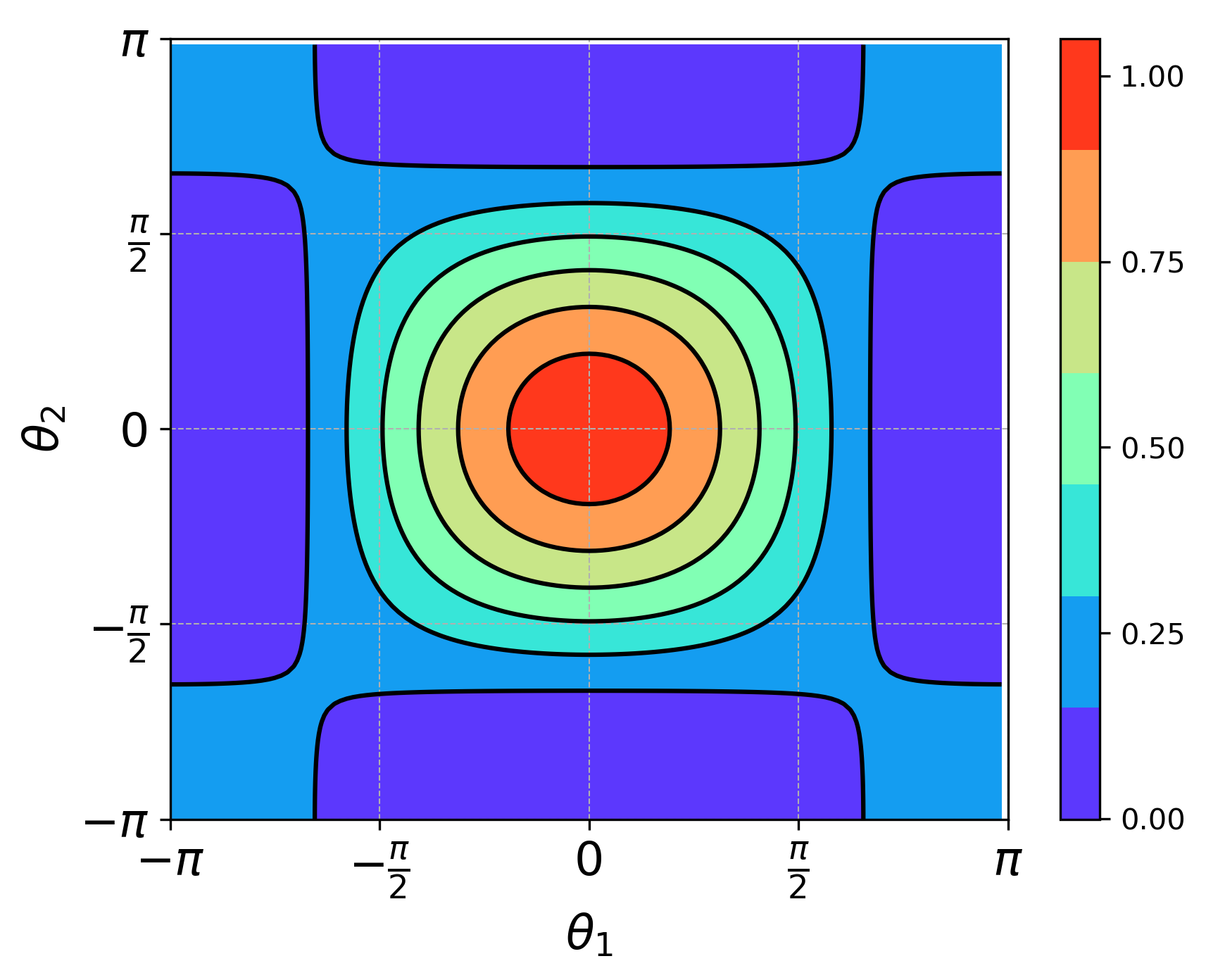
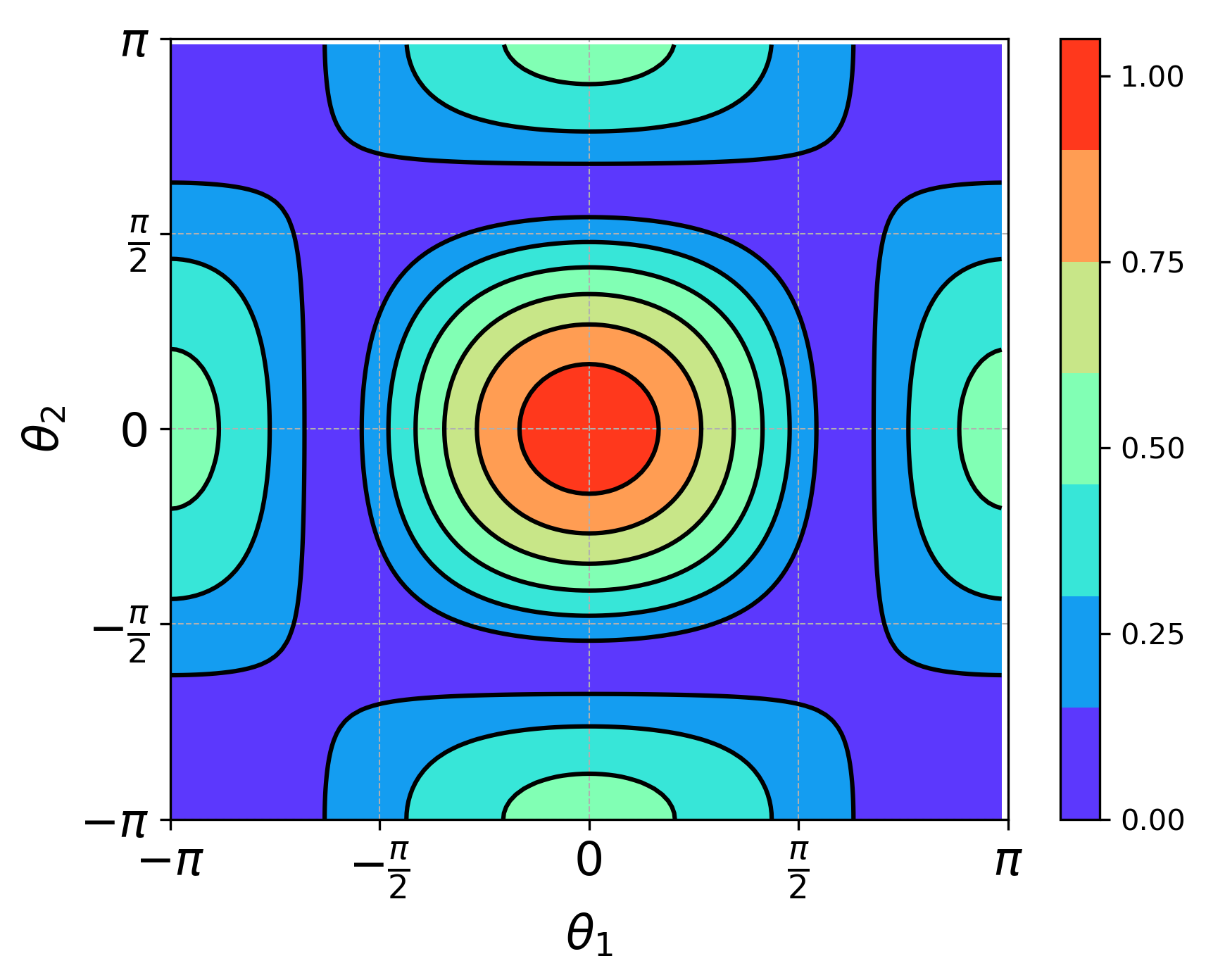
Selecting as the damped Jacobi method, we use non-standard LFA [51] to evaluate its compressibility for error components with different frequencies. Figure 3 shows the modulus of the formal eigenvalue of the damped Jacobi method (abbreviated as the Jacobi symbol) with different weights when solving the discrete system corresponding to depicted in Figure 2(a). It can be observed that the damped Jacobi method exhibits poor compressibility for error components with frequencies in , regardless of the value of . Let and , it can be found that when , the damped Jacobi method achieves the best compressibility for the error components with frequencies in . Therefore, we choose as the damped Jacobi method with , which can meet Assumption 2.1.
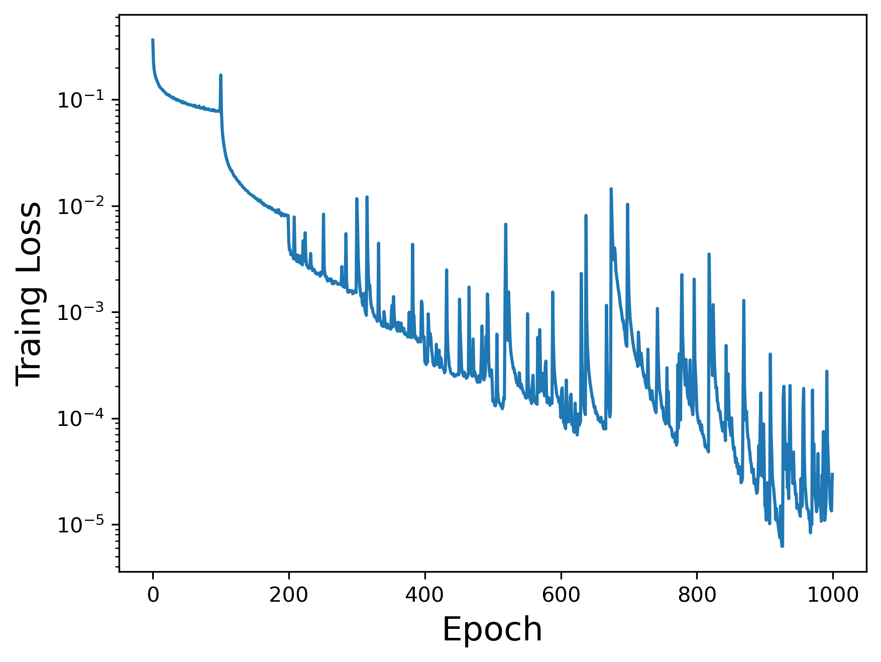
Next, we train FNS to ensure satisfies Assumption 3.1 as much as possible. For this problem, we aim for the trained FNS to generalize well for both and . According to previous analysis, the asymptotic convergence rate of FNS is independent of RHS (as we will verify below), so is the only parameter of interest, corresponding to in PPDE (5). We generate 10,000 random diffusion coefficients with scale and sample a random RHS for each parameter . We employ the loss function (45) for unsupervised training, utilize the Adam optimizer with an initial learning rate of and a learning rate schedule that halves the learning rate every 100 epochs. Additionally, we increase by one every 100 epochs and set . The training loss is depicted in Figure 4.
Now we test the trained FNS. Figure 5 illustrates the calculation flow of when it receives an input pair . It can be observed that the given by Meta- is large in and small in , which aligns with our expectations. By inputting the RHS into , we obtain an initial value close to the reference solution, indicating that effectively captures the low-frequency components of the solution.
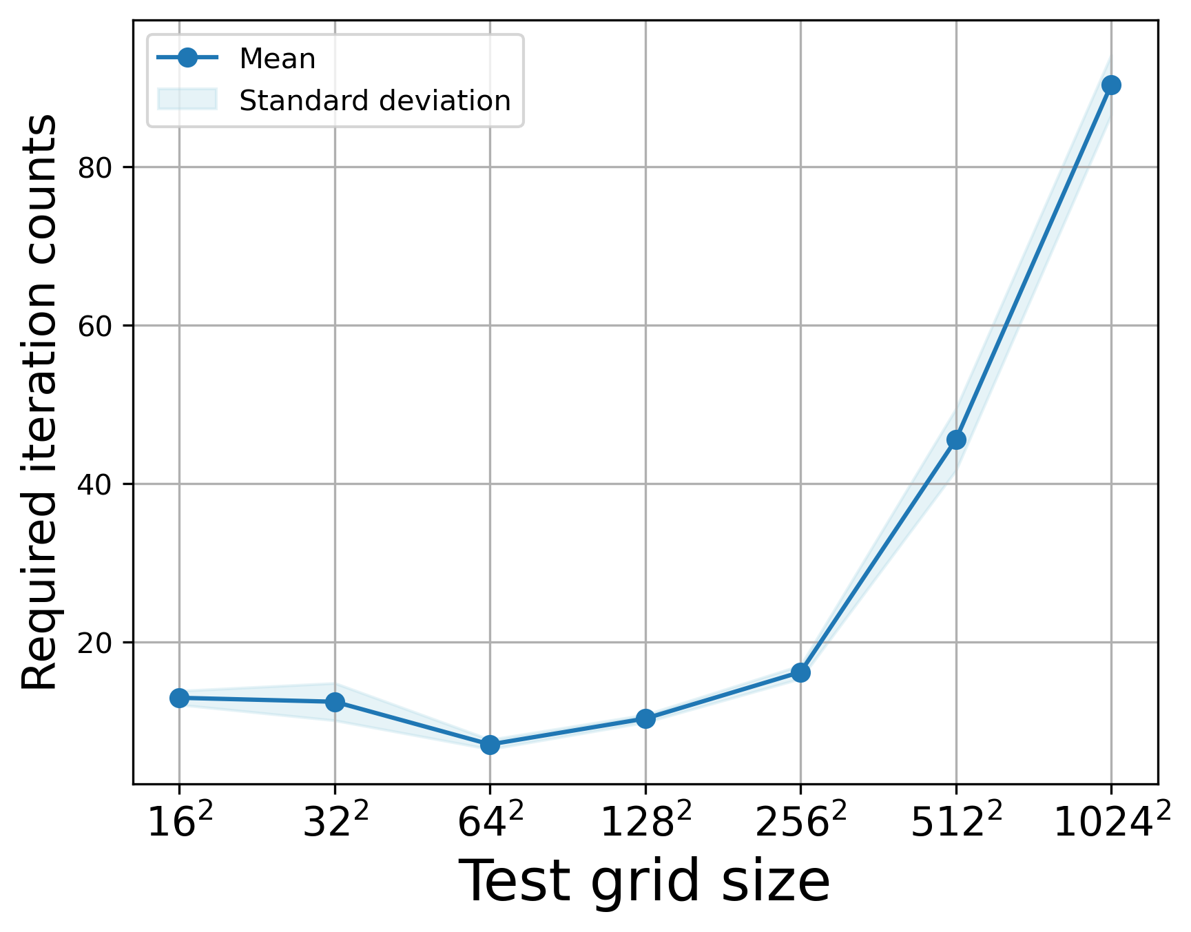
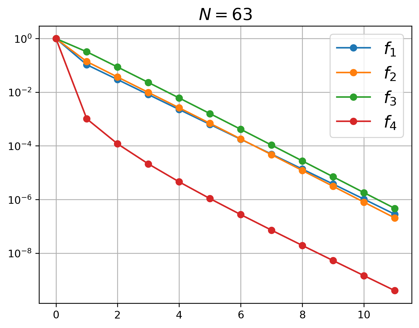
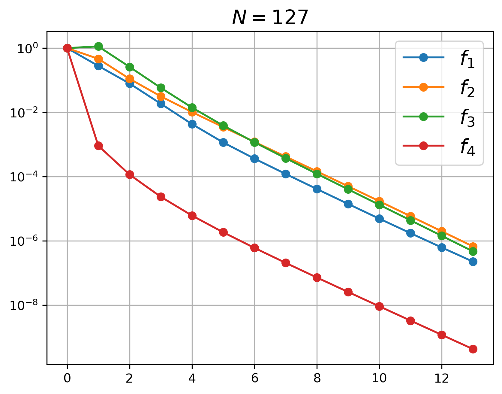
Then we test the convergence speed of FNS on different scales. For each scale, we sample 10 different coefficients and fix . Figure 6 illustrates the mean and standard deviation of the FNS iteration counts required to achieve a relative residual of less than . The results indicate that when , the convergence rate of FNS is almost independent of the grid size and the coefficients , which aligns with our analysis. However, as the scale increases further, the number of required iterations grows linearly with the scale.
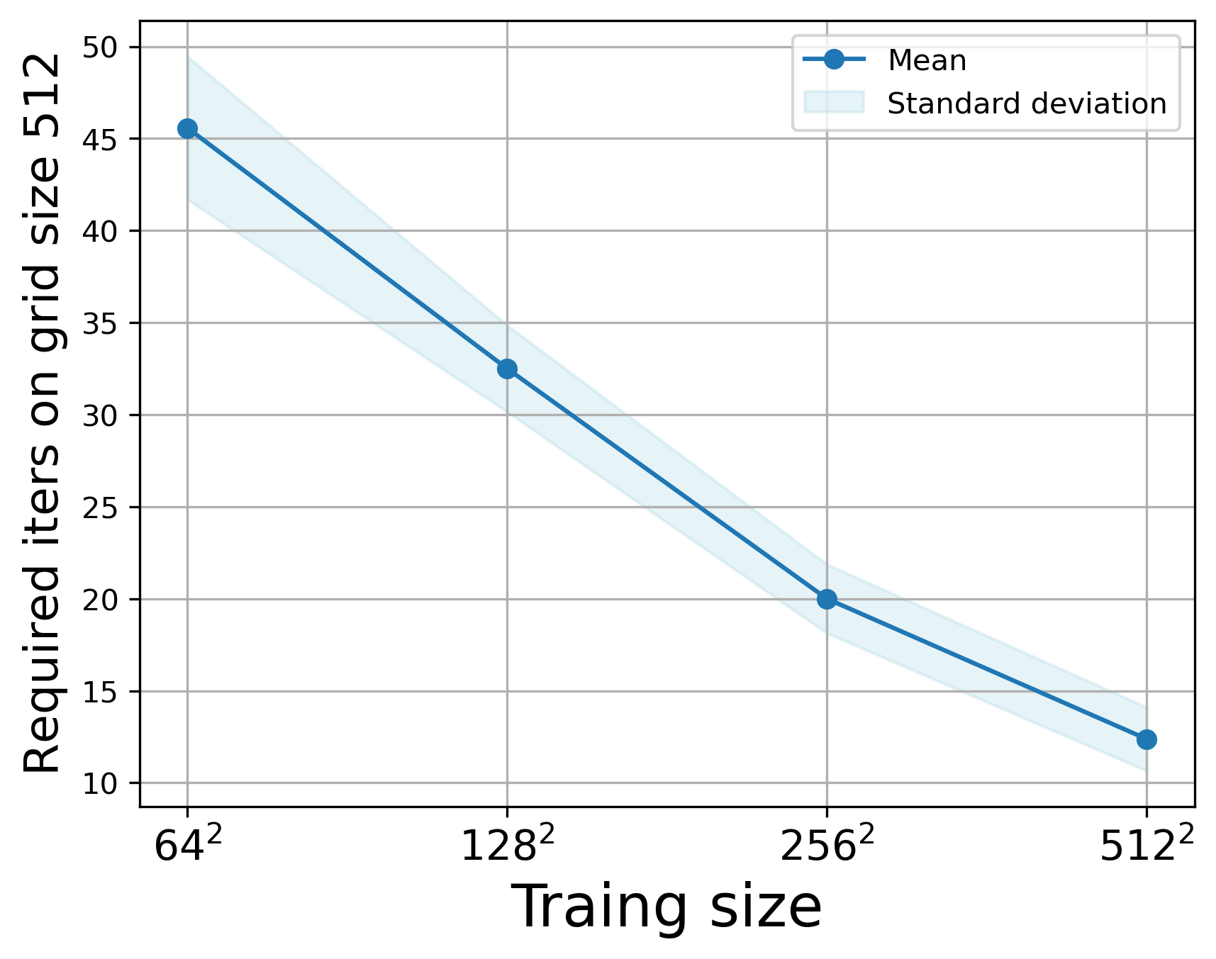
To address this issue, we keep the parameter counts of the meta subnets invariant while increasing the training data. According to the neural scaling law, as the size of the training data increases, the performance of FNS improves accordingly. Figure 6 presents the FNS iteration counts trained on different grid sizes but tested on a scale of . As the training data size increases, FNS performance improves, indicating that a fully trained FNS better satisfies Assumption 3.1, making the number of iterations independent of the scale. However, training with large datasets is computationally expensive, so enhancing the generalization capability of FNS trained on smaller scales remains a challenge to address in the near future.
Remark 3 (Generalization of FNS on different RHS)
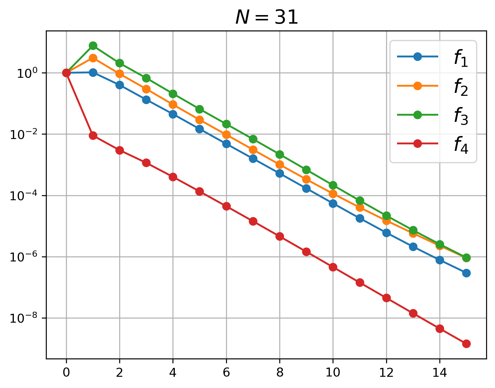
When using iterative methods, we often start with a zero initial guess. In this case, the frequencies present in the initial error are determined by , and those in the initial residual are determined by . Below, we compare the behavior of FNS when solving four different RHS:
-
(1)
Single frequency function:
-
(2)
Gaussian function:
-
(3)
Constant function:
-
(4)
Random function:
Figure 7 shows the comparison results. It can be seen that although the error reduction of the first step differs due to the different RHS, the asymptotic convergence rate remains almost the same.
4.2 Anisotropic diffusion equations
Consider the following 2D anisotropic diffusion equation
| (48) |
where the diffusion coefficient is a constant matrix
| (49) |
is the anisotropic strength, and is the anisotropic direction, . Using bilinear FEM on a uniform rectangular mesh with size , the resulting stencil is
| (50) |
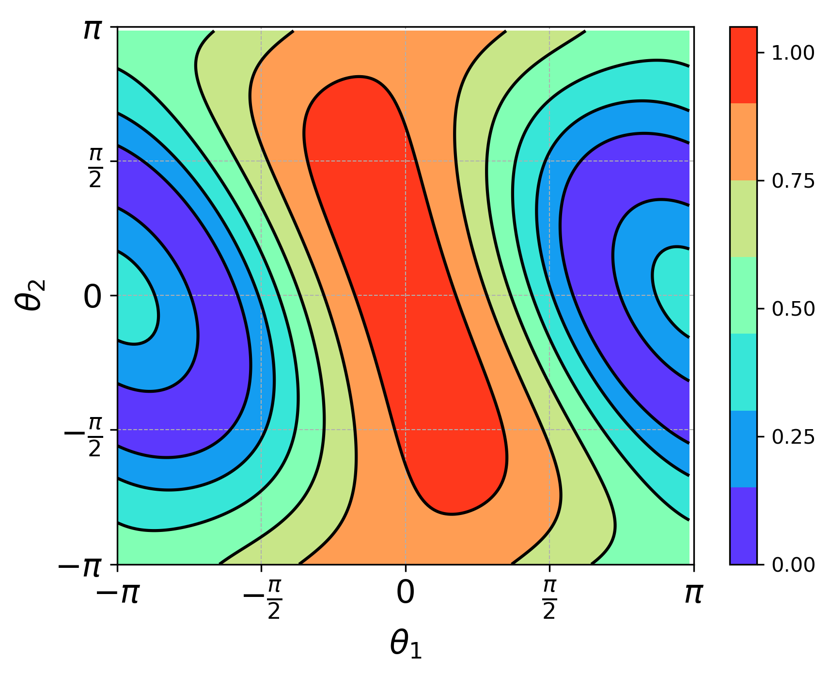
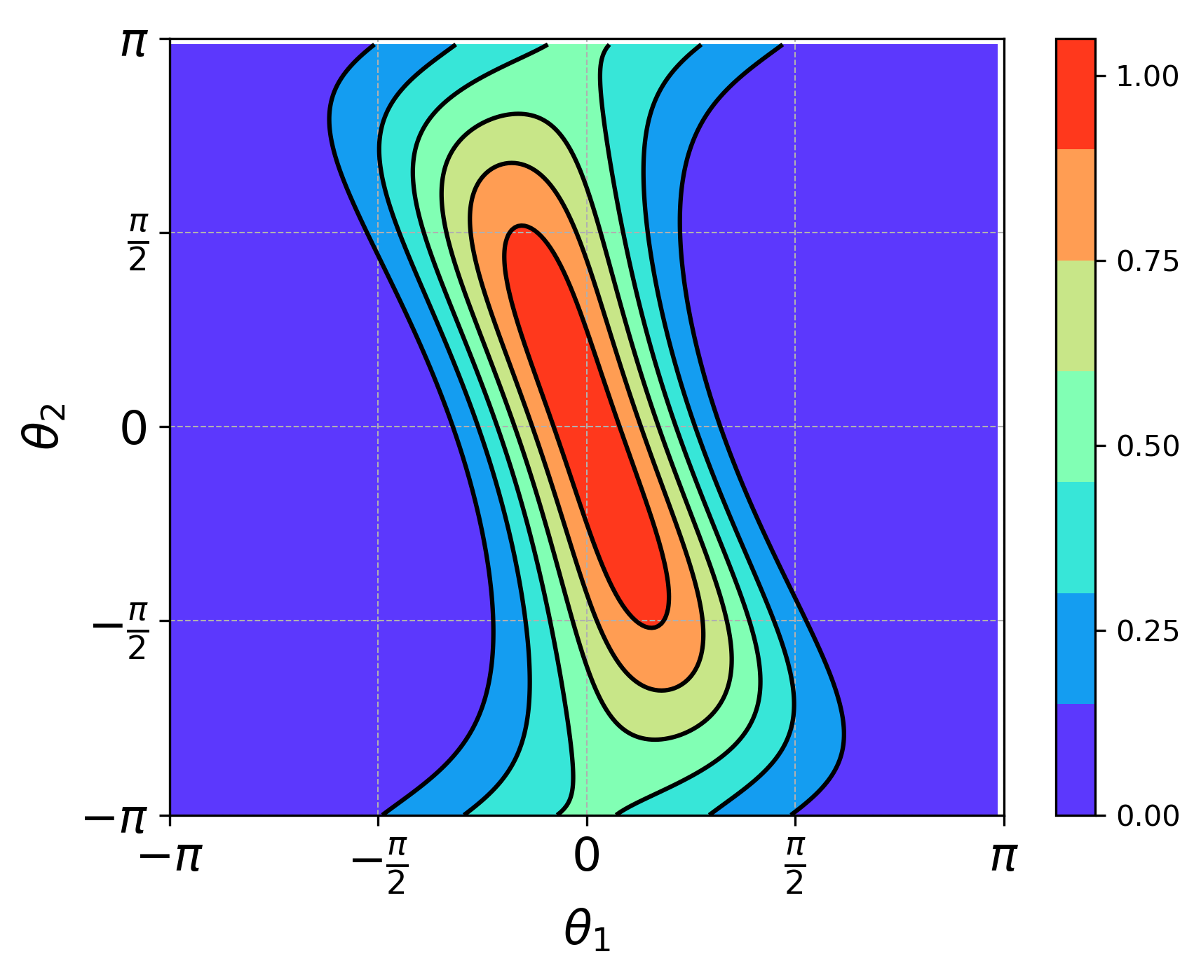
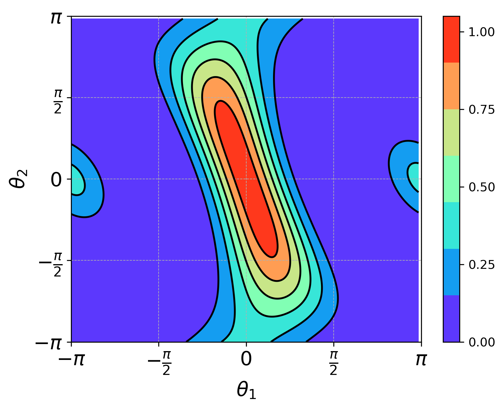
Selecting as the damped Jacobi method, Figure 8 shows the Jacobi symbol when solving the anisotropic discrete system corresponding to , . It can be seen that when the damped Jacobi method uses and , error components with frequencies along the anisotropic direction are difficult to eliminate. We denote the frequency interval along the anisotropic direction as and . To enhance the compressibility of error components with frequencies in , we increase to 5. Figure 8(b) shows the distribution of the corresponding symbol, which has improved a lot. The reason for using is that remains connected under this weight. If is further increased, such as to , will appear in other parts of the domain, which will increase the learning difficulty for .
Next, we train FNS to ensure that satisfies Assumption 2.2. Corresponding to PPDE (5), in this example. We sample 500 sets of parameters in the parameter interval according to the uniform distribution. For each parameter , we sample 20 RHS , and use the loss function (45) for unsupervised training. The hyperparameters used during training are the same as those used in the random diffusion equations.
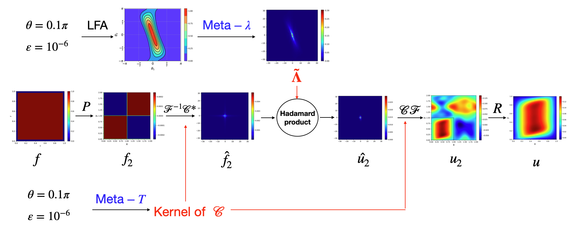
Once trained, we test the performance of FNS on newly selected parameters and different scales. Figure 9 shows the calculation flow of when receiving specific parameters and . The difference compared to the random diffusion equation is that, instead of directly inputting the parameter into the Meta-, we use the Jacobi symbol obtained by LFA as input. This is because the symbol contains more intuitive information than and is easier to learn. From Figure 9, it can be seen that the given by Meta- is large in but small in , which is consistent with our expectations.
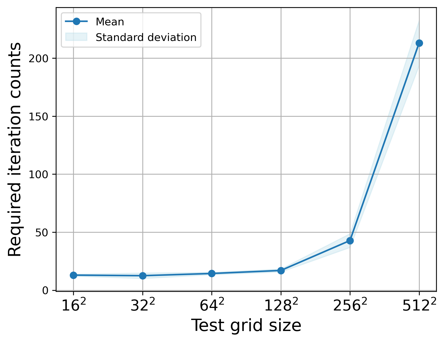
Similarly, we test the required iteration counts of FNS when solving different anisotropic equations with various parameters on different mesh scales . For each scale, we sample 10 different and calculate the mean and standard deviation of iteration counts. Since smaller leads to a stronger multi-scale property of the discrete system, we sample the test parameters within . Figure 10 shows the results. It can be seen that when , the FNS iteration counts are almost invariant with and , but they increase significantly beyond . We believe this may be addressed by increasing the amount of large-scale training data, increasing the parameters of meta subnets, and using more powerful optimization algorithms.
4.3 Convection-diffusion equations
Consider the following 2D convection-diffusion equation
| (51) | ||||
where is a viscosity parameter, and is the flow velocity, assumed to be incompressible (). We are interested in the convection-dominated case, i.e. , . In this setting, the solution typically has steep gradients in some parts of the domain. If we apply the usual Galerkin FEM, a sharply oscillating solution will be obtained. To avoid this problem, we use the streamline diffusion FEM, which finds such that
| (52) | ||||
where is a user-chosen non-negative stabilization parameter, which plays a key role in the accuracy of the numerical solution. As shown in [59], a good choice of is
| (53) |
where is the element Péclet number. In the following, we consider steady flow and use bilinear finite element on a uniform grid with spacing . The corresponding stencil is given by
| (54) | ||||
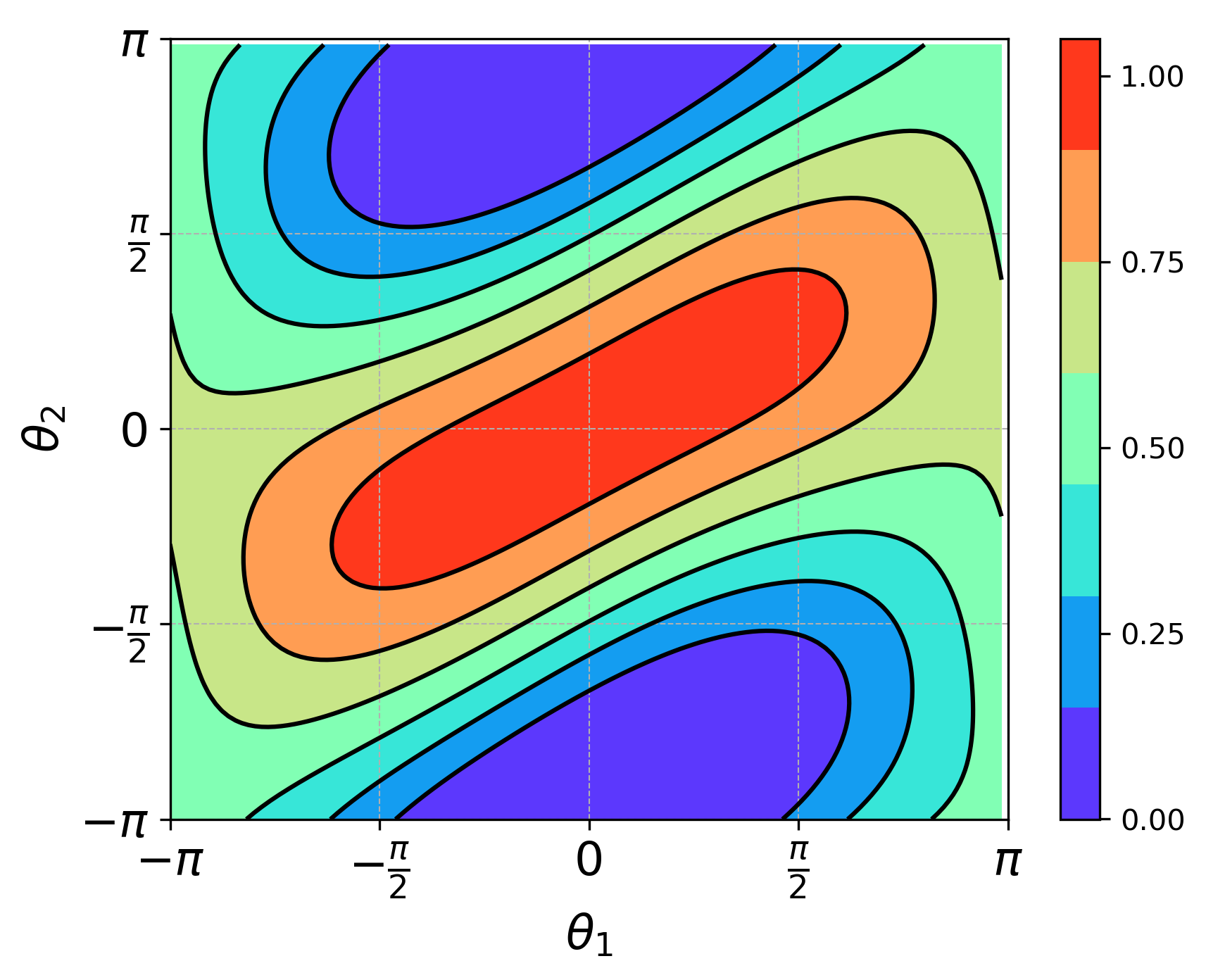
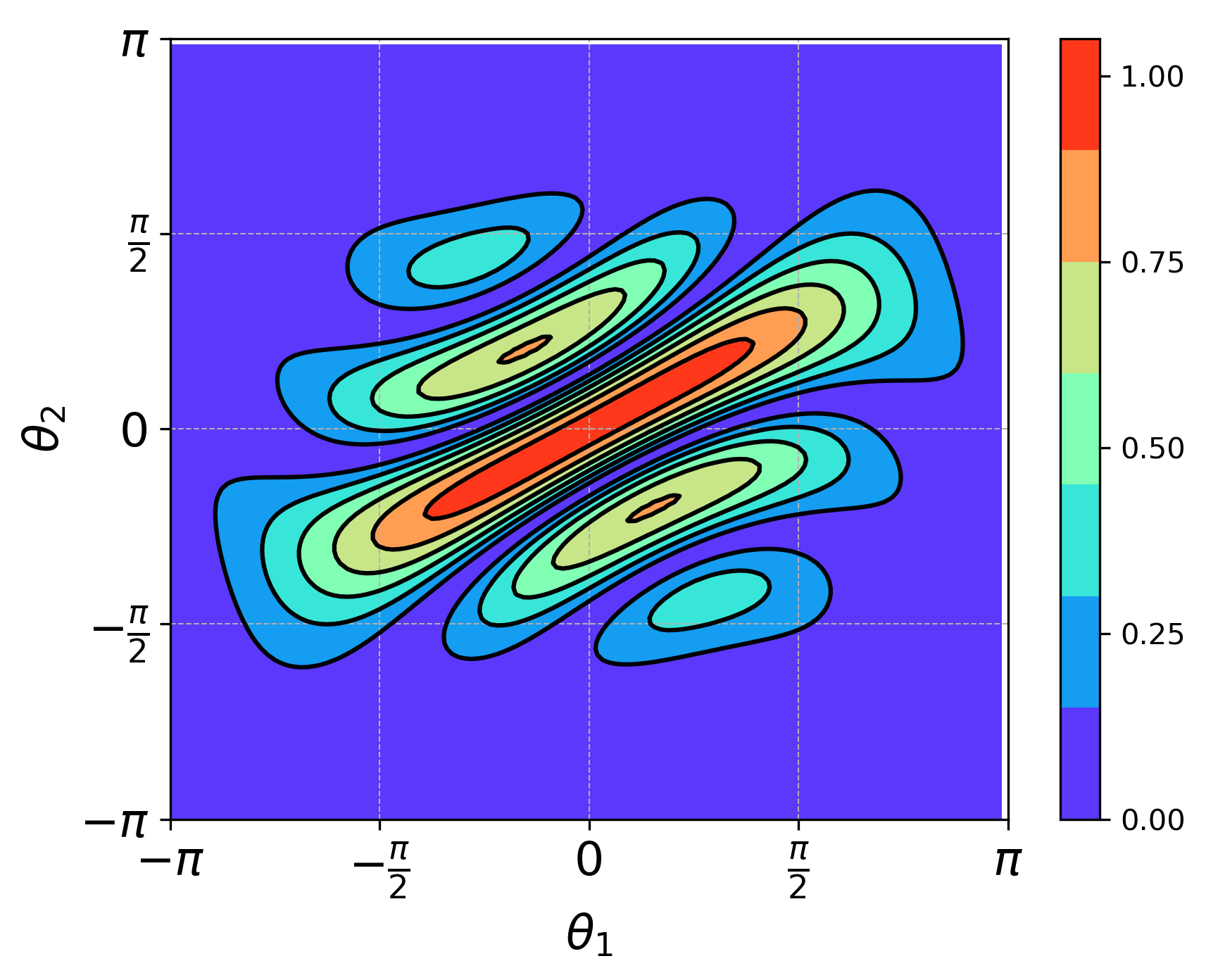
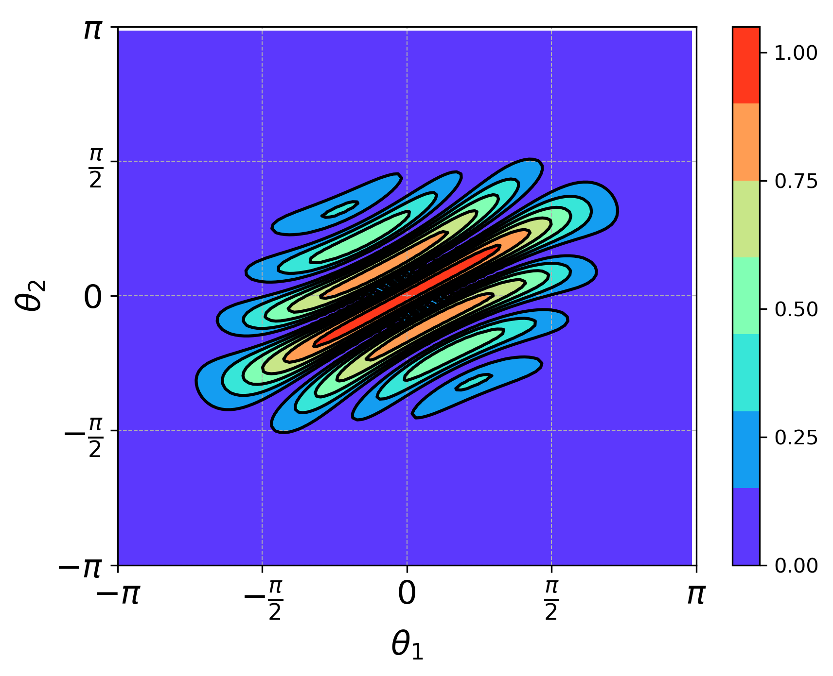
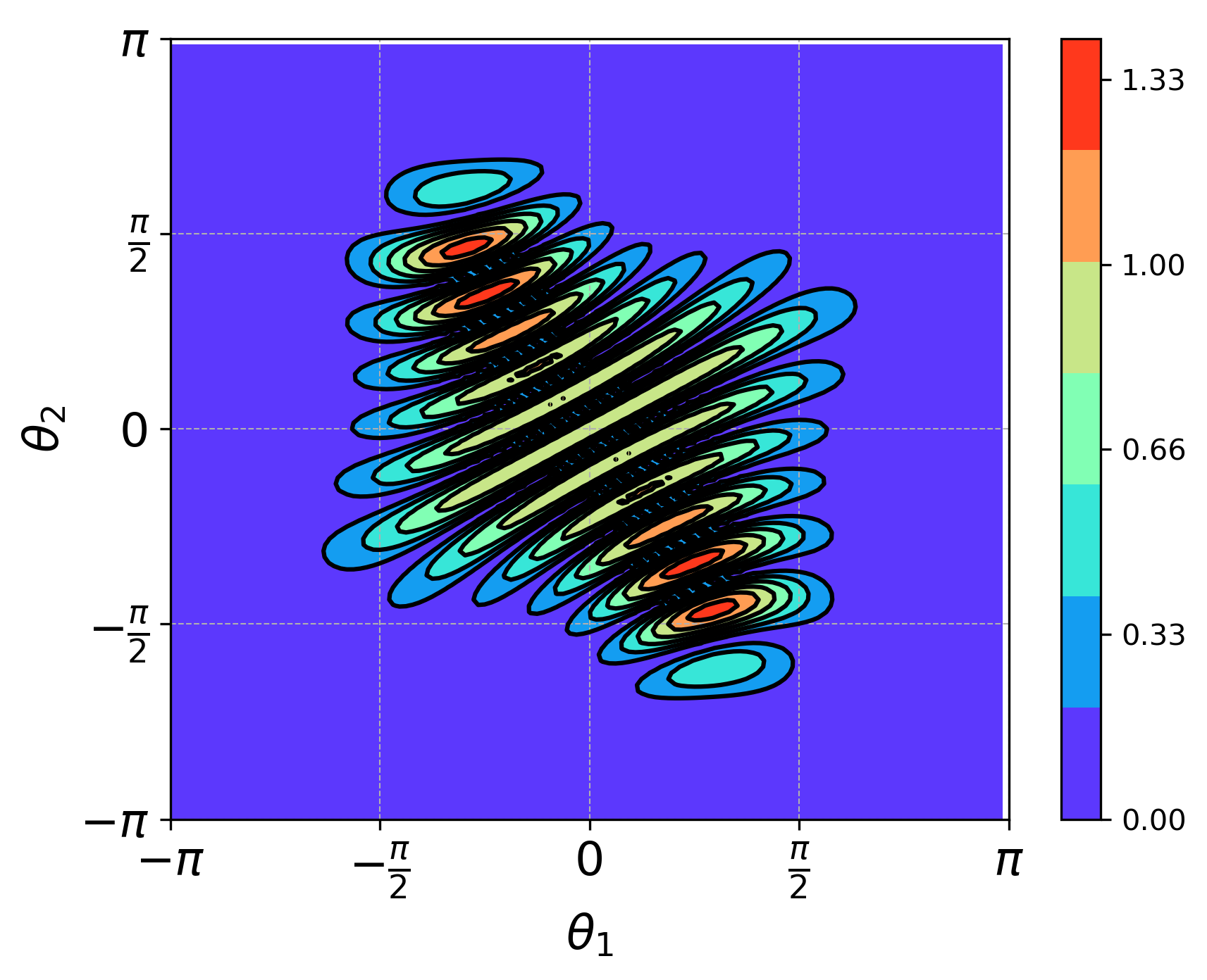
Selecting as the damped Jacobi method, we estimate its compressibility for error components with different frequencies using LFA. Figure 11 shows the Jacobi symbol for different weights and iteration counts when applied to the discrete system corresponding to , , and . The first three plots show that when , the damped Jacobi method has a better smoothing effect for error components with frequencies except along the streamline direction as increases, which means Assumption 2.1 can be met. However, when increases, such as to , the damped Jacobi method not only fails to achieve a better smoothing effect but also amplifies the error components with certain frequencies. Therefore, we take and .
Next, we train FNS to make satisfy Assumption 3.1. Corresponding to the PPDE (5), the parameters of this problem are . We sample 100 sets of parameters as follows: and . Taking as the training size, we calculate the corresponding according to (53) and then obtain the corresponding stencil (54). For each set of parameters , we randomly generate 100 RHS according to the standard normal distribution, obtaining a total of 10,000 training data pairs.
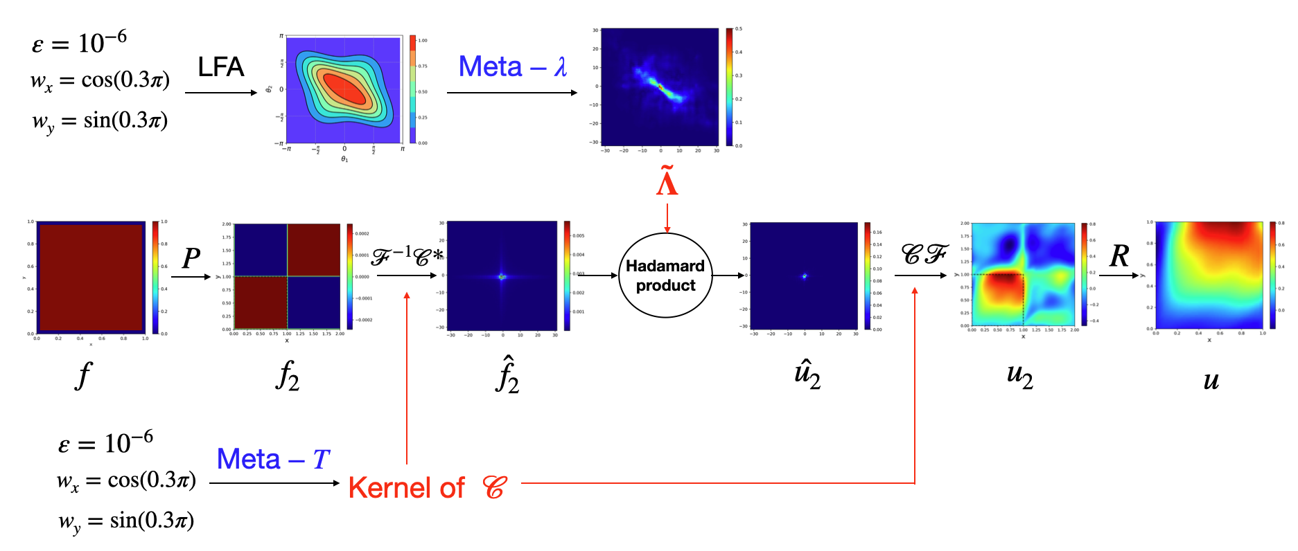
After training, we test the performance of FNS. Figure 12 shows the calculation flow of when it receives a pair of . Since the smoothing effect of on the convection-diffusion equation is similar to that of the anisotropic diffusion equation, we also first perform LFA on to obtain its symbol, and then input the symbol into the Meta-. From Figure 12, we can see that the given by Meta- is large in but small in , which is consistent with our expectations.
Table 1 shows the required iteration counts of FNS, which is trained on the scale but test on other scales. It can be seen that the convergence speed of FNS is weakly dependent on the grid size .
| 31 | 63 | 127 | 255 | 511 | |
|---|---|---|---|---|---|
| iters | 8 | 12 | 16 | 19 | 23 |
4.4 Jumping diffusion equations
Consider the 2D diffusion equation with jumping coefficients
| (55) |
where
The function is a high-contrast piecewise constant function that jumps across the interface
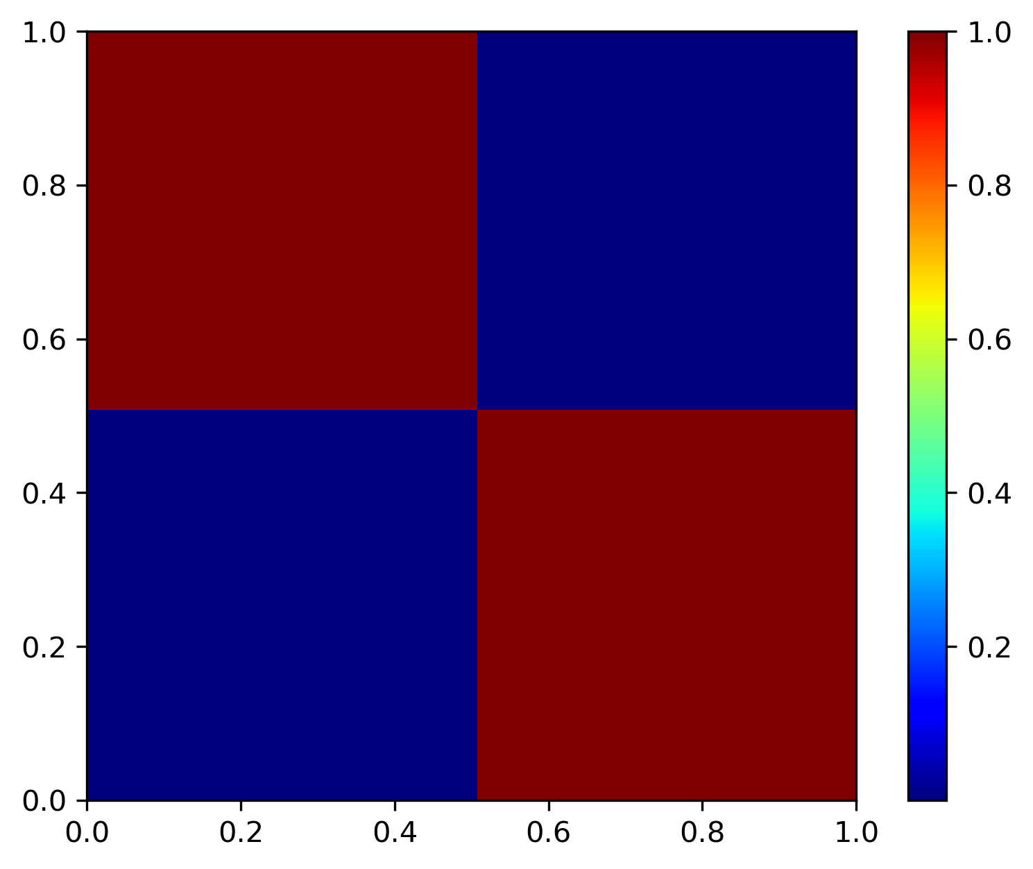
Figure 13(a)13(b) presents an example of the coefficients and the corresponding solution, where the red region represents and the blue region represents .
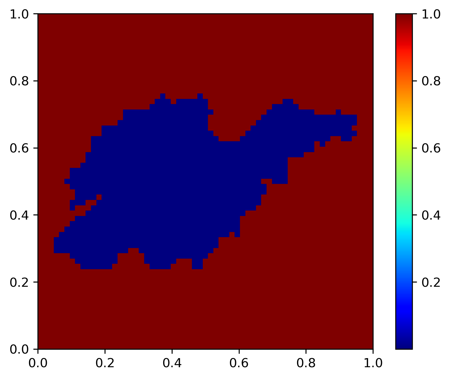
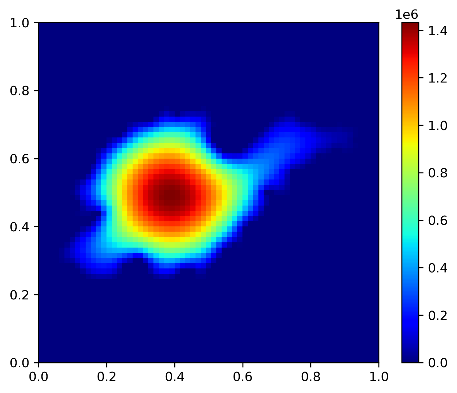
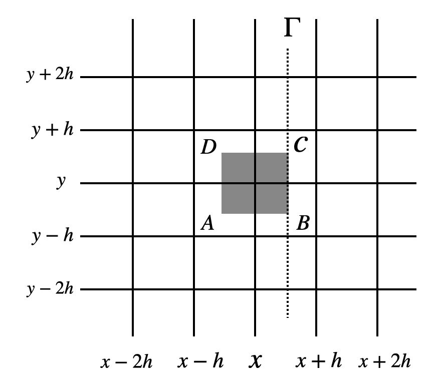
We employ the cell-centered finite volume discretization method [60]. To achieve this, a uniform grid with spacing is used, ensuring that the interface (dashed line) is fitted with the dual element (gray region), as illustrated in Figure 13(c). The resulting discrete system is
where the coefficients are
In comparison with the multi-scale property of anisotropic diffusion equations, the multi-scale property of this equation is also influenced by the node positions.
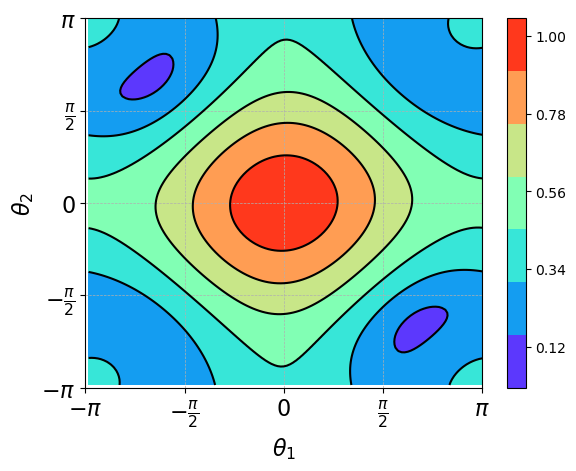
Consider as the damped Jacobi method. We calculate its compressibility for error components with different frequencies using non-standard LFA [52]. Figure 14 displays an example of and the Jacobi symbol with when solving corresponding discrete system. It can be seen that this is effective for eliminating high-frequency error components, while the compressibility for low-frequency errors is poor. Let and , then Assumption 2.1 is satisfied.
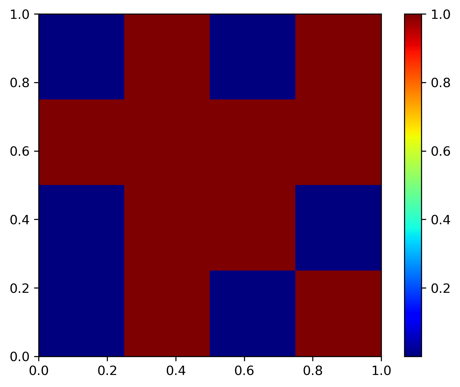
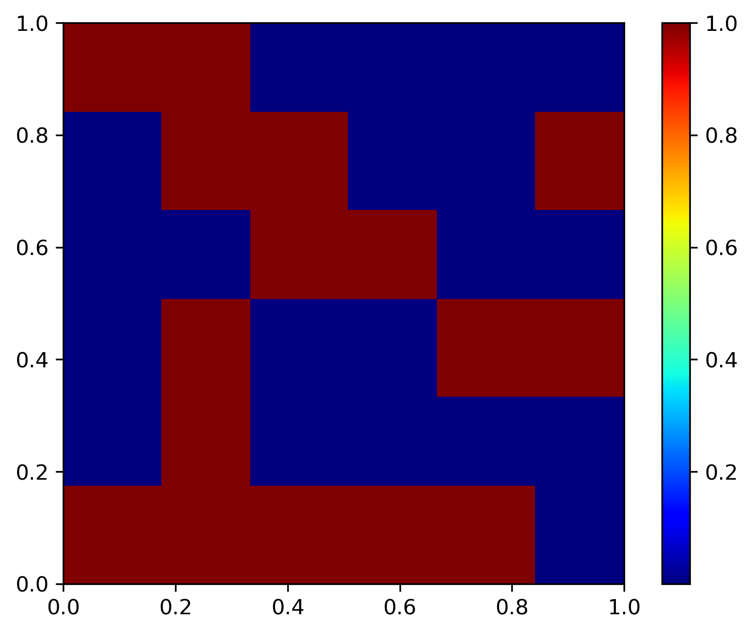
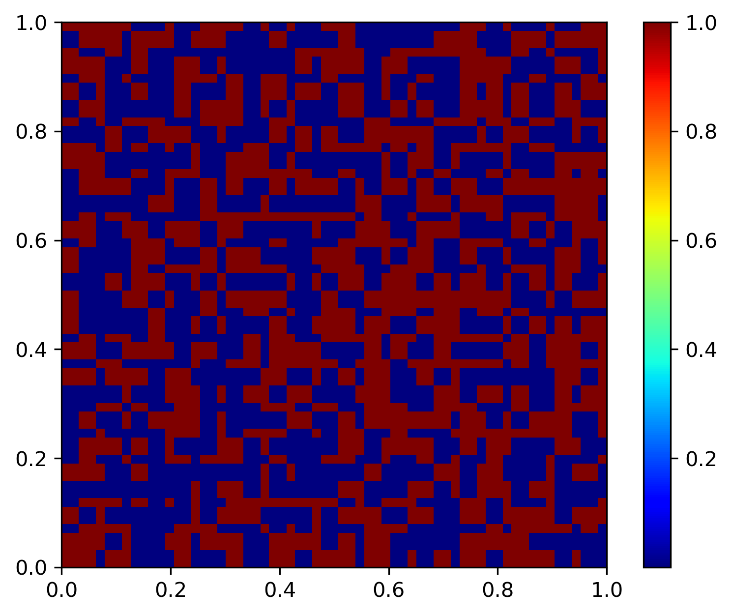
Next, we train FNS to ensure that satisfies Assumption 3.1. Corresponding to PPDE (5), in this example. We generate 10,000 different functions in the following way: split into checkerboard blocks, where the value of in each block is a constant, either or , with . For each , a random RHS is sampled, and unsupervised training is then performed using the loss function (45). The hyperparameters used during the training phase are the same as those used in the previous experiments.
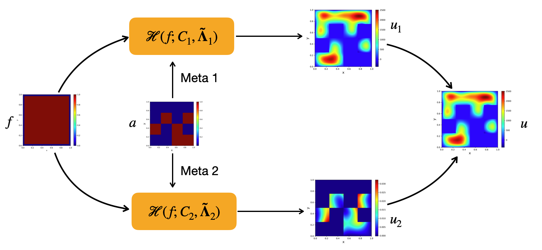
It is worth noting that due to the multi-scale property with respect to position, it is challenging to use one to learn the correction values for all components simultaneously. Therefore, we classify all nodes into two parts on a geometric level: nodes in form one category, and nodes in form another category. Correspondingly, two separate networks are used to learn the correction values for the first and second groups of nodes, respectively. Figure 15 shows the calculation flow of , where Meta 1 is used to learn corrections for nodes in (blue region), and Meta 2 is used to learn corrections for nodes in (red region). It can be seen that this geometric split naturally corresponds to the algebraic multi-resolution decomposition. This allows the network to learn the correction for nodes with the same order of magnitude only, making the learning process easier.
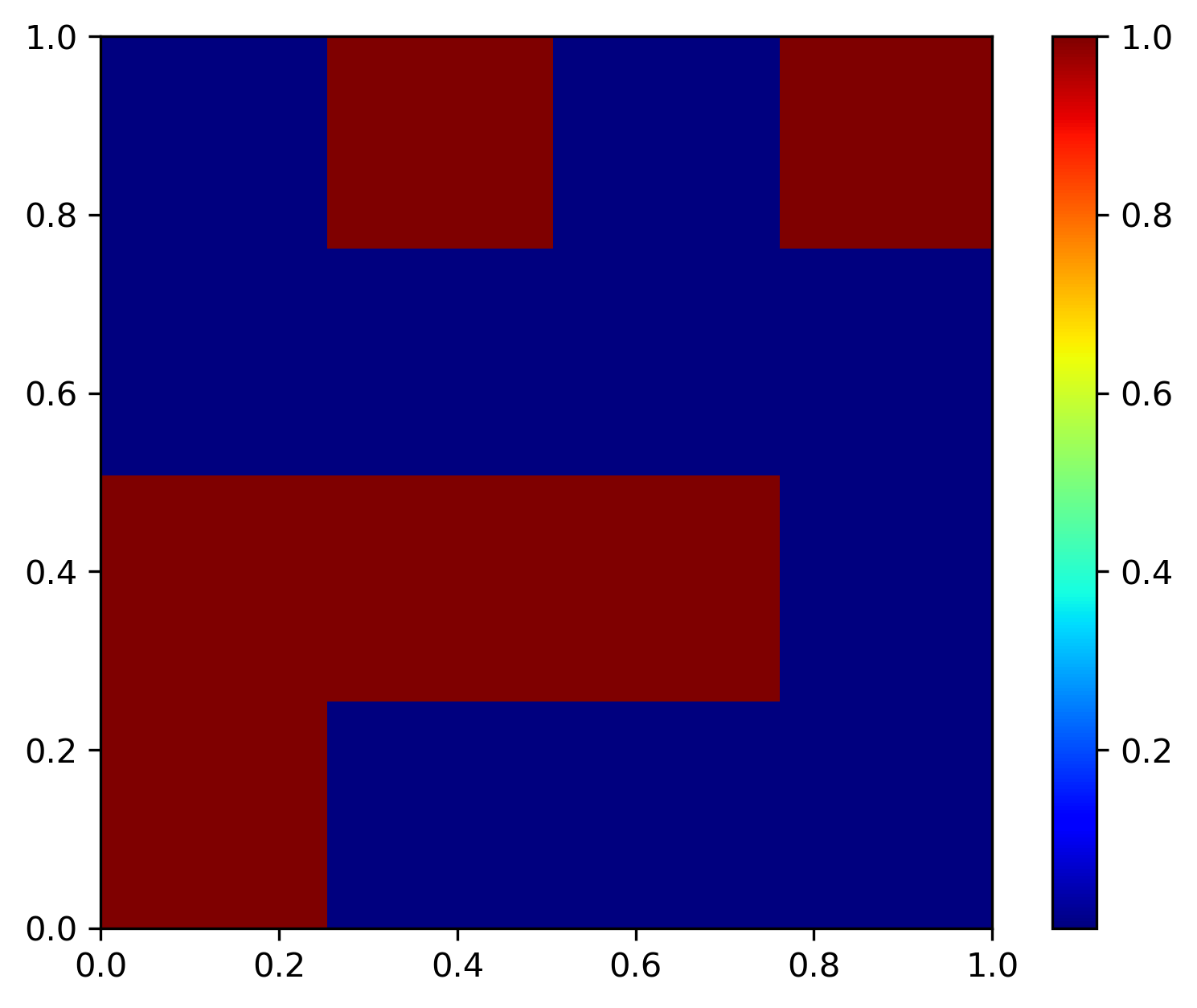
Next, we test the performance of FNS on varying scales. Table 2 shows the required iteration counts to solve the discrete system when the relative residual is less than for the coefficient shown in Figure 14(a) and . It can be seen that if FNS is only trained on the scale of , it has poor generalization to other scales. However, if FNS is trained on the testing scale, it can still learn suitable parameters on different scales, which significantly reducing the number of iterations. In the future, we aim to design better network architectures and use more powerful optimization algorithms to facilitate training.
| 15 | 31 | 63 | 127 | 255 | |
|---|---|---|---|---|---|
| Only trained on | 60 | 44 | 23 | 106 | 435 |
| Trained on the testing scale | 12 | 23 | 23 | 41 | 70 |
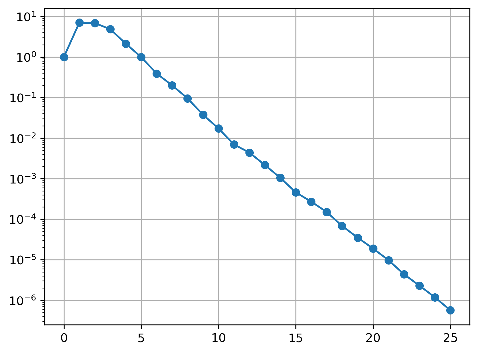
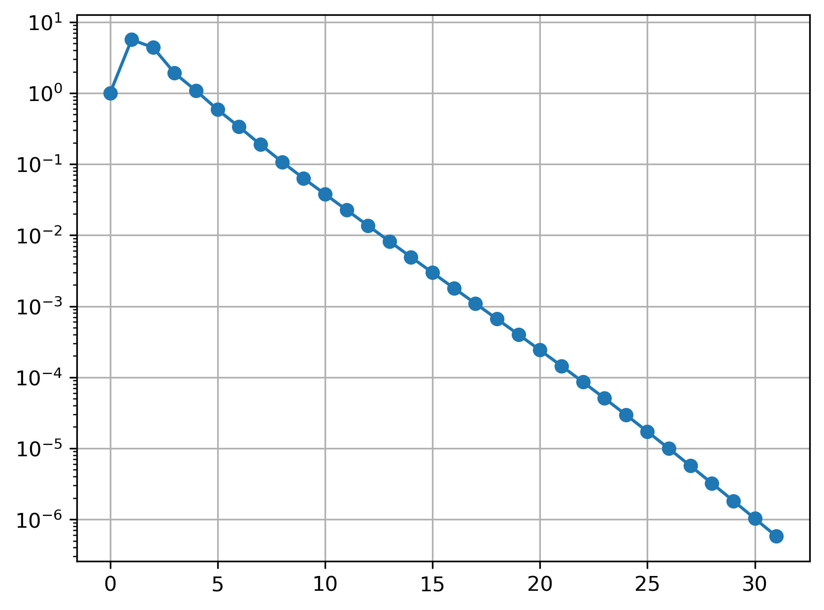
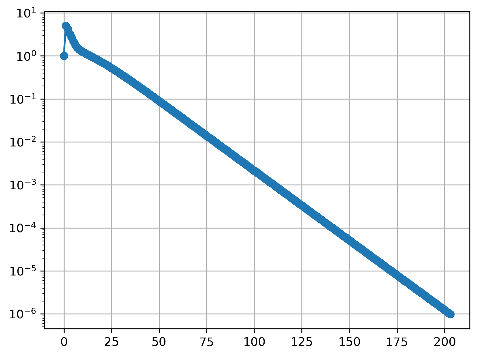
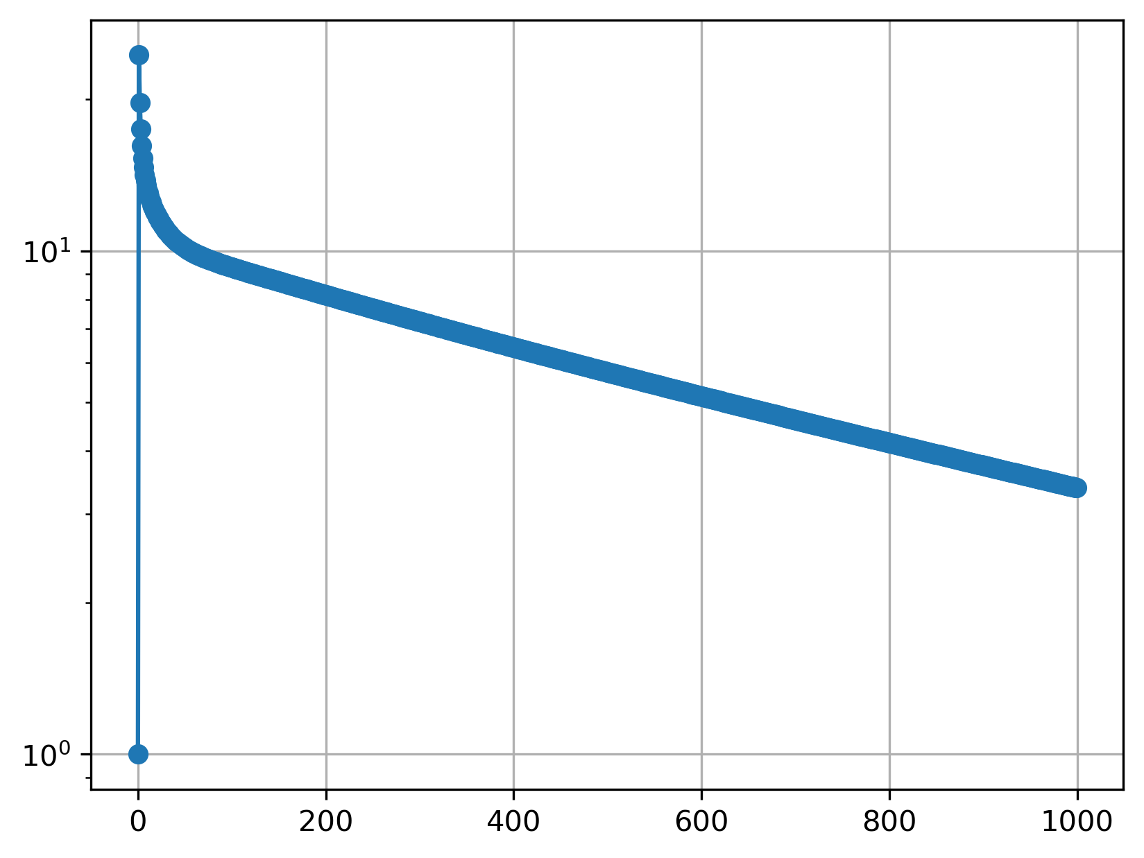
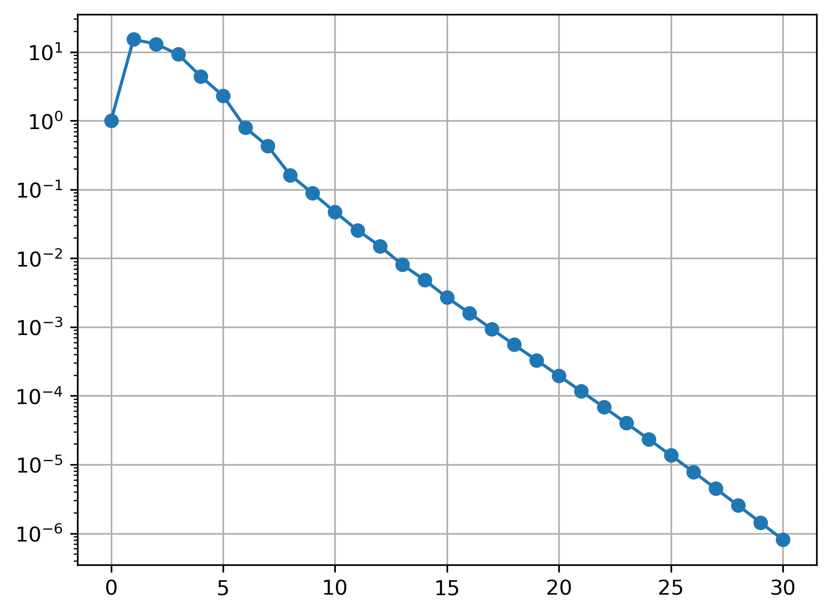
It should also be pointed out that the distribution of the coefficient determines the multi-scale property of the discrete system. The more random the distribution, the stronger the multi-scale property, making the system more challenging to solve. Figure 16 shows the behavior of FNS applied to discrete systems with different coefficients and , . The first four columns indicate that as the number of checkerboard blocks increases, the interface becomes more complex, resulting in reduced connectivity within or . Consequently, the efficiency of FNS decreases. However, as shown in the last column, if and are connected, even if the interface is highly discontinuous, the efficiency of FNS remains comparable to that of the block configuration.

5 Conclusion and discussion
In this paper, we first establish a convergence analysis framework from a spectral viewpoint for general DL-HIM. Under reasonable assumptions on smoothing operator and neural operator , the convergence rate of DL-HIM is shown to be independent of PDE parameters and grid size. Guided by this framework, we design an FFT-based neural operator to overcome spectral bias and meet the corresponding assumptions, resulted DL-HIM known as FNS. The convergence speed of FNS is guaranteed by the universal approximation and discretization invariance of the meta subnets, which requires sufficient training and is easier said than done. We verify the theoretical results and test the computational efficiency of FNS through numerical experiments on a variety of PDE discrete systems. For single-scale problems, can easily learn error components with frequencies complementary to . For multi-scale problems, needs additional help to learn a fast FNS.
FNS provides a versatile framework for solving general linear systems. However, achieving theoretical results for complex problems requires leveraging the problem characteristics and developing more suitable meta network architectures along with more efficient training algorithms. In the near future, we aim to enhance our approach to better solve multi-scale and indefinite problems. Additionally, we plan to extend the application of DL-HIM to unstructured grids and 3D problems. Furthermore, we intend to build a comprehensive software library on DL-HIM to integrate all related methods within the same framework, facilitating easier implementation and comparison. Through continuous efforts, we hope to make DL-HIM a widely used preconditioning method similar to MG and DDM, and a neural pde solver as popular as PINN and neural operators.
Acknowledgments
This work is funded by the National Natural Science Foundation of China (12371373, 12171412). KJ is partly supported by the National Key R&D Program of China (2023YFA10
08802), the Science and Technology Innovation Program of Hunan Province (2024RC1052), the Innovative Research Group Project of Natural Science Foundation of Hunan Province of China (2024JJ1008). This work was carried out in part using computing resources at the High Performance Computing Platform of Xiangtan University.
References
- [1] Y. Saad, Iterative methods for sparse linear systems, SIAM, 2003.
- [2] G. H. Golub, R. S. Varga, Chebyshev semi-iterative methods, successive overrelaxation iterative methods, and second order richardson iterative methods, Numerische Mathematik 3 (1) (1961) 157–168.
- [3] M. R. Hestenes, E. Stiefel, et al., Methods of conjugate gradients for solving linear systems, Vol. 49, NBS Washington, DC, 1952.
- [4] Y. Nesterov, A method of solving a convex programming problem with convergence rate o (1/k** 2), Doklady Akademii Nauk SSSR 269 (3) (1983) 543.
- [5] H. Luo, L. Chen, From differential equation solvers to accelerated first-order methods for convex optimization, Mathematical Programming 195 (1) (2022) 735–781.
- [6] A. Beck, L. Tetruashvili, On the convergence of block coordinate descent type methods, SIAM journal on Optimization 23 (4) (2013) 2037–2060.
- [7] G. Birkhoff, R. S. Varga, D. Young, Alternating direction implicit methods, in: Advances in computers, Vol. 3, Elsevier, 1962, pp. 189–273.
- [8] H. F. Walker, P. Ni, Anderson acceleration for fixed-point iterations, SIAM Journal on Numerical Analysis 49 (4) (2011) 1715–1735.
- [9] Y. Saad, M. H. Schultz, Gmres: A generalized minimal residual algorithm for solving nonsymmetric linear systems, SIAM Journal on scientific and statistical computing 7 (3) (1986) 856–869.
- [10] E. Chow, A. Patel, Fine-grained parallel incomplete lu factorization, SIAM journal on Scientific Computing 37 (2) (2015) C169–C193.
- [11] U. Trottenberg, C. W. Oosterlee, A. Schuller, Multigrid, Elsevier, 2000.
- [12] A. Toselli, O. Widlund, Domain decomposition methods-algorithms and theory, Vol. 34, Springer Science & Business Media, 2004.
- [13] Y. Notay, Flexible conjugate gradients, SIAM Journal on Scientific Computing 22 (4) (2000) 1444–1460.
- [14] Y. Saad, A flexible inner-outer preconditioned gmres algorithm, SIAM Journal on Scientific Computing 14 (2) (1993) 461–469.
- [15] S. Cuomo, V. S. Di Cola, F. Giampaolo, G. Rozza, M. Raissi, F. Piccialli, Scientific machine learning through physics–informed neural networks: Where we are and what’s next, Journal of Scientific Computing 92 (3) (2022) 88.
- [16] N. Kovachki, Z. Li, B. Liu, K. Azizzadenesheli, K. Bhattacharya, A. Stuart, A. Anandkumar, Neural operator: Learning maps between function spaces with applications to pdes, Journal of Machine Learning Research 24 (89) (2023) 1–97.
- [17] C. Cui, K. Jiang, S. Shu, A neural multigrid solver for helmholtz equations with high wavenumber and heterogeneous media, arXiv preprint arXiv:2404.02493 (2024).
- [18] A. Kaneda, O. Akar, J. Chen, V. A. T. Kala, D. Hyde, J. Teran, A deep conjugate direction method for iteratively solving linear systems, Proceedings of the 40th International Conference on Machine Learning 202 (2023) 15720–15736.
- [19] V. Trifonov, A. Rudikov, O. Iliev, I. Oseledets, E. Muravleva, Learning from linear algebra: A graph neural network approach to preconditioner design for conjugate gradient solvers, arXiv preprint arXiv:2405.15557 (2024).
- [20] A. Katrutsa, T. Daulbaev, I. Oseledets, Black-box learning of multigrid parameters, Journal of Computational and Applied Mathematics 368 (2020) 112524.
- [21] R. Huang, R. Li, Y. Xi, Learning optimal multigrid smoothers via neural networks, SIAM Journal on Scientific Computing (0) (2022) S199–S225.
- [22] Y. Chen, B. Dong, J. Xu, Meta-mgnet: Meta multigrid networks for solving parameterized partial differential equations, Journal of Computational Physics 455 (2022) 110996.
- [23] D. Greenfeld, M. Galun, R. Basri, I. Yavneh, R. Kimmel, Learning to optimize multigrid pde solvers, in: International Conference on Machine Learning, PMLR, 2019, pp. 2415–2423.
- [24] I. Luz, M. Galun, H. Maron, R. Basri, I. Yavneh, Learning algebraic multigrid using graph neural networks, in: International Conference on Machine Learning, PMLR, 2020, pp. 6489–6499.
- [25] A. Kopaničáková, G. E. Karniadakis, Deeponet based preconditioning strategies for solving parametric linear systems of equations, arXiv preprint arXiv:2401.02016 (2024).
- [26] A. Taghibakhshi, S. MacLachlan, L. Olson, M. West, Optimization-based algebraic multigrid coarsening using reinforcement learning, Advances in Neural Information Processing Systems 34 (2021) 12129–12140.
- [27] M. Caldana, P. F. Antonietti, et al., A deep learning algorithm to accelerate algebraic multigrid methods in finite element solvers of 3d elliptic pdes, Computers & Mathematics with Applications 167 (2024) 217–231.
- [28] H. Zou, X. Xu, C.-S. Zhang, Z. Mo, Autoamg (): An auto-tuned amg method based on deep learning for strong threshold, Communications in Computational Physics 36 (1) (2024) 200–220.
- [29] A. Klawonn, M. Lanser, J. Weber, Learning adaptive coarse basis functions of feti-dp, Journal of Computational Physics 496 (2024) 112587.
- [30] A. Taghibakhshi, N. Nytko, T. Zaman, S. MacLachlan, L. Olson, M. West, Learning interface conditions in domain decomposition solvers, Advances in Neural Information Processing Systems 35 (2022) 7222–7235.
- [31] T. Knoke, S. Kinnewig, S. Beuchler, A. Demircan, U. Morgner, T. Wick, Domain decomposition with neural network interface approximations for time-harmonic maxwell’s equations with different wave numbers, arXiv preprint arXiv:2303.02590 (2023).
- [32] A. Taghibakhshi, N. Nytko, T. U. Zaman, S. MacLachlan, L. Olson, M. West, Mg-gnn: Multigrid graph neural networks for learning multilevel domain decomposition methods, Proceedings of the 40th International Conference on Machine Learning 202 (2023) 33381–33395.
- [33] N. Rahaman, A. Baratin, D. Arpit, F. Draxler, M. Lin, F. Hamprecht, Y. Bengio, A. Courville, On the spectral bias of neural networks, in: International Conference on Machine Learning, PMLR, 2019, pp. 5301–5310.
- [34] Q. Hong, Q. Tan, J. W. Siegel, J. Xu, On the activation function dependence of the spectral bias of neural networks, arXiv preprint arXiv:2208.04924 (2022).
- [35] Z.-Q. J. Xu, Y. Zhang, T. Luo, Y. Xiao, Z. Ma, Frequency principle: Fourier analysis sheds light on deep neural networks, Communications in Computational Physics 28 (5) (2020) 1746–1767.
- [36] E. Zhang, A. Kahana, E. Turkel, R. Ranade, J. Pathak, G. E. Karniadakis, A hybrid iterative numerical transferable solver (hints) for pdes based on deep operator network and relaxation methods, arXiv preprint arXiv:2208.13273 (2022).
- [37] L. Lu, P. Jin, G. Pang, Z. Zhang, G. E. Karniadakis, Learning nonlinear operators via deeponet based on the universal approximation theorem of operators, Nature machine intelligence 3 (3) (2021) 218–229.
- [38] A. Kahana, E. Zhang, S. Goswami, G. Karniadakis, R. Ranade, J. Pathak, On the geometry transferability of the hybrid iterative numerical solver for differential equations, Computational Mechanics 72 (3) (2023) 471–484.
- [39] Z. Zou, A. Kahana, E. Zhang, E. Turkel, R. Ranade, J. Pathak, G. E. Karniadakis, Large scale scattering using fast solvers based on neural operators, arXiv preprint arXiv:2405.12380 (2024).
- [40] C. Cui, K. Jiang, Y. Liu, S. Shu, Fourier neural solver for large sparse linear algebraic systems, Mathematics 10 (21) (2022).
- [41] A. Brandt, Multi-level adaptive solutions to boundary-value problems, Mathematics of computation 31 (138) (1977) 333–390.
- [42] D. Fortunato, A. Townsend, Fast poisson solvers for spectral methods, IMA Journal of Numerical Analysis 40 (3) (2020) 1994–2018.
- [43] G. Strang, Computational science and engineering, SIAM, 2007.
- [44] Y. Xie, M. Lv, C. Zhang, Mgcnn: a learnable multigrid solver for linear pdes on structured grids, arXiv preprint arXiv:2312.11093 (2023).
- [45] A. Rudikov, V. Fanaskov, E. Muravleva, Y. M. Laevsky, I. Oseledets, Neural operators meet conjugate gradients: The fcg-no method for efficient pde solving, arXiv preprint arXiv:2402.05598 (2024).
- [46] V. Fanaskov, I. V. Oseledets, Spectral neural operators, in: Doklady Mathematics, Vol. 108, Pleiades Publishing Moscow, 2023, pp. S226–S232.
- [47] J. Hu, P. Jin, A hybrid iterative method based on mionet for pdes: Theory and numerical examples, arXiv preprint arXiv:2402.07156 (2024).
- [48] P. Jin, S. Meng, L. Lu, Mionet: Learning multiple-input operators via tensor product, SIAM Journal on Scientific Computing 44 (6) (2022) A3490–A3514.
- [49] J. Chen, Graph neural preconditioners for iterative solutions of sparse linear systems, arXiv preprint arXiv:2406.00809 (2024).
- [50] J.-T. Hsieh, S. Zhao, S. Eismann, L. Mirabella, S. Ermon, Learning neural pde solvers with convergence guarantees, International Conference on Learning Representations (2019).
- [51] M. Bolten, H. Rittich, Fourier analysis of periodic stencils in multigrid methods, SIAM journal on scientific computing 40 (3) (2018) A1642–A1668.
- [52] P. Kumar, C. Rodrigo, F. J. Gaspar, C. W. Oosterlee, On local fourier analysis of multigrid methods for pdes with jumping and random coefficients, SIAM Journal on Scientific Computing 41 (3) (2019) A1385–A1413.
- [53] J. Brown, Y. He, S. MacLachlan, Local fourier analysis of balancing domain decomposition by constraints algorithms, SIAM Journal on Scientific Computing 41 (5) (2019) S346–S369.
- [54] K. Hornik, M. Stinchcombe, H. White, Multilayer feedforward networks are universal approximators, Neural networks 2 (5) (1989) 359–366.
- [55] Z. Li, N. B. Kovachki, K. Azizzadenesheli, B. liu, K. Bhattacharya, A. Stuart, A. Anandkumar, Fourier neural operator for parametric partial differential equations, International Conference on Learning Representations (2021).
- [56] C. Cui, K. Jiang, S. Shu, Solving time-dependent parametric pdes by multiclass classification-based reduced order model, CSIAM Transactions on Applied Mathematics 4 (1) (2023) 13–40.
- [57] Y. Azulay, E. Treister, Multigrid-augmented deep learning preconditioners for the helmholtz equation, SIAM Journal on Scientific Computing (2022) S127–S151.
- [58] A. Paszke, S. Gross, F. Massa, A. Lerer, J. Bradbury, G. Chanan, T. Killeen, Z. Lin, N. Gimelshein, L. Antiga, A. Desmaison, A. Köpf, E. Yang, Z. DeVito, M. Raison, A. Tejani, S. Chilamkurthy, B. Steiner, L. Fang, J. Bai, S. Chintala, Pytorch: An imperative style, high-performance deep learning library, in: Neural Information Processing Systems, 2019.
- [59] H. Elman, D. Silvester, A. Wathen, Finite elements and fast iterative solvers: with applications in incompressible fluid dynamics (2014).
- [60] P. Wesseling, Introduction to multigrid methods, Tech. rep. (1995).