GS-ID: Illumination Decomposition on Gaussian Splatting via Diffusion Prior and Parametric Light Source Optimization

Abstract

We present GS-ID, a novel framework for illumination decomposition on Gaussian Splatting, achieving photorealistic novel view synthesis and intuitive light editing. Illumination decomposition is an ill-posed problem facing three main challenges: 1) priors for geometry and material are often lacking; 2) complex illumination conditions involve multiple unknown light sources; and 3) calculating surface shading with numerous light sources is computationally expensive. To address these challenges, we first introduce intrinsic diffusion priors to estimate the attributes for physically based rendering. Then we divide the illumination into environmental and direct components for joint optimization. Last, we employ deferred rendering to reduce the computational load. Our framework uses a learnable environment map and Spherical Gaussians (SGs) to represent light sources parametrically, therefore enabling controllable and photorealistic relighting on Gaussian Splatting. Extensive experiments and applications demonstrate that GS-ID produces state-of-the-art illumination decomposition results while achieving better geometry reconstruction and rendering performance. The source code is available at https://github.com/dukang/GS-ID.

Introduction

Reconstructing physical attributes from multiple observations has long been challenging in computer vision and computer graphics. Illumination is a highly diverse and complicated factor that significantly influences observations. Illumination Decomposition (ID) aims to achieve controllable lighting editing and produce various visual effects. However, ID is an extremely ill-posed problem, as varying interactions between different lighting distributions and materials can produce identical light effects. This issue is compounded by the complexity of illumination (e.g., self-emission, direct, and indirect illumination). Without priors of geometry and materials, this task becomes exceedingly difficult. Furthermore, the need to accurately decompose materials and geometry, solve the complex rendering equation, and consider multiple light sources and ray bounce exacerbates the challenge.

Many recent works focus on appearance reconstruction. Neural Radiance Field (NeRF) (Mildenhall et al. 2021) employs an MLP to represent a static scene as a 5D implicit light field, achieving photorealistic novel view synthesis results. 3D Gaussian Splatting (3DGS) (Kerbl et al. 2023) further incorporates explicit representation with efficient rasterization, enabling real-time rendering. However, their 3D appearance reconstruction mainly concentrates on view-dependent appearance without further decomposition.

Figure 1: GS-ID achieves high-quality delighting results under unknown illumination conditions, allowing for explicit light editing with precise control over light position, direction, and color. The thumbnails show the lighting effects of the decomposed and edited direct light sources.

To acquire a controllable light field, a well-posed geometry is necessary to support the subsequent decomposition task. Recently, 2D Gaussian Splatting (2DGS) (Huang et al. 2024) has emerged as a promising method for geometry reconstruction, utilizing surfel-based representation to ensure geometric multi-view consistency. 2DGS aims to deliver a well-posed geometry, providing significant support for ID. However, it primarily focuses on geometry reconstruction and falls short in modeling physical materials and light transport on the surface. This limitation impedes its effectiveness in more complex tasks like relighting and light editing. Another line of research (Jin et al. 2023; Jiang et al. 2024; Liang et al. 2023) on 3D inverse rendering can model both material and geometry simultaneously. However, these methods almost exclusively focus on formulating environmental illumination, struggling with user-friendly and intuitive lighting editing.

In this paper, we propose a novel framework called GS-ID, designed to decompose illumination by leveraging suitable geometry and materials from multiple observations. Our approach utilizes 2DGS for the reconstruction of geometry and materials. However, we observe that 2DGS falls short in accurately representing reflective and distant regions. To address this limitation, we incorporate a normal prior (Eftekhar et al. 2021) to obtain a well-posed geometry for subsequent decomposition tasks. For illumination decomposition, we employ a learnable panoramic map to encapsulate multiple ray-bouncing results as environmental illumination. Additionally, we use a set of Spherical Gaussians (SGs) to parametrically model direct light sources, efficiently depicting direct illumination in highlight regions. Furthermore, we adopt deferred rendering. This approach decouples the number of light sources from Gaussian points, facilitating efficient light editing and compositing.

Our GS-ID framework facilitates explicit and user-friendly light editing, enabling the composition of scenes with varying lighting effects. Experimental results demonstrate that our framework surpasses contemporary methods, offering superior control over varying illumination effects. Our contributions can be summarized as follows:

• We introduce GS-ID, a novel framework for illumination decomposition that integrates parametric direct and environmental illumination to approximate complex light fields for accurate editing and composition.

• To the best of our knowledge, we are the first to introduce the diffusion model as a prior for improving geometry and material estimation under unknown illumination.

• We employ deferred rendering, enhancing rendering performance with multiple light sources while achieving superior light editing and compositing results.

Related Work

Geometry Reconstruction Regarding surface reconstruction, some methods (Park et al. 2019; Niemeyer et al. 2020; Oechsle, Peng, and Geiger 2021; Yariv et al. 2020; Wang et al. 2021; Yariv et al. 2021) use an MLP to model an implicit field representing the target surface. After training, surfaces are extracted using isosurface extraction algorithms (Lorensen and Cline 1998; Ju et al. 2002). Recently, several methods (Huang et al. 2024; Yu, Sattler, and Geiger 2024) achieve fast and high-quality geometry reconstruction of complex scenes based on 3DGS (Kerbl et al. 2023). However, these methods often treat the appearance of a functional of view directions, neglecting the modeling of physical materials and light transport on the surface. This limitation hinders their ability to handle complex tasks such as light editing.

Intrinsic Decomposition To decompose the intrinsics from observations, some monocular methods (Zhu et al. 2022b, a; Kocsis, Sitzmann, and Nießner 2024; Zeng et al. 2024) learn from labeled datasets and estimate intrinsics directly from single images. However, these methods lack multi-view consistency and struggle to tackle out-of-distribution cases. In contrast, other methods (Bi et al. 2020; Srinivasan et al. 2021; Zhang et al. 2021, 2022; Munkberg et al. 2022; Jin et al. 2023; Jiang et al. 2024; Liang et al. 2023) construct a 3D consistent intrinsic field from multiple observations. Notably, GaussianShader and GS-IR build upon 3DGS and enable fast intrinsic decomposition on glossy areas and complex scenes. While obtaining impressive results, current methods almost only consider environmental illumination, making precise editing challenging.

Figure 2: We present GS-ID, a novel framework for illumination decomposition (ID). GS-ID decomposes the light field using environmental illumination and direct light sources, the former represented through a learnable panoramic map, and the latter modeled by a set of Spherical Gaussians. GS-ID consists of three stages. In Stage 1, we employ a modified 2DGS and an Omnidata model to reconstruct precise geometry. In Stage 2 and Stage 3, we input the G-buffer pack rendered by 2DGS and use our defined light field for physical-based rendering. This approach offers a robust understanding of the scene’s light field, enabling user-friendly editing.

Preliminaries

Gaussian Splatting

3D Gaussian Splatting (3DGS) represents a 3D scene as a collection of primitives. Each primitive models a 3D Gaussian associated with a mean vector $\bm{\mu}$, covariance matrix $\bm{\Sigma}$, opacity $\alpha$, and view-dependent color $\bm{c}$ formulated by Spherical Harmonic (SH) coefficients. Given a viewing transformation as extrinsic and intrinsic matrices $\bm{W},\bm{K}$, 3DGS efficiently projects 3D Gaussian into 2D Gaussian on the 2D screen space and performs $\alpha$-blending volume rendering to obtain the shading color $\bm{C}(\bm{u})$ of pixel $\bm{u}$:

$$\bm{C}(\bm{u}) =\sum^{N}_{i=1}T_{i}g^{\text{2D}}_{i}(\bm{u})\alpha_{i}\bm{c}_{i},\quad T_{i}=\prod^{i-1}_{j=1}\left(1-g^{\text{2D}}_{i}(\bm{u})\alpha_{j}\right),$$ (1)

$$\bm{\mu}^{\prime} =\bm{K}\bm{W}[\bm{\mu},1]^{\top},\quad\bm{\Sigma}^{\prime}=\bm{JW\Sigma W^{\top}J^{\top}},$$

$$g^{\text{2D}}(\bm{u}) =\exp{\left(-\frac{1}{2}(\bm{u}-\hat{\bm{\mu}})^{\top}\hat{\bm{\Sigma}}^{-1}(\bm{u}-\hat{\bm{\mu}})\right)},$$

where $\bm{J}$ is the Jacobian matrix of the affine approximation of the perspective projection (Zwicker et al. 2001a, b, 2002), $N$ denotes the number of Gaussians used to shade. In this work, we employ a modified 2DGS to ensure consistent geometry and output the necessary G-buffer pack, which includes materials and geometric structures, such as albedo map $\hat{\bm{A}}$, metallic map $\hat{\bm{M}}$, and roughness map $\hat{\bm{R}}$.

Physical-Based Rendering

We use Physical-Based Rendering (PBR) to model the view-dependent appearance, enabling effective illumination decomposition. We follow the rendering equation (Kajiya 1986) to model the outgoing radiance of a surface point $\bm{x}$ in direction $\bm{\omega}_{o}$:

$$L_{o}(\bm{x},\bm{\omega}_{o})=\int_{\Omega}L_{i}(\bm{x},\bm{\omega}_{i})f_{r}(\bm{\omega}_{i},\bm{\omega}_{o})(\bm{\omega}_{i}\cdot\bm{n})d\bm{\omega}_{i},$$ (2)

where $\Omega$ represents the upper hemisphere centered at point $\bm{o}$ with normal $\bm{n}$, and $\bm{\omega}_{i}$ and $\bm{\omega}_{o}$ denote the incident and view directions, respectively. The term $L_{i}(\bm{x},\bm{\omega}_{i})$ signifies the incident radiance. In particular, we use the Cook-Torrance model (Cook and Torrance 1982) to formulate the Bidirectional Reflectance Distribution Function (BRDF) $f_{r}$:

$$f_{r}(\bm{\omega}_{i},\bm{\omega}_{o}) =\underbrace{(1-M)\frac{\bm{A}}{\pi}}_{\text{diffuse component}}+\underbrace{\frac{DFG}{4(\bm{n}\cdot\bm{\omega}_{i})(\bm{n}\cdot\bm{\omega}_{o})}}_{\text{specular component}},$$ (3)

where the Normal Distribution Function $D$, Fresnel Function $F$, and Geometry Function $G$ are formulated by materials. $\bm{A}$ and $M$ represent the albedo and metallicity, respectively. Please refer to the supplemental material for more details.

Methodology

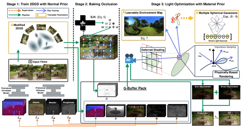
We introduce a novel three-stage framework for illumination decomposition called GS-ID. Unlike previous methods focusing solely on environmental illumination, GS-ID decomposes the light field using environmental illumination (represented by a learnable panoramic map) and parametric direct light sources (modeled by Spherical Gaussians).

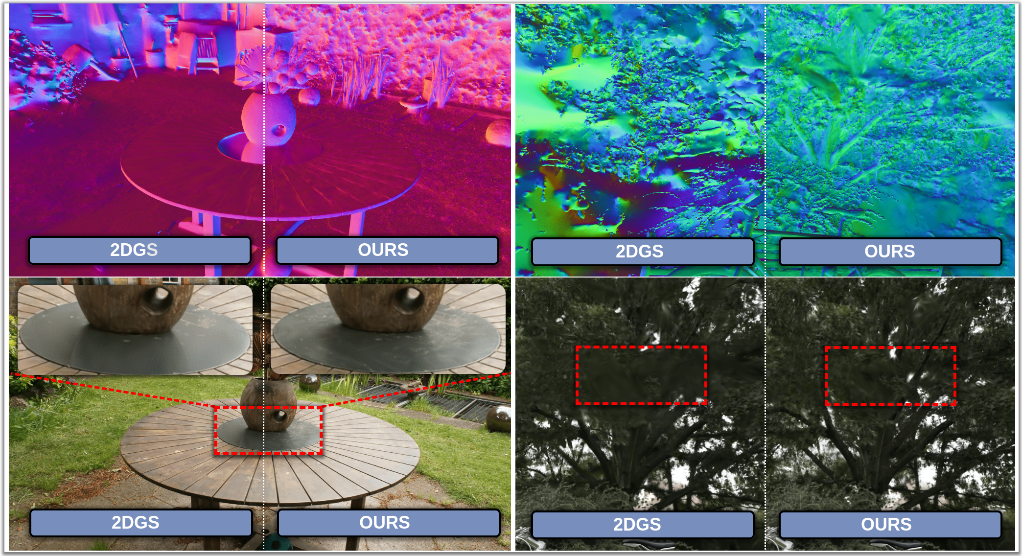
In the initial stage, we combine the normal prior from the Omnidata model (Eftekhar et al. 2021) with 2DGS (Huang et al. 2024) to produce a reasonable normal estimation. As shown in Figure 3, this approach overcomes the challenges of reconstructing textureless and glossy surfaces, which 2DGS struggles with. In the second stage, following the methodology of (Liang et al. 2023), we utilize probes to cache occlusion information, aiding in the reconstruction of ambient occlusion. In the final stage, we employ a learnable panoramic map to represent environmental illumination and a set of parametric direct light sources to model direct illumination. We then use deferred shading to render outcomes using the G-buffer pack mentioned before. Figure 2 shows the full pipeline of GS-ID.

Stage 1: Reconstruction Using Normal Prior

In this stage, we adopt 2DGS to reconstruct geometry. However, we observe that 2DGS mistakenly interprets glossy regions as holes and reduces the expressiveness of distant areas. To address these issues, we incorporate priors from a monocular geometric estimator to enhance the output geometric structures. Specifically, we use a pre-trained Omnidata model (Eftekhar et al. 2021) to provide normal supervision. Additionally, we employ Intrinsic Image Diffusion (Kocsis, Sitzmann, and Nießner 2024) to generate materials for supervising the subsequent decomposition stage. In summary, the supervision loss $\mathcal{L}_{\text{S1}}$ in Stage 1 is defined as:

$$\mathcal{L}_{\text{S1}} =\mathcal{L}_{c}+\lambda_{1}\mathcal{L}_{d}+\lambda_{2}\mathcal{L}_{n}+\lambda_{3}\mathcal{L}_{m},$$ (4)

$$\mathcal{L}_{m} =1-\hat{\bm{n}}^{T}\bm{n}_{m},$$

where $\mathcal{L}_{c}$ is an RGB reconstruction loss that combines L1 loss with the D-SSIM from 3DGS, $\mathcal{L}_{d}$ and $L_{n}$ are regularization terms from 2DGS. Simultaneously, we employ the Omnidata Model to render normal $\bm{n}_{m}$ and supervise the rendered normal $\hat{\bm{n}}$. By incorporating geometric priors, we enhance normal estimation accuracy and address geometry reconstruction challenges in textureless and distant areas, as illustrated in Figure 3. Our experimental results in Table 2 show a significant improvement in PSNR and normal accuracy compared to state-of-the-art methods. In the subsequent illumination decomposition stage, we conduct volume rendering to output the necessary G-buffer, including physical materials and geometric structures.

Figure 3: Compared with the normal produced by vanilla 2DGS, our method better handles highlights and even accurately depicts distance scenes. The second row shows that the enhanced geometry improves novel view synthesis.

Stage 2: Baking Ambient Occlusion

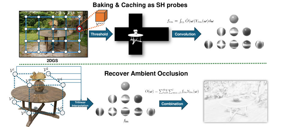
To model environmental light transport more accurately, we bake probes that precompute and store occlusion. This enhances albedo reconstruction and illumination decomposition by calculating the exposure of each point near obstructing surfaces (Figure 8). We use probes with spherical harmonics (SH) coefficients to store scene occlusion. After Stage 1, we fix the geometry (i.e., 2DGS) and regularly place occlusion probes within the bounded 3D space as $\mathcal{P}$. Each probe $\bm{p}\subset\mathcal{P}$ is designed to cache the current depth cube-map $\{\hat{D}_{i}^{\bm{p}}\}_{i=1}^{6}$. We label the depths below a certain threshold as occlusion, resulting in the occlusion cube-map $\{\hat{O}_{i}^{\bm{p}}\}_{i=1}^{6}$. Finally, we cache the occlusion in the form of SH coefficients $f_{lm}$. In the Light Optimization stage, we can recover the ambient occlusion $O(\bm{\omega})$ relative to the direction $\bm{\omega}$ as:

$$O(\bm{\omega}) =\sum_{l=0}^{deg}\sum_{m=-l}^{l}f_{lm}Y_{lm}(\bm{\omega}),$$ (5)

$$f_{lm} =\int_{\mathbb{S}^{2}}\hat{O}(\bm{\omega})Y_{lm}(\bm{\omega})d\bm{\omega},$$

where $deg$ denotes the degree of SH, $\mathbb{S}^{2}$ denotes the unit sphere, and direction $\bm{\omega}\in\mathbb{S}^{2}$ can also be written as $(\theta,\phi)$. $\{Y_{lm}(\cdot)\}$ is a set of real SH basis functions, and $\hat{O}(\bm{\omega})$ represents the occlusion query from the occlusion cube-map $\{\hat{O}_{i}^{\bm{p}}\}_{i=1}^{6}$. Practically, we perform six rendering passes and get the cube-map $\{\hat{D}_{i}^{\bm{p}}\}_{i=1}^{6}$ of occlusion probe $\bm{p}$. Then we transform it into a binary occlusion cube-map $\{\hat{O}_{i}^{\bm{p}}\}_{i=1}^{6}$ using a manually set distance threshold. In the subsequent stage, we reconstruct the ambient occlusion (AO) for each surface point from these SH probes.

Figure 4: We use SG mixture to model direct light sources. After optimization, the initially regular light sources converge to the correct distribution. Our progressive pruning scheme eliminates insignificant light sources, preserving the primary ones. In the second row, we demonstrate ID results on the Synthetic NeRF dataset, where each scene is illuminated by a direct light source.

Stage 3: Light Optimization with Material Prior

Directly solving the render equation is challenging due to the nearly infinite ray bouncing in the real world. In Stage 3, we divide light into environmental and direct illumination. Direct illumination $L^{\text{dir}}_{i}$ refers to light that directly hits the surface $\bm{x}$ with one bounce, while environmental illumination $L^{\text{env}}_{i}$ involves light reflected from media. we derive the the radiance $L_{i}$ from incidence $\bm{\omega}_{i}$ in Eq. 2 as:

$$L_{i}(\bm{x},\bm{\omega_{i}}) =L^{\text{env}}_{i}(\bm{x},\bm{\omega}_{i})\cdot\tilde{O}(\bm{\omega}_{i})+L^{\text{dir}}_{i}(\bm{x},\bm{\omega}_{i}),$$ (6)

$$L_{o}(\bm{x},\bm{\omega}_{o}) \approx L^{\text{env}}_{o}(\bm{x},\bm{\omega}_{o})\cdot O(\bm{x})+L^{\text{dir}}_{o}(\bm{x},\bm{\omega}_{o}).$$

In this context, $\tilde{O}$ represents the environmental light visibility. We approximate the integral of the occlusion term $\tilde{O}(\bm{\omega}_{i})$ using the ambient occlusion $O(\bm{x})$ obtained from Stage 2. Additionally, we employ deferred rendering to compute $L^{\text{env}}_{o}$ and $L^{\text{dir}}_{o}$ in Physically Based Rendering (PBR), utilizing the G-buffer pack. The final color, $L_{o}$, is used to calculate the loss function $\mathcal{L}_{\text{c}}$, which is a component of $\mathcal{L}_{\text{S1}}$.

Figure 5: We exemplify the estimated albedo, normal, and roughness results of GS-ID and other cutting-edge methods on real scenes. Benefitting from the intrinsic diffusion priors and our accurate light field modeling, GS-ID achieves precise geometry reconstruction and remarkable delighting results.

Environment Illumination

According to Eq. 3, environment illumination $L^{\text{env}}_{o}$ can be reformulated into its diffuse ($L^{\text{env}}_{o\text{-diff}}$) and specular ($L^{\text{env}}_{o\text{-spec}}$) components. We adopt the image-based lighting (IBL) model and split-sum approximation (Karis and Games 2013) to handle the intractable integral. $L^{\text{env}}_{o}$ can be represented as:

$$L^{\text{env}}_{o} (\bm{x},\bm{\omega}_{o})=L^{\text{env}}_{o\text{-diff}}+L^{\text{env}}_{o\text{-spec}},$$ (7)

$$L^{\text{env}}_{o\text{-diff}} \approx K^{\text{env}}_{d}I^{\text{cube}}_{d},\quad K^{\text{env}}_{d}=(1-M)\frac{\bm{A}}{\pi},$$

$$L^{\text{env}}_{o\text{-spec}} \approx\underbrace{\int_{\Omega}\frac{DFG}{4(\bm{n}\cdot\bm{l})(\bm{n}\cdot\bm{\omega}_{o})}(\bm{l}\cdot\bm{n})\,d\bm{l}}_{\text{Environment BRDF }(K^{\text{env}}_{s})}\underbrace{\int_{\Omega}DL_{i}(\bm{l})(\bm{l}\cdot\bm{n})\,d\bm{l}}_{\text{Pre-Fil. Env. Map }(I^{\text{cube}}_{s})}.$$

The term $K^{\text{env}}_{s}$ can be precomputed and stored in lookup tables, whereas $I^{\text{env}}_{d}$ and $I^{\text{env}}_{s}$ can be embedded within a learnable environment image.

Direct Illumination

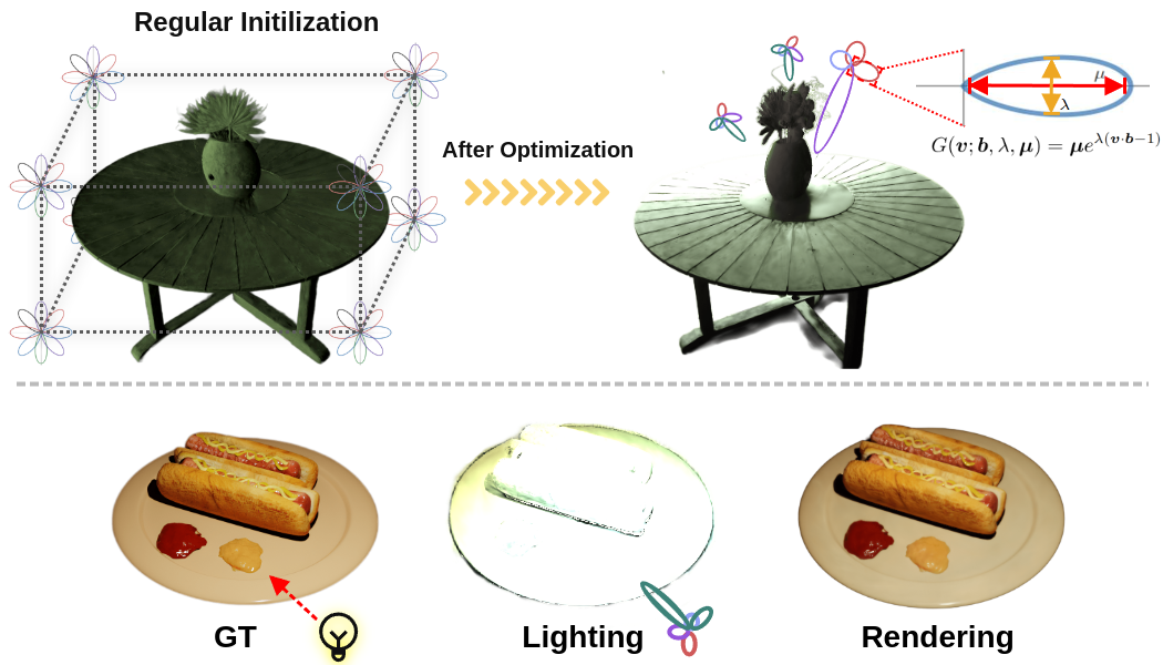
Although environmental light encompasses illumination from all directions, the absence of specific light source positions complicates lighting edits and diminishes the representation of highlights. To address this issue, we adopt the approach proposed by (Wang et al. 2009), utilizing a mixture model of scattered Spherical Gaussians (SG mixture) to simulate direct illumination with 3-channel weights representing RGB colors. Each SG mixture can be represented as a direct light source. This method enhances the expressiveness of highlights and increases the flexibility of lighting edits. Each SG mixture, consisting of $N_{\text{sg}}$ Spherical Gaussians, is formulated as:

$$\text{SGM}(\bm{\omega}_{o};\bm{b},\lambda,\bm{\mu})=\sum_{k}^{N_{\text{sg}}}\bm{\mu}_{k}e^{\lambda_{k}(\bm{\omega}_{o}\cdot\bm{b}_{k}-1)}\cdot W_{k},$$ (8)

where $W_{k}$ represents the weight of each SG in the light source. $\bm{b}_{k}\in\mathbb{S}^{2}$, $\bm{\mu}_{k}\in\mathbb{R}^{3}$, and $\lambda_{k}\in\mathbb{R}^{+}$ denote the lobe axis, amplitude, and sharpness of the $k$-th SG, respectively. As shown in Figure 4, each SG mixture efficiently simulates the direct light source.

Since we model limited and infinitesimally small light sources, the integral of direct illumination can be solved via summation according to the Importance Sampling principle (Veach 1998). The direct illumination $L^{\text{dir}}_{o}(\bm{x},\bm{\omega}_{o})$ is given by:

$$L^{\text{dir}}_{o}(\bm{x},\bm{\omega}_{o}) =\int_{\Omega}f_{r}(\bm{\omega}_{i},\bm{\omega}_{o})L_{i}^{\text{dir}}(\bm{x},\bm{\omega}_{i})(\bm{n}\cdot\bm{\omega}_{i})d\bm{\omega}_{i},$$ (9)

$$=\frac{1}{N_{\text{light}}}\sum_{j}^{N_{\text{light}}}\frac{f_{r,j}\cdot\text{SGM}(\bm{\omega}_{o,j};j)(\bm{n}\cdot\bm{\omega}_{i,j})}{p_{j}d_{j}^{2}},$$

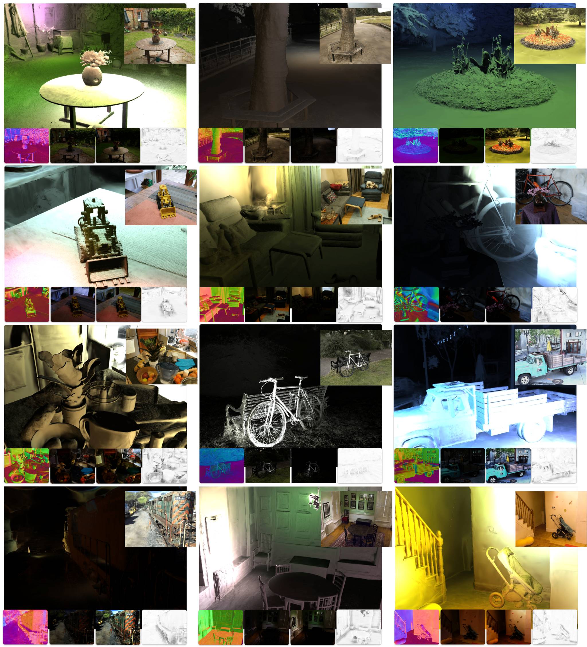
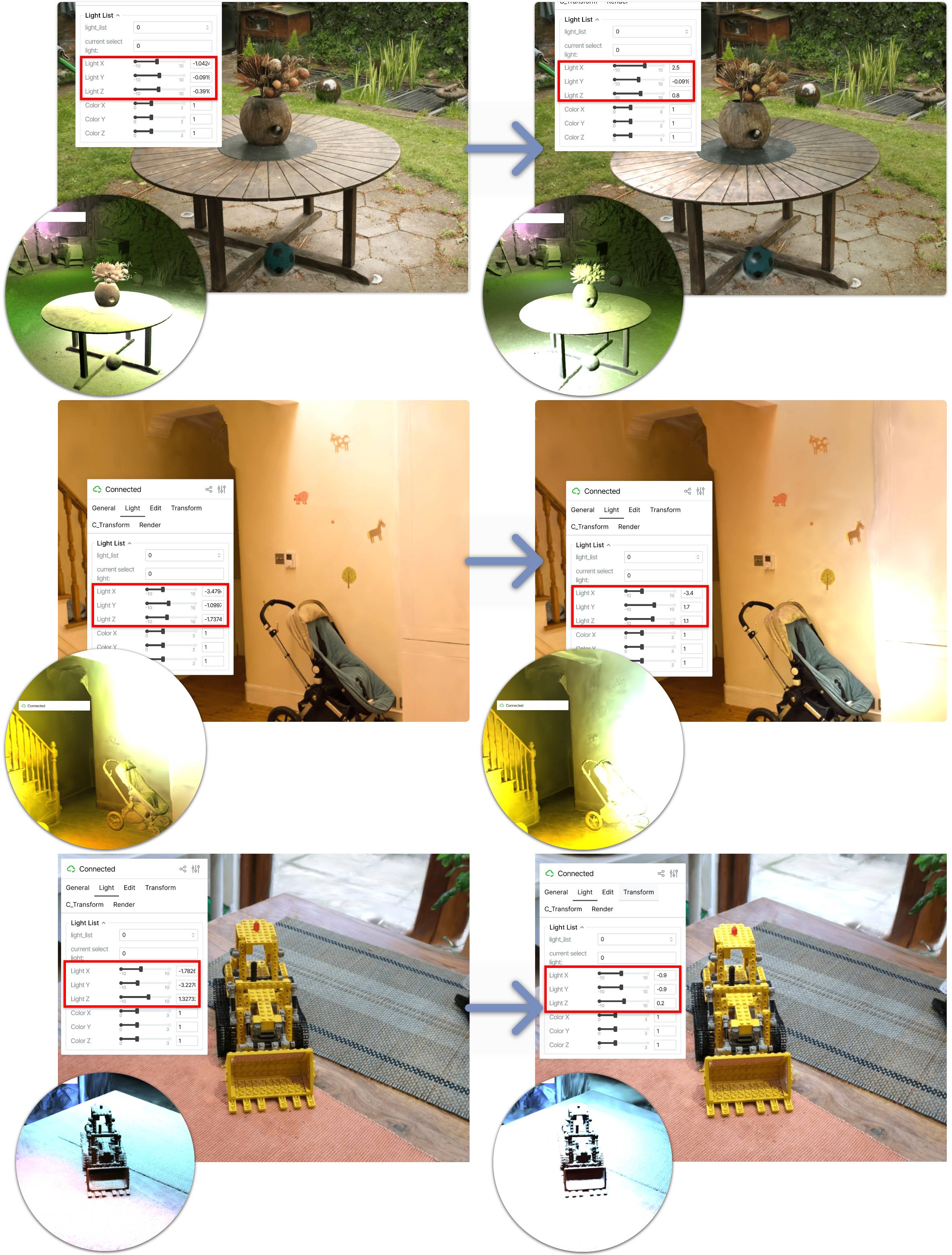
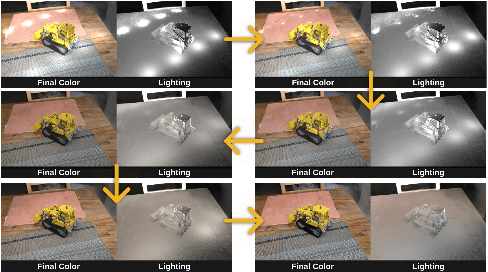
where $N_{\text{light}}$ denotes the number of direct light sources (SG mixtures), and $f_{r,j}$ represents the $j$-th light source’s coefficients that conform to the BRDF Cook-Torrance microfacet model (Walter et al. 2007) defined in Eq. 3. $p_{j}$ represents the probability density function (PDF) for sampling the direct light source, and $d_{i}$ is the distance between the surface and the $i$-th light source. Specifically, Eq. 9 can be efficiently solved using deferred ray tracing techniques (Pharr 2005). By learning the parametric direct light, as shown in Figure 1 and Figure 6, we can accurately separate direct illumination, allowing us to explicitly edit the light within the scene.

To enhance illumination decomposition, we employ a dense light source initialization strategy. Specifically, we divide the bounded 3D space into a regular grid and place an SG mixture representing direct light sources at each grid point, ensuring comprehensive scene coverage. Each SG mixture includes $N_{\text{sg}}$ SGs with varying weights. During optimization, the parameters of each SG and the positions of the light sources are trainable. Given that most real-world scenarios feature few significant light sources, we introduce a progressive pruning scheme to eliminate weak light sources, thereby improving decomposition efficiency and editing friendliness. Our experiments demonstrate that the light sources gradually converge to plausible locations, producing accurate visual effects as shown in Figure 4. For more details, please refer to the supplementary materials.

Figure 6: The results show that we accurately separate direct illumination and recover lighting effects. Notably, we show the results in linear space to emphasize the lighting effects, thus the illuminated areas are prominent.

Losses

In Stage 3, our objective is to develop a lighting representation that is both controllable and richly expressive, capturing the nuanced interplay of light within the scene. To achieve this, we adopt the regularization term proposed by (Kocsis, Sitzmann, and Nießner 2024):

$$\mathcal{L}_{\text{pos}} =\sum_{i}^{N_{\text{light}}}1/d_{i},\quad\mathcal{L}_{\text{val}}=\sum_{i}^{N_{\text{light}}}\sum_{j}^{N_{\text{sg}}}\|W_{i,j}\|_{2},$$ (10)

$$\mathcal{L}_{\text{light}}=\lambda_{\text{pos}}\mathcal{L}_{\text{pos}}+\lambda_{\text{val}}\mathcal{L}_{\text{val}},$$

where $d_{i}$ denotes the distance between the light source and the nearest surface point, and $W_{i,j}$ denotes the weight of each SG. For decomposition, we introduce intrinsic diffusion priors to alleviate the ill-posedness:

$$\mathcal{L}_{\text{reg}} =\lambda_{R}L_{2}{(R,\hat{R})}+\lambda_{M}L_{2}{(M,\hat{M})}+\lambda_{\bm{A}}L_{2}{(\bm{A},\hat{\bm{A}})},$$ (11)

where $\hat{R},\hat{M},\hat{\bm{A}}$ denote the predicted roughness, metallicity and albedo, respectively. $R,M,\bm{A}$ are the pseudo material supervision produced by Intrinsic Image Diffusion. Primarily, we follow Eq. 4 to finely optimize the geometry and appearance jointly in Stage 3. Combining with Eqs. 4, 10, and 11, the summary loss $\mathcal{L}_{\text{S3}}$ in Stage 3 is:

$$\mathcal{L}_{\text{S3}}= \mathcal{L}_{\text{S1}}+\mathcal{L}_{\text{light}}+\mathcal{L}_{\text{reg}}.$$ (12)

Method	Normal	Novel View Synthesis			Albedo
	MAE$\downarrow$	LPIPS$\downarrow$	PSNR$\uparrow$	SSIM$\uparrow$	LPIPS$\downarrow$	PSNR$\uparrow$	SSIM$\uparrow$
NeRFactor	6.314	0.120	24.68	0.922	0.109	25.13	0.940
InvRender	5.074	0.089	27.37	0.934	0.100	27.34	0.933
NVDiffrec	6.078	0.052	30.70	0.962	0.115	29.17	0.908
TensoIR	4.100	0.040	35.09	0.976	0.085	29.28	0.950
GS-IR	4.948	0.039	35.33	0.974	0.084	30.29	0.941
Ours	4.120	0.027	36.72	0.977	0.094	30.62	0.940

Table 1: Quantitative comparison on the TensoIR Synthetic dataset shows our method achieves the best results in novel view synthesis and albedo quality, and second-best for normal reconstruction.

	Outdoor Scene			Indoor Scene
	PSNR$\uparrow$	SSIM$\uparrow$	LIPPS$\downarrow$	PSNR$\uparrow$	SSIM$\uparrow$	LIPPS$\downarrow$
NeRF	21.46	0.458	0.515	26.84	0.790	0.370
Deep Blending	21.54	0.524	0.364	26.40	0.844	0.261
Instant NGP	22.90	0.566	0.371	29.15	0.880	0.216
Mip-NeRF 360	24.47	0.691	0.283	31.72	0.917	0.180
3DGS†	24.64	0.731	0.234	30.41	0.920	0.189
2DGS†	24.34	0.717	0.246	30.40	0.916	0.195
Ours-S1†	24.48	0.718	0.252	30.84	0.921	0.188
GaussianShader†	22.80	0.665	0.297	26.19	0.876	0.243
GSIR†	23.45	0.671	0.284	27.46	0.863	0.237
Ours-S3†	23.58	0.673	0.299	28.84	0.894	0.220

Table 2: Quantitative results on Mip-NeRF 360 dataset. Methods with ^† achieve real-time rendering, and the methods in the second block enable lighting editing.

Method	TensoIR Synthetic				Mip-NeRF 360
	Normal	Albedo			Novel View Synthesis
	MAE$\downarrow$	PSNR$\uparrow$	SSIM$\uparrow$	LPIPS$\downarrow$	PSNR$\uparrow$	SSIM$\uparrow$	LPIPS$\downarrow$
w/o normal supervision	4.157	30.540	0.923	0.095	25.262	0.752	0.277
w/o material supervision	4.267	28.889	0.918	0.099	25.228	0.750	0.268
w/o direct illu.	4.186	30.191	0.925	0.096	24.870	0.749	0.287
w/o env illu.	4.161	30.320	0.923	0.096	25.127	0.762	0.273
forward shading	4.310	27.988	0.916	0.101	24.880	0.748	0.269
Ours	4.120	30.625	0.935	0.094	25.914	0.771	0.263

Table 3: Analyses on the impact of different schemes during the training process. In detail, normal and material denote priors from the pretrained Omnidata model and the intrinsic diffusion model, env illu. and direct illu. are the illumination represented by the panoramic map and SGs.

Experiments

Dataset and Metrics

We conduct experiments on real-world datasets, such as Mip-NeRF 360 (Barron et al. 2022), to evaluate our illumination decomposition approach. Our evaluation metrics include PSNR, SSIM, and LPIPS (Zhang et al. 2018). Additionally, we utilize the TensoIR (Jin et al. 2023) synthetic dataset for comparative analysis of illumination decomposition. This dataset features scenes rendered with Blender under various lighting conditions, along with ground truth normals and albedo.

Figure 7: The first column demonstrates the precise editing of direct light through the control panel. In the second column, it reveals that two GS scenes can be composited during runtime and share illumination sources.

Comparisons

Our work aims to improve normal accuracy in Stage 1 and emphasize illumination decomposition in Stage 3. To evaluate this, we conduct comparisons using public datasets. First, we use the Mip-NeRF 360 datasets to compare novel view synthesis results and normal estimation in Stage 1, contrasting our approach with 2DGS and other contemporary methods. Then we use Mip-NeRF 360 and TensorIR Synthetic datasets to compare novel view synthesis results and ID comparison outcomes in Stage 3.

Comparison in geometry reconstruction

In Stage 1, as shown in Figure 3, incorporating the pretrained Omnidata model (Eftekhar et al. 2021) as geometric priors improves normal estimation in glossy and distant areas. We evaluate novel view synthesis results and Table 2 presents quantitative comparisons on the Mip-NeRF 360 dataset. Our results demonstrate improvements compared to the vanilla 2DGS method. Importantly, our approach excels in indoor scenes due to the use of diffusion models optimized for indoor environments.

Comparison in light optimization

With the improved geometry structure from Stage 1, we achieve remarkable illumination decomposition results. In the TensoIR Synthetic dataset, our approach excels in novel view synthesis and albedo estimation, achieving the second-best normal estimation. Table 1 demonstrates our precise illumination decomposition capabilities, using the same metrics for evaluating albedo quality as for novel view synthesis.

We utilize the Mip-NeRF 360 dataset to evaluate real-world scenes with complex lighting. As depicted in Figure 6, we accurately identify regions of direct and environmental illumination. Table 2 shows that, compared to recent relighting works such as (Liang et al. 2023; Jiang et al. 2024), our method in Stage 3 achieves superior quality. Furthermore, we successfully decompose materials, including albedo, metallicity, and roughness. As illustrated in Figure 5, our real-world decomposition enhances albedo, roughness, and normal components compared to other concurrent works. Additionally, we can explicitly determine the location and intensity of the light source, enabling editable light editing and scene composition. For a more comprehensive understanding, more applications are showcased in the supplement.

Ablation Studies

We introduce 2DGS for illumination decomposition (ID) and propose supervision training using a diffusion model as priors. Our method is evaluated on TensorIR Synthetic and Mip-NeRF 360 datasets, demonstrating its effectiveness in ID tasks. The following sections present a detailed ablation study on geometry and material priors, direct illumination, environment illumination, and deferred rendering.

Analysis on Normal and Material Regularization

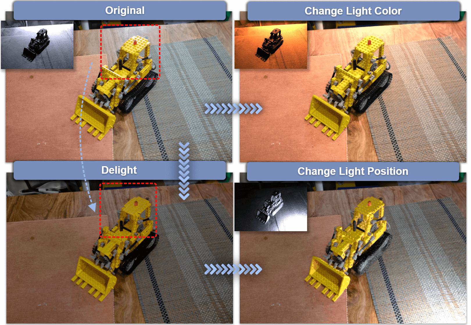
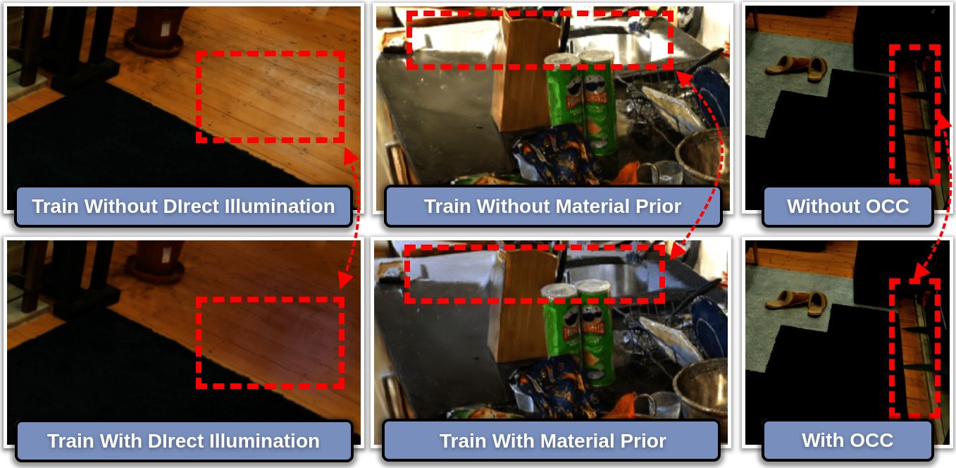
Accurate estimation of normals and materials is crucial for illumination decomposition (ID). To achieve this, we introduce intrinsic diffusion priors to guide the 2DGS normal and material estimation. In this section, we examine the effects of various acquisition schemes on normal, color quality, and albedo quality. Table 3 shows that the introduced prior improves normal estimation and ID results. Moreover, the albedo outcome for the TensoIR dataset is significantly lower when compared to using a material prior. Notably, the absence of a material prior results in decreased quality of novel view synthesis. The delighting results for the Mip-NeRF 360 dataset are also inferior, as shown in Figure 8.

Analysis on Direct and Environmental Illumination

In Stage 3, we assume that the illumination consists of direct and environmental components with occlusion. To test the impact of different illumination and occlusion on ID, we explore various combination schemes. As demonstrated in Table 3 and Figure 8, removing direct illumination or occlusion both leads to poorer albedo quality, resulting in deteriorated ID outcomes. Direct illumination can better identify Bloom regions and effectively remove the highlights from the albedo. Occlusion can recognize environmental shadows and effectively reduce shadow effects.

Analysis on Deferred Rendering

During the decomposition process, we employ the deferred shading technique instead of the forward shading approach typically used in earlier methods. In this context, we investigate its impact on light editing. As shown in Table 3, deferred rendering yields superior ID results and enhanced quality in all metrics.

Figure 8: The first two columns compare albedo results with and without direct illumination, as well as with and without material priors during training, thereby verifying the effectiveness of our scheme in delighting. Finally, the last column demonstrates that ambient occlusion effectively reduces shadows in the albedo.

Applications

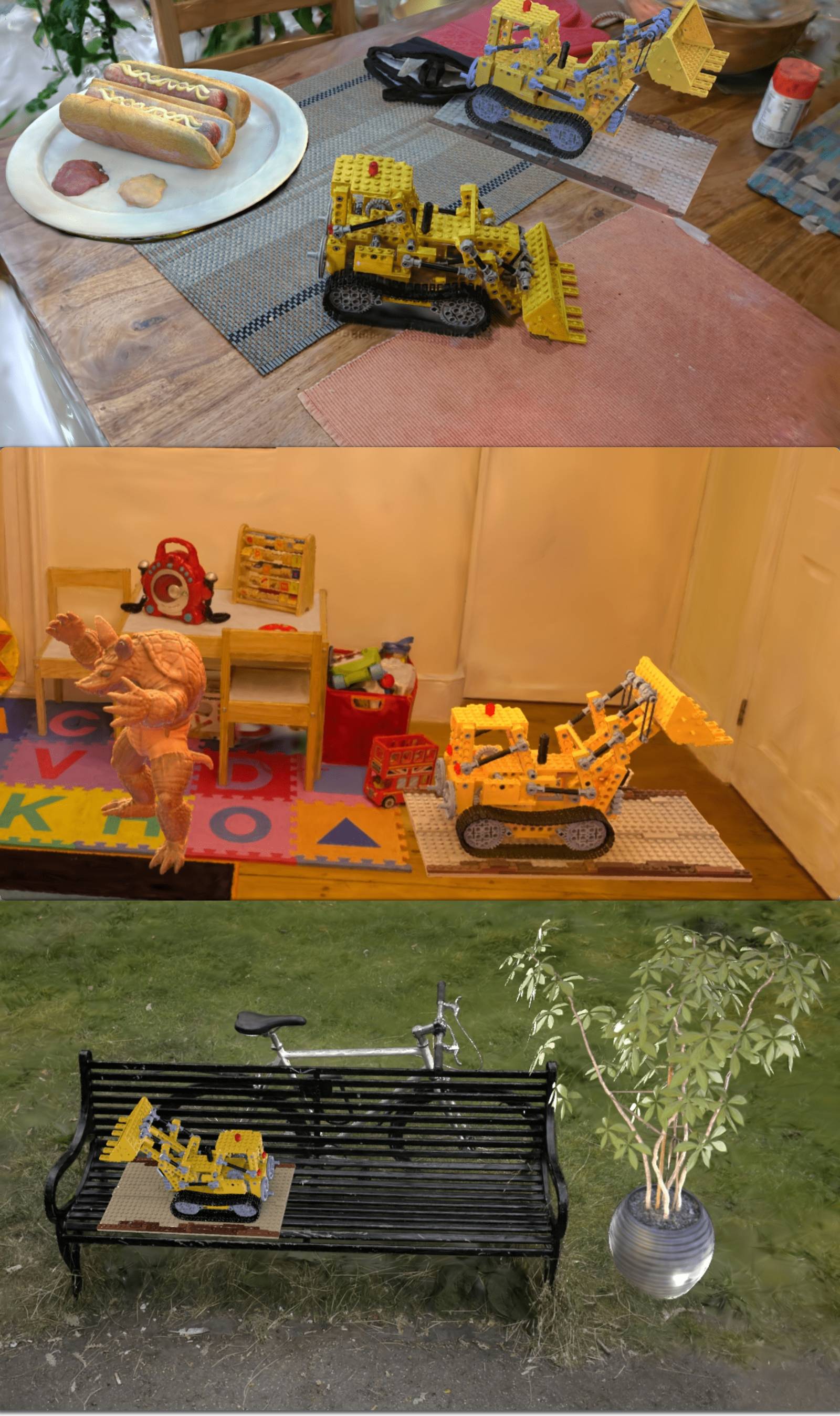
We conduct light editing applications using the recovered geometry, material, and illumination from our GS-ID. As shown in Figure 7, the results demonstrate that GS-ID effectively handles precise light editing, generating photorealistic renderings. Furthermore, our parametric light sources allows for illumination extraction from one decomposed scene and integration into another scene without additional training. More results can be found in the supplementary materials.

Conclusion

We introduce GS-ID, a novel three-stage framework for illumination decomposition that enables photorealistic novel view synthesis, intuitive light editing, and scene composition. GS-ID integrates 2D Gaussian Splatting with intrinsic diffusion priors to regularize normal and material estimation. We decompose the light field into environmental and direct illumination, employing parametric modeling and optimization schemes for enhanced illumination decomposition. Additionally, GS-ID utilizes deferred rendering in screen space to achieve high rendering performance. Our work has a few limitations. For example, GS-ID relies on the priors from intrinsic diffusion methods, which fails to generalize to out-of-distribution cases, resulting in degeneration decomposition. Our future work includes improving the applicability of GS-ID. We plan to explore various applications, such as simulating a wide range of parametric light sources (e.g., area light) to increase the diversity of lighting effects. Furthermore, we will consider the visibility between direct lights and surface points to integrate shadow effects into novel view synthesis, ensuring more realistic and harmonic results, especially for the scene composition.

Supplementary Material

In this supplementary material, we first present the implementation details of our method. This is followed by additional results from various datasets. We also provide further qualitative results on material prediction, including factors such as albedo, normals properties, and lighting conditions for both synthetic and realistic datasets. Finally, we offer more application results. Additional videos demonstrating our work can be found in the supplementary material HTML file (main.html).

Implementation Details

We implement Gaussian ID using the PyTorch framework with CUDA extensions and modify 2DGS to output G-buffer properties, including roughness, metallic, normal, depth, and ambient occlusion.

Representation

In the vanilla 2DGS, each 2D Gaussian utilizes learnable parameters $\mathcal{T}=\{\bm{p},\bm{s},\bm{q},\bm{n},\bm{d}\}$ and $\mathcal{C}=\{\alpha,\bm{f}_{c}\}$ to describe its geometric properties and volumetric appearance, respectively. Here, $\bm{p}$ denotes the position vector, $\bm{s}$ denotes the scaling vector, $\bm{q}$ denotes the unit quaternion for rotation, $\bm{n}$ denotes the normal, $\bm{d}$ denotes the depth, $\alpha$ denotes the opacity, and $\bm{f}_{c}$ denotes the spherical harmonics (SH) coefficients for view-dependent color. In GS-ID, we extend $\mathcal{C}$ to $\{\alpha,\bm{f}_{c},\bm{A},R,M\}$ to describe the material properties of the 2D Gaussian.

Training Details

We employ Physically-Based Rendering (PBR) to model the view-dependent appearance, facilitating effective illumination decomposition. Specifically, we utilize the Cook-Torrance model to formulate the Bidirectional Reflectance Distribution Function (BRDF) $f_{r}$:

$$f_{r}(\bm{\omega}_{i},\bm{\omega}_{o}) =\underbrace{(1-M)\frac{\bm{A}}{\pi}}_{\text{diffuse component}}+\underbrace{\frac{DFG}{4(\bm{n}\cdot\bm{\omega}_{i})(\bm{n}\cdot\bm{\omega}_{o})}}_{\text{specular component}},$$ (13)

$$\bm{h} =\text{normalize}(\bm{\omega}_{o}+\bm{\omega}_{i}),$$

$$F_{0} =(1-M)*0.04+M*\bm{A},$$

$$D(\bm{n},\bm{h}) =\frac{R^{4}}{\pi\left(\bm{n}\cdot\bm{h}\ (R^{4}-1)+1\right)^{2}},$$

$$F(\bm{\omega}_{i},\bm{n}) =F_{0}+(1-F_{0})\left(1-\bm{n}\cdot{\bm{\omega}_{i}}\right)^{5},$$

$$G(\bm{\omega}_{o},\bm{\omega}_{i},\bm{h}) =G_{1}(\bm{\omega}_{o},\bm{h})\ G_{1}(\bm{\omega}_{i},\bm{h}),$$

$$G_{1}(\bm{n},\bm{h}) =\frac{1}{1+\bm{n}\cdot\bm{h}\sqrt{R^{4}+\bm{n}\cdot\bm{h}-R^{4}*\bm{n}\cdot\bm{h}}},$$

where $\bm{A}$, $R$, and $M$ denote the albedo, roughness, and metallicity, respectively. The Normal Distribution Function (NDF) $D$, Fresnel function $F$, and Geometry function $G$ are derived from physical materials. For training, we utilize the Adam optimizer, and the training process is divided into three stages.

Stage 1 As outlined in the Methodology section, we aim to minimize the color reconstruction loss ($L_{c}$) and the normal loss ($L_{n}$). The normal loss is composed of $\lambda_{1}L_{d}+\lambda_{2}L_{n}+\lambda_{3}L_{m}$, where $\lambda_{3}L_{m}$ represents the loss supervised by the Omnidata Model. This supervision is crucial for maintaining geometric consistency, particularly in the glossy and distant regions of the reconstructed 2DGS geometry. We use $\lambda_{1}=100$, $\lambda_{2}=0.25$, and $\lambda_{3}=0.25$. To optimize the parameters $\mathcal{T}$ and $\mathcal{C}$ from 2DGS, we perform this minimization for 30k iterations.

Stage 2 In Stage 2, we introduce spherical harmonics (SH) architectures and cache occlusion into occlusion volumes $\mathcal{V}^{\text{occl}}$, as illustrated in Fig. 10. For each volume $\bm{v}^{\text{occl}}_{i}\subset\mathcal{V}^{\text{occl}}$, we position six cameras with a field of view (FoV) of $90^{\circ}$, ensuring they do not overlap. We then perform six render passes to obtain the depth cubemap $\{\hat{\bm{D}}^{i}_{p}\}_{p=1}^{6}$. By comparing the values of the depth map with a threshold, we convert $\{\hat{\bm{D}}^{i}_{p}\}_{p=1}^{6}$ into the occlusion cubemap $\{\hat{\bm{O}}^{i}_{p}\}_{p=1}^{6}$ and store the principal components of occlusion in spherical harmonics (SH) coefficients $\bm{f}_{lm}$ within the volume.

Stage 3 We employ a mixture model of scattered Spherical Gaussians (SG mixture) to represent the direct illumination as $L^{\text{dir}}_{o}(\bm{x},\bm{\omega}_{o})$:

$$L^{\text{dir}}_{o}(\bm{x},\bm{\omega}_{o}) =\frac{1}{N_{\text{light}}}\sum_{i}^{N_{\text{light}}}\frac{K^{\text{dir}}_{i}(\bm{n}\cdot\bm{\omega}_{i})}{{d}_{i}^{2}}\sum_{j}^{N_{\text{sg}}}W_{i,j}SG(j),$$ (14)

where $d_{i}$ denotes the distance from the $i$-th light source cluster to the surface point $\bm{x}$. The probability density function (PDF) is 1.0 for a point light source. $K$ and $SG$ denote the BRDF function and the Spherical Gaussian Function, respectively, as defined in the Methodology section. Utilizing pretrained models $\mathcal{T}$ and $\mathcal{C}$, along with material properties generated by a pretrained diffusion model, we optimize $M$ and $L$ over 30,000 iterations. The optimization is guided by the following loss function:

$$\mathcal{L}_{\text{reg}} =\lambda_{R}L2(R,\hat{R})+\lambda_{M}L2(M,\hat{M})+\lambda_{\bm{A}}L2(\bm{A},\hat{\bm{A}}),$$ (15)

where the weights for the loss function are set as: $\lambda_{R}=0.1$, $\lambda_{M}=0.1$, and $\lambda_{\bm{A}}=0.5$. The entire illumination optimization process can be visualized as shown in Fig. 9.

Figure 9: We optimize for $N_{\text{light}}$ light sources with a Spherical Gaussian (SG) mixture, in conjunction with environmental lighting. Our representation is sufficiently expressive to capture detailed emissions while remaining controllable for light editing purposes.

Results on MipNeRF 360, DB and T&T Dataset

Tabs. 4, 5, and 6 present the results for novel view synthesis using the Mip-NeRF 360 Dataset. Tabs. 7, 8, and 9 display the results for Deepblend and the T&T Dataset. Additionally, Fig. 11 illustrates the ID results for these scenes.

Results on TensoIR Synthetic Dataset

Tab. 10 presents the outcomes for normal estimation, novel view synthesis, albedo reconstruction, and relighting across all four scenes.

Method	bicycle	flowers	garden	stump	treehill	room	counter	kitchen	bonsai
NeRF++	22.64	20.31	24.32	24.34	22.20	28.87	26.38	27.80	29.15
Plenoxels	21.91	20.10	23.49	20.66	22.25	27.59	23.62	23.42	24.67
INGP-Base	22.19	20.35	24.60	23.63	22.36	29.27	26.44	28.55	30.34
INGP-Big	22.17	20.65	25.07	23.47	22.37	29.69	26.69	29.48	30.69
Mip-NeRF 360	24.40	21.64	26.94	26.36	22.81	29.69	26.69	29.48	30.69
3DGS	25.25	21.52	27.41	26.55	22.49	30.63	28.70	30.32	31.98
2DGS	24.87	21.15	26.95	26.47	22.27	31.06	28.55	30.50	31.52
Gaussian ID-S1	24.98	21.41	27.03	26.54	22.44	31.40	28.85	31.10	31.99
Gaussian Shader	23.12	20.34	26.44	23.92	20.17	24.27	26.35	27.72	28.09
GSIR	23.80	20.57	25.72	25.37	21.79	28.79	26.22	27.99	28.18
Gaussian ID-S3	24.26	20.90	26.36	24.35	22.01	29.88	27.26	29.02	29.19

Table 4: PSNR scores for Mip-NeRF360 scenes.

Method	bicycle	flowers	garden	stump	treehill	room	counter	kitchen	bonsai
NeRF++	0.526	0.453	0.635	0.594	0.530	0.530	0.802	0.816	0.876
Plenoxels	0.496	0.431	0.606	0.523	0.509	0.842	0.759	0.648	0.814
INGP-Base	0.491	0.450	0.649	0.574	0.518	0.855	0.798	0.818	0.890
INGP-Big	0.512	0.486	0.701	0.594	0.542	0.871	0.817	0.858	0.906
Mip-NeRF 360	0.693	0.583	0.816	0.746	0.632	0.913	0.895	0.920	0.939
3DGS	0.771	0.605	0.868	0.775	0.638	0.914	0.905	0.922	0.938
2DGS	0.752	0.588	0.852	0.765	0.627	0.912	0.900	0.919	0.933
Gaussian ID-S1	0.750	0.594	0.851	0.763	0.623	0.916	0.904	0.924	0.939
Gaussian Shader	0.700	0.542	0.842	0.667	0.572	0.847	0.874	0.887	0.893
GSIR	0.706	0.543	0.804	0.716	0.586	0.867	0.839	0.867	0.883
Gaussian ID-S3	0.721	0.561	0.826	0.665	0.586	0.896	0.874	0.897	0.910

Table 5: SSIM scores for Mip-NeRF360 scenes.

Method	bicycle	flowers	garden	stump	treehill	room	counter	kitchen	bonsai
NeRF++	0.455	0.466	0.331	0.416	0.466	0.335	0.351	0.260	0.291
Plenoxels	0.506	0.521	0.386	0.503	0.540	0.419	0.441	0.447	0.398
INGP-Base	0.487	0.481	0.312	0.450	0.489	0.301	0.342	0.254	0.227
INGP-Big	0.446	0.441	0.257	0.421	0.450	0.261	0.306	0.195	0.205
Mip-NeRF 360	0.289	0.345	0.164	0.254	0.338	0.211	0.203	0.126	0.177
3DGS	0.205	0.336	0.103	0.210	0.317	0.220	0.204	0.129	0.205
2DGS	0.218	0.346	0.115	0.222	0.329	0.223	0.208	0.133	0.214
Gaussian ID-S1	0.228	0.346	0.121	0.226	0.341	0.219	0.203	0.130	0.206
Gaussian Shader	0.274	0.377	0.130	0.297	0.406	0.304	0.242	0.167	0.257
GSIR	0.259	0.371	0.158	0.258	0.372	0.279	0.260	0.188	0.264
Gaussian ID-S3	0.256	0.368	0.144	0.329	0.400	0.247	0.232	0.157	0.244

Table 6: LPIPS scores for Mip-NeRF360 scenes.

Method	Trucks	Train	Avg.	Drjohnson	Playroom	Avg.
3DGS	25.18	21.09	23.13	28.76	30.04	29.40
2DGS	24.78	21.67	23.22	29.02	30.23	29.62
Gaussian ID-S1	25.19	21.73	23.46	29.16	30.24	29.70
Gaussian Shader	20.13	23.56	21.84	22.18	19.88	21.03
GSIR	24.09	20.42	22.25	26.47	28.13	27.30
Gaussian ID-S3	24.51	23.60	22.71	28.05	28.55	28.30

Table 7: PSNR scores for DB and T&T Dataset.

Method	Trucks	Train	Avg.	Drjohnson	Playroom	Avg.
3DGS	0.879	0.802	0.840	0.899	0.906	0.902
2DGS	0.867	0.803	0.835	0.901	0.907	0.904
Gaussian ID-S1	0.875	0.807	0.841	0.902	0.902	0.902
Gaussian Shader	0.763	0.843	0.803	0.786	0.845	0.815
GSIR	0.833	0.742	0.787	0.863	0.869	0.866
Gaussian ID-S3	0.858	0.778	0.818	0.886	0.885	0.885

Table 8: SSIM scores for DB and T&T Dataset.

Method	Trucks	Train	Avg.	Drjohnson	Playroom	Avg.
3DGS	0.148	0.218	0.183	0.244	0.241	0.242
2DGS	0.183	0.227	0.205	0.248	0.250	0.249
Gaussian ID-S1	0.170	0.222	0.196	0.252	0.257	0.254
Gaussian Shader	0.271	0.191	0.231	0.336	0.359	0.344
GSIR	0.195	0.273	0.234	0.314	0.305	0.309
Gaussian ID-S3	0.182	0.250	0.216	0.268	0.271	0.269

Table 9: LPIPS scores for DB and T&T Dataset.

Figure 10: Ambient Occlusion recovery from occlusion probes in the baking stage.

		Normal (MAE)	Novel View Synthesis			Albedo
			PSNR	SSIM	LPIPS	PSNR	SSIM	LPIPS
Lego	NeRFactor	9.767	26.076	0.881	0.151	25.444	0.937	0.112
	InvRender	9.980	24.391	0.883	0.151	21.435	0.882	0.160
	TensoIR	5.980	34.700	0.968	0.037	25.240	0.900	0.145
	GS-IR	8.078	34.379	0.968	0.036	24.958	0.889	0.143
	Gaussian ID-S3	6.680	35.415	0.972	0.027	22.581	0.908	0.150
Hotdog	NeRFactor	5.579	24.498	0.940	0.141	24.654	0.950	0.142
	InvRender	3.708	31.832	0.952	0.089	27.028	0.950	0.094
	TensoIR	4.050	36.820	0.976	0.045	30.370	0.947	0.093
	GS-IR	4.771	34.116	0.972	0.049	26.745	0.941	0.088
	Gaussian ID-S3	4.701	36.617	0.978	0.032	23.296	0.913	0.119
Armadillo	NeRFactor	3.467	26.479	0.947	0.095	28.001	0.946	0.096
	InvRender	1.723	31.116	0.968	0.057	35.573	0.959	0.076
	TensoIR	1.950	39.050	0.986	0.039	34.360	0.989	0.059
	GS-IR	2.176	39.287	0.980	0.039	38.572	0.986	0.051
	Gaussian ID-S3	2.370	40.803	0.982	0.032	43.752	0.980	0.061
Ficus	NeRFactor	6.442	21.664	0.919	0.095	22.402	0.928	0.085
	InvRender	4.884	22.131	0.934	0.057	25.335	0.942	0.072
	TensoIR	4.420	29.780	0.973	0.041	27.130	0.964	0.044
	GS-IR	4.762	33.551	0.976	0.031	30.867	0.948	0.053
	Gaussian ID-S3	2.746	34.037	0.976	0.017	32.876	0.959	0.045

Table 10: Per-scene results on TensoIR Synthetic dataset. For albedo reconstruction results, we follow NeRFactor and scale each RGB channel by a global scalar.

Applications

Light Editing

Utilizing a Spherical Gaussian (SG) mixture for lighting offers a flexible and controllable method for representing scene illumination. Upon completion of the training process, the emission weights, positions, and SG parameters of the light sources can be independently adjusted. This emissive representation facilitates the achievement of physically realistic light editing (see Fig. 12 and accompanying video files).

Composition

Given that our scene’s light field comprises both environmental and direct light, we can decompose the entire illumination of a scene and subsequently integrate the content of this decomposed scene into another. We demonstrate this by incorporating the decomposed TensoIR synthesis scene into MipNeRF scenes (see Fig. 13 and accompanying video files).

Figure 11: Visualization of our illumination decomposition results on the Mip-NeRF 360, DeepBlending, and T&T datasets. The main image shows the average of all effective pure direct light in the scene, while other smaller images include the normal map, environment light, direct light, and ambient occlusion.

Figure 12: Visualization of light editing results.

Figure 13: Visualization of scene composition results.

References

- Barron et al. (2022) Barron, J. T.; Mildenhall, B.; Verbin, D.; Srinivasan, P. P.; and Hedman, P. 2022. Mip-NeRF 360: Unbounded Anti-Aliased Neural Radiance Fields. In Proceedings of the IEEE/CVF conference on computer vision and pattern recognition, 5470–5479.
- Bi et al. (2020) Bi, S.; Xu, Z.; Srinivasan, P.; Mildenhall, B.; Sunkavalli, K.; Hašan, M.; Hold-Geoffroy, Y.; Kriegman, D.; and Ramamoorthi, R. 2020. Neural Reflectance Fields for Appearance Acquisition. arXiv preprint arXiv:2008.03824.
- Cook and Torrance (1982) Cook, R. L.; and Torrance, K. E. 1982. A Reflectance Model for Computer Graphics. ACM Transactions on Graphics (ToG), 1(1): 7–24.
- Eftekhar et al. (2021) Eftekhar, A.; Sax, A.; Malik, J.; and Zamir, A. 2021. Omnidata: A Scalable Pipeline for Making Multi-Task Mid-Level Vision Datasets from 3D Scans. In Proceedings of the IEEE/CVF International Conference on Computer Vision, 10786–10796.
- Huang et al. (2024) Huang, B.; Yu, Z.; Chen, A.; Geiger, A.; and Gao, S. 2024. 2D Gaussian Splatting for Geometrically Accurate Radiance Fields. In Burbano, A.; Zorin, D.; and Jarosz, W., eds., SIGGRAPH (Conference Paper Track), 32. ACM.
- Jiang et al. (2024) Jiang, Y.; Tu, J.; Liu, Y.; Gao, X.; Long, X.; Wang, W.; and Ma, Y. 2024. GaussianShader: 3D Gaussian Splatting with Shading Functions for Reflective Surfaces. In Proceedings of the IEEE/CVF Conference on Computer Vision and Pattern Recognition, 5322–5332.
- Jin et al. (2023) Jin, H.; Liu, I.; Xu, P.; Zhang, X.; Han, S.; Bi, S.; Zhou, X.; Xu, Z.; and Su, H. 2023. TensoIR: Tensorial Inverse Rendering. In Proceedings of the IEEE/CVF Conference on Computer Vision and Pattern Recognition, 165–174.
- Ju et al. (2002) Ju, T.; Losasso, F.; Schaefer, S.; and Warren, J. 2002. Dual Contouring of Hermite Data. In Proceedings of the 29th annual conference on Computer graphics and interactive techniques, 339–346.
- Kajiya (1986) Kajiya, J. T. 1986. The Rendering Equation. In Proceedings of the 13th annual conference on Computer graphics and interactive techniques, 143–150.
- Karis and Games (2013) Karis, B.; and Games, E. 2013. Real Shading in Unreal Engine 4. Proc. Physically Based Shading Theory Practice, 4(3): 1.
- Kerbl et al. (2023) Kerbl, B.; Kopanas, G.; Leimkühler, T.; and Drettakis, G. 2023. 3D Gaussian Splatting for Real-Time Radiance Field Rendering. ACM Trans. Graph., 42(4): 139–1.
- Kocsis, Sitzmann, and Nießner (2024) Kocsis, P.; Sitzmann, V.; and Nießner, M. 2024. Intrinsic Image Diffusion for Indoor Single-view Material Estimation. In Proceedings of the IEEE/CVF Conference on Computer Vision and Pattern Recognition, 5198–5208.
- Liang et al. (2023) Liang, Z.; Zhang, Q.; Feng, Y.; Shan, Y.; and Jia, K. 2023. GS-IR: 3D Gaussian Splatting for Inverse Rendering. CoRR, abs/2311.16473.
- Lorensen and Cline (1998) Lorensen, W. E.; and Cline, H. E. 1998. Marching Cubes: A High Resolution 3D Surface Construction Algorithm. In Seminal graphics: pioneering efforts that shaped the field, 347–353.
- Mildenhall et al. (2021) Mildenhall, B.; Srinivasan, P. P.; Tancik, M.; Barron, J. T.; Ramamoorthi, R.; and Ng, R. 2021. NeRF: Representing Scenes as Neural Radiance Fields for View Synthesis. Communications of the ACM, 65(1): 99–106.
- Munkberg et al. (2022) Munkberg, J.; Hasselgren, J.; Shen, T.; Gao, J.; Chen, W.; Evans, A.; Müller, T.; and Fidler, S. 2022. Extracting Triangular 3D Models, Materials, and Lighting From Images. In Proceedings of the IEEE/CVF Conference on Computer Vision and Pattern Recognition, 8280–8290.
- Niemeyer et al. (2020) Niemeyer, M.; Mescheder, L.; Oechsle, M.; and Geiger, A. 2020. Differentiable Volumetric Rendering: Learning Implicit 3D Representations without 3D Supervision. In Proceedings of the IEEE/CVF conference on computer vision and pattern recognition, 3504–3515.
- Oechsle, Peng, and Geiger (2021) Oechsle, M.; Peng, S.; and Geiger, A. 2021. UNISURF: Unifying Neural Implicit Surfaces and Radiance Fields for Multi-View Reconstruction. In Proceedings of the IEEE/CVF International Conference on Computer Vision, 5589–5599.
- Park et al. (2019) Park, J. J.; Florence, P.; Straub, J.; Newcombe, R.; and Lovegrove, S. 2019. DeepSDF: Learning Continuous Signed Distance Functions for Shape Representation. In Proceedings of the IEEE/CVF conference on computer vision and pattern recognition, 165–174.
- Pharr (2005) Pharr, M., ed. 2005. GPU Gems 2: Programming Techniques for High-Performance Graphics and General-Purpose Computation. Addison Wesley.
- Srinivasan et al. (2021) Srinivasan, P. P.; Deng, B.; Zhang, X.; Tancik, M.; Mildenhall, B.; and Barron, J. T. 2021. NeRV: Neural Reflectance and Visibility Fields for Relighting and View Synthesis. In Proceedings of the IEEE/CVF Conference on Computer Vision and Pattern Recognition, 7495–7504.
- Veach (1998) Veach, E. 1998. Robust Monte Carlo Methods for Light Transport Simulation. Stanford University.
- Walter et al. (2007) Walter, B.; Marschner, S. R.; Li, H.; and Torrance, K. E. 2007. Microfacet Models for Refraction Through Rough Surfaces. Rendering techniques, 2007: 18th.
- Wang et al. (2009) Wang, J.; Ren, P.; Gong, M.; Snyder, J.; and Guo, B. 2009. All-Frequency Rendering of Dynamic, Spatially-Varying Reflectance. In ACM SIGGRAPH Asia 2009 papers, 1–10.
- Wang et al. (2021) Wang, P.; Liu, L.; Liu, Y.; Theobalt, C.; Komura, T.; and Wang, W. 2021. NeuS: Learning Neural Implicit Surfaces by Volume Rendering for Multi-view Reconstruction. arXiv preprint arXiv:2106.10689.
- Yariv et al. (2021) Yariv, L.; Gu, J.; Kasten, Y.; and Lipman, Y. 2021. Volume Rendering of Neural Implicit Surfaces. Advances in Neural Information Processing Systems, 34: 4805–4815.
- Yariv et al. (2020) Yariv, L.; Kasten, Y.; Moran, D.; Galun, M.; Atzmon, M.; Ronen, B.; and Lipman, Y. 2020. Multiview Neural Surface Reconstruction by Disentangling Geometry and Appearance. Advances in Neural Information Processing Systems, 33: 2492–2502.
- Yu, Sattler, and Geiger (2024) Yu, Z.; Sattler, T.; and Geiger, A. 2024. Gaussian Opacity Fields: Efficient and Compact Surface Reconstruction in Unbounded Scenes. CoRR, abs/2404.10772.
- Zeng et al. (2024) Zeng, Z.; Deschaintre, V.; Georgiev, I.; Hold-Geoffroy, Y.; Hu, Y.; Luan, F.; Yan, L.-Q.; and Hasan, M. 2024. RGBX: Image Decomposition and Synthesis Using Material- and Lighting-Aware Diffusion Models. In Burbano, A.; Zorin, D.; and Jarosz, W., eds., SIGGRAPH (Conference Paper Track), 75. ACM.
- Zhang et al. (2018) Zhang, R.; Isola, P.; Efros, A. A.; Shechtman, E.; and Wang, O. 2018. The Unreasonable Effectiveness of Deep Features as a Perceptual Metric. In Proceedings of the IEEE conference on computer vision and pattern recognition, 586–595.
- Zhang et al. (2021) Zhang, X.; Srinivasan, P. P.; Deng, B.; Debevec, P.; Freeman, W. T.; and Barron, J. T. 2021. NeRFactor: Neural Factorization of Shape and Reflectance Under an Unknown Illumination. ACM Transactions on Graphics (ToG), 40(6): 1–18.
- Zhang et al. (2022) Zhang, Y.; Sun, J.; He, X.; Fu, H.; Jia, R.; and Zhou, X. 2022. Modeling Indirect Illumination for Inverse Rendering. In Proceedings of the IEEE/CVF Conference on Computer Vision and Pattern Recognition, 18643–18652.
- Zhu et al. (2022a) Zhu, J.; Luan, F.; Huo, Y.; Lin, Z.; Zhong, Z.; Xi, D.; Wang, R.; Bao, H.; Zheng, J.; and Tang, R. 2022a. Learning-based Inverse Rendering of Complex Indoor Scenes with Differentiable Monte Carlo Raytracing. In Jung, S. K.; Lee, J.; and Bargteil, A. W., eds., SIGGRAPH Asia, 6:1–6:8. ACM. ISBN 978-1-4503-9470-3.
- Zhu et al. (2022b) Zhu, R.; Li, Z.; Matai, J.; Porikli, F.; and Chandraker, M. 2022b. IRISformer: Dense Vision Transformers for Single-Image Inverse Rendering in Indoor Scenes. In Proceedings of the IEEE/CVF Conference on Computer Vision and Pattern Recognition, 2822–2831.
- Zwicker et al. (2001a) Zwicker, M.; Pfister, H.; Van Baar, J.; and Gross, M. 2001a. EWA Volume Splatting. In Proceedings Visualization, 2001. VIS’01., 29–538. IEEE.
- Zwicker et al. (2001b) Zwicker, M.; Pfister, H.; Van Baar, J.; and Gross, M. 2001b. Surface Splatting. In Proceedings of the 28th Annual Conference on Computer Graphics and Interactive Techniques, 371–378.
- Zwicker et al. (2002) Zwicker, M.; Pfister, H.; Van Baar, J.; and Gross, M. 2002. EWA Splatting. IEEE Transactions on Visualization and Computer Graphics, 8(3): 223–238.