Oja’s plasticity rule overcomes several challenges of training neural networks under biological constraints

Abstract

There is a large literature on the similarities and differences between biological neural circuits and deep artificial neural networks (DNNs). However, modern training of DNNs relies on several engineering tricks such as data batching, normalization, adaptive optimizers, and precise weight initialization. Despite their critical role in training DNNs, these engineering tricks are often overlooked when drawing parallels between biological and artificial networks, potentially due to a lack of evidence for their direct biological implementation. In this study, we show that Oja’s plasticity rule partly overcomes the need for some engineering tricks. Specifically, under difficult, but biologically realistic learning scenarios such as online learning, deep architectures, and sub-optimal weight initialization, Oja’s rule can substantially improve the performance of pure backpropagation. Our results demonstrate that simple synaptic plasticity rules can overcome challenges to learning that are typically overcome using less biologically plausible approaches when training DNNs.

1 Introduction

While some properties of deep artificial neural networks (DNNs) are inspired by biological neural networks, the inner workings of biological and artificial networks differ in many fundamental ways. These differences are most apparent in the algorithms used to train DNNs [1, 2, 3]. The problems of non-local weight updates and the related problem of forward-backward weight alignment have received a great deal of attention [4, 5, 3, 6] because they are fundamentally tied to the use of backpropagation, which is ubiquitous in training DNNs. However, the contemporary training of DNNs depends heavily on a slew of additional engineering tricks without clear analogues in the brain. These tricks have received considerably less attention in comparisons between artificial and biological neural networks, despite their necessity for successfully training DNNs.

For example, DNNs are almost universally trained on batches of data in the sense that each weight update is computed by averaging gradients across large batches of data points. Synaptic plasticity in the brain, on the other hand, operates in real time and is believed to implement a form of continuous learning, akin to using a batch size of $1$.

Related to the use of batches, DNNs often incorporate batch normalization layers to prevent the blowup or vanishing of activations and gradients flowing forward and backward through the network [7]. Batch normalization is only possible in the presence of batching and it is unknown how it could be implemented in the brain. Other forms of normalization, such as layer normalization, do not require batching, but still lack clear biological analogues.

While gradient-based learning is nearly universal for training DNNs, it is rare to use vanilla stochastic gradient descent. Instead, modern training of DNNs relies on more advanced gradient-based optimizers like Adam [8] or RMSProp [9] that incorporate momentum and rely on the storage state variables. It is not clear how these more advanced optimization methods could be approximated by synaptic plasticity rules in the brain.

Additionally, weights in DNNs are initialized randomly with a variance that needs to be precisely scaled by a factor that depends on the size of the weight matrix [10]. Deviations from this choice of variance can cause blowup and vanishing of gradients that prevent DNNs from learning effectively. While there is evidence from neural cultures that synaptic weights scale with neural density [11], there is no direct evidence in the brain for the type of precise scaling used to initialize DNNs.

Finally, DNNs are often more data consuming than biological counterparts [12] and often perform poorly when trained on smaller data sets. Thus, developing data-efficient training methods for deep models is of increasing interest.

In this study, we demonstrate that incorporating Oja’s plasticity rule [13] can, to some extent, overcome the lack of these biologically untenable engineering strategies outlined above. Oja’s rule allows deep networks to learn using fewer data points, in an online fashion, without normalization layers, and without sensitive depencence on weight initialization.

An analysis of networks during learning reveals Oja’s rule stabilizes the mean and variance of weight activations during training, mimicking the role of batch normalization, even during online learning, and eliminating the need for precise weight initialization.

Moreover, we find that Oja’s rule improves the capabilities of networks that align their own forward and backward weights through local plasticity rules, instead of using explicitly aligned weights assumed by backpropagation. Oja’s rule improves learning in such networks by propagating errors more effectively through imprecisely aligned weights. Specifically, we find that meta-learning plasticity rules [14] in such networks shows that they can outperform networks trained through pure backpropagation under challenging, but biologically plausible constraints such as online learning and small training data sets. Importantly, Oja’s rule is critical to outperforming backpropagation in these networks.

Taken together, our results represent a shift from the derivation of biologically motivated plasticity rules that can match the performance of backpropagation [15, 14, 6] to those that can exceed backpropagation in some contexts where learning is challenging.

2 Results

We consider a DNN consisting of $L$ fully connected layers with activations defined by

$$\boldsymbol{y}_{\ell}=\sigma(\boldsymbol{z}_{\ell}),\qquad\text{with }\ \ \boldsymbol{z}_{\ell}=\boldsymbol{W}_{\ell-1,\ell}\boldsymbol{y}_{\ell-1},$$ (1)

where $\ell$ is the layer index, $\boldsymbol{W}$ is the weight matrix, and $\sigma$ is the activation function. Given a set of inputs, $x$, and corresponding labels, $y$, the loss on a single data point is computed using a loss function $\mathcal{L}(\boldsymbol{y}_{L},\boldsymbol{Y}_{train})$. This function measures the discrepancy between the predicted values $\boldsymbol{y}_{L}$ and the targets $\boldsymbol{Y}_{train}$.

Backpropagation updates the model parameters by utilizing the errors computed from the loss in the final layer. It achieves this by propagating the gradient of the loss function with respect to the model parameters to the upstream layers. This process calculates the gradient for the model parameters at each layer.

Gradient based updates can roughly be divided into two categories based on the dataset size. First, batched learning updates the model parameters after computing the gradients over a subset of a dataset called a mini-batch. This method computes updates more efficiently and stabilizes updates. On the other hand, online learning updates the model parameters incrementally for each data point. This approach allows the model to learn continuously and adapt quickly to new data but can introduce more noise and instability in the updates. Online learning is more biologically plausible because synaptic plasticity is continuously active.

2.1 Oja’s rule improves online learning in deeper networks

For illustrative purposes, we first consider a fully connected network with $L=5$ layers trained on the MNIST data set. For this network, backpropagation performs relatively well after training on $5000$ data points (Figure 1A, black curve). This example will serve as a baseline model for the remainder of the study.

Note that the relatively small size of the training data set combined with the use of online learning makes this learning task more challenging that a typical MNIST benchmark, which explains why the accuracy is lower than that achieved by simpler networks.

Figure 1: Oja’s rule improves learning in deep models. Comparison of validation accuracy for different neural network configurations on the MNIST dataset. (a) Validation accuracy of a 5-layer classifier network trained online using backpropagation (BP, black) and backpropagation with Oja’s rule (BP+Oja, blue) as a function of the number of training data points. (b) Same experimental setup as (a) used to train a 10-layer classifier network. The curves were generated by averaging results from 20 independent runs, and the shaded regions indicate the $98\%$ confidence intervals, determined through bootstrapping across trials with 500 bootstrapped samples.

When we increase the number of layers in the network to $L=10$, the performance of backpropagation decreases substantially (Figure 1B, black curve). Such a decrease in performance with increased depth is a well known effect [10]. It is caused, at least in part, by a difficulty in passing information reliably across many layers in both the forward and backward directions. Activations and gradients can become large or vanish, causing bottlenecks in the forward and backward flow of information.

Many engineering tricks have been developed to overcome these difficulties in training deeper networks. For example, batching, batch normalization, and optimization tricks such as momentum can all improve learning in deeper architectures [16, 7]. But these engineering tricks are not biologically grounded. How might the brain overcome these challenges?

The brain is believed to learn through synaptic plasticity rules in which weights are updated in real time as a function of local neural activity. Oja’s plasticity rule is a well known and well studied plasticity rule [17, 13] in which weights are updated according to

$$\Delta\boldsymbol{W}_{\ell-1,\ell}=\eta\left(\mathbf{y}_{\ell}\mathbf{y}_{\ell-1}^{T}-\left(\mathbf{y}_{\ell}\mathbf{y}_{\ell}^{T}\right)\boldsymbol{W}_{\ell-1,\ell}\right).$$

Oja’s subspace rule updates weights based on Hebbian plasticity while maintaining orthonormality. Previous research has explored its relationship to principal component analysis (PCA) and independent component analysis (ICA) [18]. Karayiannis studied Oja’s rule’s effect on initializing shallow networks in the context of gradient-based optimization [19]. More recently, we found it helpful in improving learning in feedback alignment models [14].

To test whether Oja’s rule could improve learning in deep architectures, we combine the weights updates from backpropagation and Oja’s rule to get

$$\Delta\boldsymbol{W}_{\ell-1,\ell}=-\theta_{1}\mathbf{e}_{\ell}\mathbf{y}_{\ell-1}^{T}+\theta_{2}\left(\mathbf{y}_{\ell}\mathbf{y}_{\ell-1}^{T}-\left(\mathbf{y}_{\ell}\mathbf{y}_{\ell}^{T}\right)\boldsymbol{W}_{\ell-1,\ell}\right).$$

In the remainder of the paper, we use a grid search to determine the parameters $\theta_{1}$ and $\theta_{2}$

In a 5-layer network, Oja’s rule slightly reduced performance compared to backpropagation alone (Figure 1A, blue curve). Recall that increasing the number of layers to 10 caused a large drop in performance of backprop, consistent with the known difficulty of training deep networks using pure gradient without batching or normalization [7]. The network trained with a combination of backprop and Oja’s rule showed a much smaller decrease in performance when we switched from 5 to 10 layers, and it significantly outperformed the network trained using backprop alone (Figure 1B).

These results demonstrate that Oja’s rule can improve the training of deep networks under biologically realistic constraints including a lack of batching, normalization, adaptive learning rates, and momentum. How does Oja’s rule achieve this improvement?

Oja’s rule performs on-line PCA. One way to pose the PCA problem is by minimizing the mean-square compression error. Under this objective, we are looking for a set of orthonormal bases such that the input’s projection on those bases approximates the input with minimal error. A nonlinear extension of this objective can be formulated as

$$\mathcal{J}=\frac{1}{T}\sum_{i=1}^{T}\|\mathbf{y}^{(i)}_{\ell-1}-\boldsymbol{W}_{\ell-1,\ell}^{T}\sigma(\boldsymbol{W}_{\ell-1,\ell}\mathbf{y}^{(i)}_{\ell-1})\|^{2}.$$ (2)

These bases are referred to as nonlinear principal components. It can be shown that a stochastic gradient algorithm for this objective function, with some simplifications, leads to Oja’s subspace rule.

Minimizing the residual error in Eq. 2 proves especially helpful in deeper networks, as it ensures the preservation of information from the original input. As we update the weights with a combination of Oja’s rule and backprop, rather than using Oja’s rule alone, it is essential to verify if such properties are still preserved under the combined rule.

We first examined the the residual error for layers of a 10-layer network with and without Oja’s rule, finding that Oja’s rule greatly reduces the reconstruction error (Figure 2). Next, we computed the explained variance of activations across hidden layers with and without Oja’s rule (Figure 4). Our results show that more PCs are needed to capture a significant proportion of variance in the model incorporating Oja’s rule. For example, roughly 10 components explain almost all the variance for activations $\mathbf{y}_{3}$ when trained with backprop, while the model leveraging Oja’s rule requires approximately 30 components to achieve a similar level.

In summary, the activations corresponding to the model trained with Oja’s rule and backprop together can reconstruct the original input with higher accuracy because it captures a more comprehensive representation of the variance in the data. This effect accelerates learning by enabling the model to efficiently leverage the most significant features of the data, thereby improving its ability to generalize from the training data to unseen data.

Figure 2: Oja’s rule reduces reconstruction error in deep networks. The plots compare the reconstruction error for a 10-layer network using Oja’s rule combined with backpropagation (right) versus backprop alone (left). The x-axis represents the number of training data points, while the y-axis indicates the reconstruction error. Each colored line corresponds to the reconstruction error at different layers of the network. The left plot shows that using backprop alone results in higher reconstruction errors, whereas the right plot demonstrates that the combination of Oja’s rule and backprop significantly reduces the reconstruction error across all layers, ensuring better preservation of information from the original input.

Figure 3: Oja’s Rule Enhances Data Variance Extraction Across Hidden Layers. Comparison of the cumulative sum of explained variances from PCA projections in various hidden layers $\mathbf{y}_{1}$, $\mathbf{y}_{3}$, $\mathbf{y}_{7}$, $\mathbf{y}_{9}$ of a neural network. Each plot shows the explained variance for models trained with backpropagation (blue curve) and backpropagation combined with Oja’s rule (orange curve). The x-axis represents the number of PCs (basis), while the y-axis indicates the cumulative variation explained. The blue curve reaches higher levels of explained variance with fewer components compared to the orange curve across all layers, indicating that the first few PCs account for a higher proportion of the variance compared to the orange data.

Figure 4: Oja’s rule preserves information across layers. The leftmost column displays the original input images. (b) The four columns represent the reconstructed images from hidden activations using backpropagation in a $5$-layer network for $\mathbf{y}_{1}$, $\mathbf{y}_{2}$, $\mathbf{y}_{3}$, $\mathbf{y}_{4}$. (c) Reconstructions for the same model were trained using backprop with Oja’s rule. (d) reconstructed images from a $10$-layer network for activations $\mathbf{y}_{1}$, $\mathbf{y}_{3}$, $\mathbf{y}_{7}$, and $\mathbf{y}_{9}$ using backprop, followed by (e) reconstructions using backprop combined with Oja’s subspace rule. Within each group of images, the columns depict reconstructions from progressively deeper layers from right to left.

2.2 Oja’s rule avoids the need for precise weight initialization

Learning performance of DNNs is highly sensitive to the initialization of weights. Popular initialization methods, such as Kaiming [20] or Xavier initialization [10], sample the initial weights from distributions strictly defined as functions of the weight matrix’s dimensionality to ensure that activations and gradients are well-scaled. In our experiments (Figure 1), weights were initialized using Xavier initialization, which aims to keep the scale of the gradients roughly the same in all layers by initializing weights as:

$$\boldsymbol{W}_{\ell,\ell+1}\sim\mathcal{U}\left(-\sqrt{\frac{6}{\text{dim}(\mathbf{y}_{\ell})+\text{dim}(\mathbf{y}_{\ell+1})}},\sqrt{\frac{6}{\text{dim}(\mathbf{y}_{\ell})+\text{dim}(\mathbf{y}_{\ell+1})}}\right)$$ (3)

where $\text{dim}(\mathbf{y}_{\ell})$ is the dimension of the activation $\mathbf{y}_{\ell}$ [10]. These initialization strategies are implemented by default in deep learning frameworks like PyTorch and TensorFlow, making them a staple in modern deep learning practice. As a result, carefully initialized weights are often taken for granted by deep learning practitioners. However, such precise dimensionality-dependent initialization strategies lack a direct biological basis, raising the question of whether they are necessary for effective learning in neural networks.

Oja’s rule scales weights according to the statistics of neural activations. We hypothesized that incorporating Oja’s rule into the learning process could reduce the dependence on such precise initialization. To test this hypothesis, we constructed a $5$-layer DNN identical to the network in Figure 1A, but initialized the weights using a “naive” initialization scheme [21], where weights were drawn from a normal distribution:

$$\boldsymbol{W}_{\ell,\ell+1}\sim\mathcal{N}(0,0.01)$$

This initialization method represents a simplistic approach that lacks the careful scaling provided by modern practice. Despite being known for its limitations in dealing with deep networks, this issue is further amplified by biological constraints such as online learning. Our experiments show that backpropagation alone fails to train this network, even after 5000 training data points (Figure 5, black curve).

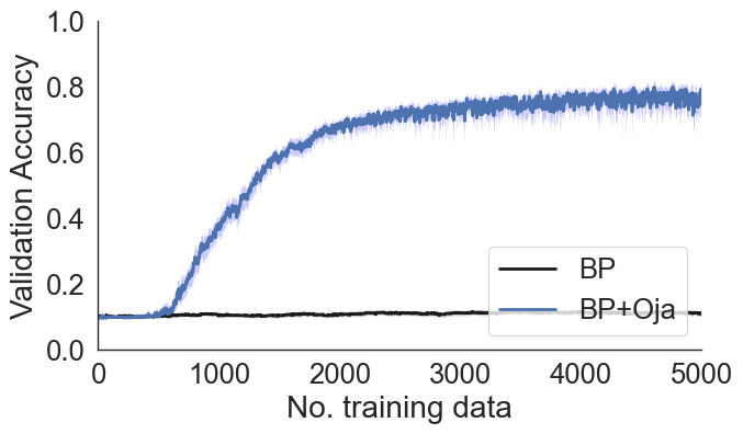
Figure 5: Oja’s rule improves learning in ill-initialized networks. Learning performance comparison on MNIST classification in a 5-layer network with naive weight initialization. The black curve shows the accuracy of a network trained using backpropagation only, while the blue curve shows the accuracy with the addition of Oja’s rule.

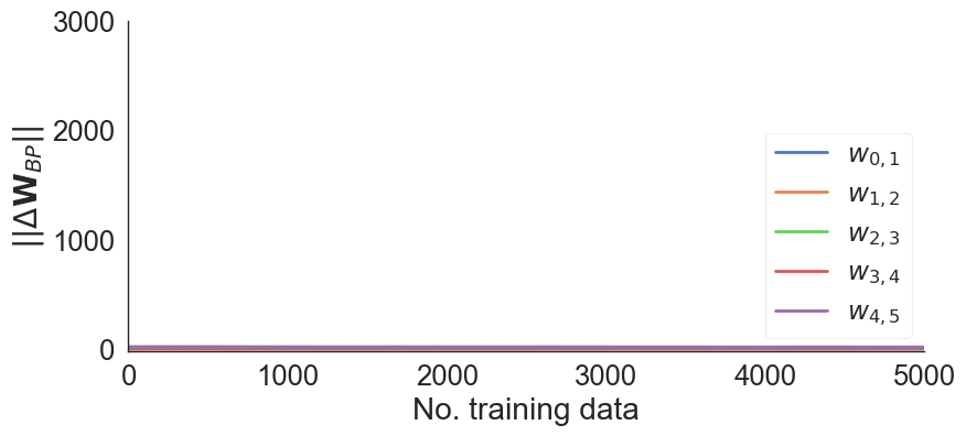
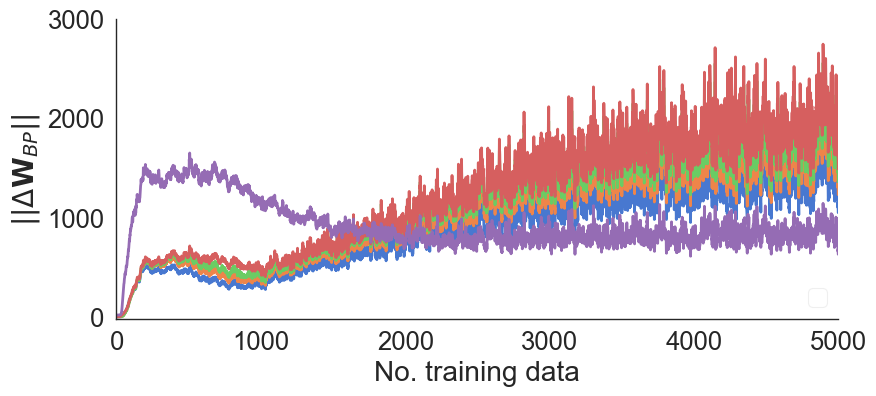
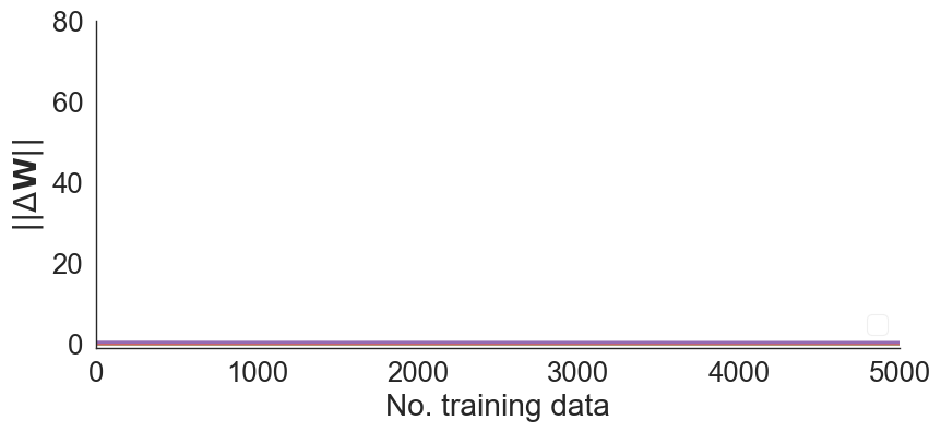
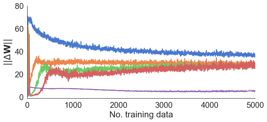
Figure S1: Oja’s rule improves the magnitude of the weight updates in ill-initialized networks. (A) The norm of the backpropagation component ($\|\Delta\boldsymbol{W}_{\text{BP}}\|$) during training for a neural network using standard backpropagation (BP). (B) The norm of the backpropagation component ($\|\Delta\boldsymbol{W}_{\text{BP}}\|$) for a network trained with backpropagation combined with Oja’s rule (BP+Oja). (C) The total weight update norm ($\|\Delta\boldsymbol{W}\|$) for a network using standard BP. (D) The total weight update norm ($\|\Delta\boldsymbol{W}\|$) for a network trained with BP+Oja. The figures on the left show standard BP, while the right figures incorporate Oja’s rule, demonstrating the impact of Oja’s rule on the magnitude of weight updates during training.

This result emphasizes the sensitivity of pure backprop to weight initialization. When weights are initialized with very small values, the gradients during backpropagation are also very small, leading to minimal weight updates and poor learning performance [22] (see Supplementary Fig. S1). In addition, each weight scales the input by a value smaller than one, resulting in a progressively diminishing signal as the network becomes increasingly deep [20].

In contrast, adding Oja’s rule to backpropagation dramatically improved learning performance (Figure 5, blue curve). This result suggests that Oja’s rule can act as a regularizer that dynamically adjusts weights based on activations, compensating for the lack of precise initialization. By implicitly scaling weights during learning, Oja’s rule helps to maintain the flow of information through the network, thereby supporting more stable and effective learning. This result demonstrates that Oja’s plasticity rule provides a biologicaly parsimonious way to overcome the sensitivity of gradient-based learning to weight initialization.

2.3 Comparison to batch normalization

Batch normalization (BN) is a popular methodology for stabilizing activations during neural network training. BN provides stability by directly adjusting activations within the model’s architecture. By comparison, Oja’s rule modifies weights within the optimization process.

BN normalizes activations within mini-batches by standardizing them using batch mean and variance. This process ensurs a stable distribution of the feature maps, resulting in enhanced performance of the model. Nonetheless, the method comes with the cost of additional learnable parameters (mean and variance per dimension for linear layers), which increases the model’s complexity. Moreover, BN depends on batch statistics, making it unsuitable for online learning scenarios.

Conversely, Oja’s rule provides an implicit control on activations by constraining the norm of the weights. This indirect stabilization through the orthonormality constraint imposed by Oja’s rule prevents feature maps from becoming excessively large. For linear transformations $\boldsymbol{z}_{\ell}=\boldsymbol{W}_{\ell-1,\ell}\boldsymbol{y}_{\ell-1}$, orthonormalizing the weight matrix preserves the norm of activations.

$$\|\boldsymbol{z}_{\ell}\|=\sqrt{\boldsymbol{z}_{\ell}^{T}\boldsymbol{z}_{\ell}}=\sqrt{\boldsymbol{y}_{\ell-1}^{T}\boldsymbol{W}_{\ell-1,\ell}^{T}\boldsymbol{W}_{\ell-1,\ell}\boldsymbol{y}_{\ell-1}}=\sqrt{\boldsymbol{y}_{\ell-1}^{T}\boldsymbol{y}_{\ell-1}}=\|\boldsymbol{y}_{\ell-1}\|$$

Our empirical evidence suggests a similar effect in neural networks with non-linearities.

Figure 6: Oja’s rule preserves activation norms across layers. (a) Activation norms in a baseline 5-layer neural network trained with backpropagation (BP) and (b) with BP combined with Oja’s rule (BP+Oja). (c) Activation norms for the same 5-layer network using naive initialization, comparing BP and (d) BP+Oja. (e) Activation norms in a deeper 10-layer network, showing the impact of BP and (f) BP+Oja. (g) Activation norms for a network trained using feedback alignment, a biologically plausible alternative to backpropagation that employs fixed feedback matrices to propagate errors upstream, comparing FA and (h) FA+Oja. Across all configurations, Oja’s rule helps maintain stable activation norms across layers, indicating its role in regularizing neural network training.

While BN does not explicitly fix the norms of activations, it stabilizes them indirectly by normalizing their mean and variance.

2.4 Oja’s rule improves learning of a short term memory task in RNNs

Recurrent Neural Networks (RNNs) are powerful tools for processing sequential data, but their ability to store information over long-term dependencies is hindered by the vanishing and exploding gradient problem [23, 24]. Approaches to mitigate this issue include architectural modifications and optimization improvements. Architectural modifications often involve models that use explicit gating of information flow and memory cells [25]. On the other hand, many optimization-based approaches focus on specific initializations of the model’s recurrent connections, such as unitary [26] or orthogonal matrices [27], as a critical component for the model’s success. While effective, the biological plausibility of these methods are contested [28].

In a vanilla RNN, the recurrent layer dynamics are defined as follows:

$$\mathbf{z}_{t+1}=\boldsymbol{W}_{h}\sigma(\mathbf{z}_{t})+\boldsymbol{W}_{x}\mathbf{x}_{t+1}$$

where $\mathbf{z}_{t}$ represents the hidden state at time step $t$, $\boldsymbol{W}_{h}$ is the recurrent weight matrix, $\sigma$ is a non-linear activation function, $\boldsymbol{W}_{x}$ is the input weight matrix, and $\mathbf{x}_{t}$ is the input at time $t$. We consider a task in which the output is only determined by the final hidden state, so she readout layer for the model is defined by

$$\mathbf{y}_{T}=\boldsymbol{W}_{o}\sigma(\mathbf{z}_{T})$$

Here, $\mathbf{y}_{T}$ represents the output at the final time step $T$, and $\boldsymbol{W}_{o}$ is the readout weight matrix. At each time step, the model combines the previous hidden state and the new input to form the hidden state at the current time step. These model parameters are updated through backpropagation through time (BPTT), which propagates errors back through the unrolled computational graph to update the weights. For recurrent connections, we have

$$\Delta\boldsymbol{W}_{h}=\theta\sum_{t=1}^{T-1}\mathbf{e}_{t+1}\sigma(\mathbf{z}_{t})^{T},$$ (4)

where $\mathbf{e}_{t}$ is the error term propagated back through time

$$\mathbf{e}_{t}=\boldsymbol{W}_{h}^{T}\mathbf{e}_{t+1}\odot\sigma^{\prime}\left(\mathbf{z}_{t}\right),$$ (5)

with $\mathbf{e}_{T}=\partial\mathcal{L}/\partial\mathbf{z}_{T}$ and $\mathcal{L}$ represents the loss.

To enhance the model’s performance, we aim to find a subspace where the projection of the hidden states can be reconstructed with minimal error. While many models attempt to address this with explicit orthogonality constraints [29] or penalty terms [30] to preserve norms, we focus on implicitly preserving the norm during the hidden state transition itself, excluding the new input’s contribution.

In criterion in Eq. 2, we substitute the mapped term with $\boldsymbol{W}_{h}\sigma(\cdot)$ to get

$$\mathcal{J}=\frac{1}{N}\sum_{i=1}^{N}\sum_{t=1}^{T}\|\mathbf{z}_{t}^{(i)}-\boldsymbol{W}_{h}^{T}\boldsymbol{W}_{h}\sigma(\mathbf{z}_{t}^{(i)})\|^{2}.$$ (6)

where $N$ is the number of sequences in the training set.

In our model, we treat the recursive propagation of information similar to a stream of data on the same weight. This forms a non-linear PCA layer on the input data, improving the feature representation of the previous timesteps. At each recurrent iteration, we overlook the contribution of the new input $\mathbf{x}_{t+1}$ to the hidden state, performing Oja’s rule only on the contribution of the hidden state from the previous time step. The update for the weight matrix $\boldsymbol{W}_{h}$ during training can be derived as:

$$\Delta\boldsymbol{W}_{h}=\theta_{1}\sum_{t=1}^{T-1}\mathbf{e}_{t+1}\sigma(\mathbf{z}_{t})^{T}+\theta_{2}\sum_{t=1}^{T-1}\boldsymbol{W}_{h}\sigma(\mathbf{z}_{t})\mathbf{z}_{t}^{T}-\boldsymbol{W}_{h}\sigma(\mathbf{z}_{t})\sigma(\mathbf{z}_{t})^{T}\boldsymbol{W}_{h}^{T}\boldsymbol{W}_{h}$$

We evaluate our model’s ability to memorize and classify handwritten digits using the MNIST dataset subjected to a delay period. The model observes an MNIST image for 5 timesteps. Following a delay period lasting until $T=50$, at which point the model must predict the category of the presented image.

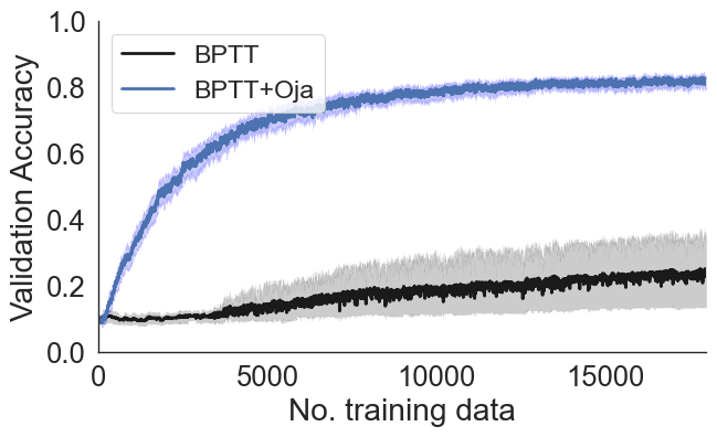
Figure 7: Oja’s rule improves performance in RNNs. Validation accuracy of a Recurrent Neural Network (RNN) trained on the MNIST dataset using Backpropagation Through Time (BPTT) compared with a model using BPTT combined with Oja’s rule (BPTT+Oja). Results demonstrate a substantial improvement in learning efficiency and final accuracy compared to the standard BPTT method.

While increasing the dimension may increase the memory capacity of the model trained with backpropagation, Oja’s rule can improve this even at lower dimensions. Unlike models that impose explicit orthogonality constraints, our update rule implicitly imposes this through the feedback term.

2.5 Oja’s rule improves the performance of networks without explicit weight alignment

In error-based learning, activations are passed forward through the network (Eq. 1) to compute its output while error signals are passed backward through the network

$$\mathbf{e}_{\ell}=\boldsymbol{B}_{\ell+1,\ell}\mathbf{e}_{\ell+1}\odot\sigma^{\prime}(\mathbf{z}_{\ell}),$$ (7)

to modify the weights. However, accurate computation of gradients

$$\frac{\partial\mathcal{L}}{\partial\boldsymbol{W}_{\ell-1,\ell}}=\mathbf{e}_{\ell}\mathbf{y}_{\ell-1}^{T},$$ (8)

needed in gradient-based updates such as backpropagation, requires that the backward projecting weights are symmetric to the forward projecting weights, i.e., $\boldsymbol{B}_{\ell,\ell-1}=\boldsymbol{W}_{\ell-1,\ell}^{T}$. In other words, the forward weight connecting neuron $j$ in layer $\ell$ to neuron $k$ in layer $\ell+1$ has the same value as the backward weight that connects $k$ in layer $\ell+1$ back to neuron $j$ in layer $\ell$. This assumption of precisely symmetric forward and backward weights, known as “weight symmetry,” lacks a biological basis.

Departing from this symmetry, random weight alignment fixes the backward matrix to a randomly initialized value so that backward weights are decoupled from the forward pathway. Under this setting, while the model learns, its performance is severely deteriorated under biologically relevant training setting, such as online learning and small training data sizes [31].

Previous work has shown that various plasticity rules can help align forward and backward weights [32], allowing networks without explicitly aligned weights to approximate the performance of backpropagation. In our previous work [14], we demonstrated that Oja’s rule, when combined with other plasticity rules, can improve the performance of networks without explicitly aligned weights. However, in that work, the networks trained using Oja’s rule only matched, but did not surpass the performance of networks trained using backpropagation with aligned weights.

Notably, in this prior work, we found that Oja’s rule enhances learning performance by improving the flow of information in the forward pathway, rather than directly contributing to the aligning of weights, which was achieved by different plasticity rules. Based on this finding, combined with the success of Oja’s rule in outperforming backpropagation in the scenarios discussed above (Figures 1B, 5, and 7), we hypothesized that combining Oja’s rule with other plasticity rules in a network without explicitly aligned weights could exceed the performance of a network trained using pure backpropagation with aligned weights.

To test this hypothesis, we followed our previous approach [14] to define a plasticity rule as a linear combination of multiple update rules, including an Oja’s subspace term. The update rules are defined as

$$\begin{split}\Delta\boldsymbol{W}_{\ell-1,\ell}=-&\theta_{0}\mathbf{e}_{\ell}\mathbf{y}_{\ell-1}^{T}+\theta_{1}\mathbf{e}_{\ell}\mathbf{e}_{\ell-1}^{T}+\theta_{2}(\mathbf{y}_{\ell}\mathbf{y}_{\ell-1}^{T}-(\mathbf{y}_{\ell}\mathbf{y}_{\ell}^{T})\boldsymbol{W}_{\ell-1,\ell})-\theta_{3}\boldsymbol{W}_{\ell-1,\ell}\\ \Delta\boldsymbol{B}_{\ell,\ell-1}=-&\theta_{4}\mathbf{y}_{\ell}\mathbf{e}_{\ell-1}^{T}+\theta_{9}\boldsymbol{B}_{\ell,\ell-1},\end{split}$$ (9)

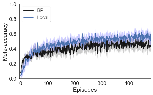
Figure 8: Oja’s rule gives rise to biologically plausible rules that can outperform backpropagation. Meta-accuracy of networks trained with and without explicit weight alignment. This figure compares the meta-accuracy of networks trained using backpropagation (BP) and the local learning rule across multiple episodes. The black curve represents the performance of a network trained using standard backpropagation, while the blue curve shows the performance of a network trained with a local learning rule that does not require explicit weight symmetry (Eq. 9). The meta-accuracy, which measures how well the network generalizes across episodes, increases steadily over time, with the local learning rule consistently outperforming standard backpropagation. This suggests that the local learning rule, that incorporates Oja’s rule, enhances the network’s ability to learn effectively without relying on perfectly aligned weights.

The coefficients, $\theta_{k}$, in the learning rule significantly influence the network’s training dynamics and final performance. Improperly tuned coefficients can lead to suboptimal learning, slower convergence, or instability during training. This is particularly important when more than one plasticity rule is involved, where the interaction between different terms complicates the learning dynamics. In addition, as the number of learning parameters increases, performing a grid search to tune the hyper-parameters becomes exponentially more tedious.

Our previous study developed a meta-learning approach to discover effective plasticity rules that enhance learning performance under biological constraints. We take advantage of this framework to tune the plasticity hyper-parameters. The meta-learning paradigm consists of two optimization loops: an inner adaptation loop and an outer meta-optimization loop. Each meta-iteration, or episode, begins with training a randomly initialized network on a sequence of data points using a candidate plasticity rule. This rule is a parameterized combination of several candidate terms. The loss is computed based on the network’s performance on the training data.

The meta-parameters that define the plasticity rule are updated based on the network’s performance on a separate query set. Meta-optimization aims to minimize meta-loss, which includes a regularization term to encourage sparsity. Hence, it acts as a model selection method to identify the most effective plasticity terms.

3 Discussion

This study explored the effectiveness of Oja’s plasticity rule in overcoming several challenges inherent in training neural networks under biologically plausible conditions. Our work builds on previous research that demonstrated the potential of Oja’s rule to improve the performance of biologically inspired error-based learning to match backpropagation [14]. Here, we extend these findings by showing that incorporating Oja’s rule can help exceed the performance of pure backpropagation. This improvement is particularly evident in challenging learning contexts such as deeper networks, sub-optimal weight initialization, and the absence of batch normalization.

One of the primary differences between this work and previous studies is the novel combination of Oja’s rule with pure backpropagation. This approach allowed us to demonstrate how Oja’s rule can stabilize learning in networks. Oja’s rule proves effective where traditional engineering solutions, such as careful weight initialization and batch normalization, are not viable. Our results show that Oja’s rule can serve as a regularizer, dynamically adjusting weights in response to neural activations. This adjustment helps mitigate the effects of poor initialization and the absence of batch normalization.

Our choice of fully connected layers in this study was strategic, allowing for a straightforward interpretation of plasticity rules under this architecture. Although convolutional layers generally perform better in image classification tasks, they present challenges. Specifically, they make applying and interpreting plasticity rules like Oja’s more difficult due to weight sharing. However, this also opens up exciting future research possibilities. Future work could focus on deriving analogous rules for convolutional and attention layers. This objective could potentially broaden the applicability of Oja’s rule to more complex benchmarks. The constraints of fully connected layers influenced our use of relatively simple datasets like MNIST and FashionMNIST. These datasets allowed us to demonstrate the effects of Oja’s rule without introducing more complex architectures.

Residual connections are a practical solution when considering alternative methods to overcome the training challenges discussed here. They offer a different strategy to maintain the flow of activations and gradients in deep networks [33]. Residual connections are generally seen as biologically plausible. Our findings suggest that Oja’s rule could potentially complement such mechanisms in the brain, working in tandem to stabilize learning.

Our findings underscore the potential of biologically inspired plasticity rules like Oja’s in improving the training of deep networks. These improvements are especially relevant under constraints that are more aligned with biological processes. This work represents an essential step toward developing biologically inspired neural network training methods. These methods depart from the biologically implausible engineering tricks commonly used today.

Supplementary Material

References

- [1] T. P. Lillicrap, A. Santoro, L. Marris, C. J. Akerman, and G. Hinton. Backpropagation and the brain. Nature Reviews Neuroscience, 21(6):335–346, 2020.
- [2] J. C. Whittington and R. Bogacz. Theories of error back-propagation in the brain. Trends in cognitive sciences, 23(3):235–250, 2019.
- [3] T. P. Lillicrap, D. Cownden, D. B. Tweed, and C. J. Akerman. Random synaptic feedback weights support error backpropagation for deep learning. Nature communications, 7(1):1–10, 2016.
- [4] S. Grossberg. Competitive learning: From interactive activation to adaptive resonance. Cognitive science, 11(1):23–63, 1987.
- [5] J. F. Kolen and J. B. Pollack. Backpropagation without weight transport. In Proceedings of 1994 IEEE International Conference on Neural Networks (ICNN’94), volume 3, pages 1375–1380. IEEE, 1994.
- [6] M. Akrout, C. Wilson, P. Humphreys, T. Lillicrap, and D. B. Tweed. Deep learning without weight transport. Advances in neural information processing systems, 32, 2019.
- [7] S. Ioffe and C. Szegedy. Batch normalization: Accelerating deep network training by reducing internal covariate shift. In International conference on machine learning, pages 448–456. PMLR, 2015.
- [8] D. P. Kingma and J. Ba. Adam: A method for stochastic optimization. arXiv preprint arXiv:1412.6980, 2014.
- [9] G. Hinton, N. Srivastava, and K. Swersky. Rmsprop: Divide the gradient by a running average of its recent magnitude. https://www.coursera.org/lecture/neural-networks-deep-learning/lecture-6e-mechanics-of-learning-rmsprop-KdHn, 2012. Coursera: Neural Networks for Machine Learning.
- [10] X. Glorot and Y. Bengio. Understanding the difficulty of training deep feedforward neural networks. In Proceedings of the thirteenth international conference on artificial intelligence and statistics, pages 249–256. JMLR Workshop and Conference Proceedings, 2010.
- [11] J. Barral and A. D Reyes. Synaptic scaling rule preserves excitatory–inhibitory balance and salient neuronal network dynamics. Nature neuroscience, 19(12):1690–1696, 2016.
- [12] M. C. Frank. Bridging the data gap between children and large language models. Trends in Cognitive Sciences, 2023.
- [13] E. Oja. Neural networks, principal components, and subspaces. International journal of neural systems, 1(01):61–68, 1989.
- [14] N. Shervani-Tabar and R. Rosenbaum. “meta-learning biologically plausible plasticity rules with random feedback pathways” metalearning-plasticity repository. Zenodo, doi:10.5281/zenodo.7706619, 2023.
- [15] A. Payeur, J. Guerguiev, F. Zenke, B. A. Richards, and R. Naud. Burst-dependent synaptic plasticity can coordinate learning in hierarchical circuits. Nature neuroscience, 24(7):1010–1019, 2021.
- [16] N. Qian. On the momentum term in gradient descent learning algorithms. Neural networks, 12(1):145–151, 1999.
- [17] E. Oja. Simplified neuron model as a principal component analyzer. Journal of mathematical biology, 15(3):267–273, 1982.
- [18] E. Oja. The nonlinear pca learning rule in independent component analysis. Neurocomputing, 17(1):25–45, 1997.
- [19] N. B. Karayiannis. Accelerating the training of feedforward neural networks using generalized hebbian rules for initializing the internal representations. IEEE transactions on neural networks, 7(2):419–426, 1996.
- [20] K. He, X. Zhang, S. Ren, and J. Sun. Delving deep into rectifiers: Surpassing human-level performance on imagenet classification. In Proceedings of the IEEE international conference on computer vision, pages 1026–1034, 2015.
- [21] A. Krizhevsky, I. Sutskever, and G. E. Hinton. Imagenet classification with deep convolutional neural networks. Advances in neural information processing systems, 25, 2012.
- [22] Y. A. LeCun, L. Bottou, G. B. Orr, and K.-R. Müller. Efficient BackProp, pages 9–48. Springer Berlin Heidelberg, Berlin, Heidelberg, 2012.
- [23] Y. Bengio, P. Simard, and P. Frasconi. Learning long-term dependencies with gradient descent is difficult. IEEE transactions on neural networks, 5(2):157–166, 1994.
- [24] R. Pascanu, T. Mikolov, and Y. Bengio. On the difficulty of training recurrent neural networks. In International conference on machine learning, pages 1310–1318. Pmlr, 2013.
- [25] S. Hochreiter and J. Schmidhuber. Long short-term memory. Neural computation, 9(8):1735–1780, 1997.
- [26] Q. V. Le, N. Jaitly, and G. E. Hinton. A simple way to initialize recurrent networks of rectified linear units. arXiv preprint arXiv:1504.00941, 2015.
- [27] M. Henaff, A. Szlam, and Y. LeCun. Recurrent orthogonal networks and long-memory tasks. In International Conference on Machine Learning, pages 2034–2042. PMLR, 2016.
- [28] R. Costa, I. A. Assael, B. Shillingford, N. De Freitas, and T. Vogels. Cortical microcircuits as gated-recurrent neural networks. Advances in neural information processing systems, 30, 2017.
- [29] E. Vorontsov, C. Trabelsi, S. Kadoury, and C. Pal. On orthogonality and learning recurrent networks with long term dependencies. In International Conference on Machine Learning, pages 3570–3578. PMLR, 2017.
- [30] D. Krueger and R. Memisevic. Regularizing rnns by stabilizing activations. arXiv preprint arXiv:1511.08400, 2015.
- [31] Q. Liao, J. Leibo, and T. Poggio. How important is weight symmetry in backpropagation? In Proceedings of the AAAI Conference on Artificial Intelligence, volume 30, pages 1837–1844, 2016.
- [32] D. Kunin, A. Nayebi, J. Sagastuy-Brena, S. Ganguli, J. Bloom, and D. Yamins. Two routes to scalable credit assignment without weight symmetry. In International Conference on Machine Learning, pages 5511–5521. PMLR, 2020.
- [33] K. He, X. Zhang, S. Ren, and J. Sun. Deep residual learning for image recognition. In Proceedings of the IEEE conference on computer vision and pattern recognition, pages 770–778, 2016.