A controlled-squeeze gate in superconducting quantum circuits

Abstract

We present a method to prepare non-classical states of the electromagnetic field in a microwave resonator. It is based on a controlled gate that applies a squeezing operation on a SQUID-terminated resonator conditioned on the state of a dispersively coupled qubit. This controlled-squeeze gate, when combined with Gaussian operations on the resonator, is universal. We explore the use of this tool to map an arbitrary qubit state into a superposition of squeezed states. In particular, we target a bosonic code with well-defined superparity which makes photon losses detectable by nondemolition parity measurements. We analyze the possibility of implementing this using state-of-the-art circuit QED tools and conclude that it is within reach of current technologies.

Circuit quantum electrodynamics (cQED) has become the leading architecture for quantum computation. In this type of setup one can design different types of qubits using appropriately chosen combinations of Josephson junctions, capacitors, and inductors controlling them with microwave fields Blais et al. (2021); AI (2023); Krinner et al. (2022). Circuit QED has already been used to manipulate tens of qubits for quantum simulation Houck et al. (2012); Andersen et al. (2024) and quantum error correction Reed et al. (2012); goo (2023). Even at the small scale of a few resonators, cQED provides an alternative to Cavity QED Haroche et al. (2020) with practical advantages. It has been used to study the dynamical Casimir effect (DCE) Wilson et al. (2011); Lähteenmäki et al. (2013), foundational aspects of quantum mechanics Devoret et al. (1985); Minev et al. (2019), and also enabled practical applications like error correction of non-classical states in resonators Ofek et al. (2016); Sivak et al. (2023) and quantum communication Storz et al. (2023).

The preparation and control of non-classical quantum states of the electromagnetic field in the resonator is crucial to perform universal simulations which in principle involve the manipulation of arbitrary quantum states. This has a long and interesting history which includes the preparation of quantum superpositions of coherent states (Schrödinger cat states) using field displacement or rotations controlled by the state of the qubit Monroe et al. (1996); Brune et al. (1996); Haroche and Raimond (2006). These studies are not only interesting from the technological point of view but mostly from their fundamental implications and enabled, for example, the first real-time analysis of the process of decoherence in a cavity QED setups Haroche and Raimond (2006); Deleglise et al. (2008).

To generate arbitrary states of the cavity field with limited resources it is crucial to identify a universal set of gates Khaneja et al. (2005); Leghtas et al. (2013); Heeres et al. (2017); Krastanov et al. (2015); Kudra et al. (2022). In this context it has been shown that arbitrary unitary operators acting on the resonator field states can be generated using Gaussian operations together with controlled displacement operators Eickbusch et al. (2022) (which are denoted as $\textbf{C-Dsp}(\gamma)$ and applies a displacement $\hat{D}(\gamma)$ depending on the state of a control qubit). Complemented with Gaussian operations on the field, this controlled-gate provides a universal resource to create arbitrary states.

In this letter we present another gate, based on controlled squeezing, that provides a universal resource, and show that it demands reasonable experimental resources. We will denote it as $\textbf{C-Sqz}(r,\theta)$ as it applies the squeezing operation $\hat{S}(r,\theta)$, conditioned on the state of a control qubit. We also present an example protocol to make use of this gate in cQED setup to encode quantum states in the resonator using an encoding that makes the errors induced by the loss of a photon detectable through parity measurement. But before going into this we prove here the universality of the controlled-squeeze gate as follows. The squeezing operator $\hat{S}(r,\theta)$, is defined as $\hat{S}(r,\theta)=\exp(r/2(e^{-i\theta}\hat{a}^{2}-e^{i\theta}\hat{a}^{\dagger 2}))$ and satisfies the following simple property when combined with the displacement operation $\hat{D}(\gamma)$: $\hat{S}(r,\theta)\hat{D}(\gamma)\hat{S}^{-1}(r,\theta)=\hat{D}(\gamma^{\prime})$ with $\gamma^{\prime}=\gamma\cosh r-\gamma^{*}e^{i\theta}\sinh r$. That is to say that applying the displacement $\hat{D}(\gamma)$ in between $\hat{S}^{-1}(r,\theta)$ and $\hat{S}(r,\theta)$ is equivalent to the application of a different displacement $\hat{D}(\gamma^{\prime})$, an idea that was used by Wineland and co-workers to build a motional amplifier using an amplitude modulated ion trap to generate squeezing Wineland (2013). The above relation between squeezing and displacement operators can be simply generalized to the case of control gates by showing that $\hat{D}^{-1}(\gamma)\textbf{C-Sqz}(r,\theta)\hat{D}(\gamma)(\textbf{C-Sqz})^{-1}(r,\theta)=\textbf{C-Dsp}(\gamma^{\prime}-\gamma)$. Therefore the use of an arbitrary $\textbf{C-Sqz}(r,\theta)$ gate together with a fixed displacement operator would enable the implementation of arbitrary control displacement. Thus the universality of $\textbf{C-Dsp}(\gamma)$ implies the universality of $\textbf{C-Sqz}(r,\theta)$. Choosing a universal set of gates over others is a decision that should be made considering the hardware at hand and the target states or operators desired. Our proposal enables the implementation of controlled displacements and controlled squeezing gates in the same setup, and therefore adds flexibility to the cQED architecture, simplifying certain tasks.

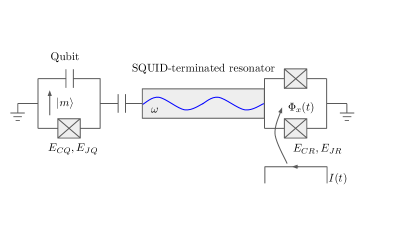
Figure 1: The setup proposed consists of a coplanar wave guide acting as a resonator and terminated in a SQUID at the right end and capacitively coupled to a transmon at the left. The SQUID is used to parametrically drive the resonator by applying a time dependent magnetic flux to it. The transmon qubit is initially prepared in a quantum state $|m\rangle$ (where $m=0,1$) and acts as a switch that either tunes or detunes the resonator to the driving frequency.

To implement the proposed controlled-squeeze gate we use two basic elements: one frequency-tunable resonator and a qubit Paik et al. (2011); Wang et al. (2022) with quantum states $|0\rangle$ and $|1\rangle$. This qubit is dispersively coupled to the resonator in the number splitting regime, so that its frequency depends of the state of the qubit (i.e. it is $\bar{\omega}_{0}$ if the state is $|0\rangle$ and $\bar{\omega}_{1}$ if the state is $|1\rangle$). The resonator is terminated by a SQUID, where we apply a time-dependent flux $\Phi(t)=\epsilon\sin(\omega_{d}t)$. In this way the resonator’s natural frequency becomes a time-dependent parameter $\omega_{0,1}(t)=\bar{\omega}_{0,1}+g_{d}\epsilon\sin(\omega_{d}t-\theta)$, where $g_{d}$ is the driving coupling constant between the SQUID and the resonator modes (see below) and $\epsilon$ is the amplitude of the flux drive. When the driving frequency is $\omega_{d}=2\bar{\omega}_{1}$, then parametric resonance takes place and the cavity’s field is squeezed as a result Wu et al. (1987). If the detuning $\Delta=\bar{\omega}_{1}-\bar{\omega}_{0}$ is $\Delta\gg g_{d}\epsilon$ then the state of the cavity field is effectively squeezed only if the control qubit is in the state $|1\rangle$. On the other hand, if the state is $|0\rangle$, ordinary harmonic evolution with frequency $\bar{\omega}_{0}$ takes place and when compensated as described below, turns this into a controlled-squeeze gate.

The setup we envision is described in Fig. 1: the transmon qubit in the left is capacitively coupled with a $\lambda/4$ resonator terminated by a flux-tunable SQUID. This last component has been used to demonstrate the dynamical Casimir effect Svensson et al. (2018); Wilson et al. (2010), and has been the subject of thorough investigation Wustmann and Shumeiko (2013); Johansson et al. (2010). The setup in Fig. 1 can be modeled with the Hamiltonian (we use $\hbar=1$ thorough the letter)

$$\hat{H}(t)=\frac{\omega_{q}}{2}\hat{\sigma}_{z}+\omega\hat{a}^{\dagger}\hat{a}+\chi\hat{a}^{\dagger}\hat{a}\hat{\sigma}_{z}+g_{d}\epsilon\sin(\omega_{d}t-\theta)(\hat{a}^{\dagger}+\hat{a})^{2},$$ (1)

where $\hat{a}$ is the bosonic annihilation operator of the resonator mode and $\hat{\sigma}_{z}=|0\rangle\langle 0|-|1\rangle\langle 1|$ is the Pauli operator associated with the qubit. Here, $\omega_{q}$ is the frequency of the qubit, and $\chi$ is the dispersive coupling constant between the resonator and the transmon. The dependence of these constants on physically relevant parameters such as the Josephson energy, the capacitance of the transmon-qubit, its charge energy, the coupling capacitance, the inductance and capacitance per unit length of the resonator and the parameters characterizing the external pumping are discussed in detail in the Supplemental Material SM . The Hamiltonian in (1) does not include non-linearities, which as discussed in the Supplemental Material SM , can be neglected when the ratio between the Josephson energy of the SQUID in the right and the inductive energy of the resonator ($E_{L,{\rm res}}/E_{J}$) is small. In what follows we will work under this assumption and explain the effect of the Hamiltonian (1), presenting later some results with experimentally realizable parameters discussing also the effect of losses, decoherence, and non-linearities. A similar Hamiltonian appears in the context of trapped ions where a gate that squeezes the motional degree of freedom of an ion depending on its internal state was proposed by modulating the amplitude of an optical lattice Drechsler et al. (2020).

By looking at the Hamiltonian in Eq. (1) one can see that it describes a harmonic oscillator with a resonance frequency $\omega_{0,1}(t)$ that both varies in time and is conditioned on the qubit state ($\bar{\omega}_{0}=\omega+\chi$ when the qubit is in the state $|0\rangle$ or $\bar{\omega}_{1}=\omega-\chi$ when the qubit is in the state $|1\rangle$). If the system is driven with $\omega_{d}=2\bar{\omega}_{1}$, and the qubit state is $|1\rangle$, then the parametric resonance is exited and the state of the resonator is squeezed. On the other hand, if the state of the qubit is $|0\rangle$, the resonator simple acquires a renormalized frequency due to the effect of the AC-Stark shift. Thus, in the frame rotating with frequency $\bar{\omega}_{1}$, the Hamiltonian (1), within the rotating wave approximation (RWA), reads as (see Supplemental Material SM )

$$\hat{H}_{I}=\frac{1}{2}ig_{d}\epsilon(e^{-i\theta}\hat{a}^{2}-e^{i\theta}\hat{a}^{\dagger 2})\otimes|1\rangle\langle 1|+\tilde{\Delta}\hat{a}^{\dagger}\hat{a}\otimes|0\rangle\langle 0|,$$ (2)

where $\tilde{\Delta}\approx\Delta(1-1/2(g_{d}\epsilon/\Delta)^{2})+{\cal O}((g_{d}\epsilon/\Delta)^{4})$.

The temporal evolution operator associated with the above Hamiltonian is

$$\exp(-i\hat{H}_{I}t) = \hat{S}(r,\theta)\otimes|1\rangle\langle 1|+\hat{U}_{0}(\varphi)\otimes|0\rangle\langle 0|$$ (3)

$$= \hat{U}(r,\theta,\varphi),$$

where $\hat{S}(r,\theta)$ is the squeezing operator defined above, with the squeezing parameter $r=-g_{d}\epsilon t$ and the squeezing angle $\theta$ set by the phase of the driving. Above, $\hat{U}_{0}(\varphi)$ is the evolution operator of an oscillator with frequency $\tilde{\Delta}$, which during a time $t$, induces a rotation in phase space in an angle $\varphi=\tilde{\Delta}t$. For the above evolution operator $\hat{U}(r,\theta,\varphi)$ in Eq.(3) to be a true controlled-squeeze gate, it is necessary to compensate the free evolution $\hat{U}_{0}(\varphi)$. This can be done, at least in two different ways. First, one can turn off the magnetic driving and then wait a time $\tau$ chosen in such a way that $\Delta\tau+\varphi=2k\pi$, for some integer $k$. After this, as $\hat{U}_{0}(\Delta\tau)\hat{U}_{0}(\varphi)=1$, the evolution operator is the desired controlled-squeeze gate: $\textbf{C-Sqz}(r,\theta)=\hat{U}_{0}(\Delta\tau)\otimes|0\rangle\langle 0|\otimes\hat{U}(r,\theta,\varphi)$. A different alternative, that’s not require turning off the magnetic driving, is to use the non-compensated controlled-squeeze gate $\hat{U}(r,\theta,\varphi)$ and to choose the subsequent operations to depend on the rotation angle $\varphi$. We will follow this second strategy below.

Now we show how to use the above result in order to encode an arbitrary qubit state in a resonator making the errors induced by photons losses detectable Ofek et al. (2016); Ni et al. (2023); Grimsmo et al. (2020); Teoh et al. (2023). We choose the encoding in such a way that the logical states $|0\rangle$ and $|1\rangle$ are represented by the states $|\chi_{+}\rangle$ and $|\chi_{-}\rangle$ of the resonator built as even and odd superposition of states squeezed along two orthogonal directions in quadrature space, i.e.,

$$|\chi_{\pm}\rangle=\frac{1}{\sqrt{2}c_{\pm}}(|r,\tilde{\theta}\rangle\pm|r,\tilde{\theta}+\pi\rangle),$$ (4)

where $|r,\tilde{\theta}\rangle$ is a one-mode squeezed state and the constant $c_{\pm}=\sqrt{1\pm 1/\sqrt{\cosh 2r}}$. From this it is simple to see that the states $|\chi_{+}\rangle$ and $|\chi_{-}\rangle$ have similar properties to the four-legged cat Ofek et al. (2016) states as they are respectively superposition of $4n$ and $4n+2$ photon states, which implies that when loosing a photon the encoded state still stores a coherent superposition and the error can be detected by a subsequent parity measurement of the photon number inside the resonator.

To prepare a general encoded state we should start with an arbitrary qubit state $|\Psi_{Q}\rangle=\alpha|0\rangle+\beta|1\rangle$ and the resonator in the vacuum. Then we apply the following sequence: i) Apply a Hadamard gate to the qubit (transforming $|0\rangle\to(|0\rangle+|1\rangle)/\sqrt{2}$ and $|1\rangle\to(|0\rangle-|1\rangle)/\sqrt{2}$); ii) Apply the non-compensated controlled-squeeze gate $\hat{U}(r,\theta,\varphi)$ defined in Eq.(3); iii) Apply a $\pi$-rotation to the qubit; iv) Apply the operator $\hat{U}(r,\theta+2\varphi+\pi,\varphi)$; v) Apply a $\pi$-rotation to the qubit; and vi) Apply another Hadamard gate to the qubit. After this sequence the combined qubit-resonator state will be

$$|\Psi_{QR}\rangle = \frac{1}{\sqrt{2}}|0\rangle\left(\alpha\ {c}_{+}|\chi_{+}\rangle+\beta\ {c}_{-}|\chi_{-}\rangle\right)$$ (5)

$$+ \frac{1}{\sqrt{2}}|1\rangle\left(\alpha\ {c}_{-}|\chi_{-}\rangle+\beta\ {c}_{+}|\chi_{+}\rangle\right)$$

where $|\chi_{+}\rangle$ and $|\chi_{-}\rangle$ are the above defined ones with $\tilde{\theta}=\theta+2\varphi$. If we measure $\hat{\sigma}_{z}$ for the qubit, we obtain the results $\pm 1$, which respectively identify the states $|0\rangle$ or $|1\rangle$, with probability $P_{\pm}=1/2(1\pm P_{z}/\sqrt{\cosh(2r)})$, where $P_{z}=\alpha^{2}-\beta^{2}$ is the z-component of the polarization vector of the qubit which identifies its state in the Bloch sphere. For each result, the state of the resonator turns out to be $|\Psi_{R}^{\pm}\rangle=(\alpha{c}_{\pm}|\chi_{\pm}\rangle+\beta{c}_{\mp}|\chi_{\mp}\rangle)/\sqrt{|\alpha|^{2}c_{\pm}^{2}+|\beta|^{2}c_{\mp}^{2}}$. For each result $\sigma_{z}=\pm 1$ the resonator stores the encoded states $|\Psi_{R}^{\pm}\rangle$ whose fidelity with respect to ideal state $|\tilde{\Psi}_{Q}^{\pm}\rangle=\alpha|\chi_{\pm}\rangle+\beta|\chi_{\mp}\rangle$ is $F_{\pm}=|\langle\tilde{\Psi}_{Q}^{\pm}|\Psi_{R}^{\pm}\rangle|^{2}$. The average fidelity for the complete encoding protocol is $\bar{F}=P_{+}F_{+}+P_{-}F_{-}$ which can be expressed as

$$\bar{F}=\frac{1}{2}(1+P_{z}^{2})+\frac{1}{2}(1-P_{z}^{2})\sqrt{1-\frac{1}{\cosh(2r)}}.$$ (6)

The lowest fidelity states are those in the equator, i.e. when $P_{z}=0$, and, in the limit of high squeezing, we find that $\bar{F}\sim 1-e^{-2r}(1-P_{z}^{2})/4$. Clearly to enforce a high fidelity for every state we need the squeezing factor to be large enough. In fact $\bar{F}\geq 0.995$ requires $r\geq 2$.

We analyzed the implementation of the above encoding protocol considering material properties that have been achieved in systems similar to the one proposed Eriksson et al. (2024); Ganjam et al. (2024). For this we choose the resonator frequency $\omega/(2\pi)=6\text{GHz}$, the qubit frequency $\omega_{q}/(2\pi)=4\text{GHz}$, the driving coupling $g_{d}=50\text{MHz}$, the driving amplitude $\epsilon=0.15$ and the qubit coupling strength $\chi/(2\pi)=8\text{MHz}$. The controlled-squeeze gate is applied during $200\rm n\text{s}$ resulting in a squeezing $r\sim 1.5$.

We included the effect of losses and decoherence modeled through a master equation describing thermal contact between the qubit-resonator system and a bath at $60\text{mK}$. For the relaxation time-scales we choose values which lying in between the ones reported in Ref. Eriksson et al. (2024) and the most recent one Ganjam et al. (2024): a qubit relaxation time-scale $\tau_{q}=200\mu\text{s}$, a resonator damping time $\tau_{r}=200\mu\text{s}$ and a qubit dephasing time-scale of $\tau_{\phi}=10\mu\text{s}$ (this is also detailed in the Supplemental Material SM ).

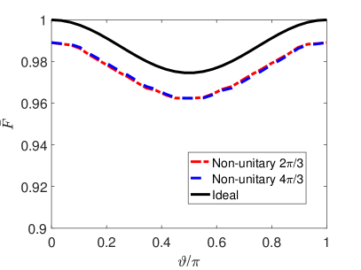
Figure 2: Average fidelity for encoding a qubit state into the resonator as a function of azimutal angle $\vartheta$ of the Bloch sphere for two different values of polar angle $\phi=2\pi/3$ and $4\pi/3$. Physical parameters are: $\omega/(2\pi)=6\text{GHz}$; $\omega_{q}/(2\pi)=4\text{GHz}$; $g_{d}=50\text{MHz}$; $\epsilon=0.15$; and $\chi/(2\pi)=8\text{MHz}$. The qubit and resonator relaxation time-scales are $\tau_{q}=\tau_{r}=200\mu\text{s}$, while the qubit dephasing time is $\tau_{\phi}=10\mu\text{s}$. Coupling with the thermal bath at $60\text{mK}$ was assumed. Upper solid (black) line corresponds to the ideal case of Eq.(6) where coupling to the environment is ignored and the optimization process is not taken into account. Dashed (blue) and dot-dashed (red) lines lie $1\%$ below the unitary line because of the degradation due to the coupling to the environment.

Including non-linearities, losses, and decoherence, we studied the average fidelity and purity decay for arbitrary states in Fig. 2, where the dependence of these quantities with the azimutal angle $\vartheta$ is shown for two typical values of the polar $\phi$-angle in the Bloch sphere. For the above parameters we find, see Fig. 2, average fidelity between $96.2\%$ (for the states in the equator) and $98.9\%$ (for states in both poles of the Bloch sphere). Upper solid line (in black) corresponds to the ideal average fidelity given by Eq.(6) where dissipation and dephasing are not considered. In this case, the obtained values are $1\%$ higher than those arising from numerical simulations that include losses, decoherence, and non-linearities. Purity ranges between $97.3\%$ (in the equator) and $99.3\%$ (in the poles).

For these parameters the analytic estimation of the rotation angle $\varphi$ appearing in the evolution operator in Eq.(3) is $\varphi=20.05$ which is the sum of $\Delta t=20.1$ and the contribution from the dynamical AC-Stark shift given by $1/2\Delta t(g_{d}\epsilon/\Delta)^{2}=-0.05$. To obtain a better quality gate the angle $\varphi$ to be compensated can be numerically estimated using an optimization algorithm to maximize the fidelity after the sequence of the operations described above. With this procedure we find that the best value $\varphi=19.98$ which is very close to the above analytic estimation.

The imperfection in the compensation angle introduces a systematic error in the gate that is very small. Thus, the maximum achievable fidelity in the absent of loses and decoherence in the equator for the squeezing parameter $r=1.5$ is $97\%$ (while it would be $97.5\%$ for the perfect unitary controlled-squeeze gate).

Conclusions. We proposed the use of a controlled-squeeze gate in a cQED. This is a universal gate when combined with Gaussian operations on the resonator state and single-qubit unitaries. We discussed how to use it to encode quantum states initially stored in the qubit mapping them onto resonator states which are superpositions of $4n$ or $4n+2$ photon states making therefore photon losses detectable by simple parity measurements.

Acknowledgments. This research of NDG, PIV, FCL, and JPP was funded by Agencia Nacional de Promocion Científica y Tecnológica (ANPCyT), Consejo Nacional de Investigaciones Cientıficas y Técnicas (CONICET), and Universidad de Buenos Aires (UBA). RGC acknowledges support from the Yale Quantum Institute.

Supplemental material for ”A controlled-squeeze gate in superconducting quantum circuits”

In this Supplemental Material (SM) we will show how to derive, within the framework of cQED, the Hamiltonian used to describe the SQUID-terminated superconducting resonator. After that, we will show the master equation by which we test our protocol under realistic conditions of dissipation, relaxation and dephasing. The SM ends with the details of the encoding protocol and how to deal with a non-ideal C-Sqz gate.

Appendix A Hamiltonian for a SQUID terminated resonator

In this Supplemental Material we will show how to derive, using the main ingredients of cQED theory, the Hamiltonian used to describe the SQUID-terminated superconducting resonator. In order to do this we will start from the classical Lagrangian of the composite system, obtain the Hamiltonian for the modes and finally quantize them. We set units with $\hbar=1$, and therefore the quantum magnetic flux $\Phi_{0}=2\pi/(2e)$.

A.1 Lagrangian formulation

We start our derivation with the Lagrangian for the dimensionless phase field $\Phi(x,t)$ inside a superconducting resonator of length $d$ with inductance $L_{0}$ and capacitance $C_{0}$ per unit length, terminated in a SQUID at $x=d$ Wustmann and Shumeiko (2013). This Lagrangian is simply the sum of the one corresponding to the transmission line which occupies the interval $0\leq x<d$ and the one of the SQUID located at $x=d$:

$$L=\left(\frac{1}{2e}\right)^{2}\frac{C_{0}}{2}\int_{0}^{d}(\dot{\Phi}^{2}-v^{2}\Phi^{\prime 2})dx+\left(\frac{1}{2e}\right)^{2}2C_{J}\int_{0}^{d}\frac{\dot{\Phi}^{2}}{2}\delta(x-d)dx+2E_{J}\int_{0}^{d}\cos(\Phi)\cos\left(2e\phi(t)\right)\delta(x-d)dx.$$ (7)

Here $v=1/\sqrt{L_{0}C_{0}}$ is the speed at which the wave propagate in the resonator, whereas $\phi(t)$ is the external magnetic field flux applied to the SQUID. It is worth noticing that term concentrated in $x=d$ enables the derivation of the equations for the phase $\Phi_{d}$ for symmetric SQUIDS, with two identical Josephson junctions, each with Josephson energy $E_{J}$ and capacitance $C_{J}$. In what follows we will use the notation $\Phi_{d}(t)=\Phi(d,t)$.

Evaluating the Euler-Lagrange equation for $\Phi(x,t)$, we obtain

$$\ddot{\Phi}-v^{2}\Phi^{\prime\prime}+\left(\frac{1}{2e}\right)^{2}2C_{J}\ddot{\Phi}_{d}+2E_{J}\cos\left(2e\phi(t)\right)\sin(\Phi_{d})=0.$$ (8)

Evaluating previous equation for $x<d$, one obtains the wave equation for the phase field,

$$\ddot{\Phi}-v^{2}\Phi^{\prime\prime}=0.$$ (9)

The equation for $\Phi_{d}(t)$ can be obtained after integrating Eq. (8) in the spatial coordinate, between $d-\epsilon$ and $d+\epsilon$, for $\epsilon\rightarrow 0$. While doing this, one has to take into account the existence of a discontinuity in the first spatial derivative of $\Phi(x,t)$ at $x=d$. Thus, the equation for the phase field at the position of the SQUID reads as:

$$\left(\frac{1}{2e}\right)^{2}2C_{J}\ddot{\Phi}_{d}+2E_{J}\cos\left(2e\phi(t)\right)\sin(\Phi_{d})+\left(\frac{1}{2e}\right)^{2}C_{0}v^{2}\Phi^{\prime}_{d}=0.$$ (10)

The last two equations along with the Neumann boundary condition at $x=0$, $(\partial_{x}\Phi)(0,t)=0$, define completely the field for the SQUID-terminated resonator.

In order to solve the above equations we first assume the validity of a linear approximation for the phase field $\Phi$ ($\Phi\ll 1$), and take into account non-linearities in a perturbative way later. In this case, when the external flux is constant $\phi(t)=\bar{\phi}$ a basis of solutions for the above equations can be found:

$$\Phi(x,t)=e^{i\omega_{n}t}\psi_{n}(x)$$ (11)

$$\psi_{n}(x)=\frac{1}{N_{n}}\cos(k_{n}x),$$ (12)

where $N_{n}$ is a normalization constant. For these modes to satisfy the wave equation (9), the frequency $\omega_{n}$ must be such that $\omega_{n}^{2}=k_{n}^{2}v^{2}$ is the angular frequency for the modes. Moreover, the equation (10) for $\Phi_{d}$ is satisfied only if the wave number $k_{n}$ satisfy the following transcendental equation:

$$\left(\frac{1}{2e}\right)^{2}C_{0}v^{2}k_{n}\tan(k_{n}d)=2E_{J}\cos\left(2e\bar{\phi}\right)-\left(\frac{1}{2e}\right)^{2}2C_{J}v^{2}k_{n}^{2}.$$ (13)

This transcendental equation uniquely determines the spectrum of the SQUID-terminated resonator $\omega_{n}$ for a given external magnetic flux $\bar{\phi}$.

It is important to stress that the above spatial modes are orthonormal in the following internal product

$$\langle\psi_{i},\psi_{j}\rangle=\int_{0}^{d}\epsilon(x)\psi_{i}(x)\psi_{j}(x)dx,$$ (14)

where $\epsilon(x)=\left(\frac{1}{2e}\right)^{2}C_{0}+\left(\frac{1}{2e}\right)^{2}2C_{J}\delta(x-d)$.

We now analyze the system for a time-dependent magnetic flux $\phi(t)=\bar{\phi}+\delta\phi(t)$ that oscillates around a constant value $\bar{\phi}$. In this case we can define spatial modes $\psi_{n}(t,x)$ with an explicit time dependence arising from the dependence of $k_{n}$ on time through the generalization of the transcendental Eq. (13) to the time dependent case. This new basis (which defines the instantaneous spatial modes) is orthonormal in the same inner product defined above. Using this ansatz for the spatial modes, the phase field can be expanded as

$$\Phi(x,t)=\sum_{n}Q_{n}(t)\psi_{n}(t,x),$$ (15)

where the amplitudes $Q_{n}(t)$ are time dependent functions that contain all the dynamical information of the problem. Clearly, in this basis $\dot{\Phi}(x,t)=\sum_{n}(Q_{n}(t)\dot{\psi}_{n}(t,x)+\dot{Q}_{n}(t)\psi_{n}(t,x))$ and therefore we may evaluate,

$$\frac{1}{2}\int_{0}^{d}dx\,\epsilon(x)\,\dot{\Phi}^{2}=\frac{1}{2}\sum_{k}\dot{Q}_{k}^{2}+\frac{1}{2}\sum_{kj}S_{kj}Q_{k}Q_{j}-\sum_{kj}A_{kj}\dot{Q}_{k}Q_{j},$$ (16)

where

$$S_{kj} = \langle\dot{\psi}_{k},\dot{\psi}_{j}\rangle=\int_{0}^{d}dx\,\epsilon(x)\,\dot{\psi}_{k}\,\dot{\psi}_{j},$$

$$A_{kj} = \langle\psi_{k},\dot{\psi}_{j}\rangle=\int_{0}^{d}dx\,\epsilon(x)\,\psi_{k}\,\dot{\psi}_{j}.$$

Note that, due to the orthogonality of the eigenfunctions, the matrix $A_{kj}$ is antisymmetric. The matrix $S_{kj}$ is obviously symmetric. They ($A_{ij}$ and $S_{ij})$ are, in short, coupling functions that depend on time.

A similar calculation can be done for the spatial derivatives (for details on a related calculation see the appendix of Ref. Fosco et al. (2013))

$$\int_{0}^{d}dx\,\Phi^{\prime 2}=\sum_{kj}Q_{k}\,Q_{j}\int_{0}^{d}dx\,\psi_{k}^{\prime}\,\psi_{j}^{\prime}=\sum_{kj}Q_{k}\,Q_{j}\int_{0}^{d}dx\left[\left(\psi_{k}\psi_{j}^{\prime}\right)^{\prime}-\psi_{k}\psi_{j}^{{}^{\prime\prime}}\right]=\sum_{kj}Q_{k}\,Q_{j}\int_{0}^{d}dx\left[\left(\psi_{k}\psi_{j}^{\prime}\right)^{\prime}+k_{j}^{2}\psi_{k}\psi_{j}\right],$$ (18)

where we have used the wave equation in the last term. It is worth noticing that because the discontinuity at $x=d$, the transcendental equation implies the following relation

$$\int_{0}^{d}dx\left(\psi_{k}\psi_{j}^{\prime}\right)^{\prime}=\left(\frac{2C_{J}}{C_{0}}k_{j}^{2}-\frac{1}{(2e)^{2}}\frac{2E_{J}\cos(2e\phi(t))}{C_{0}v^{2}}\right)\psi_{k}(d)\psi_{j}(d),$$ (19)

that, when combined with Eq. (18), it allows us to cancel those terms that appear in the Lagrangian (7), located at $x=d$.

Therefore, using the orthogonality of the instantaneous modes $\psi_{n}(t,x)$, defined above, we obtain a Lagrangian for the coefficients $Q_{n}(t)$ (which play the role of the generalized coordinates for this problem),

$$L=\frac{1}{2}\sum_{i}\left(\dot{Q_{i}}^{2}-\omega_{i}^{2}Q_{i}^{2}\right)-\sum_{i,j}A_{ij}\dot{Q_{i}}Q_{j}+\sum_{i,j}S_{ij}Q_{i}Q_{j},$$ (20)

where the frequency in the last equation is time dependent through: $\omega_{i}=\omega_{i}(\phi(t))=vk_{i}(\phi(t))$ (and $k_{i}(t)$ are the solutions of the transcendental equation).

A.2 Hamiltonian formulation

From the Lagrangian above (Eq.(20)), the classical Hamiltonian can be found by first calculating the canonical conjugated momenta

$$P_{i}=\frac{\partial L}{\partial\dot{Q}_{i}}=\dot{Q_{i}}-\dot{\delta\phi}\sum_{k}M_{ik}Q_{k},$$ (21)

where we have used that $\dot{\psi}_{k}=d\phi_{k}/d\phi(t)\,\dot{\delta\phi}$ and therefore we can write $A_{ik}=\dot{\delta\phi}\,M_{ik}$ with $M_{ik}=\langle\psi_{i},d\psi_{k}/d\phi\rangle$. Thus, we can write the new coordinates as,

$$\dot{Q_{i}}=P_{i}+\dot{\delta\phi}\sum_{k}M_{ik}Q_{k},$$ (22)

and then, after the Legendre transformation, it is possible to write a Hamiltonian:

$$H=\sum_{i}P_{i}\dot{Q}_{i}-L=\frac{1}{2}\sum_{i}\left[P_{i}^{2}+\omega_{i}^{2}Q_{i}^{2}\right]+\dot{\delta\phi}\sum_{i,k}M_{ik}P_{i}Q_{k}.$$ (23)

We can now proceed to quantize the theory by promoting the generalized coordinates and momenta to operators acting on a Hilbert space with canonical commutation rules

$$[Q_{k},P_{j}]=i\delta_{kj}.$$ (24)

We can also define annihilation operators as

$${\tilde{a}}_{k}=\sqrt{\frac{1}{2{\tilde{\omega}}_{k}(\phi)}}({\tilde{\omega}}_{k}(\phi)Q_{k}+iP_{k}),$$ (25)

which will satisfy the commutation relation $[{\tilde{a}}_{k},{\tilde{a}}_{k}^{\dagger}]=1$.

Assuming the system is weakly driven, i.e., $|\delta\phi(t)|<<1$, the annihilation operators can be approximated by

$${\tilde{a}}_{k}\approx a_{k}+\delta\phi\frac{\omega_{k}^{\prime}}{2\omega_{k}}a_{k}^{\dagger},$$ (26)

where the annihilation operators correspond to the excitations of the static resonator and $\omega_{k}^{\prime}=(d\omega_{k}/d\phi)(\bar{\phi})$. Finally, replacing these results in Eq.(23) we reach to the quantum Hamiltonian

$$H=\sum_{k}\left[\omega_{k}a_{k}^{\dagger}a_{k}+\frac{\omega_{k}^{\prime}}{2}\delta\phi(a_{k}+a_{k}^{\dagger})^{2}\right]+\delta\dot{\phi}\sum_{i,k}\frac{M_{ik}}{2i}\sqrt{\frac{\omega_{i}}{\omega_{k}}}\left(a_{i}a_{k}-a_{i}^{\dagger}a_{k}+a_{i}a_{k}^{\dagger}-a_{i}^{\dagger}a_{k}^{\dagger}\right),$$ (27)

where $M_{ij}$ are now coupling constants that depend only on $\bar{\phi}$. Here, we have neglected the term associated the Kerr effect induced by the SQUID, $K_{\rm SQUID}(a^{\dagger}a^{\dagger}aa)/2$, since we are working under the assumption that the inductive energy of the resonator is much smaller than the Josephson energy of the SQUID, i.e., $\sigma=E_{\rm L,res}/(2E_{J}\cos\left(2e\phi\right))\sim 10^{-2}$ (where $E_{\rm L,res}=(1/2e)^{2}(1/L_{0}d)$) which, as shown in Wustmann and Shumeiko (2013), guarantees that

$$K_{\rm SQUID}/\omega_{k}\approx\sigma^{3}\frac{\pi Z_{0}}{2R_{q}}\leq 10^{-5},$$ (28)

where $Z_{0}=\sqrt{L_{0}/C_{0}}$ is the cavity impedance and $R_{q}=1/(2e^{2})$ is the resistance quantum. In other words, under these assumptions, the coefficient associated with the Kerr effect is negligible.

Finally, the Hamiltonian of Eq.(1) employed in the letter is simply the one-mode approximation of Eq. (27) capacitively coupled to a qubit in the dispersive regime Blais et al. (2021). More precisely, we are assuming that the resonator-transmon coupling constant $g_{q}$, is much smaller than the detuning, $\Delta_{q}=\omega_{q}-\omega$, making the induced Kerr non-linearity negligible

$$K_{\rm qubit}/\omega=-\frac{1}{2}E_{C,q}\left(\frac{g_{q}}{\Delta_{q}}\right)^{4}\sim 10^{-8},$$ (29)

where $g_{q}=\sqrt{-\chi\Delta_{q}(\Delta_{q}-E_{C,q})/E_{C,q}}$ is the qubit-resonator coupling constant and $E_{C,q}=150{\rm MHz}$ is the capacitive energy of the qubit.

Appendix B Master equation

To evaluate the effect of dissipation on the protocol proposed under experimental conditions we adopt a master equation approach. The state of the joint system, resonator plus qubit, is then described by a density matrix. Taking a harmonic drive $\delta\phi(t)=\epsilon\Phi_{0}\sin(\Omega t-\theta)$ for the external magnetic flux and performing the rotating wave approximation, the density matrix in the interaction picture evolves according to the equation

$$\dot{\rho}_{I}(t) =-\frac{i}{\hbar}[H_{I}(t),\rho_{I}(t)]$$

$$+\frac{1}{2}\kappa_{1}\left[2a\rho_{I}(t)a^{\dagger}-\rho_{I}(t)a^{\dagger}a-a^{\dagger}a\rho_{I}(t)\right]$$

$$+\frac{1}{2}\kappa_{2}\left[2a^{\dagger}\rho_{I}(t)a-\rho_{I}(t)aa^{\dagger}-aa^{\dagger}\rho_{I}(t)\right]$$

$$+\frac{1}{2}\kappa_{1}^{\prime}\left[2\sigma_{-}\rho_{I}(t)\sigma_{+}-\rho_{I}(t)\sigma_{+}\sigma_{-}-\sigma_{+}\sigma_{-}\rho_{I}(t)\right]$$

$$+\frac{1}{2}\kappa_{2}^{\prime}\left[2\sigma_{+}\rho_{I}(t)\sigma_{-}-\rho_{I}(t)\sigma_{-}\sigma_{+}-\sigma_{-}\sigma_{+}\rho_{I}(t)\right]$$

$$+\frac{1}{2}\frac{\kappa_{\phi}}{2}\left[2\sigma_{z}\rho_{I}(t)\sigma_{z}^{\dagger}-\rho_{I}(t)\sigma_{z}^{\dagger}\sigma_{z}-\sigma_{z}^{\dagger}\sigma_{z}\rho_{I}(t)\right],$$

where

$$\kappa_{1} =(n_{\rm th}+1)\kappa$$

$$\kappa_{2} =n_{\rm th}\kappa$$

$$\kappa_{1}^{\prime} =(n_{\rm th,q}+1)\kappa^{\prime}$$

$$\kappa_{2}^{\prime} =n_{\rm th,q}\kappa^{\prime}$$

where $n_{\rm th}=1/(\exp{\omega/(K_{B}T)}-1)$, $n_{\rm th,q}=1/(\exp{\omega_{q}/(K_{B}T)}-1)$, $\kappa=1/\tau_{r}$ is the decay rate of the resonator, $\kappa^{\prime}=1/\tau_{q}$ being the decay rate of the qubit, and $\kappa_{\phi}=1/\tau_{\phi}$ the dephasing rate of the qubit. The temperature of the bath is $T=60\ {\rm mK}$ and the Hamiltonian is given by

$$H_{I}=\frac{1}{2}ig_{d}\epsilon(\hat{a}^{2}e^{-i\theta}-\hat{a}^{\dagger 2}e^{i\theta})\otimes|1\rangle\langle 1|+\tilde{\Delta}\hat{a}^{\dagger}\hat{a}\otimes|0\rangle\langle 0|.$$

The evolution was performed using QuTiP and the Fock space for the resonator was truncated to a basis of dimension $N=90$. Using this parameters and considering that the transmon has a capacitive energy $E_{C}=150{\rm MHz}$ the induced Kerr non-linearity is in fact 3 orders of magnitude less than the squeezing term making it negligible.

Appendix C Encoding protocol

In this Section we will show how to encode a qubit in a resonator state using the subspace spanned by $|\chi_{\pm}\rangle$. These states are defined as superpositions of two states squeezed along orthogonal directions. Thus,

$$|\chi_{+}\rangle = \frac{1}{\sqrt{2}c_{+}}(|r,\theta\rangle+|r,\theta+\pi\rangle)=\frac{1}{c_{+}\sqrt{2\cosh r}}\sum_{k=0}^{\infty}\frac{\sqrt{(4k)!}}{2^{2k-1}(2k)!}(\tanh r)^{2k}e^{i2k\theta}|4k\rangle,$$ (30)

$$|\chi_{-}\rangle = \frac{1}{\sqrt{2}c_{-}}(|r,\theta\rangle-|r,\theta+\pi\rangle)=\frac{-1}{c_{-}\sqrt{2\cosh r}}\sum_{k=0}^{\infty}\frac{\sqrt{(4k+2)!}}{2^{2k}(2k+1)!}(-\tanh r)^{2k+1}e^{i(2k+1)\theta}|4k+2\rangle,$$ (31)

where $c_{\pm}=\sqrt{1\pm\frac{1}{\sqrt{\cosh 2r}}}$.

It is worth noticing that $|\chi_{\pm}\rangle$ are respectively superpositions of states with $4n$ and $4n+2$ photons. Therefore they remain orthogonal when a photon is lost. Moroever the lost of a photon is associated with the change of the parity of the states and can be therefore detected by means a simple parity measurement.

The encoding protocol is composed by the following steps:

1. We begin with the resonator in a vacuum state and the control qubit in an arbitrary state:

   $$|\psi_{QR}\rangle=(\alpha|0\rangle+\beta|1\rangle)\otimes|0\rangle$$

2. We apply a Hadamard gate on the qubit and obtain:

   $$|\psi_{QR}\rangle=\frac{1}{\sqrt{2}}\left[\alpha\left(|0\rangle+|1\rangle\right)+\beta\left(|0\rangle-|1\rangle\right)\right]\otimes|0\rangle=\frac{1}{\sqrt{2}}\left[(\alpha+\beta)|0\rangle+(\alpha-\beta)|1\rangle\right]\otimes|0\rangle.$$

3. We apply a $\textbf{C-Sqz}(r,\theta+\pi)$ operator. We assume this is an ideal operation that squeezes the states of the resonator only if the state of the qubit is $|1\rangle$. Then, we obtain

   $$|\psi_{QR}\rangle=\frac{1}{\sqrt{2}}\left[(\alpha+\beta)|0\rangle\otimes|0\rangle+(\alpha-\beta)|1\rangle\otimes|r,\theta+\pi\rangle\right].$$

4. Then we apply a $\pi$-rotation on the qubit that exchanges $|0\rangle\leftrightarrow|1\rangle$ followed a $\textbf{C-Sqz}(r,\theta)$. Then obtaining the combined state

   $$|\psi_{QR}\rangle=\frac{1}{\sqrt{2}}\left[(\alpha+\beta)|1\rangle\otimes|r,\theta\rangle+(\alpha-\beta)|0\rangle\otimes|r,\theta+\pi\rangle\right].$$

5. Finally we perform an additional $\pi$-rotation on the qubit followed by a Hadamard gate transforming the combined state into

   $$|\psi_{QR}\rangle=\frac{1}{\sqrt{2}}\left[\alpha|\chi_{+}\rangle+\beta|\chi_{-}\rangle\right]\otimes|0\rangle+\frac{1}{\sqrt{2}}\left[\alpha|\chi_{-}\rangle+\beta|\chi_{+}\rangle\right]\otimes|1\rangle.$$

Appendix D Protocol with a non-ideal C-Sqz gate

We will now repeat the above protocol when the C-Sqz gate is not ideal but it is the one described in the main text i.e.,

$$\textbf{ C-Sqz}(r,\theta)=\hat{S}(r,\theta)\otimes|1\rangle\langle 1|+\hat{U}_{0}(\varphi)\otimes|0\rangle\langle 0|,$$ (32)

where $\hat{S}(r,\theta)$ is the squeezing operator used above, and $\hat{U}_{0}(\varphi)$ is the evolution operator of an oscillator with frequency $\tilde{\Delta}$, which during a time $t$, induces a rotation in phase space in an angle $\varphi=\tilde{\Delta}t$ (i.e. $\hat{U}_{0}(\varphi)=\exp(-i\tilde{\Delta}\hat{a}^{\dagger}\hat{a})$). The new encoding protocol is composed by the following steps:

1. We begin with the resonator in a vacuum state and the control qubit in an arbitrary state:

   $$|\psi_{QR}\rangle=(\alpha|0\rangle+\beta|1\rangle)\otimes|0\rangle$$

2. We apply a Hadamard gate on the qubit and obtain:

   $$|\psi_{QR}\rangle=\frac{1}{\sqrt{2}}\left[(\alpha+\beta)|0\rangle+(\alpha-\beta)|1\rangle\right]\otimes|0\rangle.$$

3. We apply the $\textbf{C-Sqz}(r,\theta+\pi)$ operator defined in (32). This is an operation that squeezes the states of the resonator only if the state of the qubit is $|1\rangle$ and evolves freely if the qubit state is $|0\rangle$. Then, we obtain

   $$|\psi_{QR}\rangle=\frac{1}{\sqrt{2}}\left[(\alpha+\beta)|0\rangle\otimes\hat{U}_{0}(\varphi)|0\rangle+(\alpha-\beta)|1\rangle\otimes|r,\theta+\pi\rangle\right]=\frac{1}{\sqrt{2}}\left[(\alpha+\beta)|0\rangle\otimes|0\rangle+(\alpha-\beta)|1\rangle\otimes|r,\theta+\pi\rangle\right],$$

4. Then we apply a $\pi$-rotation on the qubit that exchanges $|0\rangle\leftrightarrow|1\rangle$ followed by another $\textbf{C-Sqz}(r,\theta)$, obtaining the combined state

   $$|\psi_{QR}\rangle=\frac{1}{\sqrt{2}}\left[(\alpha+\beta)|1\rangle\otimes|r,\theta\rangle+(\alpha-\beta)|0\rangle\otimes\hat{U}_{0}(\varphi)|r,\theta+\pi\rangle\right].$$

5. In order to compensate the effect of the rotation induced by the operataror $\hat{U}_{0}(\varphi)$ we proceed as follows: we turn of the parametric driving (i.e. we set $\epsilon=0$) and let the system evolve for a time $\tau$ which will be appropriately chosen as described below. Then, the evolution operator (32) induces a rotation in an angle $\Delta\tau$ when the qubit state in $|0\rangle$. Then after that the total state is

   $$|\psi_{QR}\rangle=\frac{1}{\sqrt{2}}\left[(\alpha+\beta)|1\rangle\otimes|r,\theta\rangle+(\alpha-\beta)|0\rangle\otimes\hat{U}_{0}(\Delta\tau)\hat{U}_{0}(\varphi)|r,\theta+\pi\rangle\right].$$

   Therefore choosing $\tau$ so that $\Delta\tau+\varphi$ is an integer multiple of $2\pi$ the effect of the evolution operator $\hat{U}_{0}(\Delta\tau)\hat{U}_{0}(\varphi)$ can be neglected.

6. Finally, after the waiting time $\tau$ we perform an additional $\pi$-rotation on the qubit followed by a Hadamard gate obtaining the final state

   $$|\psi_{QR}\rangle=\frac{1}{\sqrt{2}}|0\rangle\otimes\left[\alpha|\chi_{+}\rangle+\beta|\chi_{-}\rangle\right]+\frac{1}{\sqrt{2}}|1\rangle\otimes\left[\alpha|\chi_{-}\rangle+\beta|\chi_{+}\rangle\right].$$

It is worth noticing that the angle $\varphi$ that needs to be compensated as discussed above can be estimated analytically taking into account the effect of the free rotation and the AC-Stark shift (that gives a total contribution of $\varphi=20.05$).

We numerically solved the Schrödinger equation for the resonator in the frame rotating with the qubit frequency $\bar{\omega}_{1}$ while the system is parametrically driven with driving frequency $\omega_{d}=2\bar{\omega}_{1}$. We used this in order to find the resonator states after the steps 3 and 4 from the above protocol. Using this, we numerically estimated the angle $\varphi$ that needs to be compensated which turned out to be $\varphi=19.98$, which is rather close to the one estimated analytically. In the numerical simulation we also included the effect of Kerr non-linearities and finally, we used this same strategy to include the effect of losses and decoherence using the master equation shown in the previous section B.

References

- Blais et al. (2021) A. Blais, A. L. Grimsmo, S. M. Girvin, and A. Wallraff, Rev. Mod. Phys. 93, 025005 (2021).
- AI (2023) G. Q. AI, Nature 614, 676–681 (2023).
- Krinner et al. (2022) S. Krinner, N. Lacroix, A. Remm, A. Di Paolo, E. Genois, C. Leroux, C. Hellings, S. Lazar, F. Swiadek, J. Herrmann, G. J. Norris, C. K. Andersen, M. Müller, A. Blais, C. Eichler, and A. Wallraff, Nature 605, 669–674 (2022).
- Houck et al. (2012) A. A. Houck, H. E. Türeci, and J. Koch, Nature Physics 8, 292 (2012).
- Andersen et al. (2024) T. I. Andersen, N. Astrakhantsev, A. Karamlou, and X. Mi, “Thermalization and criticality on an analog-digital quantum simulator,” (2024), arXiv:2405.17385 [quant-ph] .
- Reed et al. (2012) M. D. Reed, L. DiCarlo, S. E. Nigg, L. Sun, L. Frunzio, S. M. Girvin, and R. J. Schoelkopf, Nature 482, 382 (2012).
- goo (2023) Nature 614, 676 (2023).
- Haroche et al. (2020) S. Haroche, M. Brune, and J. Raimond, Nature Physics 16, 243 (2020).
- Wilson et al. (2011) C. M. Wilson, G. Johansson, A. Pourkabirian, M. Simoen, J. R. Johansson, T. Duty, F. Nori, and P. Delsing, Nature 479, 376–379 (2011).
- Lähteenmäki et al. (2013) P. Lähteenmäki, G. S. Paraoanu, J. Hassel, and P. J. Hakonen, Proceedings of the National Academy of Sciences 110, 4234 (2013), https://www.pnas.org/doi/pdf/10.1073/pnas.1212705110 .
- Devoret et al. (1985) M. H. Devoret, J. M. Martinis, and J. Clarke, Phys. Rev. Lett. 55, 1908 (1985).
- Minev et al. (2019) Z. K. Minev, S. O. Mundhada, S. Shankar, P. Reinhold, R. Gutiérrez-Jáuregui, R. J. Schoelkopf, M. Mirrahimi, H. J. Carmichael, and M. H. Devoret, Nature 570, 200 (2019).
- Ofek et al. (2016) N. Ofek, A. Petrenko, R. Heeres, P. Reinhold, Z. Leghtas, B. Vlastakis, Y. Liu, L. Frunzio, S. M. Girvin, L. Jiang, M. Mirrahimi, M. H. Devoret, and R. J. Schoelkopf, Nature 536, 441 (2016).
- Sivak et al. (2023) V. V. Sivak, A. Eickbusch, B. Royer, S. Singh, I. Tsioutsios, S. Ganjam, A. Miano, B. L. Brock, A. Z. Ding, L. Frunzio, S. M. Girvin, R. J. Schoelkopf, and M. H. Devoret, Nature 616, 50–55 (2023).
- Storz et al. (2023) S. Storz, J. Schär, A. Kulikov, P. Magnard, P. Kurpiers, J. Lütolf, T. Walter, A. Copetudo, K. Reuer, A. Akin, et al., Nature 617, 265 (2023).
- Monroe et al. (1996) C. Monroe, D. M. Meekhof, B. E. King, and D. J. Wineland, Science 272, 1131 (1996).
- Brune et al. (1996) M. Brune, E. Hagley, J. Dreyer, X. Maître, A. Maali, C. Wunderlich, J. M. Raimond, and S. Haroche, Phys. Rev. Lett. 77, 4887 (1996).
- Haroche and Raimond (2006) S. Haroche and J.-M. Raimond, Exploring the quantum: atoms, cavities, and photons (Oxford University Press, 2006).
- Deleglise et al. (2008) S. Deleglise, I. Dotsenko, C. Sayrin, J. Bernu, M. Brune, J.-M. Raimond, and S. Haroche, Nature 455, 510 (2008).
- Khaneja et al. (2005) N. Khaneja, T. Reiss, C. Kehlet, T. Schulte-Herbrüggen, and S. J. Glaser, Journal of magnetic resonance 172, 296 (2005).
- Leghtas et al. (2013) Z. Leghtas, G. Kirchmair, B. Vlastakis, M. H. Devoret, R. J. Schoelkopf, and M. Mirrahimi, Physical Review A 87, 042315 (2013).
- Heeres et al. (2017) R. W. Heeres, P. Reinhold, N. Ofek, L. Frunzio, L. Jiang, M. H. Devoret, and R. J. Schoelkopf, Nature communications 8, 94 (2017).
- Krastanov et al. (2015) S. Krastanov, V. V. Albert, C. Shen, C.-L. Zou, R. W. Heeres, B. Vlastakis, R. J. Schoelkopf, and L. Jiang, Phys. Rev. A 92, 040303 (2015).
- Kudra et al. (2022) M. Kudra, M. Kervinen, I. Strandberg, S. Ahmed, M. Scigliuzzo, A. Osman, D. P. Lozano, M. O. Tholén, R. Borgani, D. B. Haviland, G. Ferrini, J. Bylander, A. F. Kockum, F. Quijandría, P. Delsing, and S. Gasparinetti, PRX Quantum 3, 030301 (2022).
- Eickbusch et al. (2022) A. Eickbusch, V. Sivak, A. Z. Ding, S. S. Elder, S. R. Jha, J. Venkatraman, B. Royer, S. Girvin, R. J. Schoelkopf, and M. H. Devoret, Nature Physics 18, 1464 (2022).
- Wineland (2013) D. J. Wineland, Reviews of Modern Physics 85, 1103 (2013).
- Paik et al. (2011) H. Paik, D. I. Schuster, L. S. Bishop, G. Kirchmair, G. Catelani, A. P. Sears, B. R. Johnson, M. J. Reagor, L. Frunzio, L. I. Glazman, S. M. Girvin, M. H. Devoret, and R. J. Schoelkopf, Phys. Rev. Lett. 107, 240501 (2011).
- Wang et al. (2022) C. Wang, X. Li, H. Xu, Z. Li, J. Wang, Z. Yang, Z. Mi, X. Liang, T. Su, C. Yang, et al., npj Quantum Information 8, 3 (2022).
- Wu et al. (1987) L.-A. Wu, M. Xiao, and H. J. Kimble, J. Opt. Soc. Am. B 4, 1465 (1987).
- Svensson et al. (2018) I.-M. Svensson, A. Bengtsson, J. Bylander, V. Shumeiko, and P. Delsing, Applied Physics Letters 113, 022602 (2018), publisher: American Institute of Physics.
- Wilson et al. (2010) C. M. Wilson, T. Duty, M. Sandberg, F. Persson, V. Shumeiko, and P. Delsing, Physical Review Letters 105, 233907 (2010), publisher: American Physical Society.
- Wustmann and Shumeiko (2013) W. Wustmann and V. Shumeiko, Phys. Rev. B 87, 184501 (2013).
- Johansson et al. (2010) J. R. Johansson, G. Johansson, C. M. Wilson, and F. Nori, Phys. Rev. A 82, 052509 (2010).
- (34) See Supplemental Material at [url].
- Drechsler et al. (2020) M. Drechsler, M. B. Farías, N. Freitas, C. T. Schmiegelow, and J. P. Paz, Phys. Rev. A 101, 052331 (2020).
- Ni et al. (2023) Z. Ni, S. Li, X. Deng, Y. Cai, L. Zhang, W. Wang, Z.-B. Yang, H. Yu, F. Yan, S. Liu, et al., Nature 616, 56 (2023).
- Grimsmo et al. (2020) A. L. Grimsmo, J. Combes, and B. Q. Baragiola, Phys. Rev. X 10, 011058 (2020).
- Teoh et al. (2023) J. D. Teoh, P. Winkel, H. K. Babla, B. J. Chapman, J. Claes, S. J. de Graaf, J. W. Garmon, W. D. Kalfus, Y. Lu, A. Maiti, et al., Proceedings of the National Academy of Sciences 120, e2221736120 (2023).
- Eriksson et al. (2024) A. M. Eriksson, T. Sépulcre, M. Kervinen, T. Hillmann, M. Kudra, S. Dupouy, Y. Lu, M. Khanahmadi, J. Yang, C. Castillo-Moreno, P. Delsing, and S. Gasparinetti, Nature Communications 15, 2512 (2024).
- Ganjam et al. (2024) S. Ganjam, Y. Wang, Y. Lu, A. Banerjee, C. U. Lei, L. Krayzman, K. Kisslinger, C. Zhou, R. Li, Y. Jia, et al., Nature Communications 15, 3687 (2024).
- Fosco et al. (2013) C. D. Fosco, F. C. Lombardo, and F. D. Mazzitelli, Phys. Rev. D 87, 105008 (2013).