Stabilization of Nonlinear Systems through Control Barrier Functions
Abstract
This paper proposes a control design approach for stabilizing nonlinear control systems. Our key observation is that the set of points where the decrease condition of a control Lyapunov function (CLF) is feasible can be regarded as a safe set. By leveraging a nonsmooth version of control barrier functions (CBFs) and a weaker notion of CLF, we develop a control design that forces the system to converge to and remain in the region where the CLF decrease condition is feasible. We characterize the conditions under which our controller asymptotically stabilizes the origin or a small neighborhood around it, even in the cases where it is discontinuous. We illustrate our design in various examples.
I Introduction
Control Lyapunov functions (CLFs) [1] are a well-established tool for designing stabilizing controllers for nonlinear systems. CLF-based control designs ensure that the controller satisfies a Lyapunov decrease condition, guaranteeing asymptotic stability of the origin. However, finding a CLF for a general nonlinear control system is challenging, even though sum-of-squares [2] or neural network [3] techniques have been proposed. On the other hand, control barrier functions (CBFs) [4, 5] are widely used in safety-critical applications to design controllers that enforce predefined safety specifications. Boolean nonsmooth control barrier functions (BNCBFs) [6, 7] extend CBF theory to a richer class of safe sets that cannot be expressed as the superlevel set of a differentiable function. In the setting where both safety and stability must be certified, several works have proposed approaches to combine CLFs and CBFs [8, 9, 5, 10]. The key novel idea that we explore in this paper is that it is often possible to construct candidate CLFs for which the Lyapunov decrease condition is feasible in large regions of the state space even if they are not valid CLFs. Instead of modifying this candidate CLF to be a valid CLF, we consider the set of points where the Lyapunov decrease condition is feasible as a safe set. This brings up the question of whether the notion of CLF can be relaxed and combined with CBFs to yield a design methodology for stabilizing controllers. The ideas in this paper are related to [11], which extends the safe operating region of a controller by implementing a backup controller, and [12], which devises a control strategy that combines local and global stabilizing controllers.
Statement of Contributions
This work considers stabilizing nonlinear control systems. First, we introduce the notion of Weak Control Lyapunov Function (WCLF), which relaxes the Lyapunov decrease condition to be feasible only in a subset of the state space that need not include an open neighborhood of the origin. Next, we interpret the set where the Lyapunov decrease condition is feasible as a safe set and use BNCBFs to design a controller that keeps the system within the safe set while satisfying the Lyapunov decrease condition. If the BNCBF condition is feasible outside the safe set, we extend our control strategy to ensure trajectories starting outside achieve finite-time convergence to the safe set. Our result shows that Filippov solutions of the closed-loop system (coinciding with standard solutions if the controller is continuous) with an initial condition in the safe set asymptotically converge to the smallest sublevel set of the WCLF that does not contain incompatible points outside it, i.e., points where the Lyapunov decrease condition and the BNCBF condition can not be satisfied simultaneously. Lastly, we showcase our control design’s applicability in three examples. For reasons of space, proofs are omitted and will appear elsewhere.
II Preliminaries
We introduce preliminaries on discontinuous dynamical systems, weak control Lyapunov functions, and Boolean nonsmooth control barrier functions.
Notation
We denote by , and ≥0 the set of positive integers, real numbers, and non-negative real numbers, respectively. Given a set , we write , , for the interior, the boundary and the convex closure of , respectively. The -dimensional zero vector is denoted by , and denotes the Euclidean norm of . For and , we let . Given , and a smooth function , the Lie derivatives of with respect to and are and , respectively. A function is of extended class if and is strictly increasing. A function is positive-definite if and . Let be a locally Lipschitz vector field and consider the system . Local Lipschitzness of ensures that, for every initial condition , there exists and a unique trajectory such that for all and . A set is forward-invariant if implies . If is forward-invariant and is an equilibrium, is Lyapunov stable relative to if for every open set containing , there exists an open set also containing such that for all , for all . The equilibrium is asymptotically stable relative to if it is Lyapunov stable relative to and there is an open set containing such that for all . Given a locally Lipschitz function , the generalized gradient of at is , where is the zero-measure set where is nondifferentiable and can be any set of measure zero.
Discontinuous Dynamical Systems
Weak Control Lyapunov Functions and Strict Boolean Nonsmooth Control Barrier Functions
Consider a control-affine system
| (2) |
where and are locally Lipschitz functions, with the state and the input. Throughout the paper, and without loss of generality, we assume , so that the origin is the desired equilibrium state of the (unforced) system.
Definition II.1
(Weak Control Lyapunov Function): Given an open set , with , a continuously differentiable function is a weak control Lyapunov function (WCLF) in for the system (2) if is proper in , i.e., is a compact set for all , is positive-definite, and there exists a continuous positive-definite function and a set such that, for each , there exists a control satisfying
| (3) |
If in Definition II.1 is an open set containing the origin, then the notion of WCLF is equivalent to CLF [1, 14]. If is a CLF, any Lipschitz controller that satisfies (3) for all asymptotically stabilizes the origin [1]. However, the set in Definition II.1 need not include the origin. WCLFs guarantee the existence of a control law that decreases the value of for all points in , but such control law does not guarantee the asymptotic stabilization of the origin because it might steer the system towards states outside of .
Next, we define the notion of strict Boolean nonsmooth control barrier function (SBNCBF), adapted from [15, 6].
Definition II.2
(Strict Boolean Nonsmooth Control Barrier Function): Let , and let , , be continuously differentiable functions. Let and
| (4) |
We also let the set of active constraints at be . The function is a strict Boolean nonsmooth control barrier function (SBNCBF) of if there exists an open set containing , an extended class function and such that for all there exists a neighborhood of such that for all there exists satisfying
| (5) |
When and , Definition II.2 reduces to the standard notion of CBF [5, Definition 2]. However, SBNCBFs allow for a richer class of safe sets, which motivates their use in this work. Moreover, if is a SBNCBF, [6, Theorem 3] shows that if there exists a Lipschitz controller and a neighborhood of every such that satisfies (5) for all then makes forward invariant. The requirement that (5) is satisfied with is necessary for some of the results in the paper.
The following result, adapted from [15, Theorem 3], provides a sufficient condition for to satisfy Definition II.2.
Proposition II.3
(Sufficient condition for SBNCBF): Suppose there exists an open set containing and a locally Lipschitz extended class function and such that for all there exists a neighborhood of , and for all there exists that satisfies
| (6) |
for all . Then, is a SBNCBF of .
When dealing with both safety and stability specifications, we note that an input might satisfy (3) but not (6), or vice versa. The following notion captures when both constraints can be satisfied simultaneously and is adapted from [10].
Definition II.4
(Compatibility of WCLF-SBNCBF pair): Let be open, be closed, a WCLF in and a SBNCBF of . Then, and are a compatible WCLF-SBNCBF pair at if there exists a neighborhood of such that for all there exists satisfying (3) at and (6) for all simultaneously. We refer to both functions as a compatible WCLF-SBNCBF pair in a set if and are a compatible WCLF-SBNCBF pair at every point in .
III Problem Statement
Consider a control-affine system of the form (2). Let be a WCLF for (2) on a set and suppose that the set in Definition II.1 is known. We consider the following problem.
Problem 1
Find a control law and a region such that trajectories of (2) with initial condition in asymptotically converge to the origin.
The key insight to solve this problem is that the set can be treated as a safe set (because (3) is feasible at ). Hence, if we can find a set , and a SBNCBF of that is compatible with in , then we can define a control law that steers the system trajectories towards the origin and remains in . Moreover, if the SBNCBF is feasible outside of , we can extend (potentially discontinuously) so that it steers trajectories outside of towards it. Hence the set can be used to construct in Problem 1.
IV Stabilizing Control Design using WCLFs and SBNCBFs
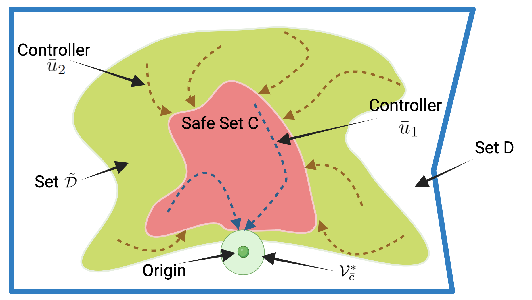
This section formalizes our control design idea to solve Problem 1. Let , , , be continuously differentiable functions, and define as in (4). Suppose that is connected and . For any , let . Next we present the main result of the paper, which solves Problem 1 and is illustrated in Figure 1.
Proposition IV.1
(Invariance and convergence to smallest compatible Lyapunov level set): Suppose that is a SBNCBF of . Let be such that and suppose that and are a compatible WCLF-SBNCBF pair in . Let be a locally Lipschitz controller such that
-
(i)
satisfies (3) for all ;
-
(ii)
for all there exists a neighborhood of such that satisfies (6) for all and .
Moreover, let be the set where the SBNCBF is feasible (cf. Definition II.2), and suppose that is connected. Let be a locally Lipschitz controller such that for all , there exists a neighborhood of such that satisfies (6) for all and . Define
and consider the closed-loop system
| (7) |
Then, (7) has a unique Filippov solution from any initial condition . Moreover, for any ,
-
(i)
if , then for all ;
-
(ii)
if , then there exists such that and for all ;
-
(iii)
if and for all , then there exists such that and for all . Moreover, there exists such that and for all .
The following result specializes Proposition IV.1 to the case where the origin is in and and are a compatible WCLF-SBNCBF pair in .
Corollary IV.2
(Invariance and convergence to the origin): Suppose that is a SBNCBF of . Further suppose that and are a compatible WCLF-SBNCBF pair in and . Let be as in Definition II.2. Take and define , and as in Proposition IV.1. Then, (7) has a unique Filippov solution from any initial condition . Moreover,
-
(i)
if , then for all and ;
-
(ii)
if and for all , then there exists such that and for all . Moreover, .
Leveraging Proposition IV.1 and Corollary IV.2, our control design methodology takes the following steps.
-
(1)
Find a WCLF and identify the set ;
-
(2)
Find a set and a SBNCBF of ;
-
(3)
Find a sublevel set of such that and are a compatible WCLF-SBNCBF pair in .
Remark IV.3
(Classical solutions): In general, the controller in Proposition IV.1 and Corollary IV.2 is discontinuous. However, if is locally Lipschitz, then the results in Proposition IV.1 and Corollary IV.2 hold with classical (instead of Filippov) solutions. Indeed, if is continuous at then the set is equal to and Filippov solutions coincide with classical ones.
Remark IV.4
(Conditions on ): Proposition IV.1 requires that for all . In general, this condition is difficult to verify. However, this condition holds if or is a superlevel set of .
Remark IV.5
(Stability of the origin): Under the assumptions in Corollary IV.2:
-
(i)
if the origin is in , Corollary IV.2 guarantees that the origin is asymptotically stable;
-
(ii)
if the origin is in , Corollary IV.2 guarantees that the origin is asymptotically stable relative to . However, in this case Lyapunov stability of the origin is not guaranteed, since trajectories that start close to but outside of it might take a long excursion away from the origin before entering and converging to it;
-
(iii)
the origin can not be outside of . Indeed, Proposition IV.1 guarantees that we can design a controller that makes all trajectories with initial condition in stay in for all future times and always decrease the value of , which is not possible if the origin is not in .
Remark IV.6
(Lipschitz controller with relaxed CLF condition): If the controller in Proposition IV.1 and Corollary IV.2 cannot be designed continuously, we give the following alternative design. Let be a locally Lipschitz controller satisfying (6) and the relaxed version of (3) , where . For example, given , one can take
| (8) | ||||
The work [16] gives conditions under which is locally Lipschitz. Even though has no stability guarantees because the CLF condition is relaxed, in Section V we show how this controller has good performance properties in practice.
Remark IV.7
(Compact safe sets): Even though Proposition IV.1 does not require to be compact, verifying its assumptions is often easier if is compact (for example, using Lemma .1). If is not compact, we can take large enough so that and consider a new compact safe set defined by . Moreover, if is a WCLF in and and are a compatible WCLF-SBNCBF pair in , then it follows that is an SBNCBF of and and are a compatible WCLF-SBNCBF pair in .
V Illustrative Examples
We demonstrate our control design in three examples.111Open-source implementations of the examples are available at https://github.com/KehanLong/CBF_Stabilization.
Example V.1
Let be defined as if and if . We note that is locally Lipschitz and consider the dynamics
| (9) |
with the state and the input. The function , , is a WCLF. Since , the set in Definition II.1 can be taken as . Now, define as and let . Note that is not compact but for any we can define a compact subset of it as , using the construction in Remark IV.7. Note that . Next, we show that for any , is a SBNCBF of and is a compatible WCLF-SBNCBF pair in .
is a SBNCBF of . Since is only defined by a single continuously differentiable function, and , for all with and , there exists a neighborhood of such that (6) is feasible for all points in for any and . At points where , and , (6) is feasible in a neighborhood of because is a WCLF. Finally, if is such that and , the fact that (6) is feasible in a neighborhood of follows from the fact that and are a compatible WCLF-SBNCBF pair, which we show next. Since the SBNCBF condition is feasible for all points in , Lemma .1 ensures that is a SBNCBF of .
and are a compatible WCLF-SBNCBF pair in . Let . If , there exists a neighborhood of and sufficiently negative and large in absolute value such that (3) and (6) are simultaneously feasible for all points in for any , extended class function and positive definite function . If and , there exists a sufficiently small neighborhood of and a positive definite function with sufficiently small such that any that satisfies (6) for , also satisfies (3) at . Hence, there exists sufficiently small such that and are a compatible WCLF-SBNCBF pair for all with . Finally, take , with , , let , and take with . It follows that , which implies that and are a compatible WCLF-SBNCBF pair at (cf. [10, Lemma 5.2]). Hence, we have proved that and are a compatible WCLF-SBNCBF pair in . Now, the fact that and are a compatible WCLF-SBNCBF pair in all of follows from the fact that is a WCLF and by constructing a linear extended class function with a similar argument as in Lemma .1. Now, by using Lemma .1 it follows that for any , is a SBNCBF of and the set in Definition II.2 can be taken as . Moreover, and are a WCLF-SBNCBF compatible pair in . Therefore, the results in Corollary IV.2 apply.
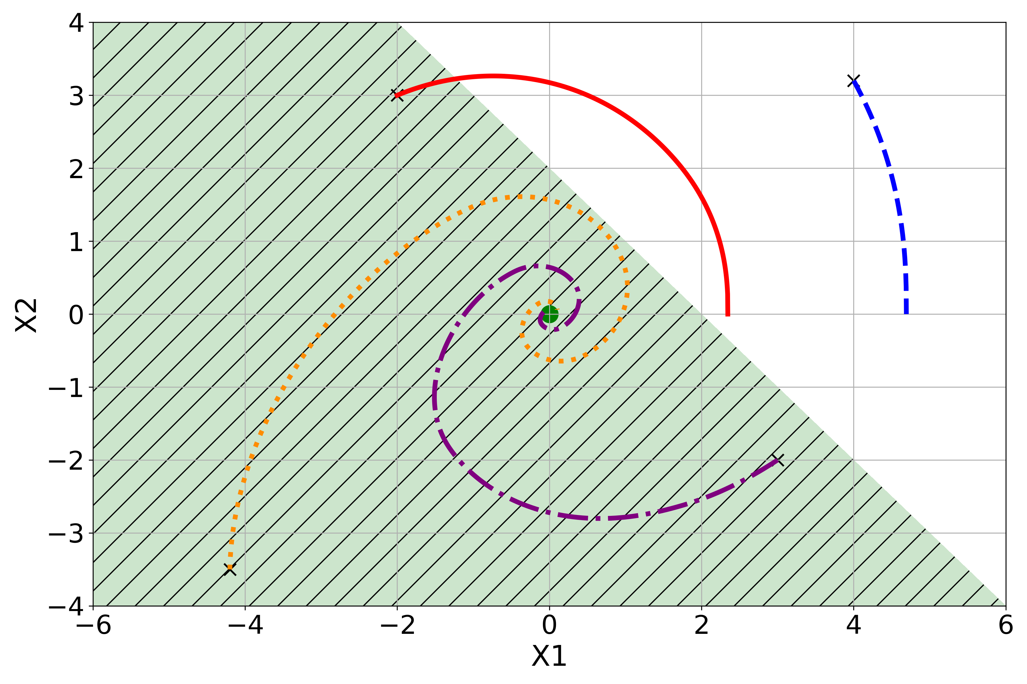
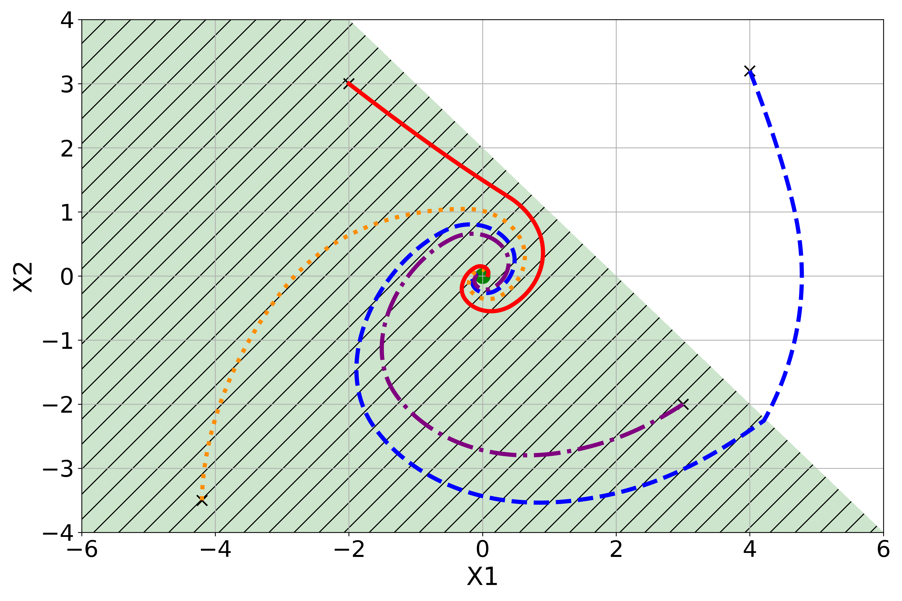
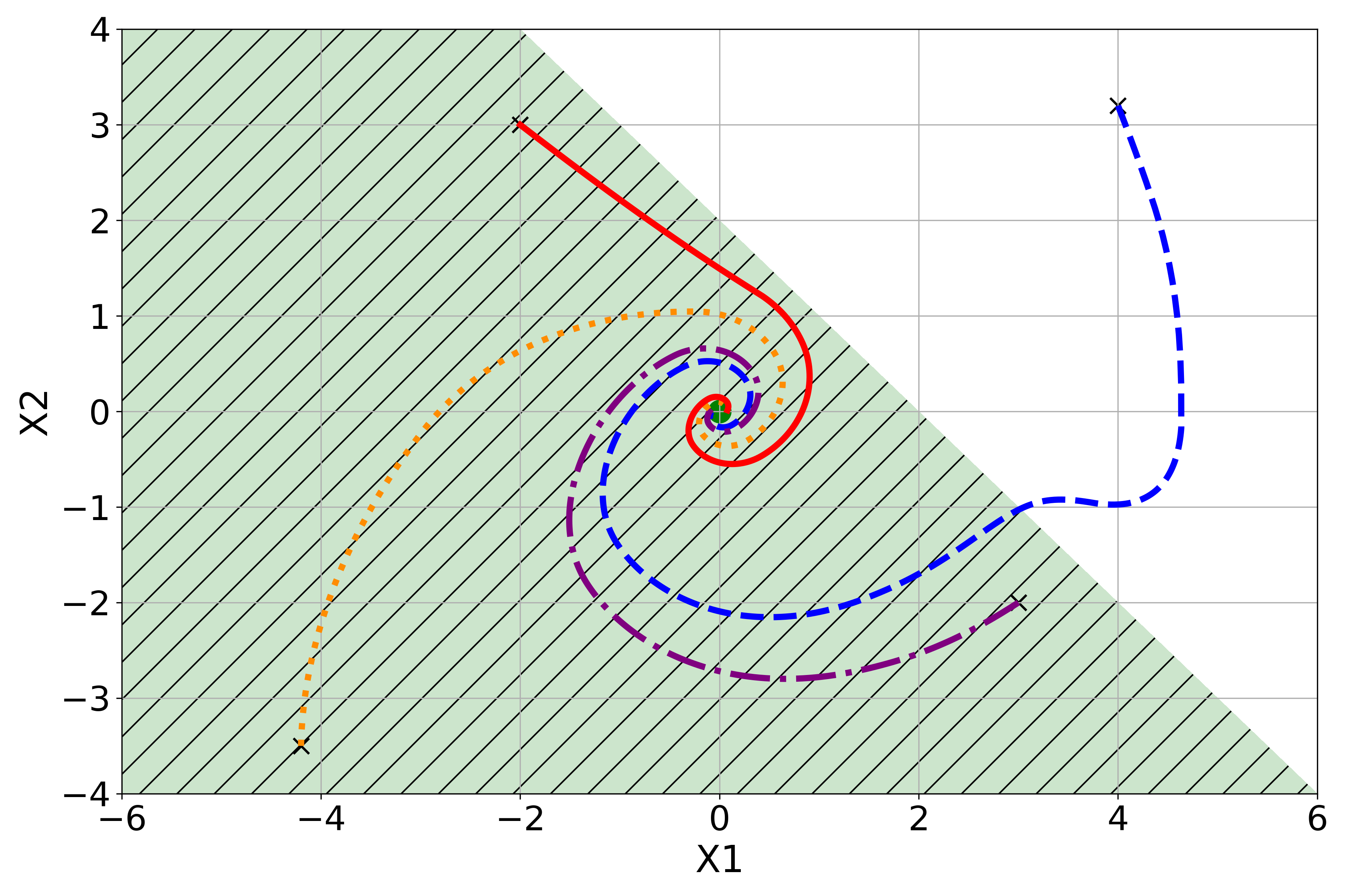
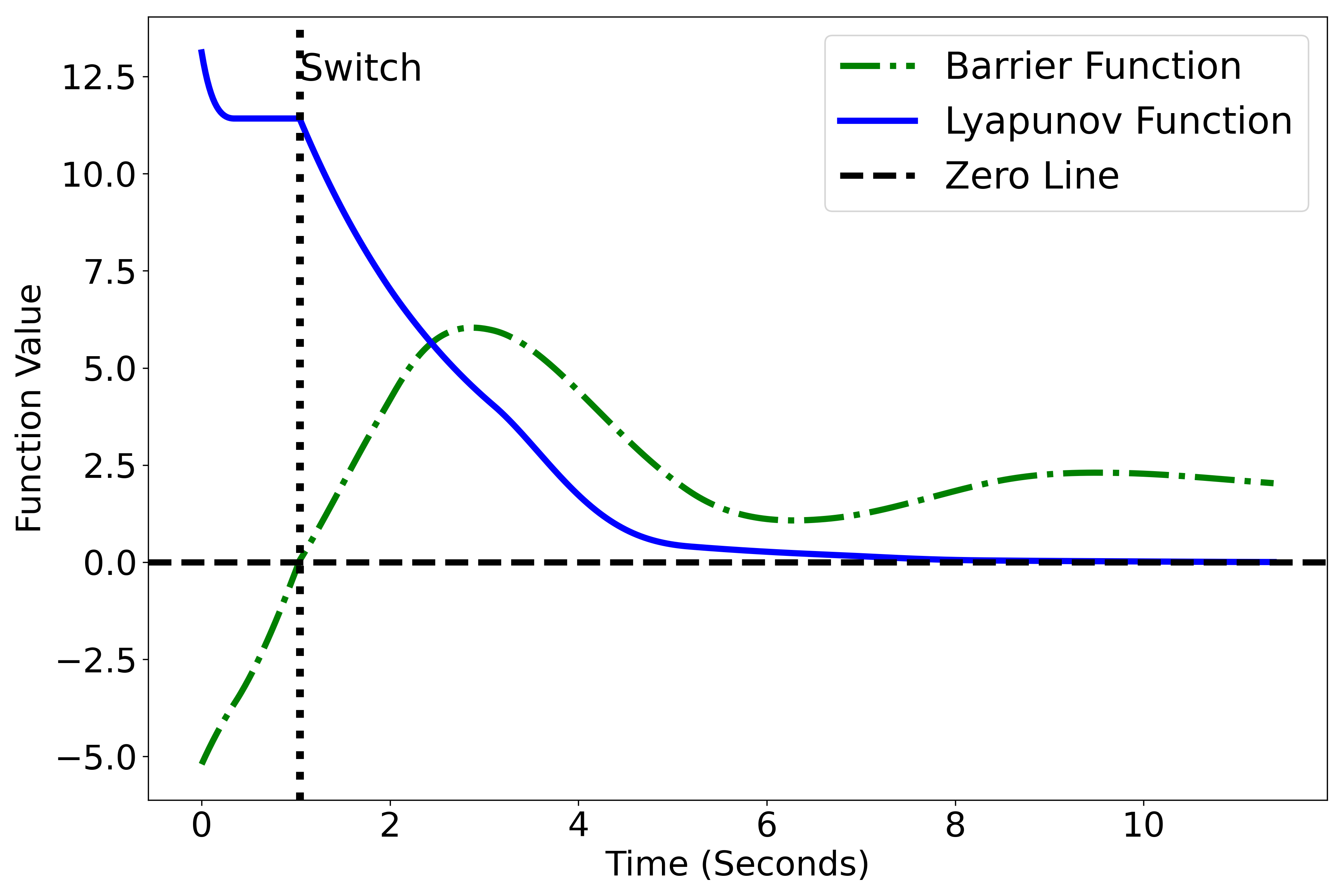
Simulation results. In the simulation, we set as and as for all . In Fig. 2, we compare the performance of the controller obtained as the solution of the quadratic program (QP) that at every state minimizes the norm of the controller and satisfies only (3) (denoted as WCLF-QP), the controller obtained as the solution of the QP that at every state minimizes the norm of the controller and satisfies (3) and (6) for all and satisfies the assumptions of Proposition IV.1 (denoted as switching WCLF-SBNCBF-QP) and the relaxed WCLF-SBNCBF-QP controller (presented in Remark IV.6) for four initial states. In Fig. 2(a), the WCLF-QP fails to stabilize the system for two initial states, since (3) cannot be satisfied once and . On the other hand, both the switching WCLF-SBNCBF-QP and the relaxed WCLF-SBNCBF-QP controller successfully stabilize the system. Moreover, when the system is outside the safe set, the satisfaction of the SBNCBF condition drives the system to the safe set, leading to a temporary non-decrease in Lyapunov function values. At around seconds, the system enters the safe set, and the satisfaction of the WCLF and SBNCBF conditions ensures stabilization to the origin without leaving the safe set.
Example V.2
Consider unicycle dynamics:
with state and inputs . We consider stabilizing the system at the origin but our approach can be adapted to stabilize the system at any point in 3. Consider the WCLF , with a parameter to be designed. Let be the associated positive definite function in Definition II.1. Note that is not a CLF and the CLF condition (3) reads
| (10) |
If and , then (10) cannot be satisfied unless . Therefore, the set in Definition II.1 can be taken as
Now, let and define
| (11) |
Further, let , which is connected, but not compact. Let be a compact subset of obtained using the compactification procedure described in Remark IV.7 and followed in the previous example. Following an argument similar to the previous example, it is sufficient to show that satisfies the SBNCBF condition at and that and are a compatible WCLF-SBNCBF pair in , where is a small sublevel set of to be designed. We first show that the set (and hence also ) is a subset of , as required in Definition II.1. Throughout this example we let . and .
The set inclusion holds. Suppose that and . Then, and . Since and are orthogonal and and are also orthogonal, is proportional to . By the Cauchy-Schwartz inequality, this means that . Now, if , . This means that and thus , reaching a contradiction.
is a SBNCBF of . We show that there exists and an extended class function such that for all , there exists a neighborhood such that (6) is feasible. First, suppose that and . Condition (6) at for reads
| (12) |
Note that . Moreover, . Indeed, if , then by the same argument used to show that we have , where in the last inequality we have used . This contradicts . Hence, and, if and , there exists a neighborhood of for which (12) is feasible at all points in for any and . Next, suppose and . Condition (6) at for reads
| (13) |
If , by the same argument used to show , we have that , which contradicts . Hence, there exists a neighborhood of for which (13) is feasible for all points in for any and . Lastly, if , since (12) can be satisfied using only and (13) can be satisfied using only , there also exists a neighborhood of for which (12) and (13) are simultaneously feasible for all points in for any and .
Compatible region for and . Let and such that for all (which exists because is compact), and take . Using the notation in Section IV, we show that and are a compatible WCLF-SBNCBF pair in . First, we show that and are compatible in . We use [10, Lemma 5.1], which gives a characterization of when a CLF and a CBF are compatible at a point. Let and suppose that there exists such that
| (14) |
Then, , which implies that the WCLF condition for only involves and the SBNCBF condition for only involves . Therefore, inequalities (3) for and (6) for can be satisfied simultaneously in a neighborhood of for any and . This implies that and are a compatible WCLF-SBNCBF pair in . Now, let be a continuous controller satisfying the WCLF condition for and the SBNCBF condition for for all . Such controller exists by [17, Proposition 3.1], by taking sufficiently small. Since and , for all . Now, consider the linear extended class function , with
| (15) |
the right hand side of (15) is bounded because is continuous and is compact. Using as extended class function, satisfies the WCLF condition for and the SBNCBF condition for . Hence, and are a compatible WCLF-SBNCBF pair in . Hence, the assumptions of Proposition IV.1 hold and our control design ensures that all trajectories that start in converge to . The fact that satisfies the SBNCBF condition at ensures that there exists a set containing as in Definition II.2. However, (6) is in general not feasible outside of .
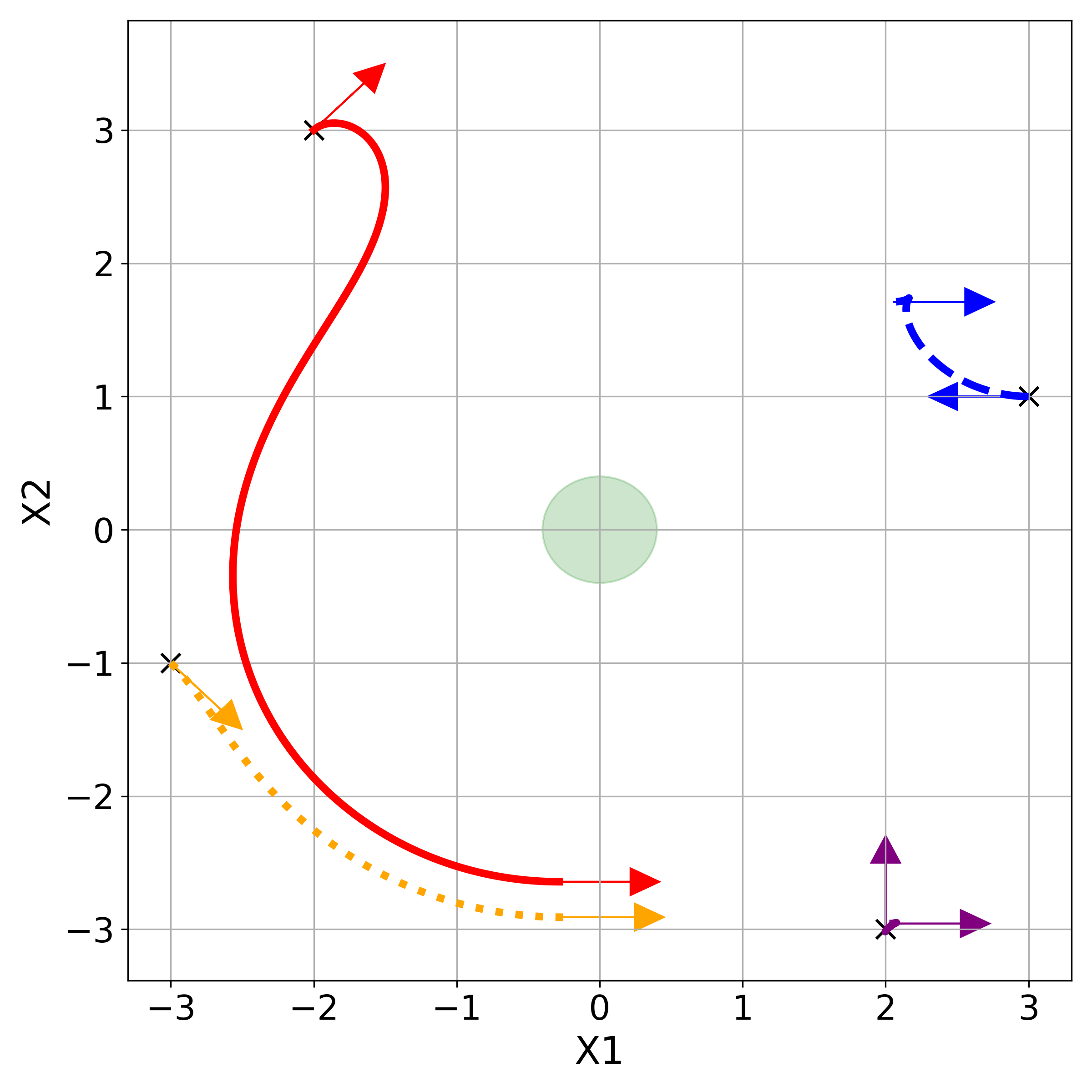
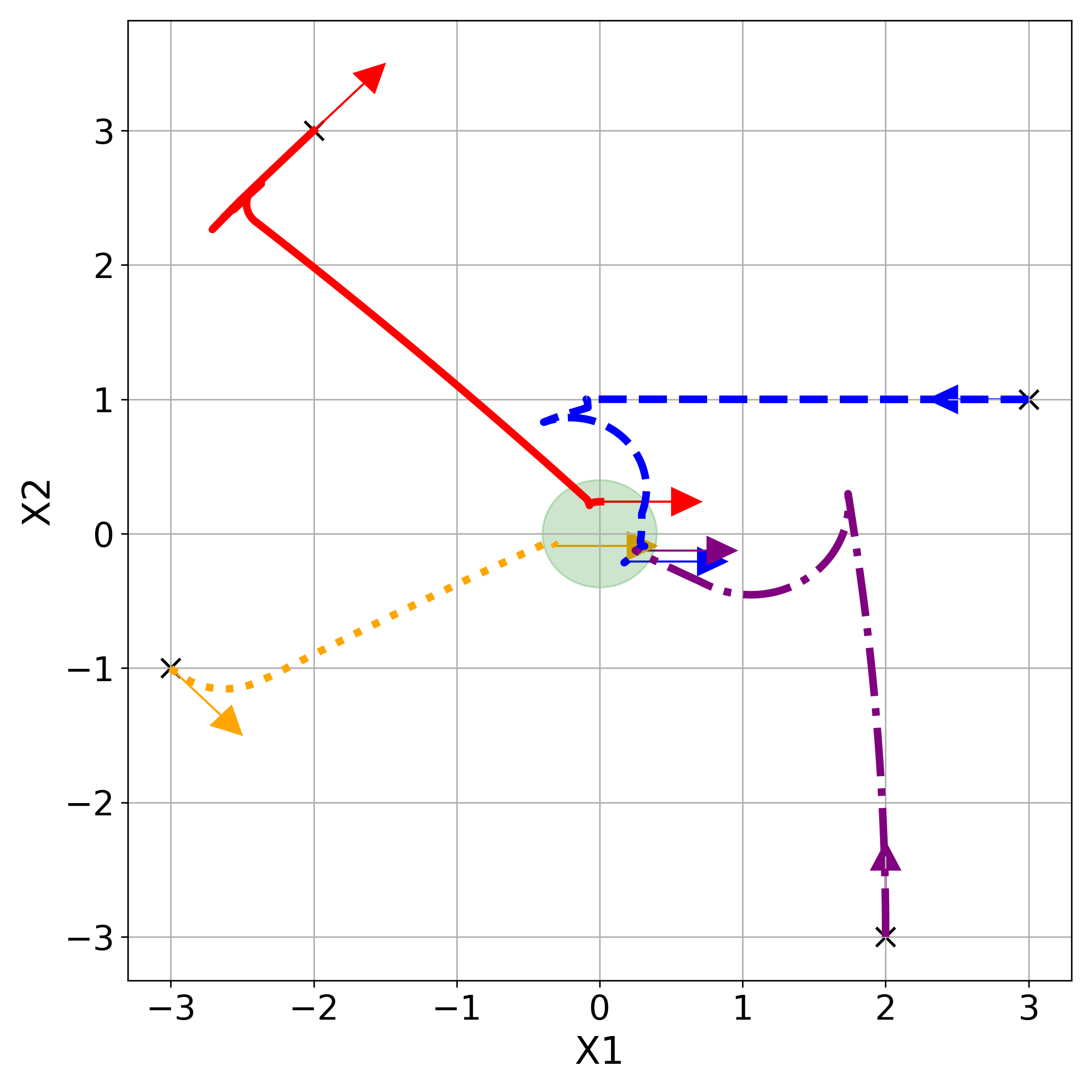
Simulation results. In the simulation, we specify , , positive-definite function , and define the extended class function . As shown in Fig. 4(a), relying solely on the WCLF fails to stabilize the system to the origin, since trajectories end up at points where the CLF condition is not feasible. However, as shown in Fig. 4(b), the switching WCLF-SBNCBF QP controller converges to a neighborhood of the origin .
VI Conclusions
This paper proposed an approach for stabilizing nonlinear systems using weak CLFs that are not valid CLFs. Our key idea is to treat the subset where the CLF condition is feasible as a safe set and utilize a non-smooth CBF to keep the system trajectories in the safe set. We proved that the proposed controller has stability guarantees both when it is continuous or discontinuous, using appropriate notions of solution for the closed-loop system. Our methodology requires the identification of a WCLF-SBNCBF pair, together with a set where both are compatible. We have illustrated this process in different examples. Future work will focus on three fronts. Firstly, we aim to develop theoretical and computational tools to simplify the process of identifying a compatible WCLF-SBNCBF pair. Secondly, we plan to investigate explicit control designs that satisfy the requirements in our results and ensure continuity of the resulting controller. Thirdly, we plan to extend our method to systems with uncertainty.
Acknowledgements
The authors are grateful to M. Alyaseen for multiple conversations on barrier functions for discontinuous systems.
References
- [1] E. D. Sontag, Mathematical Control Theory: Deterministic Finite Dimensional Systems, 2nd ed., ser. TAM. Springer, 1998, vol. 6.
- [2] W. Tan, “Nonlinear control analysis and synthesis using sum-of-squares programming,” Ph.D. dissertation, University of California, Berkeley, 2006.
- [3] Y.-C. Chang, N. Roohi, and S. Gao, “Neural Lyapunov control,” in Conference on Neural Information Processing Systems, vol. 32, Vancouver, Canada, Dec. 2019, pp. 3240–3249.
- [4] P. Wieland and F. Allgöwer, “Constructive safety using control barrier functions,” IFAC Proceedings Volumes, vol. 40, no. 12, pp. 462–467, 2007.
- [5] A. D. Ames, S. Coogan, M. Egerstedt, G. Notomista, K. Sreenath, and P. Tabuada, “Control barrier functions: theory and applications,” in European Control Conference, Naples, Italy, 2019, pp. 3420–3431.
- [6] P. Glotfelter, J. Cortés, and M. Egerstedt, “Nonsmooth barrier functions with applications to multi-robot systems,” IEEE Control Systems Letters, vol. 1, no. 2, pp. 310–315, 2017.
- [7] P. Glotfelter, I. Buckley, and M. Egerstedt, “Hybrid nonsmooth barrier functions with applications to provably safe and composable collision avoidance for robotic systems,” IEEE Robotics and Automation Letters, vol. 4, no. 2, pp. 1303–1310, 2019.
- [8] M. Z. Romdlony and B. Jayawardhana, “Stabilization with guaranteed safety using control Lyapunov-barrier function,” Automatica, vol. 66, pp. 39–47, 2016.
- [9] K. Long, C. Qian, J. Cortés, and N. Atanasov, “Learning barrier functions with memory for robust safe navigation,” IEEE Robotics and Automation Letters, vol. 6, no. 3, pp. 4931–4938, 2021.
- [10] P. Mestres and J. Cortés, “Optimization-based safe stabilizing feedback with guaranteed region of attraction,” IEEE Control Systems Letters, vol. 7, pp. 367–372, 2023.
- [11] Y. Chen, M. Jankovic, M. Santillo, and A. D. Ames, “Backup control barrier functions: Formulation and comparative study,” in 2021 60th IEEE Conference on Decision and Control (CDC), 2021, pp. 6835–6841.
- [12] A. R. Teel and N. Kapoor, “Uniting local and global controllers,” in European Control Conference, 1997, pp. 3868–3873.
- [13] A. F. Filippov, Differential Equations with Discontinuous Righthand Sides, ser. Mathematics and Its Applications. Kluwer Academic Publishers, 1988, vol. 18.
- [14] R. A. Freeman and P. V. Kototovic, Robust Nonlinear Control Design: State-space and Lyapunov Techniques. Cambridge, MA, USA: Birkhauser Boston Inc., 1996.
- [15] P. Glotfelter, J. Cortés, and M. Egerstedt, “Boolean composability of constraints and control synthesis for multi-robot systems via nonsmooth control barrier functions,” in IEEE Conf. on Control Technology and Applications, Copenhagen, Denmark, Aug. 2018, pp. 897–902.
- [16] P. Mestres, A. Allibhoy, and J. Cortés, “Regularity properties of optimization-based controllers,” European Journal of Control, 2024, available at https://arxiv.org/abs/2311.13167.
- [17] P. Ong and J. Cortés, “Universal formula for smooth safe stabilization,” in IEEE Conf. on Decision and Control, Nice, France, Dec. 2019, pp. 2373–2378.
Lemma .1
(Checking SBNCBF or compatibility conditions on the boundary is sufficient): Suppose that is a compact set.
-
(i)
Suppose that there exists and a neighborhood for all , such that for all there exists and satisfying
(16) for all . Then, is a SBNCBF of .
- (ii)