An Implicit Function Method for Computing the Stability Boundaries of Hill’s Equation
Abstract
Hill’s equation is a common model of a time-periodic system that can undergo parametric resonance for certain choices of system parameters. For most kinds of parametric forcing, stable regions in its two-dimensional parameter space need to be identified numerically, typically by applying a matrix trace criterion. By integrating ODEs derived from the stability criterion, we present an alternative, more accurate and computationally efficient numerical method for determining the stability boundaries of Hill’s equation in parameter space. This method works similarly to determine stability boundaries for the closely related problem of vibrational stabilization of the linearized Katpiza pendulum. Additionally, we derive a stability criterion for the damped Hill’s equation in terms of a matrix trace criterion on an equivalent undamped system. In doing so we generalize the method of this paper to compute stability boundaries for parametric resonance in the presence of damping.
keywords:
Parametric Resonance, Stability, Hill Equation70J40, 37C75
1 Introduction
Second order oscillators with time-periodically varying system parameters can experience the related phenomena of parametric resonance and vibrational stabilization. Parametric resonance involves exponential amplitude growth under certain combinations of the oscillator’s ostensible “natural frequency” and parametric forcing amplitude. Parametric forcing refers to the effect of a time-periodic system parameter that (typically) multiplies the state, and differs from the more typical additive harmonic forcing in this way. Parametric resonance in observed in a variety of natural and engineered systems, such as in hydrodynamic instabilities [7, 1], time-periodic axial loading of columns [6] and in MEMS devices subjected to alternating voltage [3].
A canonical model for linear second order systems that can undergo parametric resonance is Hill’s equation [10], a harmonic oscillator with a time-periodically varying spring constant. Certain combinations of the system’s natural frequency and parametric forcing amplitude can cause instability, even at arbitrarily low forcing amplitudes under low or zero damping conditions. These unstable parameter ranges form the well-known Arnold tongue structures [12].
Vibrational stabilization, the flip side of parametric resonance, involves the stabilization via time-periodic parametric forcing of nominally unstable systems, typically a second order oscillator with a negative spring constant. A common example of this is the Kapitza pendulum, an inverted pendulum stabilized via sinusoidal base motion that acts as sensorless feedback. Although previously considered a high-frequency phenomenon, recent work by Berg [2] shows that vibrational stabilization can be achieved via parametric forcing at lower frequencies with precisely chosen amplitudes.
The stability boundaries in parameter space of both Hill’s equation and the linearized Kapitza pendulum are determined by specific contours of an implicit function of the system parameters. This provides a two-dimensional stability map for both kinds of systems. Such maps have been used in the design of quadrupole ion traps for mass spectrometry [8]. While canonical models of both phenomena are typically of second order, higher order systems can be modeled as collections of Hill oscillators [4] or their unstable counterparts [5] under certain conditions, and stability criteria can be found as the composition or overlap of the individual two-dimensional stability maps of the component systems.
It is possible to derive analytical criteria for parametric resonance in the limit of small parametric forcing [12] using the classical Floquet theory [2], and for vibrational stabilization using higher-order averaging methods [9]. However, these results are valid in limited regimes – respectively, in the limit of low parametric forcing amplitudes and frequencies for parametric resonance and vibrational stabilization. More general estimates require numerical computation. Typically these boundaries are computed and visualized via contour plots of the system, as computed using a marching squares algorithm [11]. In this work we propose a more efficient method involving direct numerical calculation and integration of this implicit function. This method leans on the idea that we are only interested in specific contours and not the overall picture, reducing the numerical complexity of the problem.
To illustrate the method, we cover the general idea of integrating an implicit function of two variables in Section 2. For Hill’s equation this function does not have a closed form, so we cover some relevant properties in Section 3.1, additional solution steps required in Section 3.2, and provide some examples of the results of this method. Section 3.3 extends the numerical method to the case of Hill’s equation with damping. Finally, we cover some considerations for numerical integration in Section 4.
2 The Implicit Function Method for Contour Plots
The general idea of the method is as follows: given a smooth function of variables , , we wish to plot a specific contour in space passing through , where .
The condition is an implicit definition of the curve or that we seek, and we can find differential equations for them:
| (4) |
Where at least one of the two equations is well-defined in a neighborhood of . We note that neither the ODEs nor the initial conditions involve – these ODEs are satisfied by the contour of that passes through irrespective of its value.
Without loss of generality, we assume in some neighborhood of , so that that the curve is locally well defined. Then we may write
| (5) |
Since is known, this ODE can be readily solved to the required precision. During numerical computation, the case of can be identified by large changes in (if using fixed time steps), by stiffness checks or progressively smaller time steps (if using adaptive time stepping), and the reciprocal problem can be solved instead.
3 Application to Hill’s Equation
We apply this method to finding the stability boundaries in parameter space for Hill’s equation
| (6) | |||
which represents a harmonic oscillator with a periodically varying spring constant. is the mean value of the spring constant, and is the parametric forcing amplitude. The parametric forcing has zero mean. Such systems can experience parametric resonance for specific choices of and . Allowing to be negative gives us the linearized model of the Kapitza pendulum, an inverted pendulum with sinusoidal vertical base motion. This nominally unstable system is vibrationally stabilized for specific choices of and . Our treatment of stability boundaries covers both regimes of behavior.
3.1 Properties of Hill’s Equation
We review a few salient properties of Hill’s equation for applying the implicit function method to compute its parametric stability.
In first order form, Eq. 6 has a Hamiltonian generator and thus a symplectic state-transition matrix (henceforth just and ):
| (7) | ||||
| (8) |
The stability of this linear, time periodic system depends on the spectral radius of its “monodromy map”, its state transition matrix evaluated at one forcing period . The system is stable if its spectral radius is or smaller, and unstable if it is larger.
This stability condition can be simplified as follows: has determinant for all , as it is symplectic. This can be verified directly as:
Since , it is for all time.
Together, the conditions , and the fact That is real and imply that system (6) is stable iff .
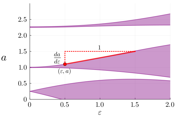
The condition is a function of two variables whose contours in space with values form the boundary between regions of stability and regions of parametric resonance. These boundaries in parameter space form the well known Arnold tongue structures associated with parametric resonance (Fig. 1).
For Hill’s equation, the theory of linear time-periodic systems provides many analytical methods to find the positions of the tongues in the limit . Perturbation analysis, the method of Hill’s determinants [14] and Floquet multipliers [12] are three common methods. The primary result is the following: In the limit , system (6) is unstable when is a half-multiple of the forcing frequency , i.e. when
| (9) |
Further, it can be shown [12] that there are no other values of (with ) for which the system is unstable.
3.2 Stability Boundary Computation for Hill’s Equation
The stability boundaries are typically computed in the following way:
-
1.
Create a grid in space that covers the parameter ranges of interest.
-
2.
Find the monodromy map (and thus its trace) numerically at all points on this grid.
-
3.
Plot the contours of the map that have values .
This method has three shortcomings. The first is the computational burden of calculating the value of at all grid points. Essentially, this involves scanning a two dimensional space in search of a one-dimensional curve. The second is that the slope of the curve is not known apriori, so the spatial grid resolution cannot be adjusted to take advantage of this. As a result, several runs with progressively finer grids are required to obtain a suitably detailed picture. Finally, there are regions in the parameter space where changes rapidly with , making it difficult to resolve fine details in these areas in a contour map created with a typical Marching Squares algorithm.
Applying the implicit function method outlined in Section 2 avoids all of these shortcomings, but it requires knowledge of at least one point on the contour of interest. Specifically, for each contour such that , we need to know the corresponding . From Eq. 9, this point is .
We can now apply the above method to find the stability boundaries for Hill’s equation. To find such that
we formulate the equivalent of Eq. 5 for this problem:
| (10) |
The slope of a stability map boundary in space is illustrated in Fig. 1. To calculate and , we can use Hill’s equation (7). Differentiating the original system with respect to the parameters and :
| (11) | ||||
| (12) | ||||
| (13) |
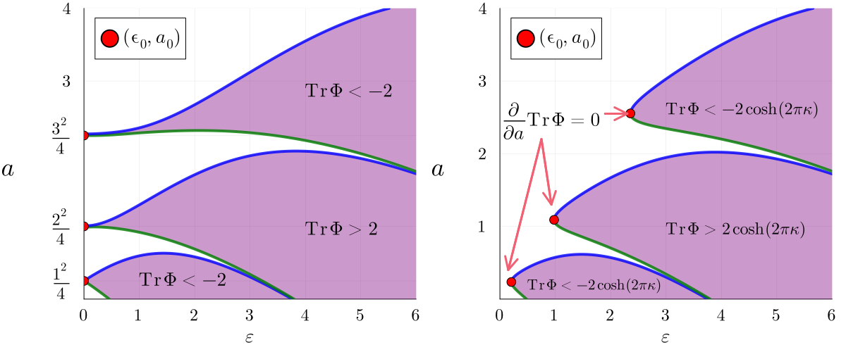
Where we have suppressed the explicit dependence of and on and in the notation. The linear ODEs (12) and (13) can be integrated from to to give and respectively. Since uniformly for any choice of and , the initial conditions are uniformly zero in the above equations, and they are driven by the state transition matrix at , which appears as an additive input. This recipe for finding stability boundaries is illustrated in Fig. 2 and Fig. 5.
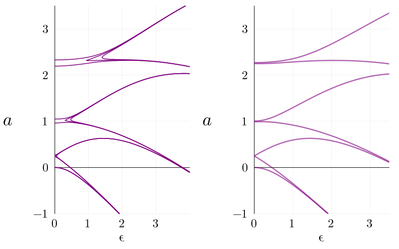
Fig. 3 compares the stability maps for Hill’s equation as computed using the contour method and the implicit function method introduced in this paper. The implicit function method provides better resolution with significantly less computational effort.
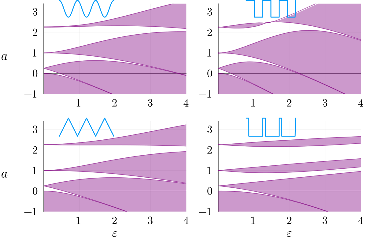
Fig. 4 shows the stability boundaries computed using this method for Hill’s equation with a few different parametric forcing functions.
3.3 Stability boundaries for Hill’s equation with damping
In this section we apply the implicit function method of Section 3.2 to Hill’s equation with viscous damping coefficient :
| (14) |
Through the transformation , it is possible to derive an equivalent stability criterion for a related (undamped) Hill equation.
Theorem 3.1.
Proof 3.2.
See Appendix A.
Since , the Arnold tongues for Hill’s equation with damping do not meet on the axis, and there is no equivalent to criterion (9). Integrating Eq. 10 along the contour thus requires finding one point along each “branch” of the stability boundary.
We find these initial conditions numerically, using the criteria and . The rest of the treatment is identical to the undamped case covered in Section 3.3. Fig. 5 illustrates the method.
4 Considerations for Numerical Integration
In this section we briefly mention some details of and considerations for the numerical integration of Eq. 10.
-
•
Since the Hill equation is a Hamiltonian dynamical system, Eq. 11 needs to be solved using a symplectic integrator. Depending on the required accuracy, a symplectic Euler method or an “almost symplectic” trapezoidal method can suffice.
- •
-
•
Since where two Arnold tongues meet, the integration for Eq. 10 can stall around these points. We switch conditionally to solving the reciprocal problem when appropriate:
- •
5 Extensions and Limitations of the Implicit Function method
The implicit function method detailed in Section 2 can be applied to compute specific contours of any smooth scalar-valued function more efficiently than evaluating the function on a grid.
While the method provides better resolution of the tongues compared to plotting contours of the trace of the monodromy map, it also rests on certain assumptions about the geometry of the Arnold tongues, for instance that the stability boundaries are smooth and representable in the form . It is thus not a true parametric description of the stability boundaries of the form for some parameter , and requires careful handling of “crossover” points of the Arnold tongues, where two tongues meet.
It is also reliant on the existence of a scalar criterion for stability, of the form . The stability criterion for parametric resonance in higher-order linear systems involves the eigenvalues of the monodromy map that is not reducible to a criterion involving its trace. When the system cannot be diagonalized into a collection of decoupled second order time-periodic oscillators, neither the contour method nor the implicit function method discussed in this paper can be directly applied to obtain stability maps. Extending the method to generate the stability maps of higher order systems, possibly using the symplectic properties of the monodromy map, is a promising avenue of future work.
References
- [1] Benjamin and Ursell, The stability of the plane free surface of a liquid in vertical periodic motion, Proceedings of the Royal Society of London. Series A. Mathematical and Physical Sciences, 225 (1954), pp. 505–515, https://doi.org/10.1098/rspa.1954.0218.
- [2] J. M. Berg and I. M. Wickramasinghe, Vibrational control without averaging, Automatica, 58 (2015), pp. 72–81, https://doi.org/10.1016/j.automatica.2015.04.028.
- [3] D. I. Caruntu and I. Martinez, Reduced order model of parametric resonance of electrostatically actuated MEMS cantilever resonators, International Journal of Non-Linear Mechanics, 66 (2014), pp. 28–32, https://doi.org/10.1016/j.ijnonlinmec.2014.02.007.
- [4] K. Chikmagalur and B. Bamieh, Parametric Resonance in Networked Oscillators, June 2024, https://doi.org/10.48550/arXiv.2406.11117, https://arxiv.org/abs/2406.11117.
- [5] K. Chikmagalur and B. Bamieh, Vibrational stabilization of multi-link mechanical systems, Automatica, 165 (2024), p. 111589, https://doi.org/10.1016/j.automatica.2024.111589.
- [6] T. Iwatsubo, Y. Sugiyama, and S. Ogino, Simple and combination resonances of columns under periodic axial loads, Journal of Sound Vibration, 33 (1974), pp. 211–221.
- [7] R. E. Kelly, The stability of an unsteady Kelvin–Helmholtz flow, Journal of Fluid Mechanics, 22 (1965), pp. 547–560, https://doi.org/10.1017/S0022112065000964.
- [8] W.-W. Lee, S.-K. Min, C.-H. Oh, P.-S. Kim, S.-H. Song, M. Yang, and K. Song, Stability of ion motion in the quadrupole ion trap driven by rectangular waveform voltages, International Journal of Mass Spectrometry, 230 (2003), pp. 65–70, https://doi.org/10.1016/j.ijms.2003.08.008.
- [9] M. Maggia, S. A. Eisa, and H. E. Taha, On higher-order averaging of time-periodic systems: Reconciliation of two averaging techniques, 99 (2019), pp. 813–836, https://doi.org/10.1007/s11071-019-05085-4.
- [10] W. Magnus and S. Winkler, Hill’s Equation, Courier Corporation, Jan. 2004.
- [11] C. Maple, Geometric design and space planning using the marching squares and marching cube algorithms, in 2003 International Conference on Geometric Modeling and Graphics, 2003. Proceedings, July 2003, pp. 90–95, https://doi.org/10.1109/GMAG.2003.1219671.
- [12] A. H. Nayfeh and D. T. Mook, Nonlinear Oscillations, Wiley, May 1995, https://doi.org/10.1002/9783527617586.
- [13] B. Owren and M. Zennaro, Derivation of Efficient, Continuous, Explicit Runge–Kutta Methods, SIAM Journal on Scientific and Statistical Computing, 13 (1992), pp. 1488–1501, https://doi.org/10.1137/0913084.
- [14] N. M. Wereley, Analysis and Control of Linear Periodically Time Varying Systems, PhD thesis, Massachusetts Institute of Technology, 1990.
Appendix A Hill’s equation with damping
In this section we review properties of the monodromy map of the damped Hill’s equation that we use in Section 3.3.
Hill’s equation with damping is (see Eq. 14)
| (16) |
The state-transition matrix for this system is given, as before, by , henceforth just . This can be transformed into the undamped Hill equation through the variable substitution :
| (17) | ||||
| (18) |
where we have defined the transformation matrix
| (19) |
The nominal spring constant in the transformed coordinates is lower than the original by . We denote the state transition matrix for system (18) as , suppressing the dependence on the parameters , and .
System (14) is unstable when has an eigenvalue outside the unit circle. Our goal is to obtain an equivalent stability criterion for the damped system Eq. 14 in terms of the monodromy map of the transformed system. The implicit function method of Section 3 can then be applied to the transformed, undamped system to plot the stability map of the original damped system. To do this we use the following property of the solution of the damped Hill’s equation:
Lemma A.1.
The monodromy map of the damped Hill equation (14) is a scalar multiple of a symplectic matrix. Specifically, is symplectic.
Proof A.2.
From Eq. 17, we can express the monodromy map in terms of that of the original damped system:
so that . We note that is and , so it is symplectic as well. Thus
| (20) |
is a product of three symplectic matrices and is also symplectic.
When has an eigenvalue at , has an eigenvalue at . Since the latter matrix has determinant , its other eigenvalue is at . Next, we observe that and are related by a similarity transform Eq. 19, so their eigenvalues and matrix traces are the same. The instability criterion for in terms of the transformed Eq. 18 is thus
| (21) |
This result is summarized in Table 1. We note that , with the lower bound achieved in the undamped case of .
| Hill’s equation: | Damped | Transformed (undamped) |
|---|---|---|
| System | ||
| State | ||
| Monodromy map | ||
| Stability criterion |