Quadrupole-Octupole Residual Interaction
in the Proxy- Scheme
Abstract
The octupole deformation of atomic nuclei is a relevant research area given its implications in the nuclear structure and fundamental physics, however, inclusion of octupole degrees of freedom in the nuclear interaction has been explored little in symmetry-based models. In this article we expand the octupole operator in the second quantization formalism and use it to formulate an octupole-octupole residual interaction which is incorporated in Elliott’s model Hamiltonian. We compute the matrix elements of this extended Hamiltonian and use them to calculate energy levels and analyse the transition strength of the isotope 224Th using the semi-microscopic algebraic quartet model (SAQM) based on the proxy- scheme.
I INTRODUCTION
The atomic nucleus is a primary component of ordinary matter and its structure is one of the main subjects of study in quantum mechanics. Since the nucleus is an extended body, it is a legitimate area of research to investigate its geometrical shape [1, 2, 3], the interactions influencing it [4] and its variation across isotopes as well as between excited states [5, 6]. It is known that some nuclei organize in spherical shapes while others lower its energy through deformation. This phenomenon is described theoretically using the multipole moments where the most relevant for the atomic nucleus are the first four, viz. dipole (), quadrupole (), octupole () and hexadecapole () moments.
Over the years, several non-zero values of electric quadrupole moments have been reported [7] which indicate axially symmetric ellipsoidal deformations of the nucleus. Negative values correspond to oblate deformations while positive ones to prolate deformations, with a clear prolate dominance observed across all nuclei [8, 4]. The largest quadrupole values are generally found in half-filled shells defined by the magic numbers and . This breaking of spherical symmetry allows for rotational degrees of freedom to populate excited states observed as characteristic energy level patterns called rotational bands.
For certain configurations of proton () and neutron () numbers around , and [9], the nucleus lowers its energy further through a static octupole deformation [10, 11]. This combined with a prolate quadrupole moment gives the nucleus a so-called “pear shape”[12, 13]. Such mirror asymmetric shape causes a displacement between the centers of charge and mass, creating an electric dipole moment as well. Although few direct measurements of the moments have been reported in the literature, certain low energy spectra, enhanced and transition probabilities serve as indirect indicators of octupole deformation [9].
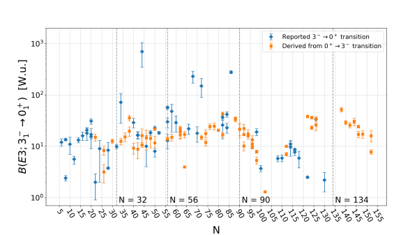
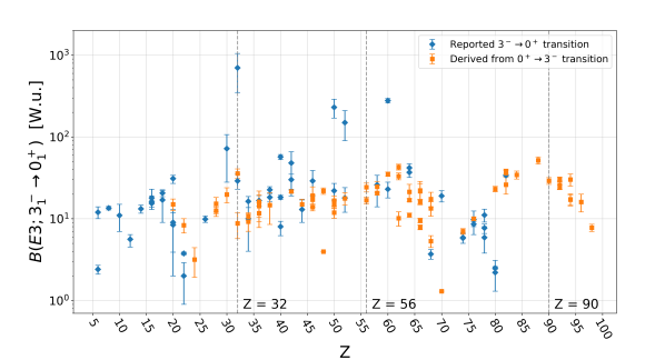
In particular, for even-even nuclei, the presence of a negative parity band near the ground state band is a characteristic spectrum of “pear shape” deformation along with enhanced and transitions. In figure 1 are shown the energies of the lowest and excited states for even-even nuclei. It can be observed that the lowest values are found in the actinide region for the isotopes 224Ra, 224Th, 226Th, 222Ra, 226Ra and 228Th in increasing order up to 0.4MeV. In figure 2 are shown the evaluated values where a maximum can be found around that region. Previous calculations [14] with relativistic Hartree–Bogoliubov (RHB) theory predicted stable octupole deformations for isotopes 222-226Ra and 224-228Th suggesting them as the best even-even candidates for research on “pear shape” deformation.
One of the main interests of studying octupole collectivity in nuclei goes further than the nuclear structure itself, having implications in the strong nuclear interaction and the symmetries of nature [15, 16]. Experimental efforts are being made to measure , and transitions that will provide more insight about fundamental physics [17, 18]. In this article we continue the work on the isotope 224Th in the semi-microscopic algebraic quartet model (SAQM) [19] based on the proxy- scheme [20, 21] started in [22, 23] by including a residual octupole-octupole interaction in Elliott’s Hamiltonian. An analysis of octupole effective charges and transition are made as well. We begin explaining the two-shell model space of the system required for the residual octupole interaction to be defined, then show the expansion of the octupole operator in terms of irreducible tensors and the calculations for the low-energy spectrum of 224Th along comparison with observed energy levels.


II MODEL SPACE
Since the octupole operator has negative parity, at least two consecutive shells are required for its minimal realization [26]. We will focus on heavy even-even nuclei in the actinide region so that proton () and neutron () degrees of freedom must be distinguished. These two statements imply that the full model space has to be composed of two-shells which represent the valence and excited shells states for each proton and neutron spaces ( and respectively) along with their couplings to total irreducible representations (irreps).
The spectrum generating algebra (SGA) [27] will be for each proton and neutron spaces where , the sub-indexes and indicate lower and upper shells respectively and . Since nucleons are fermions, their SGA irreps must be totally anti-symmetric given by where represents the number of particles. This algebra can be separated into spin and spatial parts as a product . The corresponding spatial representations will be denoted as . In the SAQM, the ground state () will be given by setting the upper shell empty in a configuration like where denotes the number of quartets [19, 22]. Excited () states will be given by occupying one orbital in the excited shell in the proton or neutron space (not simultaneously) denoted as . These irreps guarantee that the quartet symmetry for the total proton-neutron space is maintained. The spin irreps are the conjugates from which the spins of each shell can be obtained along with the total coupling to spin by means of regular angular momentum coupling methods. The total nuclear spin is obtained straightforwardly as well.
The next step in defining the nuclear state is the reduction of the spatial algebras into trivial algebras. The proxy- requires such reduction to include which can be done by solving the branching problem [28]. This decomposition has to be performed independently for each shell involved in the model, i.e, where the represent multiplicities. The total nucleon irreps where represent the multiplicities arises from the irreps in the Kronecker product . Then, in a similar way the total nucleus irreps are obtained from the Kronecker product . The physical basis decomposition is adopted in the subsequent branching in order to obtain the total orbital angular momentum . Recall that the step is non-canonical so that an additional label appears that accounts for the multiplicities of in a given irrep [29]. This quantum number is usually called Elliott label which is used to denote rotational bands and its values are or from which the Vergados label is obtained by orthogonalization [30]. The final coupling involves the product of total orbital angular momentum and total spin which form the total angular momentum and its projection .
The algebra chain and the corresponding state can be seen in equations 1 and 2 respectively. For convenience reasons, the state will be denoted sometimes as where the label encompasses all quantum numbers of higher algebras than those of total angular momentum and its projection .
|
U(2(Ωπ-+Ωπ+))⊗U(2(Ων-+Ων+))⊃{{(U(Ωπ-)⊗U(Ωπ+))⊃(SUπ-(3)⊗SUπ+(3))⊃SUπ(3)}⊗{(SUπ-(2)⊗SUπ+(2))⊃SUπ(2)}} ⊗{ {(U(Ων-)⊗U(Ων+))⊃(SUν-(3)⊗SUν+(3))⊃SUν(3)}⊗{(SUν-(2)⊗SUν+(2))⊃SUν(2)}} ⊃{ SU(3)π+ν⊃SOπ+ν(3)}⊗SUπ+ν(2)⊃SUJ(2)⊃UM(1), |
(1) |
|
—Ψπ+ν⟩=—{[1Nπ], [fπ-]⊗[fπ+], απ-(λ,μ)π-⊗απ+(λ,μ)π+; ρπ(λ,μ)π, Sπ-⊗Sπ+; Sπ} ⊗{[1Nν], [fν-]⊗[fν+], αν-(λ,μ)ν-⊗αν+(λ,μ)ν+; ρν(λ,μ)ν, Sν-⊗Sν+; Sν};ρ(λ,μ), K, L, S; J, M ⟩. |
(2) |
III OCTUPOLE OPERATOR
The octupole operator is defined as a sum of proton and neutron contributions
| (3) |
with the single nucleon term given by
| (4) |
where . Following the methodology in [23], the mathematical form of the operator in terms of one-body tensors is given by equation 5 where the expansion coefficients are displayed in table 1. These coefficients condense the products of reduced matrix elements [31] and coupling coefficients. Notice that the sum over runs over the two shells where the operator is defined; these are 5,6 and 6,7 for the proton and neutron cases respectively.
|
Oσ MoLo=Jo=3= ∑η,η’,(λo,μo),KoVLo=3σ(η,η’,λo,μo,Ko) ×{a†(η’,0)12~a(0,η)12}σ Moρo=1,(λo,μo),Ko,Lo=Jo=3. |
(5) |
The irrep arises from the Kronecker product between the single particle irreps . A sum over the label must be explicit since the angular momentum may have several multiplicities in a single as indicated in table 1. Notice that the coefficients of the irreps and are equal.
| (6,7),(7,6) | (5,6),(6,5) | (4,5),(5,4) | (3,4),(4,3) | (2,3),(3,2) | (1,2),(2,1) | ||||||
| 0 | 2 | 1 | 3 | 0 | 2 | 1 | 3 | 0 | 2 | 1 | |
| 9.7515 | -9.9778 | -5.1484 | 5.8693 | -7.2727 | 13.1012 | 16.0658 | -7.1607 | 0.2676 | |||
| 2.2092 | -16.0225 | 1.6038 | -8.1959 | -6.6155 | 15.1021 | -2.6772 | 15.8482 | 22.1137 | -14.1431 | -5.3526 | |
IV HAMILTONIAN AND MATRIX ELEMENTS
Elliott’s original model included a mean field and a residual quadrupole-quadrupole interaction in the nuclear Hamiltonian which accounted for collective excitations of nuclei. We include an octupole-octupole two-body residual term in order to consider such degree of freedom as well. This extended Hamiltonian is given by
| (6) |
where the first term is the harmonic oscillator mean field with the Casimir operator of order 1 that accounts for the number of particles in the excited shell and the strength MeV. The second term represents the quadrupole residual interaction which in symmetry-based models is given by the relation with the Casimir operator of order two given by and the total orbital angular momentum denoted by . The third term is the octupole residual interaction which is constructed as a scalar product of the expansion in equation 5. The last term is the energy eigenvalue of the ground state which sets it to 0 MeV. The parameters and are obtained from fitting procedure to experimental energy levels.
The reduced matrix elements (RME) of the term are given by equation 7 where an identity had to be introduced and the tensor expansion of equation 5 was replaced explicitly. The RME on the right hand side of equation 7 can be computed with equation 10 of reference [32], which separates the proton and neutron spaces in products of recoupling coefficients and triple-barred RME. The later factors however, require an additional mathematical procedure for their calculation as explained in appendix A. Computer codes were developed for the calculation of these octupole interaction double-barred RME.
|
⟨Ω; J——O3⋅O3——Ω’; J’⟩= ∑σ, σ’(λo,μo),Ko,η,η’(λo’,μo’),Ko’,η”,η”’Ω”; J”(-1)J+J”δJJ’2J+12J”+1Vσ(λo,μo,Ko,η,η’) Vσ’(λo’,μo’,Ko’,η”,η”’) ×⟨Ω; J—— {a†(η’,0)12~a(0,η)12}σ(λo,μo),Ko,Lo=Jo=3——Ω”; J”⟩⟨Ω”; J”—— {a†(η”’,0)12~a(0,η”)12}σ’(λo’,μo’),Ko’,Lo=Jo=3——Ω’; J’⟩. |
(7) |
V SPECTRUM
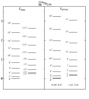
As stated above, the isotope 224Th is one of the best candidates for research on “pear shape” deformation. Its low energy spectrum has been studied previously in [22] where a Hamiltonian involving the Casimir operators of orders two and three was formulated. In this section we take the Hamiltonian in 6 and use equation 7 to calculate its matrix elements which are degenerate with respect to the total angular momentum projection . The harmonic oscillator strength has the value of MeV.
This isotope has 16 particles in the valence shell; 8 protons and 8 neutrons which allow for the formation of 4 quartets. Thus, its ground state is given by the spatial representation . The reduction is given by the leading [33] irreps which couple to a leading . The band contained in this irrep corresponds to the ground state band observed experimentally. As explained above, the excited state has two contributions; the proton excitation given by and the neutron excitation given by . The reductions are the leading and respectively, both of which couple to total leading . The band contained in this irrep corresponds to the octupole excited band observed experimentally.
The Hamiltonian matrix elements to be calculated are those between the states observed experimentally which can be used to fit the parameters and . The ground state band has angular momentum and those of the excited band are . They are a total of 28 states distinguishing between the proton and neutron excited states. The intermediate states of equation 7 are too many to consider them all in a realistic calculation, thus we propose a truncation of the full model space to the ground and excited bands and . These are a total of 97 intermediate states, even though not all of them will contribute because many will cancel the one-body RME due to angular momentum selection rules. Adopting these restrictions, there will be 37 non-zero independent matrix elements of the Hamiltonian, 9 of which are non-diagonal. In this restricted space the products and will contribute to the diagonal terms while the and will form the non-diagonal matrix elements. These matrix elements are shown in appendix B.
The Elliott Hamiltonian fit to 224Th spectrum results in a quadrupole-quadrupole interaction strength of and a mean square error (MSE) of 0.1771 MeV2 to the experimental energy levels. The two-parameter Hamiltonian proposed in [22] obtains an improvement with a MSE of 0.1180 MeV2. The states of the negative parity band have two contributions from the model, taken into account as a superposition , where the proton and neutron excited states are denoted as , respectively and the parameter expresses the contribution of each nucleon type wavefunction to the total nuclear wavefunction. While the matrix elements of the ground state band are diagonal, the energy of the negative parity band states are be given by
| (8) | ||||
Computer codes were developed to calculate these Hamiltonian expectation values and fit its three parameters resulting in , and . It is equivalent to a simultaneous diagonalization and fit of the parameters. This model has a MSE of 0.1739 MeV2 and its spectrum is shown in figure 3.
VI Strength
Using the scheme and equations shown above, we can study the electromagnetic transition strength. The electric octupole transition operator is [34]
| (9) |
where the harmonic oscillator amplitude parameter is fm, the proton and neutron effective charges are and respectively. The reduced transition probability is be given by
| (10) |
with the reduced matrix element
| (11) | ||||
where represents the excited state of nucleon according to the scheme of equation 2, parameters , involve the effective charges and superposition parameter in the total excited state as and [23]. Recall that the latest evaluated experimental values of the transition are shown in figure 2
From the collective model the following relation can be demonstrated [9, 35]
| (12) |
using the experimental value for quadrupole deformation [24], the calculation for octupole deformation [36] for 224Th and the approximation for the nuclear radius fm, results in a transition strength of 77.6001 W.u. This value is close to the one reported in [37, 38] by different methods.
Assuming according to the results in [23] and considering the collective transition strength, one can estimate the value of . Under these assumptions and the value for obtained in the previous section, minimums for and are set in the model. A direct measurement of the transition for 224Th is required for further analysis.
VII CONCLUSIONS
We obtained the mathematical form of the octupole operator in terms of tensors for the actinide region which is minimally defined in the shells 5,6 in the proton space and 6,7 in the neutron space. The scalar operator is constructed from this expansion and its reduced matrix elements in the two-shell states formalism are computed in terms of products of recoupling coefficients and single-shell reduced matrix elements. Computer codes were developed that integrate several libraries [39, 40, 41, 28] in order to perform the calculations of this work. These are available under request to the authors. Essential algebraic expressions for this work are presented in appendix A along with identities used to check the computer codes developed.
The Hamiltonian proposed carries three parameters and that account for the strength of the quadrupole, octupole residual interactions and nucleon contributions respectively. This model was applied to the low-lying spectrum of the isotope 224Th obtaining a slight improvement with respect to the original Elliott model. Increasing the number of parameters of the model would improve the fit but decrease its explanatory capabilities. A possible improvement might be achieved by a weaker truncation of the intermediate states in equation 7, for the influence of the octupole-octupole interaction is too little in this reduced space. An analysis on the transition involving previous works on collective models, density functional theory and the scheme in this article allows to estimate the octupole effective charges of the model under certain assumptions, however, the lack of experimental data is challenging for this theoretical aspect. We hope to motivate research on this isotope from the experimental side as well.
The octupole deformation of nuclei is a research area that will help physicists obtain a better understanding of the nuclear structure and gain insight of the fundamental symmetries of nature. With this work, we expect to increase interest in this topic from the -symmetry based models and await the results of experimental efforts from novel radioactive beams accelerators which will allow the exploration of previously inaccessible nuclei.
Acknowledgements.
We would like to thank professors J. G. Hirsch, V. K. B. Kota, D. Langr and J. Cseh for very valuable discussions. We thank the Institute of Physics at University of Antioquia for supporting this research.Appendix A one-body triple-barred reduced matrix elements in two-shell states
The one-body double-barred reduced matrix elements (RME) of equation 7 can be computed with equation 10 of reference [32], which separates the proton an neutron spaces obtaining a mathematical expression in terms of recoupling coefficients and triple-barred RME. The former can be computed by libraries [40] while the latter require an additional mathematical calculation.
The proton and neutron spaces are formed each by two shells; a lower shell denoted by sub-index and an upper one denoted by sub-index , with the creation an destruction operators acting on different quantum numbers. A separation of these two shells [42] can be performed as shown in equation 16 where two situations can happen; creates a particle in the shell and destroys a particle in shell, or creates a particle in the shell and destroys a particle in shell . The first case is a de-excitation of the nucleus while the second is an excitation process. These two cases will imply a minimal change in their mathematical expressions which are distinguished with the labels and as follows: and identify the de-excitation process and and identifies the excitation process as indicated in 16. The triple-barred RME appearing on the right hand side of equation 16 are in a single shell which can be evaluated using computer packages [41, 43]. A computer program was developed to perform the calculation of equation 16 depending on the case as explained above. The following relation is useful
|
({a†(η’0)12~a(0η)12}ρ0=1,(λ0μ0),Ko,Lo,S0MLo,MSo)†= (-1)η-η’-Lo-MLo-MSo{a†(η0)12~a(0η’)12}ρ0=1,(λ0μ0),Ko,Lo,S0-MLo,-MSo, |
(13) |
and the next identities [44, 30] must be hold which were used to check the computer codes
|
⟨L’, S’—— TLo, So—— L,S⟩= (-1)L-L’+S-S’(2L+1)(2S+1)(2L’+1)(2S’+1)⟨L,S——TLo, So—— L’,S’⟩*, |
(14) |
|
⟨(λ1,μ1)———T(μ2,λ2)———(λ3,μ3)⟩⟨(λ3,μ3)———T(λ2,μ2)———(λ1,μ1)⟩=(-1)12(μ1+μ2-μ3-λ1-λ2+λ3)dim(λ3,μ3)dim(λ1,μ1). |
(15) |
|
⟨[f’-]⊗[f’+],(λ’-μ’-)⊗(λ’+μ’+),ρ’(λ’μ’),S’——— {a†(η’0)12~a(0η)12}ρ0=1,(λ0μ0)S0———[f-]⊗[f+],(λ-μ-)⊗(λ+μ+),ρ(λμ),S⟩¯ρ= {(λ-,μ-) (α, β) (λ’-,μ’-) ρ=1(λ+,μ+) (γ,δ) (λ’+,μ’+) ρ=1(λ,μ) (λo,μo) (λ’,μ’) ¯ρρρ=1 ρ’}χ{S-12S’-S+12S’+S SoS’ }(-1)ϕdim(λsμs)dim(λ’sμ’s)2Ss+12S’s+1×⟨[f’t],(λ’tμ’t),S’t———a†(η’0)12——— [ft],(λtμt)St⟩ρ=1⟨[fs],(λsμs),Ss———a†(η0)12———[f’s],(λ’sμ’s),S’s⟩ρ=1, |
(16) |
Appendix B matrix elements
| 4.5946 | 0 | 0 | 0 | 0 | 0 | 0 | 0 | 0 | 0 | 0 | 0 | 0 | 0 | 0 | 0 | 0 | 0 | 0 | 0 | 0 | 0 | 0 | 0 | 0 | 0 | 0 | 0 | |
| 0 | 25.8974 | 0 | 0 | 0 | 0 | 0 | 0 | 0 | 0 | 0 | 0 | 0 | 0 | 0 | 0 | 0 | 0 | 0 | 0 | 0 | 0 | 0 | 0 | 0 | 0 | 0 | 0 | |
| 0 | 0 | 36.6437 | 0 | 0 | 0 | 0 | 0 | 0 | 0 | 0 | 0 | 0 | 0 | 0 | 0 | 0 | 0 | 0 | 0 | 0 | 0 | 0 | 0 | 0 | 0 | 0 | 0 | |
| 0 | 0 | 0 | 32.0281 | 0 | 0 | 0 | 0 | 0 | 0 | 0 | 0 | 0 | 0 | 0 | 0 | 0 | 0 | 0 | 0 | 0 | 0 | 0 | 0 | 0 | 0 | 0 | 0 | |
| 0 | 0 | 0 | 0 | 30.4360 | 0 | 0 | 0 | 0 | 0 | 0 | 0 | 0 | 0 | 0 | 0 | 0 | 0 | 0 | 0 | 0 | 0 | 0 | 0 | 0 | 0 | 0 | 0 | |
| 0 | 0 | 0 | 0 | 0 | 29.4780 | 0 | 0 | 0 | 0 | 0 | 0 | 0 | 0 | 0 | 0 | 0 | 0 | 0 | 0 | 0 | 0 | 0 | 0 | 0 | 0 | 0 | 0 | |
| 0 | 0 | 0 | 0 | 0 | 0 | 28.8096 | 0 | 0 | 0 | 0 | 0 | 0 | 0 | 0 | 0 | 0 | 0 | 0 | 0 | 0 | 0 | 0 | 0 | 0 | 0 | 0 | 0 | |
| 0 | 0 | 0 | 0 | 0 | 0 | 0 | 28.3865 | 0 | 0 | 0 | 0 | 0 | 0 | 0 | 0 | 0 | 0 | 0 | 0 | 0 | 0 | 0 | 0 | 0 | 0 | 0 | 0 | |
| 0 | 0 | 0 | 0 | 0 | 0 | 0 | 0 | 28.2491 | 0 | 0 | 0 | 0 | 0 | 0 | 0 | 0 | 0 | 0 | 0 | 0 | 0 | 0 | 0 | 0 | 0 | 0 | 0 | |
| 0 | 0 | 0 | 0 | 0 | 0 | 0 | 0 | 0 | 28.4693 | 0 | 0 | 0 | 0 | 0 | 0 | 0 | 0 | 0 | 0 | 0 | 0 | 0 | 0 | 0 | 0 | 0 | 0 | |
| 0 | 0 | 0 | 0 | 0 | 0 | 0 | 0 | 0 | 0 | 0.0583 | 0 | 0 | 0 | 0 | 0 | 0 | 0 | 0 | 0.8057 | 0 | 0 | 0 | 0 | 0 | 0 | 0 | 0 | |
| 0 | 0 | 0 | 0 | 0 | 0 | 0 | 0 | 0 | 0 | 0 | 0.8027 | 0 | 0 | 0 | 0 | 0 | 0 | 0 | 0 | 5.8653 | 0 | 0 | 0 | 0 | 0 | 0 | 0 | |
| 0 | 0 | 0 | 0 | 0 | 0 | 0 | 0 | 0 | 0 | 0 | 0 | 0.7432 | 0 | 0 | 0 | 0 | 0 | 0 | 0 | 0 | 3.9895 | 0 | 0 | 0 | 0 | 0 | 0 | |
| 0 | 0 | 0 | 0 | 0 | 0 | 0 | 0 | 0 | 0 | 0 | 0 | 0 | 1.0362 | 0 | 0 | 0 | 0 | 0 | 0 | 0 | 0 | 4.1776 | 0 | 0 | 0 | 0 | 0 | |
| 0 | 0 | 0 | 0 | 0 | 0 | 0 | 0 | 0 | 0 | 0 | 0 | 0 | 0 | 1.4556 | 0 | 0 | 0 | 0 | 0 | 0 | 0 | 0 | 4.6520 | 0 | 0 | 0 | 0 | |
| 0 | 0 | 0 | 0 | 0 | 0 | 0 | 0 | 0 | 0 | 0 | 0 | 0 | 0 | 0 | 1.9908 | 0 | 0 | 0 | 0 | 0 | 0 | 0 | 0 | 5.2846 | 0 | 0 | 0 | |
| 0 | 0 | 0 | 0 | 0 | 0 | 0 | 0 | 0 | 0 | 0 | 0 | 0 | 0 | 0 | 0 | 2.6439 | 0 | 0 | 0 | 0 | 0 | 0 | 0 | 0 | 6.0400 | 0 | 0 | |
| 0 | 0 | 0 | 0 | 0 | 0 | 0 | 0 | 0 | 0 | 0 | 0 | 0 | 0 | 0 | 0 | 0 | 3.4203 | 0 | 0 | 0 | 0 | 0 | 0 | 0 | 0 | 6.9057 | 0 | |
| 0 | 0 | 0 | 0 | 0 | 0 | 0 | 0 | 0 | 0 | 0 | 0 | 0 | 0 | 0 | 0 | 0 | 0 | 4.3272 | 0 | 0 | 0 | 0 | 0 | 0 | 0 | 0 | 7.8818 | |
| 0 | 0 | 0 | 0 | 0 | 0 | 0 | 0 | 0 | 0 | 0.8057 | 0 | 0 | 0 | 0 | 0 | 0 | 0 | 0 | 12.7929 | 0 | 0 | 0 | 0 | 0 | 0 | 0 | 0 | |
| 0 | 0 | 0 | 0 | 0 | 0 | 0 | 0 | 0 | 0 | 0 | 5.8653 | 0 | 0 | 0 | 0 | 0 | 0 | 0 | 0 | 50.6621 | 0 | 0 | 0 | 0 | 0 | 0 | 0 | |
| 0 | 0 | 0 | 0 | 0 | 0 | 0 | 0 | 0 | 0 | 0 | 0 | 3.9895 | 0 | 0 | 0 | 0 | 0 | 0 | 0 | 0 | 32.9312 | 0 | 0 | 0 | 0 | 0 | 0 | |
| 0 | 0 | 0 | 0 | 0 | 0 | 0 | 0 | 0 | 0 | 0 | 0 | 0 | 4.1776 | 0 | 0 | 0 | 0 | 0 | 0 | 0 | 0 | 29.9974 | 0 | 0 | 0 | 0 | 0 | |
| 0 | 0 | 0 | 0 | 0 | 0 | 0 | 0 | 0 | 0 | 0 | 0 | 0 | 0 | 4.6520 | 0 | 0 | 0 | 0 | 0 | 0 | 0 | 0 | 28.2286 | 0 | 0 | 0 | 0 | |
| 0 | 0 | 0 | 0 | 0 | 0 | 0 | 0 | 0 | 0 | 0 | 0 | 0 | 0 | 0 | 5.2846 | 0 | 0 | 0 | 0 | 0 | 0 | 0 | 0 | 26.7378 | 0 | 0 | 0 | |
| 0 | 0 | 0 | 0 | 0 | 0 | 0 | 0 | 0 | 0 | 0 | 0 | 0 | 0 | 0 | 0 | 6.0400 | 0 | 0 | 0 | 0 | 0 | 0 | 0 | 0 | 25.3676 | 0 | 0 | |
| 0 | 0 | 0 | 0 | 0 | 0 | 0 | 0 | 0 | 0 | 0 | 0 | 0 | 0 | 0 | 0 | 0 | 6.9057 | 0 | 0 | 0 | 0 | 0 | 0 | 0 | 0 | 24.1192 | 0 | |
| 0 | 0 | 0 | 0 | 0 | 0 | 0 | 0 | 0 | 0 | 0 | 0 | 0 | 0 | 0 | 0 | 0 | 0 | 7.8818 | 0 | 0 | 0 | 0 | 0 | 0 | 0 | 0 | 23.0470 |
References
- Heyde and Wood [2016] K. Heyde and J. L. Wood, Nuclear shapes: from earliest ideas to multiple shape coexisting structures, Physica Scripta 91, 083008 (2016).
- Mackintosh [1977] R. S. Mackintosh, The shape of nuclei, Reports on Progress in Physics 40, 731 (1977).
- Nilsson and Ragnarsson [1995] S. Nilsson and I. Ragnarsson, Shapes and Shells in Nuclear Structure (Cambridge University Press, 1995).
- Tajima and Suzuki [2001] N. Tajima and N. Suzuki, Prolate dominance of nuclear shape caused by a strong interference between the effects of spin-orbit and terms of the nilsson potential, Phys. Rev. C 64, 037301 (2001).
- Heyde and Wood [2011] K. Heyde and J. L. Wood, Shape coexistence in atomic nuclei, Rev. Mod. Phys. 83, 1467 (2011).
- Martinou et al. [2021] A. Martinou, D. Bonatsos, T. J. Mertzimekis, K. E. Karakatsanis, I. E. Assimakis, S. K. Peroulis, S. Sarantopoulou, and N. Minkov, The islands of shape coexistence within the elliott and the proxy-SU(3) models, The European Physical Journal A 57, 84 (2021).
- Stone [2016] N. Stone, Table of nuclear electric quadrupole moments, Atomic Data and Nuclear Data Tables 111-112, 1 (2016).
- Bonatsos et al. [2017a] D. Bonatsos, I. E. Assimakis, N. Minkov, A. Martinou, S. Sarantopoulou, R. B. Cakirli, R. F. Casten, and K. Blaum, Analytic predictions for nuclear shapes, prolate dominance, and the prolate-oblate shape transition in the proxy-su(3) model, Phys. Rev. C 95, 064326 (2017a).
- Butler [2016] P. A. Butler, Octupole collectivity in nuclei, Journal of Physics G: Nuclear and Particle Physics 43, 073002 (2016).
- Ahmad and Butler [1993] I. Ahmad and P. A. Butler, Octupole shapes in nuclei, Annual Review of Nuclear and Particle Science 43, 71 (1993).
- Butler and Nazarewicz [1996] P. A. Butler and W. Nazarewicz, Intrinsic reflection asymmetry in atomic nuclei, Rev. Mod. Phys. 68, 349 (1996).
- Butler [2020] P. A. Butler, Pear-shaped atomic nuclei, Proceedings of the Royal Society A: Mathematical, Physical and Engineering Sciences 476, 20200202 (2020).
- Pancholi [2020] S. Pancholi, Pear-shaped Nuclei (World Scientific Publishing Company, 2020).
- Nomura et al. [2014] K. Nomura, D. Vretenar, T. Nikšić, and B.-N. Lu, Microscopic description of octupole shape-phase transitions in light actinide and rare-earth nuclei, Phys. Rev. C 89, 024312 (2014).
- Pospelov and Ritz [2005] M. Pospelov and A. Ritz, Electric dipole moments as probes of new physics, Annals of Physics 318, 119 (2005), special Issue.
- Griffith et al. [2009] W. C. Griffith, M. D. Swallows, T. H. Loftus, M. V. Romalis, B. R. Heckel, and E. N. Fortson, Improved limit on the permanent electric dipole moment of , Phys. Rev. Lett. 102, 101601 (2009).
- Gaffney et al. [2013] L. P. Gaffney, P. A. Butler, M. Scheck, A. B. Hayes, F. Wenander, M. Albers, B. Bastin, C. Bauer, A. Blazhev, S. Bönig, N. Bree, J. Cederkäll, T. Chupp, D. Cline, T. E. Cocolios, T. Davinson, H. De Witte, J. Diriken, T. Grahn, A. Herzan, M. Huyse, D. G. Jenkins, D. T. Joss, N. Kesteloot, J. Konki, M. Kowalczyk, T. Kröll, E. Kwan, R. Lutter, K. Moschner, P. Napiorkowski, J. Pakarinen, M. Pfeiffer, D. Radeck, P. Reiter, K. Reynders, S. V. Rigby, L. M. Robledo, M. Rudigier, S. Sambi, M. Seidlitz, B. Siebeck, T. Stora, P. Thoele, P. Van Duppen, M. J. Vermeulen, M. von Schmid, D. Voulot, N. Warr, K. Wimmer, K. Wrzosek-Lipska, C. Y. Wu, and M. Zielinska, Studies of pear-shaped nuclei using accelerated radioactive beams, Nature 497, 199 (2013).
- Thorsteinsen et al. [1990] T. F. Thorsteinsen, K. Nybø, and G. Løvhøiden, Levels in 226ra populated by inelastic deuteron scattering, Physica Scripta 42, 141 (1990).
- Cseh [2015] J. Cseh, Algebraic models for shell-like quarteting of nucleons, Physics Letters B 743, 213 (2015).
- Bonatsos et al. [2017b] D. Bonatsos, I. E. Assimakis, N. Minkov, A. Martinou, R. B. Cakirli, R. F. Casten, and K. Blaum, Proxy-su(3) symmetry in heavy deformed nuclei, Phys. Rev. C 95, 064325 (2017b).
- Bonatsos et al. [2023] D. Bonatsos, A. Martinou, S. K. Peroulis, T. J. Mertzimekis, and N. Minkov, The proxy-su(3) symmetry in atomic nuclei, Symmetry 15, 10.3390/sym15010169 (2023).
- Cseh [2020] J. Cseh, Shell-like quarteting in heavy nuclei: Algebraic approaches based on the pseudo- and proxy-su(3) schemes, Phys. Rev. C 101, 054306 (2020).
- Restrepo and Valencia [2024] A. Restrepo and J. P. Valencia, Inter-band b(e1) strengths in heavy nuclei based on the proxy-su(3) scheme (2024), arXiv:2405.04679 [nucl-th] .
- [24] B. Singh and S. Singh, From ENSDF database as of March 08, 2022. Version available at http://www.nndc.bnl.gov/ensarchivals/.
- Martinou and Minkov [2024] A. Martinou and N. Minkov, Microscopic derivation of the octupole magic numbers from symmetry considerations, Physica Scripta 99, 075311 (2024).
- Isacker and Pittel [2016] P. V. Isacker and S. Pittel, Symmetries and deformations in the spherical shell model, Physica Scripta 91, 023009 (2016).
- Frank et al. [2008] A. Frank, J. Jolie, and P. van Isacker, Symmetries in Atomic Nuclei: From Isospin to Supersymmetry, Springer Tracts in Modern Physics (Springer New York, 2008).
- Draayer et al. [1989] J. Draayer, Y. Leschber, S. Park, and R. Lopez, Representations of u(3) in u(n), Computer Physics Communications 56, 279 (1989).
- Sloane [2014] F. Sloane, Lie Algebras and Applications, Lecture Notes in Physics (Springer Berlin Heidelberg, 2014).
- Vergados [1968] J. Vergados, Su(3) r(3) wigner coefficients in the 2s-1d shell, Nuclear Physics A 111, 681 (1968).
- Moshinsky and Smirnov [1996] M. Moshinsky and Y. Smirnov, The Harmonic Oscillator in Modern Physics, Contemporary concepts in physics (Harwood Academic Publishers, 1996).
- Troltenier et al. [1995] D. Troltenier, C. Bahri, and J. Draayer, Generalized pseudo-su(3) model and pairing, Nuclear Physics A 586, 53 (1995).
- Kota [2020] V. Kota, SU(3) Symmetry in Atomic Nuclei (Springer Nature Singapore, 2020).
- Brussaard and Glaudemans [1977] P. Brussaard and P. Glaudemans, Shell-model Applications in Nuclear Spectroscopy (North-Holland Publishing Company, 1977).
- Leander and Sheline [1984] G. Leander and R. Sheline, Intrinsic reflection asymmetry in odd-a nuclei, Nuclear Physics A 413, 375 (1984).
- Möller et al. [2016] P. Möller, A. Sierk, T. Ichikawa, and H. Sagawa, Nuclear ground-state masses and deformations: Frdm(2012), Atomic Data and Nuclear Data Tables 109-110, 1 (2016).
- Robledo and Butler [2013] L. M. Robledo and P. A. Butler, Quadrupole-octupole coupling in the light actinides, Phys. Rev. C 88, 051302 (2013).
- Gaffney [2012] L. P. Gaffney, Octupole collectivity in 220Rn and 224Ra, Phd thesis, University of Liverpool (2012), available at https://cds.cern.ch/record/1547569/files/CERN-THESIS-2012-309.pdf.
- Wybourne [2022] B. G. Wybourne, Schur Group Theory Software (2022).
- Dytrych et al. [2021] T. Dytrych, D. Langr, J. P. Draayer, K. D. Launey, and D. Gazda, Su3lib: A c++ library for accurate computation of wigner and racah coefficients of su(3), Computer Physics Communications 269, 108137 (2021).
- Bahri and Draayer [1994] C. Bahri and J. Draayer, Su(3) reduced matrix element package, Computer Physics Communications 83, 59 (1994).
- Millener [1991] D. J. Millener, Su(3) in shell-model calculations (1991).
- Hirsch et al. [2007] G. J. Hirsch, C. Bahri, J. Draayer, O. Castaños, and P. Hess, Reduced matrix elements for the leading spin zero states in the su ( 3 ) scheme * (2007).
- Suhonen [2007] J. Suhonen, From Nucleons to Nucleus: Concepts of Microscopic Nuclear Theory, Theoretical and Mathematical Physics (Springer Berlin Heidelberg, 2007).