Lifshitz formulas for finite-density Casimir effect
Abstract
The Lifshitz formula is well known as a theoretical approach to investigate the Casimir effect at finite temperature. In this Letter, we generalize the Lifshitz formula to the Casimir effect originating from quantum fields at finite chemical potential. To demonstrate the versatility of this formula, we discuss the typical phenomena of the Casimir effect at finite chemical potential in various systems, such as some boundary conditions, finite temperatures, arbitrary spatial dimensions, and mismatched chemical potentials. This formula can be applied to the Casimir effect in dense quark matter and Dirac/Weyl semimetals, where the chemical potential is regarded as a parameter to control the Casimir effect.
Introduction.—In 1948, Casimir predicted that the zero-point energy of photon fields in vacuum sandwiched by two perfectly conducting parallel plates induces an attractive force [1], which is the so-called Casimir effect (see Refs. [2, 3] for experiments and Refs. [4, 5, 6, 7, 8, 9] for reviews). After that, in 1956, Lifshitz derived an alternative formula [10] which is nowadays called the Lifshitz formula. This is a regularization technique to remove the divergence of the zero-point energy and reproduce Casimir’s original result. Furthermore, this formula predicts the dependence on finite temperature and/or dielectric functions of parallel plates. The study of the Casimir effect at finite temperature is practically needed because experiments for the measurement of Casimir force are, more or less, exposed to a finite-temperature environment.
Whereas the thermal Casimir effect 111Precisely speaking, “thermal” for the Casimir effect has two meanings: (i) temperature dependence of the free energy for photon fields and (ii) temperature dependence of the dielectric functions of materials composing of boundary conditions such as parallel plates. was well-established by the excellent agreement between theory [10, 12, 13, 14, 15] and experiment [16], the counterpart at finite chemical potential is still unknown. The main reason is that the conventional study of the Casimir effect focuses on the photon field, and it is usually difficult to control the chemical potential of photons in equilibrium (for non-equilibrium cases, see Refs. [17, 18]). On the other hand, if one focuses on the Casimir effect originating from fermion fields [19, 20, 21], the corresponding chemical potential can be a significant parameter to control the Casimir effect: the fermionic counterpart of the Casimir effect might be realized in quark systems and Dirac/Weyl materials, but its experimental observation is still an open problem, which requires more controllable parameters. Theoretically, an approach that correctly implements chemical potentials is needed, but it has not yet been established. In this Letter, for the first time, we extend the Lifshitz formula to systems at finite chemical potential.
Main formula.—First, we show our main finding. As a typical example, we consider the Dirac field with a mass and at chemical potential in the (3+1) dimensional spacetime. As an idealized boundary condition, we impose the periodic boundary conditions (PBCs) at and in the direction, where the momentum is discretized as . Then, the Lifshitz formula for the Casimir energy (per unit area) is written as
| (1) | ||||
| (2) |
in the natural unit of with the reduced Planck constant and the speed of light . Here, is the imaginary part of the imaginary frequency , and and are the momenta in the perpendicular direction. The overall factor of is regarded as the minus sign from the fermion zero-point energy and the particle-antiparticle and spin degrees of freedom. The form of depends on the boundary condition and is now characterized by the PBC. By substituting to this formula, we obtain the conventional Lifshitz formula.
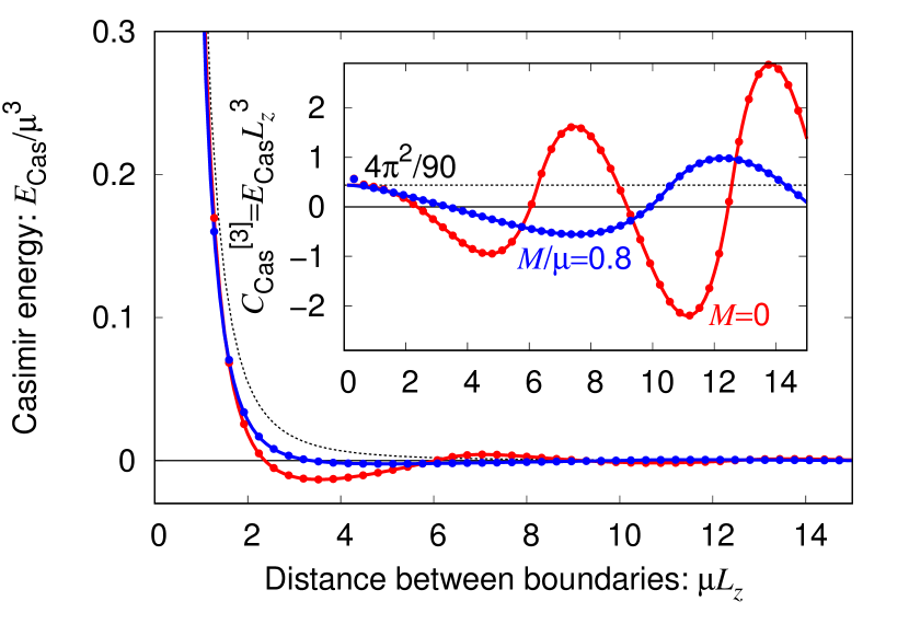
Using Eq. (1), in Fig. 1, we show a typical behavior of the Casimir energy at finite chemical potential, Here, we defined a Casimir coefficient in order to visualize the scaling well known for massless fields. For (i.e., at zero density), we obtain the conventional behavior of the Casimir effect for massless or massive fields because there is no contribution from the Fermi sea. For (i.e., at finite density), we find an oscillation of the Casimir energy as a function of . This oscillation is caused by the relationship between the fixed Fermi level and the -dependent eigenvalues discretized by boundary conditions (for a graphical explanation, see Ref. [22]). For this reason, the oscillation period is given as,
| (3) |
Using this formula, we get for the massless field, and the massive field leads to a longer period. Note that the so-called oscillating Casimir effect (or Casimir-like interaction) can be induced by various types of systems and origins (e.g., see Refs. [23, 24, 25, 26, 27, 28, 29, 30, 31, 32, 33, 17, 34, 35, 36, 37, 38, 39, 22, 18]), but Eq. (1) is regarded as a new formula containing both the non-oscillating Casimir effect at and the oscillating one at .
To check the validity of the Lifshitz formula (1), we compare with the results obtained by the lattice regularization approach [40, 41, 35, 36, 42, 43, 37, 38, 44, 39, 45, 46, 47] (see Ref. [22] at finite ). The lattice regularization can usually reproduce the correct result by taking the continuum limit () whereas at a nonzero lattice spacing () the result in the short- region deviates. In Fig. 1, we fix the lattice spacing as which is small enough. We can see that, in the longer- region, both the results well coincide, which suggests that Eq. (1) describes the correct behaviors of the Casimir effect.
Derivation.—Here, we overview a derivation of the Lifshitz formula (1). We start from the zero-point energy (i.e., the sum of eigenvalues) of the Dirac field under the PBC and finite chemical potential:
| (4) | |||
| (5) |
The overall factor of is from the fermion statistics and the spin degrees of freedom. The prime in the sum means that the factor is multiplied only for . By the argument principle 222The derivation using the argument principle is standard also at zero chemical potential [66, 67, 6]., using an integer with the Fermi momentum , the infinite sum can be evaluated as
| (6) | |||
| (7) | |||
| (8) |
The contour integral along the closed path on the complex plane consists of the infinite integral on the imaginary axis and the counterclockwise integral along on a semicircle (in the right half of the plane) with an infinite radius centered at the origin. is a meromorphic function with no pole
| (9) | |||
The zero points of in the region surrounded by are at (i.e., the eigenvalues higher than the Fermi level) on the real axis. On the other hand, the zero points of in contain as well as at (i.e., the eigenvalues lower than the Fermi level).
With the imaginary frequency , the first term of Eq. (8) vanishes because of in the limit of . Furthermore, by performing integration by parts on the second term of Eq. (8), we obtain the Lifshitz formula. Finally, because in Eq. (9) leads to the same result, we obtain the formula (1).
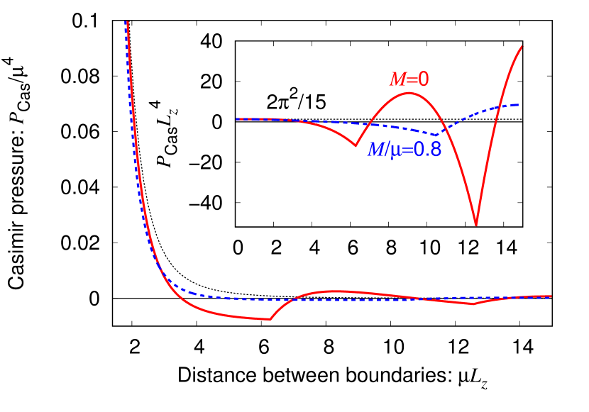
Application 1: Casimir pressure and Casimir force.—Experimentally, when the measurement of the energy difference is difficult, more realistic observables are the Casimir pressure and Casimir force. These quantities can be easily obtained from the derivative of the Casimir energy (1):
| (10) | ||||
| (11) |
These can be called the Lifshitz formula for Casimir pressure and force at finite . In Fig. 2, we show a typical behavior of the Casimir pressure. We find that, similar to the Casimir energy, the corresponding pressure and force also oscillate, but their waveforms are different from that of the Casimir energy.
Application 2: Boundary conditions.—The cases with the other boundary conditions can be derived in a similar manner. For the antiperiodic boundary conditions (APBC), the discrete momentum is given as . Then, the Lifsthiz formula is
| (12) |
The difference from Eq. (1) is only the sign in front of . Note that, the oscillation period is the same as Eq. (3) for the PBC.
Similarly, we can obtain the formula for the boundary conditions leading to , which corresponds to the MIT bag boundary conditions [49] well known for massless Dirac fields:
| (13) |
The differences from Eq. (12) are the overall factor and the exponential function . For the latter reason, the oscillation period is shorter than Eq. (3) for the PBC/APBC by a factor of : . Thus, our formulas can be applied to various boundary conditions 333Another famous boundary condition is the case leading to the discrete momentum . This situation is realized by the Dirichlet or Neumann boundaries for scalar fields and by perfectly conducting plates for photon fields. The corresponding formula is obtained by putting the minus sign in front of in Eq. (13) (and by multiplying by appropriate factors for specific quantum fields)..
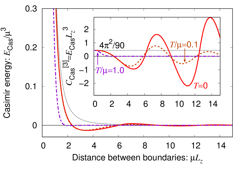
Application 3: Finite temperature.—At finite temperature, we replace the infinite integral with the infinite sum , where is the fermion Matubara frequency with the label and the temperature . Using this replacement, Eq. (1) is deformed as
| (14) | ||||
This formula contains all the dependences from the vacuum, finite , and finite . The limit is equivalent to Eq. (1) 444Also, the limit is consistent with the known formula (see, e.g., Ref. [21] for the fermionic Casimir effect at finite temperature).. In Fig. 3, we compare the results at , , and . We find a suppression of the Casimir effect due to the temperature 555 Note that the temperature dependence of the Casimir effect depends on boson or fermion fields. Since we now consider the Dirac fermion field, the total (i.e., zero-temperature plus finite-temperature) Casimir effect is suppressed as a function of temperature. On the other hand, the bosonic thermal Casimir effect is usually enhanced.
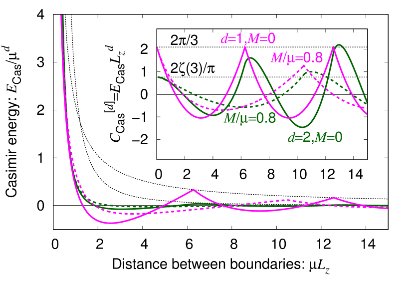
Application 4: Spatial dimensions.—The formula (1) is in the (3+1) dimensional spacetime, but it can be generalized to arbitrary (+1) dimensional spacetime by replacing as the transverse momenta and . Then,
| (15) | ||||
| (16) |
where we kept the spin degrees of freedom for simplicity. In particular, the lower dimensional ( or ) systems are realized in condensed matter physics. In Fig. 4, we show the typical behaviors of the Casimir energies and coefficients . For both and , we find oscillatory behaviors, and their periods are characterized by : the period is independent of . At , is nondifferentiable at a certain , which means that is discontinuous at the same . This is different from , where is nondifferentiable (see Fig. 2 at ). Furthermore, we find that the -dependent part of is scaled as , which is distinct from the vacuum part scaled as at . Thus, the dimensional structure of the Fermi sea (i.e., Fermi sphere, Fermi circle, and Fermi line) characterizes the typical behavior of the oscillating Casimir effect. Conversely, the measurement of the oscillatory behavior is useful as a signal of the dimensional structures of the dominant quantum fields.
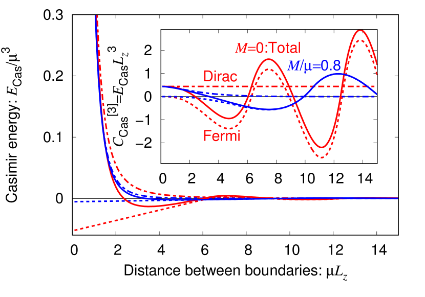
Application 5: Separation of Dirac and Fermi seas.—While Eq. (1) contains both the contributions from the zero-point energy from the -independent vacuum (the Dirac sea) and the -dependent energy (the Fermi sea), we can obtain only that from the Dirac sea by substituting . Therefore, we can also calculate only the contribution from the Fermi sea by subtracting the Dirac-sea contribution from the total Casimir energy :
| (17) |
Thus, using the combination of the Lifshitz formulas, we can describe even the contribution of the Fermi sea. In Fig. 5, we compare the total, Dirac-sea, and Fermi-sea contributions.
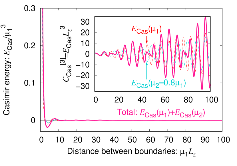
Application 6: Mismatched chemical potentials.—For two kinds of Dirac fields at different chemical potentials and , the total Casimir energy is represented as the sum of the two Casimir energies:
| (18) |
If , then the total Casimir energy is twice as large as one Casimir energy. If , the total Casimir energy oscillates as a superposition of the two oscillations, and a new period appears. This is the so-called beating Casimir effect 666This beating Casimir effect is a new phenomenon in the sense that it arises from the multiple chemical potentials. Similar beating Casimir effects were predicted from other origins: spin-split Dirac points [38] and multiple exceptional points [39]. As an example, in Fig. 6, we show the results for the two massless Dirac fields at and . Then, the period of the beat is estimated as : . Note that mismatching of two (or more) chemical potentials is not a rare situation and is frequently realized in nuclear physics: the chemical potentials of protons and neutrons in nuclear matter (or up and down quarks in quark matter) are different in environments such as neutron stars and neutron-rich nuclei.
Finally, we show some examples of physical platforms for our formulas.
Physical example 1: Quark matter.—We emphasize that Eq. (1) is a standard formula for the Dirac field at finite chemical potential, and such a situation is realistic for quark fields in dense quark matter. Since the free up and down quarks are approximately massless and their velocity is close to the speed of light, the magnitude of the Casimir energy can be comparable with the photonic one and is enhanced by the factors of flavors and colors. In particular, a thin domain of dense quark matter [22] or quark-gluon plasma [54, 55, 56] is regarded as the Casimir effect-like geometry. Dynamics of interacting quarks is described by quantum chromodynamics (QCD). Its nonperturbative analysis is difficult, but effective models based on a quasiparticle picture of quarks can be utilized. Our formulas will be useful in various types of effective models of quasiquarks. The Casimir effect in dense QCD (or effective models of dense quark matter) will be preciously examined by numerical lattice simulations (free from the sign problem). Recently, because lattice simulations of the Casimir effect for Yang-Mills fields are vigorously developed [57, 58, 59, 60], the comprehensive study including quark fields is an urgent issue.
Physical example 2: Dirac/Weyl semimetals.—Similar to quark matter, (three-dimensional) Dirac or Weyl semimetals [61] are another testing ground for the Casimir effect originating from Dirac or Weyl electron fields. In particular, thin films of these materials are regarded as the Casimir effect-like geometry [38]. Then, the typical magnitude of the fermionic Casimir effect is characterized by the Fermi velocity (typically, -% of the speed of light), but its contribution is relevant as a part of thermodynamics inside materials. Experimentally, the chemical potential (i.e., the position of the Fermi level) in these materials can be controlled by doping electrons [62] or applying gate voltages [63], which means that the -dependent Casimir effect can also be controlled. Our formulas will be useful for various types of effective Hamiltonians to describe Dirac/Weyl semimetals.
Physical example 3: lower-dimensional materials.—In the case of two-dimensional Dirac fermions, as described by in the formula (15), promising systems are Dirac electrons living on graphene and surface states on topological insulators [36]. In particular, carbon nanotubes can be regarded as a platform of the electronic Casimir effect with the PBC [64, 65].
Conclusion.—In this Letter, we focused on the Lifshitz formulas for the Dirac fermions at finite chemical potential and its application. Similarly, the formulas for bosonic fields, such as charged scalar and gauge fields, will be straightforward. If bosonic chemical potentials are experimentally controllable, the corresponding formulas will be significant tools.
Acknowledgments—This work was supported by the Japan Society for the Promotion of Science (JSPS) KAKENHI (Grants No. JP20K14476, JP24K07034, JP24K17054, JP24K17059).
References
- Casimir [1948] H. B. G. Casimir, On the Attraction Between Two Perfectly Conducting Plates, Proc. Kon. Ned. Akad. Wetensch. 51, 793 (1948).
- Lamoreaux [1997] S. K. Lamoreaux, Demonstration of the Casimir Force in the 0.6 to Range, Phys. Rev. Lett. 78, 5 (1997), [Erratum: Phys. Rev. Lett. 81, 5475 (1998)].
- Bressi et al. [2002] G. Bressi, G. Carugno, R. Onofrio, and G. Ruoso, Measurement of the Casimir force between parallel metallic surfaces, Phys. Rev. Lett. 88, 041804 (2002), arXiv:quant-ph/0203002 .
- Plunien et al. [1986] G. Plunien, B. Müller, and W. Greiner, The Casimir Effect, Phys. Rep. 134, 87 (1986).
- Mostepanenko and Trunov [1988] V. M. Mostepanenko and N. N. Trunov, The Casimir Effect and Its Applications, Sov. Phys. Usp. 31, 965 (1988).
- Bordag et al. [2001] M. Bordag, U. Mohideen, and V. M. Mostepanenko, New developments in the Casimir effect, Phys. Rep. 353, 1 (2001), arXiv:quant-ph/0106045 [quant-ph] .
- Milton [2001] K. A. Milton, The Casimir Effect: Physical Manifestations of Zero-Point Energy (World Scientific, Singapore, 2001).
- Klimchitskaya et al. [2009] G. L. Klimchitskaya, U. Mohideen, and V. M. Mostepanenko, The Casimir force between real materials: Experiment and theory, Rev. Mod. Phys. 81, 1827 (2009), arXiv:0902.4022 [cond-mat.other] .
- Gong et al. [2021] T. Gong, M. R. Corrado, A. R. Mahbub, C. Shelden, and J. N. Munday, Recent progress in engineering the Casimir effect – applications to nanophotonics, nanomechanics, and chemistry, Nanophotonics 10, 523 (2021).
- Lifshitz [1956] E. M. Lifshitz, The theory of molecular attractive forces between solids, Sov. Phys. JETP 2, 73 (1956).
- Note [1] Precisely speaking, “thermal” for the Casimir effect has two meanings: (i) temperature dependence of the free energy for photon fields and (ii) temperature dependence of the dielectric functions of materials composing of boundary conditions such as parallel plates.
- Fierz [1960] M. Fierz, On the attraction of conducting planes in vacuum, Helv. Phys. Acta 33, 855 (1960).
- Mehra [1967] J. Mehra, Temperature correction to the Casimir effect, Physica 37, 145 (1967).
- Brown and Maclay [1969] L. S. Brown and G. J. Maclay, Vacuum stress between conducting plates: An Image solution, Phys. Rev. 184, 1272 (1969).
- Schwinger et al. [1979] J. S. Schwinger, L. L. DeRaad, Jr., and K. A. Milton, Casimir Effect in Dielectrics, Annals Phys. 115, 1 (1979).
- Sushkov et al. [2011] A. O. Sushkov, W. J. Kim, D. A. R. Dalvit, and S. K. Lamoreaux, Observation of the thermal Casimir force, Nature Phys. 7, 230 (2011), arXiv:1011.5219 [quant-ph] .
- Chen and Fan [2016] K. Chen and S. Fan, Nonequilibrium Casimir Force with a Nonzero Chemical Potential for Photons, Phys. Rev. Lett. 117, 267401 (2016).
- [18] B. Spreng, C. Shelden, T. Gong, and J. N. Munday, Casimir repulsion with biased semiconductors, arXiv:2403.09007 [quant-ph] .
- Johnson [1975] K. Johnson, The M.I.T. Bag Model, Acta Phys. Polon. B 6, 865 (1975).
- Mamaev and Trunov [1980] S. G. Mamaev and N. N. Trunov, Vacuum expectation values of the energy-momentum tensor of quantized fields on manifolds with different topologies and geometries. III, Sov. Phys. J. 23, 551 (1980).
- Gundersen and Ravndal [1988] S. A. Gundersen and F. Ravndal, The fermionic Casimir effect at finite temperature, Annals Phys. 182, 90 (1988).
- Fujii et al. [2024] D. Fujii, K. Nakayama, and K. Suzuki, Dual chiral density wave induced oscillating Casimir effect, Phys. Rev. D 110, 014039 (2024), arXiv:2402.17638 [hep-ph] .
- Bulgac and Wirzba [2001] A. Bulgac and A. Wirzba, Casimir interaction among objects immersed in a fermionic environment, Phys. Rev. Lett. 87, 120404 (2001), arXiv:nucl-th/0102018 .
- Fuchs et al. [2007] J. N. Fuchs, A. Recati, and W. Zwerger, Oscillating Casimir force between impurities in one-dimensional Fermi liquids, Phys. Rev. A 75, 043615 (2007), arXiv:cond-mat/0610659 [cond-mat.mes-hall] .
- Wächter et al. [2007] P. Wächter, V. Meden, and K. Schönhammer, Indirect forces between impurities in one-dimensional quantum liquids, Phys. Rev. B 76, 045123 (2007), arXiv:cond-mat/0703128 [cond-mat.str-el] .
- Kolomeisky et al. [2008] E. B. Kolomeisky, J. P. Straley, and M. Timmins, Casimir effect in a one-dimensional gas of free fermions, Phys. Rev. A 78, 022104 (2008), arXiv:0706.2887 [cond-mat.mes-hall] .
- Nishida [2009] Y. Nishida, Casimir interaction among heavy fermions in the BCS-BEC crossover, Phys. Rev. A 79, 013629 (2009), arXiv:0811.1615 [cond-mat.other] .
- Zhabinskaya and Mele [2009] D. Zhabinskaya and E. J. Mele, Casimir interactions between scatterers in metallic carbon nanotubes, Phys. Rev. B 80, 155405 (2009), arXiv:0909.1731 [cond-mat.mes-hall] .
- Chen et al. [2012] L.-W. Chen, G.-Z. Su, J.-C. Chen, and A. Bjarne, Oscillating Casimir force between two slabs in a Fermi sea, Chin. Phys. B 21, 010501 (2012).
- Chen et al. [2011] L. Chen, G. Su, and J. Chen, Oscillating Casimir effect of a trapped Fermi gas, J. Stat. Phys. 143, 523 (2011).
- Krüger et al. [2011] M. Krüger, T. Emig, G. Bimonte, and M. Kardar, Non-equilibrium Casimir forces: Spheres and sphere-plate, EPL 95, 21002 (2011), arXiv:1105.5577 [quant-ph] .
- Krüger et al. [2012] M. Krüger, G. Bimonte, T. Emig, and M. Kardar, Trace formulae for non-equilibrium Casimir interactions, heat radiation and heat transfer for arbitrary objects, Phys. Rev. B 86, 115423 (2012), arXiv:1207.0374 [quant-ph] .
- [33] A. Han, Seyit Deniz and E. Aydiner, Oscillating Casimir force of trapped Bose gas in electromagnetic field, arXiv:1508.01040 [quant-ph] .
- Jiang and Wilczek [2019] Q.-D. Jiang and F. Wilczek, Chiral Casimir forces: Repulsive, enhanced, tunable, Phys. Rev. B 99, 125403 (2019), arXiv:1805.07994 [cond-mat.mes-hall] .
- Ishikawa et al. [2020] T. Ishikawa, K. Nakayama, and K. Suzuki, Casimir effect for lattice fermions, Phys. Lett. B 809, 135713 (2020), arXiv:2005.10758 [hep-lat] .
- Ishikawa et al. [2021] T. Ishikawa, K. Nakayama, and K. Suzuki, Lattice-fermionic Casimir effect and topological insulators, Phys. Rev. Res. 3, 023201 (2021), arXiv:2012.11398 [hep-lat] .
- Mandlecha and Gavai [2022] Y. V. Mandlecha and R. V. Gavai, Lattice fermionic Casimir effect in a slab bag and universality, Phys. Lett. B 835, 137558 (2022), arXiv:2207.00889 [hep-lat] .
- Nakayama and Suzuki [2023a] K. Nakayama and K. Suzuki, Dirac/Weyl-node-induced oscillating Casimir effect, Phys. Lett. B 843, 138017 (2023a), arXiv:2207.14078 [cond-mat.mes-hall] .
- Nakata and Suzuki [2024] K. Nakata and K. Suzuki, Non-Hermitian Casimir effect of magnons, npj Spintronics 2, 11 (2024), arXiv:2305.09231 [quant-ph] .
- Actor et al. [2000] A. Actor, I. Bender, and J. Reingruber, Casimir effect on a finite lattice, Fortsch. Phys. 48, 303 (2000), arXiv:quant-ph/9908058 [quant-ph] .
- [41] M. Pawellek, Finite-sites corrections to the Casimir energy on a periodic lattice, arXiv:1303.4708 [hep-th] .
- Nakayama and Suzuki [2023b] K. Nakayama and K. Suzuki, Remnants of the nonrelativistic Casimir effect on the lattice, Phys. Rev. Res. 5, L022054 (2023b), arXiv:2204.12032 [quant-ph] .
- Nakata and Suzuki [2023] K. Nakata and K. Suzuki, Magnonic Casimir Effect in Ferrimagnets, Phys. Rev. Lett. 130, 096702 (2023), arXiv:2205.13802 [quant-ph] .
- Swingle and Van Raamsdonk [2023] B. Swingle and M. Van Raamsdonk, Enhanced negative energy with a massless Dirac field, JHEP 08, 183, arXiv:2212.02609 [hep-th] .
- [45] E. Flores, C. Ireland, N. Jamhour, V. Lasasso, N. Kurth, and M. Leinbach, Casimir force in discrete scalar fields I: 1D and 2D cases, arXiv:2309.00624 [quant-ph] .
- Nakayama and Suzuki [2024] K. Nakayama and K. Suzuki, Casimir effect in axion electrodynamics with lattice regularizations, Phys. Rev. D 109, 065002 (2024), arXiv:2310.18092 [hep-th] .
- Beenakker [2024] C. W. J. Beenakker, Topologically protected Casimir effect for lattice fermions, Phys. Rev. Res. 6, 023058 (2024), arXiv:2402.02477 [quant-ph] .
- Note [2] The derivation using the argument principle is standard also at zero chemical potential [66, 67, 6].
- Chodos et al. [1974] A. Chodos, R. L. Jaffe, K. Johnson, C. B. Thorn, and V. F. Weisskopf, A new extended model of hadrons, Phys. Rev. D 9, 3471 (1974).
- Note [3] Another famous boundary condition is the case leading to the discrete momentum . This situation is realized by the Dirichlet or Neumann boundaries for scalar fields and by perfectly conducting plates for photon fields. The corresponding formula is obtained by putting the minus sign in front of in Eq. (13) (and by multiplying by appropriate factors for specific quantum fields).
- Note [4] Also, the limit is consistent with the known formula (see, e.g., Ref. [21] for the fermionic Casimir effect at finite temperature).
- Note [5] Note that the temperature dependence of the Casimir effect depends on boson or fermion fields. Since we now consider the Dirac fermion field, the total (i.e., zero-temperature plus finite-temperature) Casimir effect is suppressed as a function of temperature. On the other hand, the bosonic thermal Casimir effect is usually enhanced.
- Note [6] This beating Casimir effect is a new phenomenon in the sense that it arises from the multiple chemical potentials. Similar beating Casimir effects were predicted from other origins: spin-split Dirac points [38] and multiple exceptional points [39].
- Hashimoto [1985] T. Hashimoto, QCD Casimir effects with bag boundary at finite temperature, Prog. Theor. Phys. 73, 1223 (1985).
- Jackson et al. [1986] A. Jackson, S. Lee, M. Prakash, and T. H. Hansson, Thermodynamics of quarks and gluons in a slab, Phys. Lett. B 182, 226 (1986).
- Saito [1991] K. Saito, Casimir effect on quark gluon plasma, Z. Phys. C 50, 69 (1991).
- Chernodub et al. [2018] M. N. Chernodub, V. A. Goy, A. V. Molochkov, and H. H. Nguyen, Casimir Effect in Yang-Mills Theory in , Phys. Rev. Lett. 121, 191601 (2018), arXiv:1805.11887 [hep-lat] .
- Chernodub et al. [2019] M. N. Chernodub, V. A. Goy, and A. V. Molochkov, Phase structure of lattice Yang-Mills theory on , Phys. Rev. D 99, 074021 (2019), arXiv:1811.01550 [hep-lat] .
- Kitazawa et al. [2019] M. Kitazawa, S. Mogliacci, I. Kolbé, and W. A. Horowitz, Anisotropic pressure induced by finite-size effects in SU(3) Yang-Mills theory, Phys. Rev. D 99, 094507 (2019), arXiv:1904.00241 [hep-lat] .
- Chernodub et al. [2023] M. N. Chernodub, V. A. Goy, A. V. Molochkov, and A. S. Tanashkin, Boundary states and non-Abelian Casimir effect in lattice Yang-Mills theory, Phys. Rev. D 108, 014515 (2023), arXiv:2302.00376 [hep-lat] .
- Armitage et al. [2018] N. P. Armitage, E. J. Mele, and A. Vishwanath, Weyl and Dirac Semimetals in Three Dimensional Solids, Rev. Mod. Phys. 90, 015001 (2018), arXiv:1705.01111 [cond-mat.str-el] .
- Liu et al. [2014] Z. K. Liu, J. Jiang, B. Zhou, Z. J. Wang, Y. Zhang, H. M. Weng, D. Prabhakaran, S.-K. Mo, H. Peng, P. Dudin, T. Kim, M. Hoesch, Z. Fang, X. Dai, Z. X. Shen, D. L. Feng, Z. Hussain, and Y. L. Chen, A stable three-dimensional topological Dirac semimetal , Nature Mater. 13, 677 (2014).
- Liu et al. [2015] Y. Liu, C. Zhang, X. Yuan, T. Lei, C. Wang, D. D. Sante, A. Narayan, L. He, S. Picozzi, S. Sanvito, R. Che, and F. Xiu, Gate-tunable quantum oscillations in ambipolar thin films, NPG Asia Mater 7, e22 (2015), arXiv:1412.4380 [cond-mat.mtrl-sci] .
- Bellucci and Saharian [2009a] S. Bellucci and A. A. Saharian, Fermionic Casimir densities in toroidally compactified spacetimes with applications to nanotubes, Phys. Rev. D 79, 085019 (2009a), arXiv:0902.3726 [hep-th] .
- Bellucci and Saharian [2009b] S. Bellucci and A. A. Saharian, Fermionic Casimir effect for parallel plates in the presence of compact dimensions with applications to nanotubes, Phys. Rev. D 80, 105003 (2009b), arXiv:0907.4942 [hep-th] .
- Van Kampen et al. [1968] N. G. Van Kampen, B. R. A. Nijboer, and K. Schram, On the macroscopic theory of Van der Waals forces, Phys. Lett. A 26, 307 (1968).
- Schram [1973] K. Schram, On the macroscopic theory of retarded Van der Waals forces, Phys. Lett. A 43, 282 (1973).