Quantum Buffer Design Using Petri Nets
Abstract
This paper introduces a simplified quantum Petri net (QPN) model and uses this model to generalize classical SISO, SIMO, MISO, MIMO and priority buffers to their quantum counterparts. It provides a primitive storage element, namely a quantum S-R flip-flop design using quantum CNOT and SWAP gates that can be replicated to obtain a quantum register for any given number of qubits. The aforementioned quantum buffers are then obtained using the simplified QPN model and quantum registers. The quantum S-R flip-flop and quantum buffer designs have been tested using OpenQASM and Qiskit on IBM quantum computers and simulators and the results validate the presented quantum S-R flip-flop and buffer designs.
1 Introduction
Quantum computing and information processing research has evolved over the last four decades as a viable and persistent field of interest for computer scientists, engineers, physicists and even some mathematicians[1, 2, 3, 4, 5]. What makes quantum computing and information processing attractive is the promise of quantum mechanics to provide nearly unlimited amount of parallelism in the smallest scales of physics that classical physical systems fail to offer without replicating computational resources. It is true that quantum parallelism is not suitable to handle every complex computational task but there is a sufficient set of computational problems, including factorization of large numbers, ordinary and constrained search and optimization problems, where quantum parallelism can be put to use to obtain solutions without using an exponentially increasing number of processing resources with the size of the problem in question [6, 7, 8]. There are many subfields of interest that are actively pursued in quantum computing and information processing research[9, 10, 11, 12, 13].
This paper focuses on the design of quantum buffers in which classical packets (bits) are replaced by quantum packets (qubits). Buffers play a fundamental role as temporary storage elements for efficient processing of information and to synchronize the information flow between various parts of classical computer and communications systems. Consequently, their design, implementation, and performance analysis have been extensively researched in the literature[14, 15, 16, 17]. As the paradigm of computing shifts from the classical to quantum computing, conventional buffering concepts should be transformed into quantum buffering in order to pave the way for the design of future quantum computer and communication systems. To proceed in this direction, one first needs a solid model to describe the behavior of classical buffering and Petri nets largely fulfill this need in both theoretical and practical terms [18, 19, 20]. A classical Petri net is an abstract model that describes the operations of asynchronous computational structures, where tokens in places initiate (fire) transitions to form other tokens when the transition requirements are met[18]. Such requirements are usually characterized by the number of tokens entering a transition from neighboring places. The operations of various types of buffers have been modeled using Petri nets to characterize their boundedness, liveness, safeness, and stability properties and to design reliable data processing systems[21]. Recently, classical Petri nets have been extended to quantum Petri nets in which classical tokens are replaced by quantum tokens and classical transitions are replaced by quantum transitions using quantum gates[22, 23, 24]. The main objective of our work is to simplify this quantum Petri net model and use the simplified model to design quantum buffers. Quantum buffers have only been investigated in physical layers so far using fiber delay line methods[25]. Our approach is concerned with a more theoretical and design aspect of quantum buffers, where we focus on the design of quantum flip-flops, registers and buffers, rather than implementing the storage of qubits using fiber spooling and other similar delay line techniques. Our quantum buffer designs can be viewed as quantum switching networks with buffering. In this setting, quantum packets are transferred from one buffer to another using quantum tokens that hold quantum information and quantum circuits that serve as transitions that are fired when they receive the required quantum tokens. Our quantum buffer designs can also be used together with error correction schemes to build quantum circuits that are more resilient against qubit errors by protecting quantum states against the decoherence of qubits. Overall, we expect that quantum buffers will serve as temporary storage in quantum computers just like ordinary buffers in classical computers.
The rest of the paper is organized as follows. The next section presents out quantum Petri net (QPN) model and provides a quantum S-R flip-flop design that can be used to build quantum registers of a desirable size. Section 3 describes the designs of SISO, SIMO, MISO, MIMO and priority quantum buffers. Section 4 provides examples of quantum buffer designs, and the paper is concluded in Section 5.
2 Quantum Petri Net Model
The quantum Petri net model is a theoretical framework that extends the classical Petri nets to incorporate quantum mechanical phenomena into the model. The is designed to handle the behavior of quantum states, their evolutions, and probabilistic nature of quantum mechanics in a Petri net setting. Two such models have been reported in the literature [24, 26]. The one that is used here is derived from the model introduced in [24] with some simplifications.
Definition: A Quantum Petri net is a 6-tuple where:
-
1.
is a finite set of quantum tokens henceforth to be referred to as -tokens,
-
2.
is a finite set of places ,
-
3.
is a finite set of transitions ,
-
4.
is a finite set of directed and labeled arcs that connect places in with transitions in where labels denote the -tokens and their quantities for a transition to fire or to consume,
-
5.
called a marking, is a mapping from to , which assigns -tokens to places,
-
6.
is an assignment of qubits to -tokens in place in marking at time
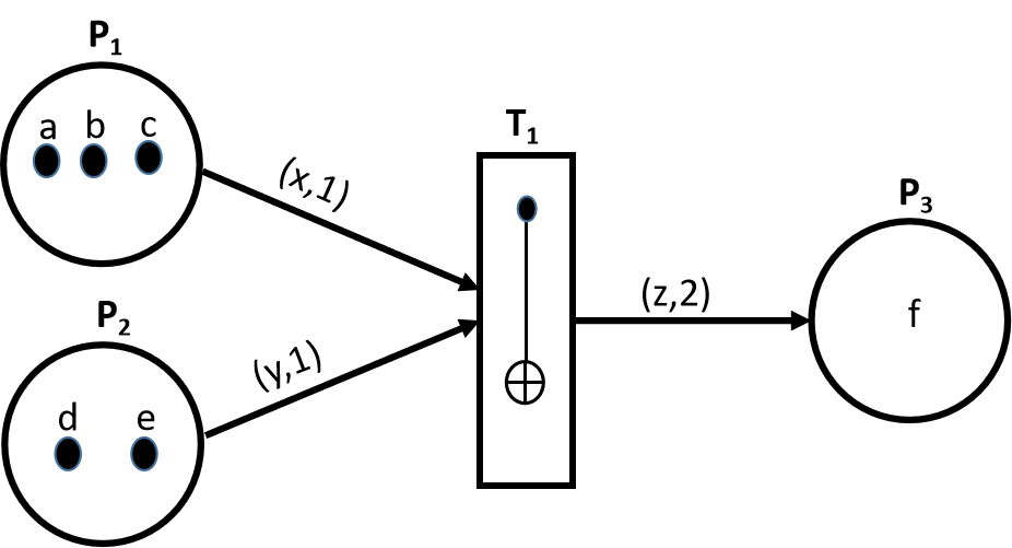
The -tokens in quantum Petri nets represent a set of quantum bits (qubits) or multi-qubits. Qubits are the basic units of quantum information. The -tokens are represented by small black-filled circles in QPN diagrams as shown in Figure 1, where they are identified by letters Places are locations, where -tokens reside. They are represented by the large empty circles in the figure. Each place may hold a certain number of -tokens, and the state of a place is determined by the -tokens it contains. Places and -tokens collectively represent the state of a QPN. Transitions represent quantum events (operations) that can change the state of a QPN, and manipulate -tokens using quantum gates [27]. Directed arcs in link places and transitions together. The direction of an arc determines the flow of -tokens. An arc from a place to a transition indicates that tokens in that place can be consumed by that transition when it fires. An arc from a transition to a place indicates that tokens can be added to that place when the transition fires. The labels on the incoming arcs to a transition such as and denote variables for -tokens that are fed into a transition in the indicated quantities as seen in Figure 1. Similarly the labels on the outgoing arcs from a transition such as denote variables for -tokens that are added into a place in the indicated quantities. For example, one -token in each of places and ( and ) are used by transition in Figure 1, which in this case is a controlled-not (C-NOT) gate. It is assumed that -tokens are consumed by transitions in some predetermined order. In the examples presented here, an alphabetical order will be used to name tokens unless otherwise stated. When fired, a transition manipulates one or more -tokens according to the function that is specified, and moves the generated -tokens to the output places that are connected to that transition. For example, in Figure 1, is placed in i.e., becomes after fires. Transitions in a QPN may represent quantum gates, measurements, or other quantum operations.
 |
Fired transitions are the only means by which -tokens (qubits) move along the arcs. In quantum computing context, these transitions of -tokens in a QPN represent the transformation of quantum states and how they evolve due to quantum parallelism. Effectively, extending the classical Petri net model to a quantum Petri net model adds another layer of control over quantum circuits, one in which quantum operations can be made conditional on the quantities of -tokens.
A marking in a QPN defines the distribution of tokens across the places that represent various configurations or states of the quantum system. The initial state of a QPN is specified by its marking that assigns -tokens to its places. The evolution of the system is then represented by a sequence of changes in the states of the places, driven by the firing of transitions. As transitions fire and tokens move, they alter the overall quantum state of the system. The function represents an assignment of qubits to -tokens under the marking at time in place . Subsequent changes evolve with every transition executed, resulting in
Example:
As can be seen in Figure 1, places , , and have -tokens assigned to them under the following map where and . For this QPN to operate we initialize -tokens to qubits as follows:
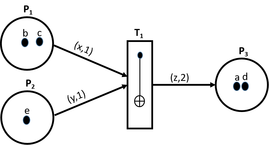
With these assignments, transition will fire at and the places , , and will have the following -tokens at where inverts qubit to
The new state of the QPN is depicted in Figure 2. In the rest of the paper, we will employ the QPN model to design four different quantum buffers.
 |
3 Quantum Buffers
For the purposes of this paper, a quantum buffer is a quantum system in which collections of qubits are structured into quantum packets, which are moved from a set of inputs to a set of outputs. Unlike classical buffers that store and process collections of bits (0’s and 1’s), quantum buffers must obey the properties of superposition, entanglement and coherence of quantum systems. The physical designs of quantum memories using various physical models have been described in [28]. Here, we focus on the conceptual design of quantum buffers using a primitive building block, called a quantum S-R (Q-S-R) flip-flop. The Q-S-R flip-flop is similar to an S-R flip-flop except that it stores a qubit rather than a bit.
 |
| S | R | Q | Q′ | Q-Output |
|---|---|---|---|---|
| Undefined | ||||
| Undefined |
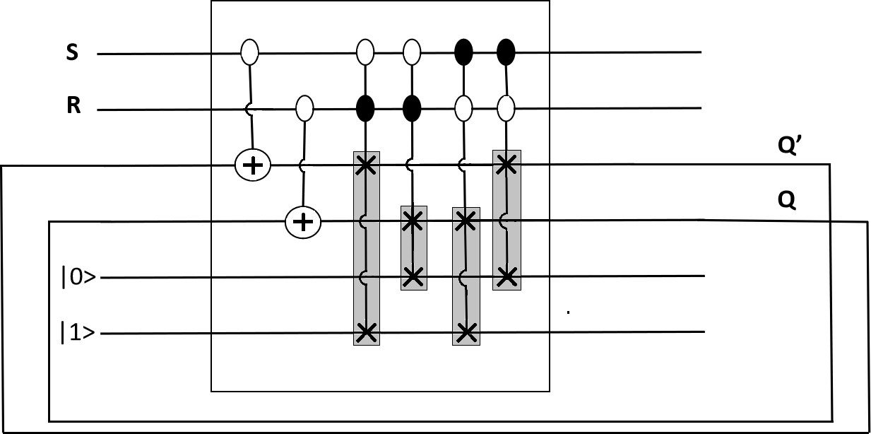
A possible design of a Q-S-R flip-flop is depicted in Figure 3, where and are used as ancillary qubits to clear and set the output. This quantum S-R flip-flop has been designed using two C-NOT and four controlled quantum swap gates with two control inputs and The first two controlled swap gates swap their inputs when and whereas the last two controlled swap gates swap their inputs when and The behavior of the Q-S-R flip-flop is described in Table 1. It can be verified by tracing the qubits from the inputs to the outputs of the diagram in Figure 3. The Q-S-R flip-flops can be put together to obtain quantum registers of any desirable size as in the design of classical registers. For example, a -qubit register can be put together using Q-S-R flip-flops as shown in Figure 4.
Quantum registers are building blocks of quantum buffers that store and process collections of qubits
 |
using quantum gates and circuits. The QPN model that is introduced in the earlier section facilitates this quantum processing, where quantum registers correspond to the places in the QPN model. Places can hold data -tokens (multi-qubits) or ancillary -tokens (multi-qubits). The ancillary -tokens may represent single qubits in some buffer designs and multi-qubits in other buffer designs. They are used used to limit the capacity of a quantum buffer or select a particular transition to fire. By convention, when they represent single qubits, they will arbitrarily be initialized to qubit. The places that exclusively hold data -tokens will be denoted by those that exclusively hold ancillary -tokens will be denoted by and those that hold both data ancillary -tokens will be denoted by with appropriate indexing, such as etc. The places from which -tokens are fed into and taken out of the buffer will be denoted by and respectively with appropriate indexing as well.
3.1 Single Input/Single Output Quantum Buffer
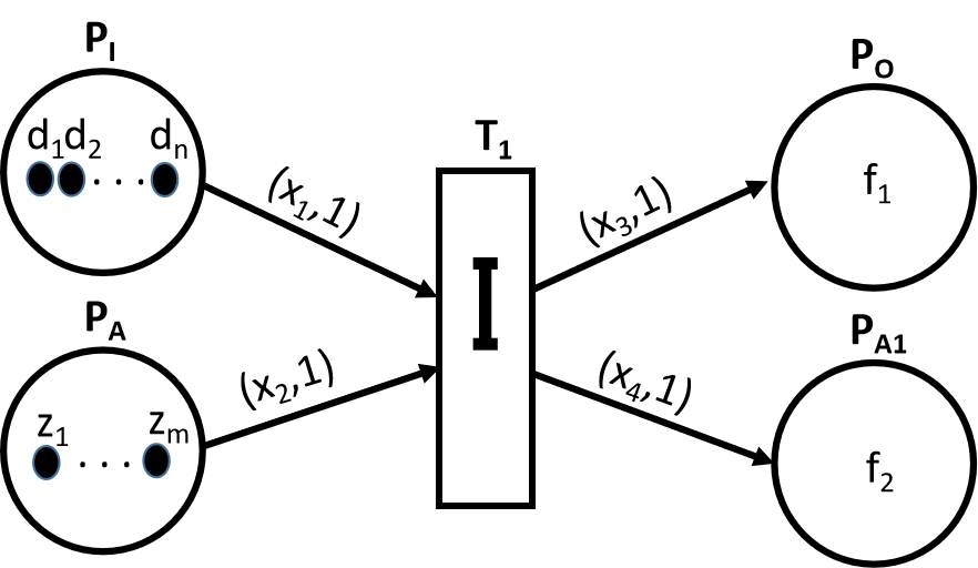
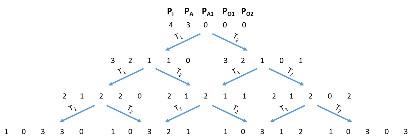
An SISO (Single Input, Single Output) quantum buffer is a type of quantum buffer that has only one entry and one exit point for data -tokens. The SISO buffer is designed to transfer up to -tokens from an input place of data -tokens to an output place that can hold up to -tokens, where it is assumed that The transfer of data -tokens stops when the last ancillary qubit in is consumed by The QPN model of the SISO is thus designed to have a capacity and it consists of a single transition, , four places , data -tokens and ancillary -bits all of which are initialized to qubit. The transition is the identity quantum gate, denoted by , that moves the -tokens in to and the qubits in to The data -tokens are placed in and ancillary qubits are placed in before the buffer starts operating as follows:
 |
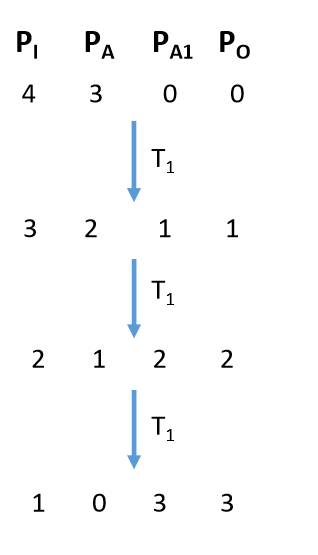 |
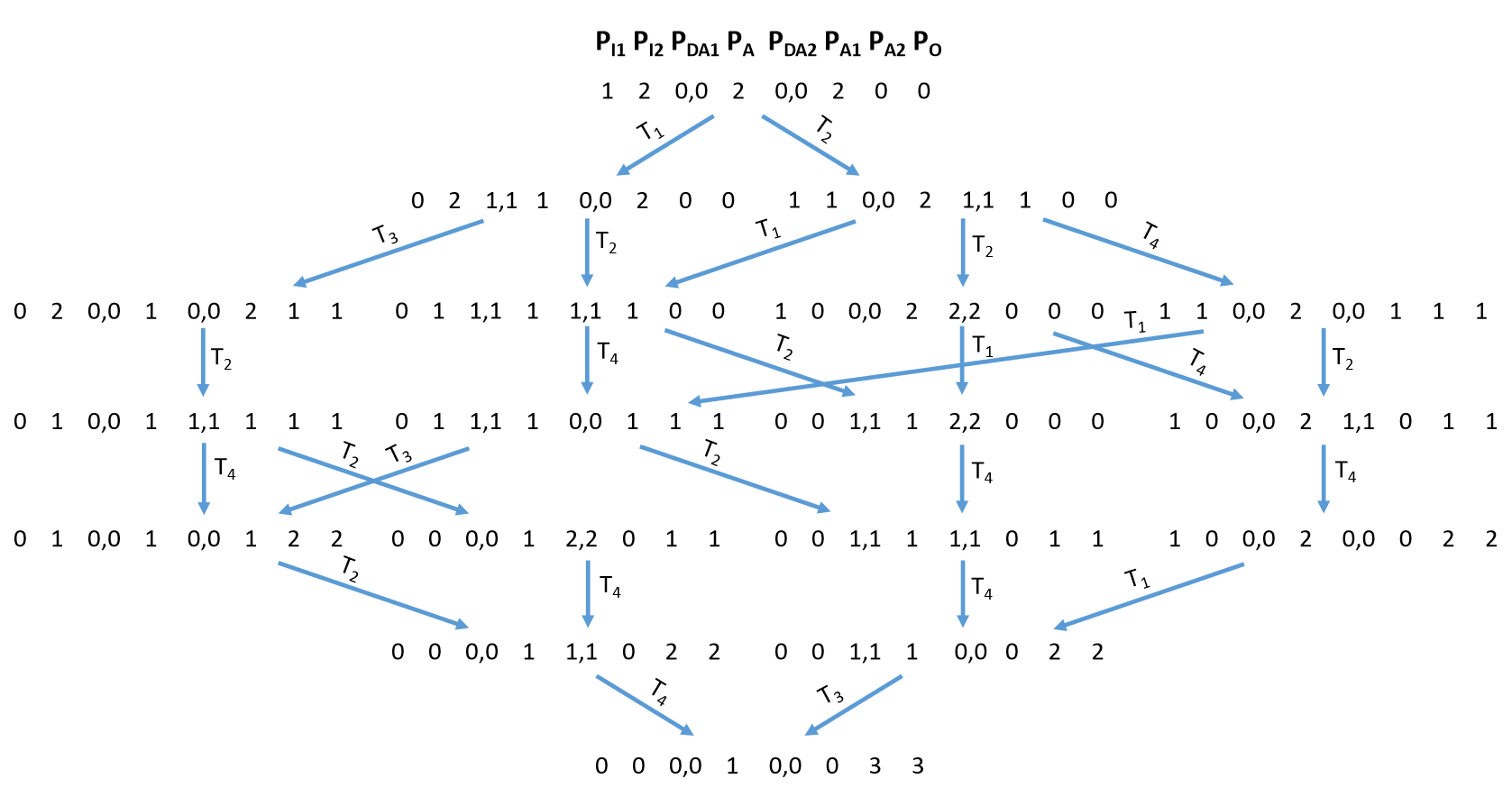
Here, the variables with superscript denote the qubits or multi qubits that are assigned to the data -tokens, at time When the input transition fires, it forwards the current data -token and ancillary qubit, say and to places and respectively i.e., becomes and becomes . The behavior of the SISO buffer of capacity is illustrated in Figure 6. The values that are listed underneath the place labels denote the number of -tokens that are currently located in corresponding places. As seen at the top of Figure 6, initially hold 4, 3, 0, and 0 -tokens, and the number of -tokens in each place changes as the transitions continue to fire. The quantities of -tokens at the end of each transition can be verified by tracing the -tokens as they move between places. To process data -tokens, steps (transitions) are required and the whole process is reversible, and can be repeated again.
3.2 Multiple Input/Single Output Quantum Buffer
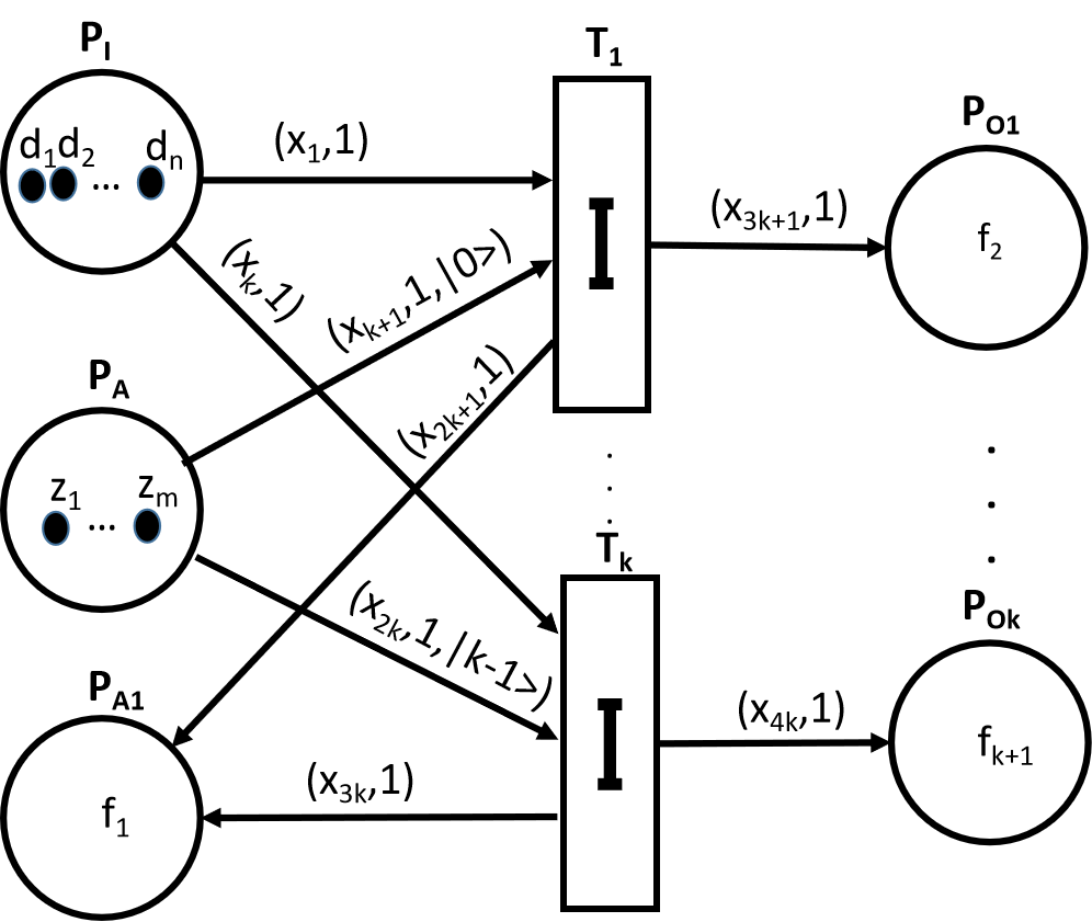
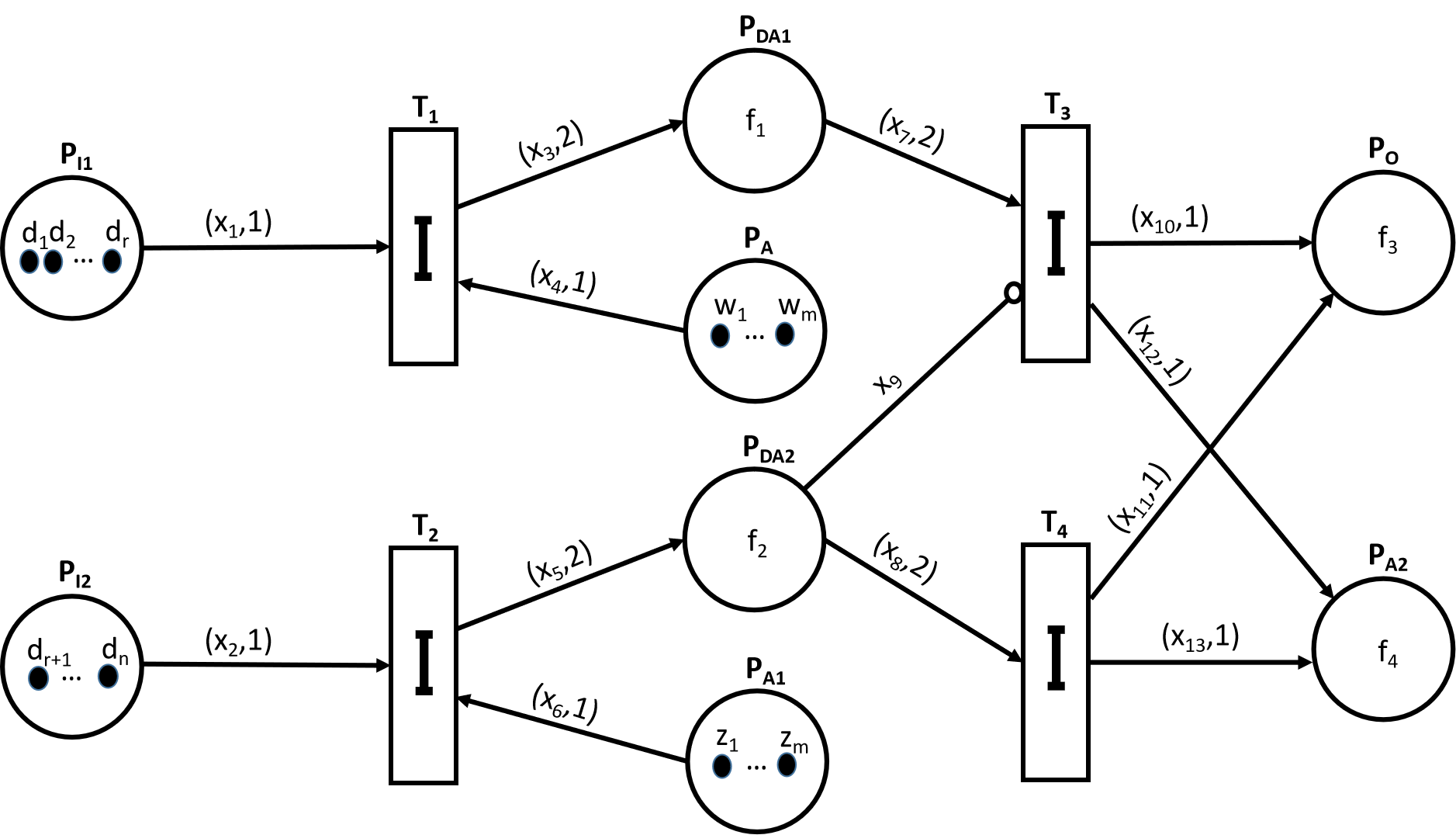
A MISO (Multiple Input, Single Output) quantum buffer is a type of quantum buffer that has many entries and only one exit point for data -tokens. The MISO quantum buffer allows pairing any of its data inputs (places) with its only output place to transfer a -token from that input to the output. Figure 7 depicts the QPN model of MISO quantum buffer with capacity transitions , places , data -tokens in and ancillary -tokens . Each is specified as an address -token that is used to select one of the transitions to fire in order to transfer a data -token in one of the input places to output place via place Each of causes one transition to fire and the MISO buffer halts its operation when all address -tokens are utilized. The labels on the directed arcs denote the variables that represent data -tokens or pairs of data and address -tokens on the incoming and outgoing arcs of transitions. The qubits on the outgoing arcs from denote the address -tokens that serve as selectors of transitions to which the outgoing arcs connect place We note that only one transition fires at a time so that receives two -tokens (one data and one address -token) at any point in time. The -tokens are assigned to places and are initialized before the buffer starts operating as follows:
 |
When the input transition fires it forwards the current data and ancillary -token, say and to place i.e., becomes . When the output transition fires, it forwards the current data and ancillary -token to and respectively. The behavior of the MISO quantum buffer of capacity with two input places and is illustrated in Figure 8. The transitions are fired according to the address values of the ancillary qubits and the number of -tokens in the input places. For example, transition can fire twice along a given sequence of transitions since and place contains two -tokens. On the other hand, transition can only fire once as place has only one -token. The quantities of -tokens at the end of each transition can be verified by tracing the -tokens as they move between places. Some transitions cannot be fired due to -token constraints. To process data -tokens, steps (transitions) are required, the whole process is reversible, and can be repeated again.
 |
3.3 Single Input/Multiple Output Quantum Buffer
A SIMO (Single Input, Multiple Output) quantum buffer is a type of quantum buffer that has only one entry and many exit points for data -tokens. It should be pointed out that the data -tokens in input places are not copied to multiple output places all at once, but each data -token is forwarded to a selected output, one at a time. during each transition can hold up to pairs of data and ancillary -tokens. Figure 9 depicts the QPN model of SIMO quantum buffer of capacity composed of transitions , places , data -tokens and ancillary -tokens each of which can be assigned a quantum value from to . The labels on the directed arcs denote the variables that represent -tokens on the incoming and outgoing arcs of transitions.
 |
The initial -tokens are assigned to places and as in SISO quantum buffer. When transition fires, it forwards the current data and address -tokens to and respectively. The behavior of the SIMO buffer of capacity with two output places and is illustrated in Figure 10.
 |
The quantities of -tokens at the end of each transition can be verified by tracing the -tokens as they move between places. We note that at the end of possible transitions, the four data -tokens may be distributed to and in one of four ways: (3,0), (2,1), (1,2), (0,3) as the bottom row in Figure 10 shows. Also, the value of limits the number of transitions to 3 in this example, preventing transitions with output patterns (4,0) (3,1), (2,2), (1,3), (0,4). The diagram shows only the feasible sequences of transitions, and to process data -tokens, steps (transitions) are needed, where the whole process is reversible, and can be repeated again.
3.4 Multiple Input Multiple Output Quantum Buffer
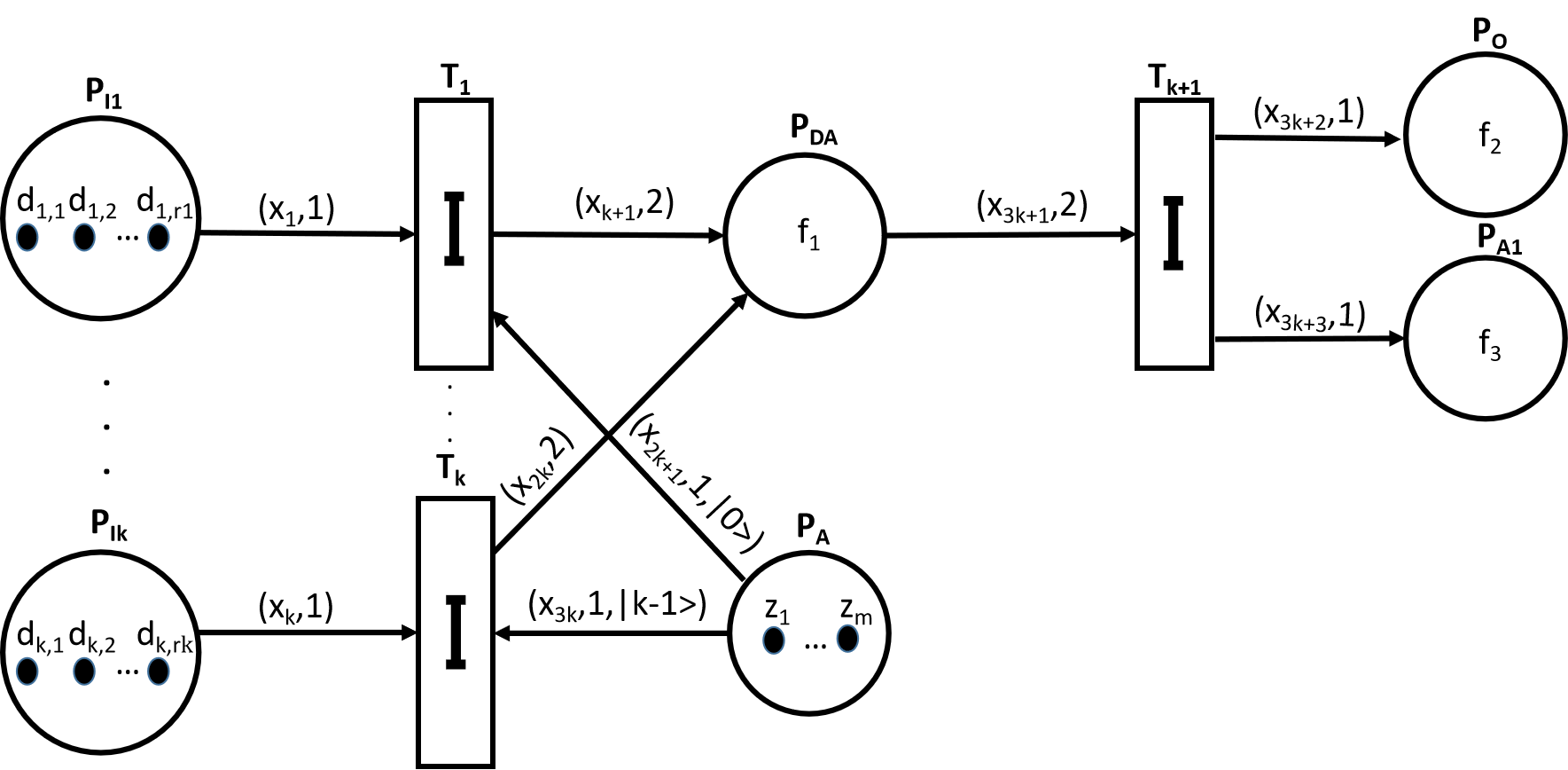
A MIMO (Multiple Input, Multiple Output) quantum buffer is a type of quantum buffer that has multiple entry and multiple exit points for data -tokens. Two sets of ancillary -tokens are used to select the input and output places as the source and destination of a pair of transitions. The ancillary -tokens are used to select an input place, and ancillary -tokens are used to select an output place. Figure 11 depicts the QPN model of MIMO quantum buffer of capacity composed of transitions , input places output places , two ancillary places one joint data/ancillary place data -tokens and ancillary -tokens .
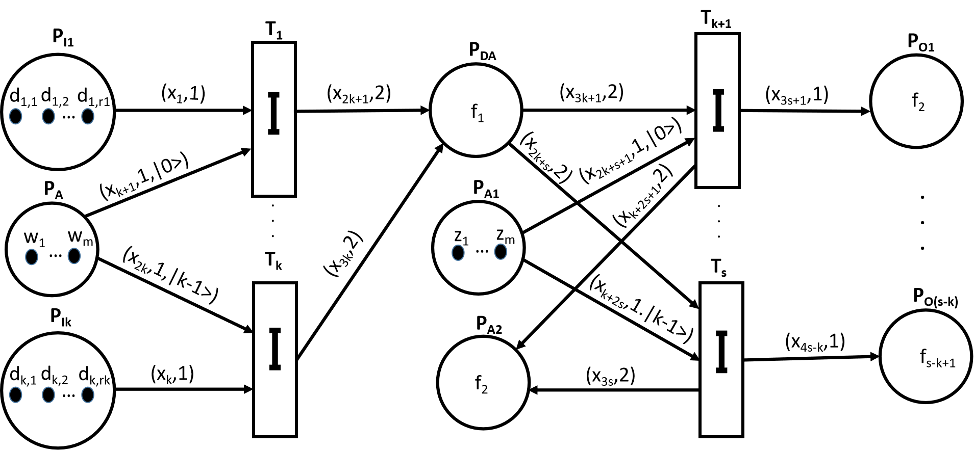 |
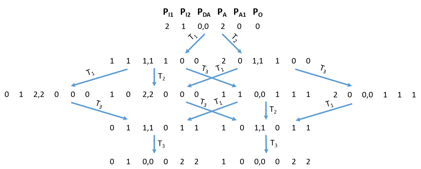
The labels on the directed arcs denote the variables that represent -tokens on the incoming and outgoing arcs of transitions. The data -tokens are assigned to places and as in MISO quantum buffer, and not repeated here. When the input transition fires, it forwards the current data and ancillary -token, say and to place i.e., becomes . When the output transition fires, it forwards an ancillary -token and an ancillary -token to and data -token to the corresponding output place . The behavior of the MIMO quantum buffer of capacity with two input and two output places and is illustrated in Figure 12. Input places and are initialized to two and one -tokens, respectively.
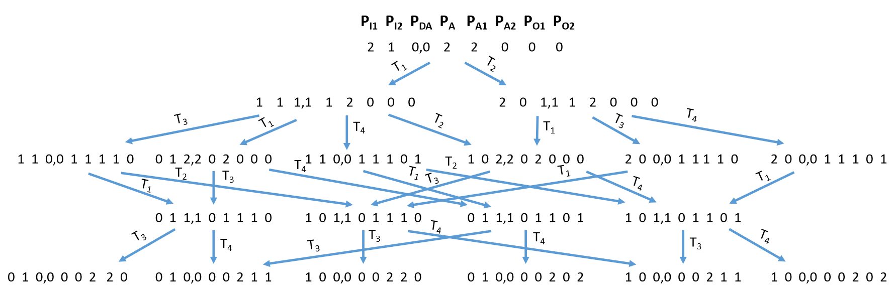 |
The quantities of -tokens at the end of each transition can be verified by tracing the -tokens as they move between places. We note that at the end of possible transitions, the two -tokens may be distributed from input places to output places and in one of six ways: (0,1,2,0), (0,1,1,1), (0,1,0,2), (1,0,2,0), (1,0,1,1), (1,0,0,2) as the diagram in Figure 12 shows. Note that some transition sequences result in identical patterns of -tokens in output places and are counted once. For example, both and result in the placement of one token in each of and It takes transitions, to process data -tokens. Overall, the whole process is reversible, and can be repeated again.
3.5 Priority Quantum Buffer
A priority quantum buffer is a type of quantum buffer that prioritizes the processing of some -tokens over others. Both data and ancillary -tokens are divided into two groups: high priority and low priority. The high priority ancillary -tokens are employed to manage the prioritization of data -tokens that reside in over the data -tokens in during processing. It should be pointed out that the input transitions can run independently. Figure 13 depicts the QPN model of priority quantum buffer with capacity four transitions , eight places , low priority data -tokens, , high priority data -tokens , low priority ancillary -tokens (qubits), and high priority ancillary -tokens (qubits), . The labels on the directed arcs denote the variables that represent -tokens on the incoming and outgoing arcs of transitions. The directed arc also known as inhibitor arc, prevents the firing of output transition if there is any -token present in . The -tokens are assigned to places and and are initialized before the buffer starts operating as follows:
 |
 |
When the input transition, say fires, it forwards the current data and ancillary -token, say and (or ) to place i.e., becomes either (or ). When the output transition, say fires, it forwards the corresponding ancillary -token or to and data -token to . However, the data -tokens in place are prioritized over all tokens in place at the output place because transition cannot fire, due to the constraint of the inhibitor arc . The behavior of the priority quantum buffer of capacity is illustrated in Figure 14. Input places and are initialized to one and two -tokens, respectively. The quantities of -tokens at the end of each transition can be verified by tracing the -tokens as they move between places. We note that some transition sequences inhibit the firing of transition . For example, when fires, it inhibit the firing of transition unless fired. It takes transitions, to process data -tokens. Overall, the whole process is reversible, and can be repeated again.
4 Quantum Buffer Examples
In this section we test the QPN buffer model by implementing the Quantum SR flip-flop and SISO, SIMO, MISO, MIMO and priority quantum buffer designs on the IBM composer [29] and Jupyter [30] using Python and Qiskit [31].
A. Quantum S-R Flip-Flop Runs
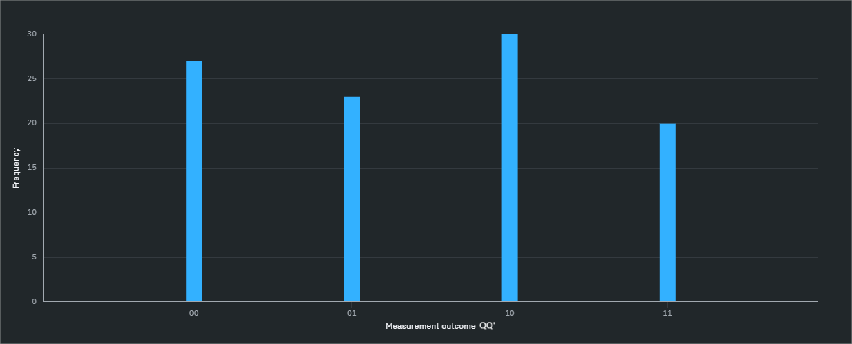
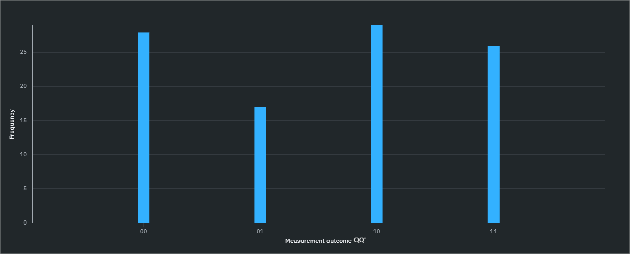
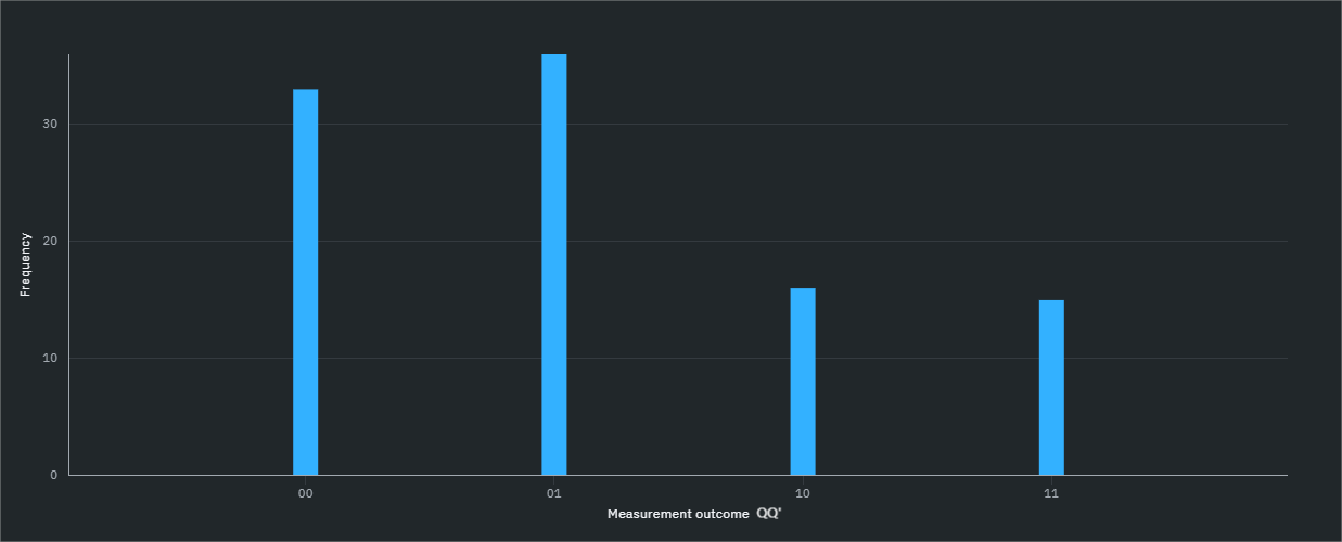
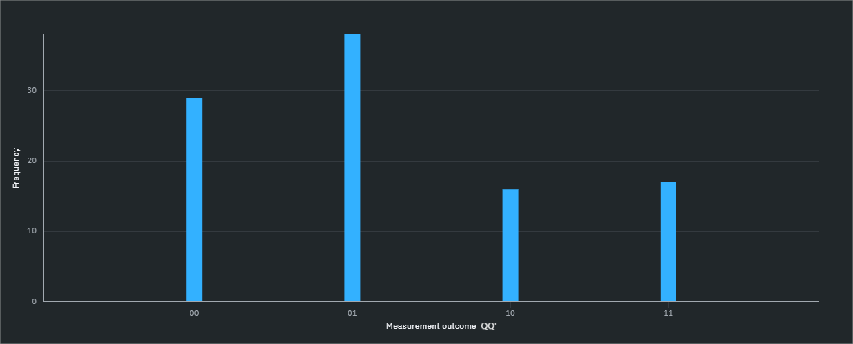
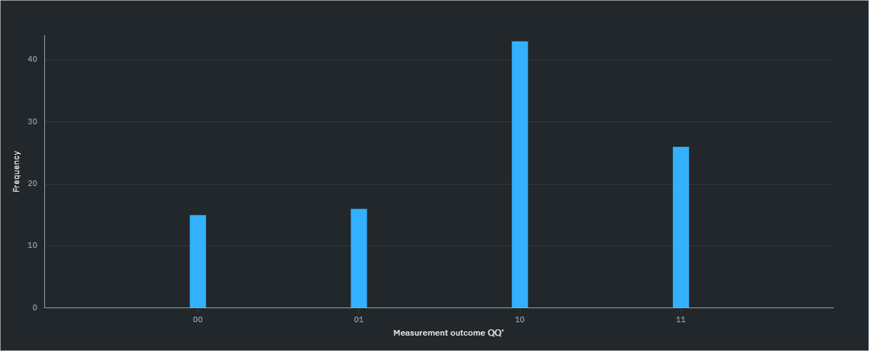
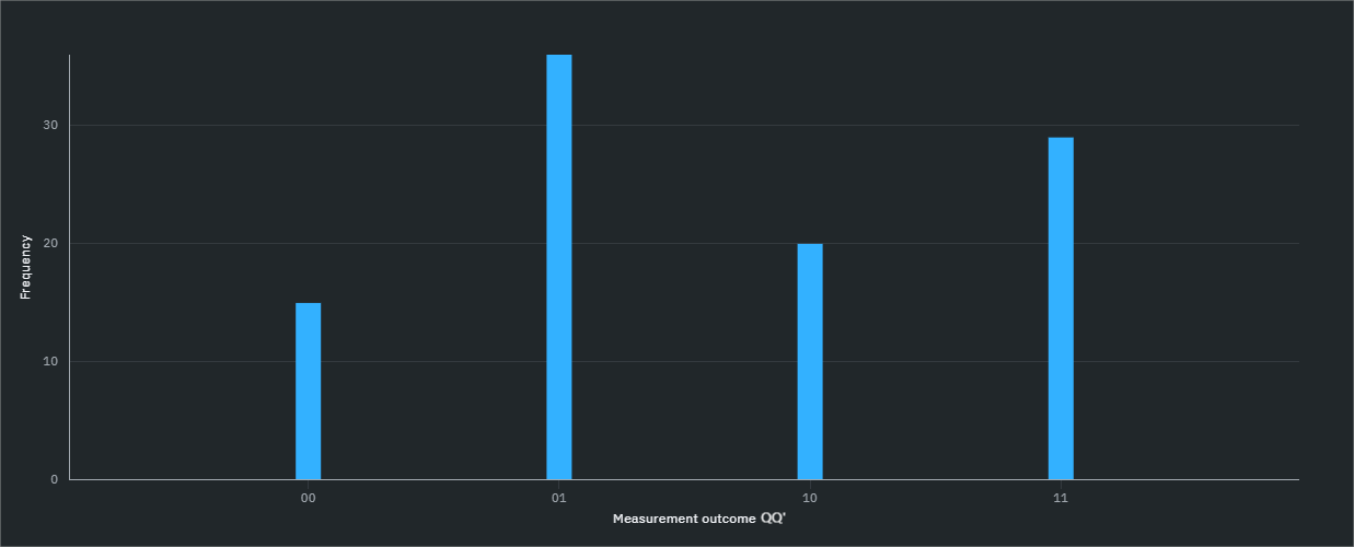
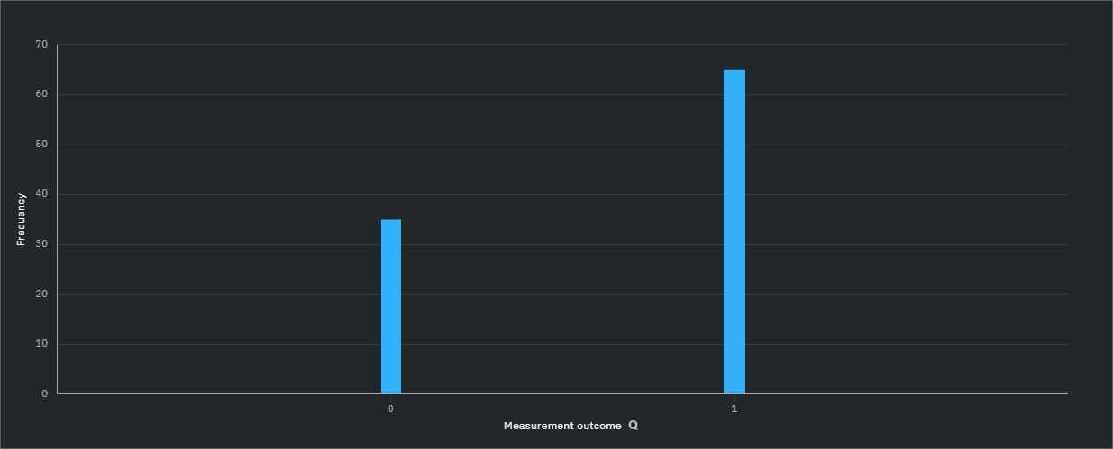
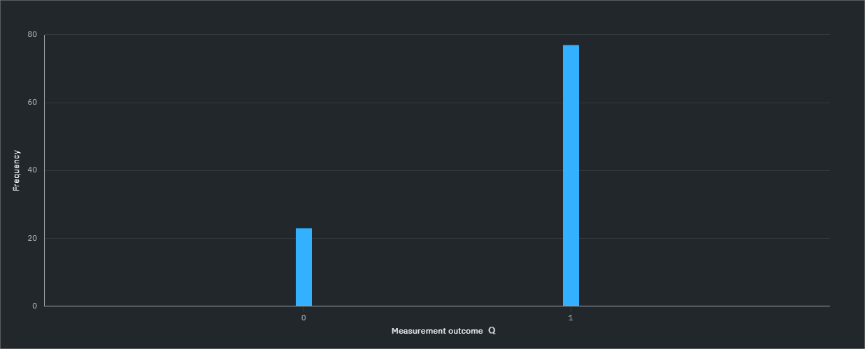
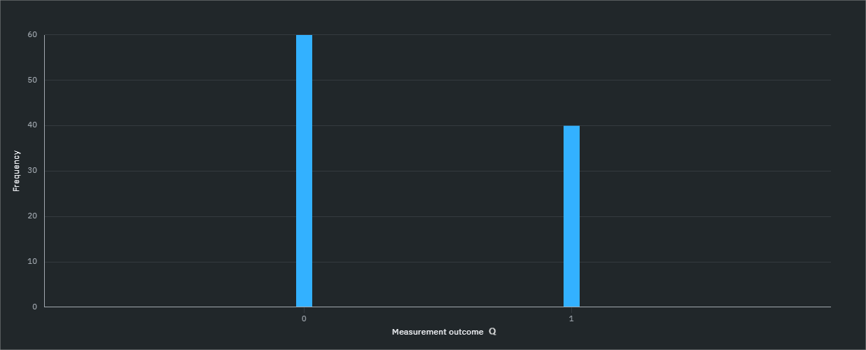
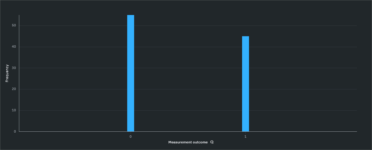
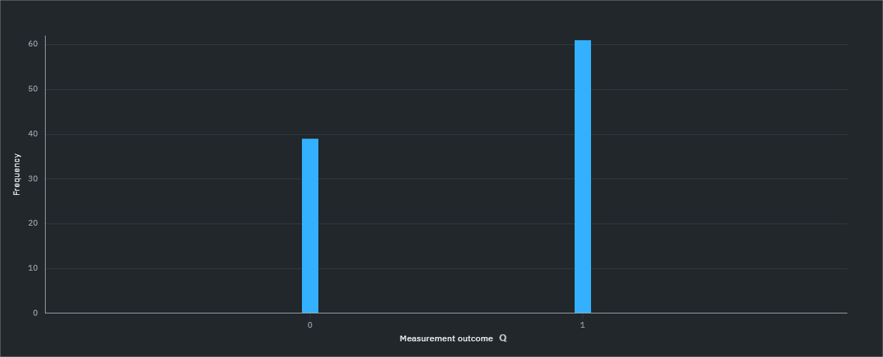
We tested the design of Q-S-R flip-flop in Section 3 on IBM quantum computers under three different settings, i.e., , and when the -state is one of only two valid present states, i.e., and As in a classical S-R flip-flop, the input combination is not allowed for the Q-S-R flip-flop. We performed these runs by measuring both and as well as by measuring either or as depicted in Figure 15 and 16. Both runs were repeated 100 times for each test case. In two qubit measurements in Figure 15, the bars represent the frequencies of from left to right. For the set input, i.e., the Q-S-R flip-flop’s next state, was measured 30 and 29 times, respectively in the present states and both more frequently than the other three states as shown in Figure 15(a) and 15(b). For the reset input, i.e., the next state was measured and times, respectively in the present states and again more frequently than the other states as shown in Figure 15(c) and 15(d). When is set to , the next state was measured and and times, respectively in the present states and as shown in Figure 15(e) and 15(f). Similarly in one qubit measurement in Figure 16, we note that, for the set input, i.e., the Q-S-R flip-flop’s next state, was measured and times, respectively in the present states and as shown in Figure 16(a) and 16(b). For the reset input, i.e., the next state was measured and times, respectively in the present states and as shown in Figure 16(c) and 16(d). When is set to , the next state was measured times, and was measured times, respectively in the present states and as shown in Figure 16(e) and 16(f). These measurements suggest that reading both and leads to more measurement errors than reading only

B. SISO QPN Simulations
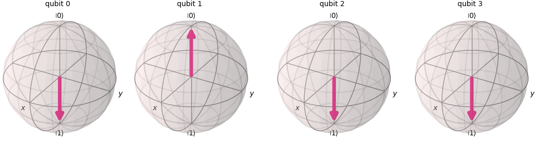
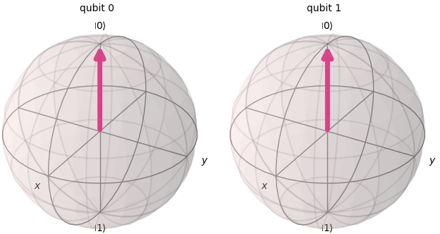
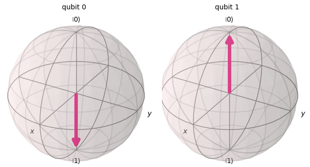
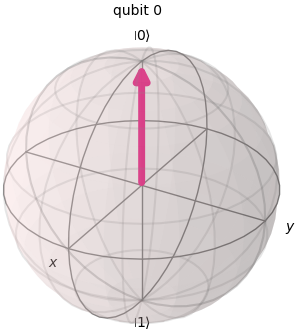
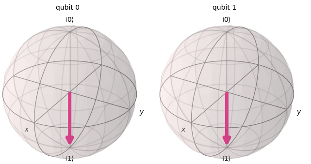
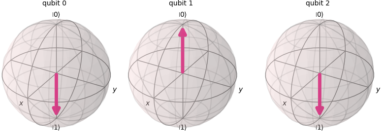
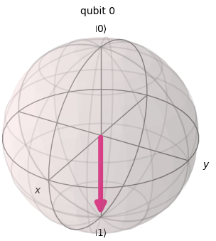
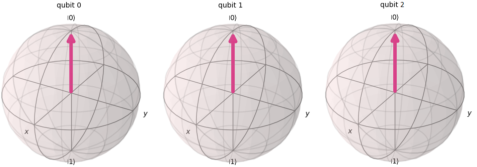
We implement the SISO quantum buffer that was described in Figure 5 with three data -tokens () in and two ancillary -tokens () in where and as shown in Figure 17(a) and 17(b). Initially is enabled and when its fires, it forwards the data -token to and ancillary -token to as shown in Figure 17(c) and Figure 17(d). Again, is enabled and when its fires, it forwards the data -token to and ancillary -token to as shown in Figure 17(g) and 17(i). The data -token will remain in as there is no ancillary -token left in to fire as shown in Figure 17(h). We note that to process two data -tokens, two transitions are fired.
C. SIMO QPN Simulations
We implement the SIMO quantum buffer that was described in Figure 9 with two output places , two transitions , four data -tokens () in and three ancillary -tokens () in where and as shown in Figure 18 (a) and 18 (b). Initially, the first ancillary -token , which enables the transition and when its fires, it forwards the data and ancillary -token and to and . The next ancillary -token , which enables the transition and when its fires, it forwards the data and ancillary -token and to and . Lastly, the ancillary -token enables the transition and when its fires, it forwards the data and ancillary -token and to and as shown in Figure 18(c) and 18(f), whereas data -token will remain in as there is no ancillary -token left in as shown in Figure 18(e).
D. Priority QPN
We implement the priority quantum buffer that was described in Figure 13 with three data -tokens () and four ancillary -tokens () where and . The data and ancillary -tokens and are placed in low priority group and as shown in Figure 19 (a) and 19 (b), whereas data and ancillary -tokens and are placed in high priority group and as shown in Figure 19(c) and 19(d). Initially, the enabled transitions are and , where will fire once and will fire twice, when fires, it forwards the data and ancillary -token and to , when fires, it forwards the data and ancillary -token and to . If is empty, then will fire, otherwise fires. When fires, it forwards the data -token to and ancillary -token to , and when fires, it forwards the data -token to and ancillary -token to as shown in Figure 19(e) and 19 (g), whereas ancillary -token will remain in as there is no data -token left in as shown in Figure 19(f).

5 Concluding Remarks
This paper simplified the quantum Petri net (QPN) model given in [24] and used it to introduce quantum buffer designs to route quantum tokens between a set of input places and a set of output places. It presented a quantum S-R flip-flop that can be used to obtain quantum registers in order to hold quantum tokens at the input and output places and the places within the proposed quantum Petri net buffer designs. Ancillary -tokens have been used in all five designs to fire transitions in order to route data -tokens to their target (output) places. In particular, ancillary -tokens were used as addresses either to select data -tokens from the input places (MISO quantum buffer) or target output places to transfer -tokens (SIMO quantum buffer) or both (MIMO quantum buffer). The design of the quantum S-R-flip-flop was validated using the IBM composer and running the composed quantum circuit on one of IBM’s quantum computers. The quantum buffer designs have been validated using Qiskit and Python. It is noted that, in the MIMO quantum buffer design, the placement of ancillary -tokens into separate places forces a serialization of the transfer of data -tokens from input places to output places. This is done for the clarity of presentation of the MIMO quantum buffer design. The serialization can easily be removed by integrating the ancillary -tokens to the data -tokens within the input places, in which case data tokens can be transferred from input places to output places in parallel according to any assignment between the input and output places. It should be added that a SISO quantum buffer can used to obtain FIFO, LIFO, and any other buffer with a single input place, single output place and a desired ordering of transfers of data -tokens from the input place to the output place by replacing the ancillary qubits by -tokens by the indicies of the data -tokens in the input place. As for future work, it will be worthwhile to validate our quantum buffer designs on an actual quantum computer rather than by Qiskit simulations only. Another direction of research will be to extend the quantum Petri net buffer designs presented here to Petri net versions of multistage quantum packet switching networks[32, 33]. The exploration of these ideas will be deferred to another place.
References
- [1] M. Lanzagorta and Jeffrey Uhlmann. Quantum computer science. Springer Nature, 2022.
- [2] B. I. Djordjevic, Quantum information processing, quantum computing, and quantum error correction: An engineering approach. Academic Press, 2021.
- [3] V. Hassija, et al. Present landscape of quantum computing. IET Quantum Communication 1, No. 2, pp. 42-48, 2020.
- [4] M. Horowitz, E. Grumbling, National Academies of Sciences, Engineering, and Medicine, et al. Quantum computing: progress and prospects. 2019. The National Academies Press.
- [5] W. Scherer. Mathematics of quantum computing. Vol. 11. Springer International Publishing, 2019.
- [6] P. W. Shor. Algorithms for quantum computation: discrete logarithms and factoring. In Proceedings of 35th annual IEEE symposium on foundations of computer science, pp. 124–134, 1994.
- [7] L. K. Grover. A fast quantum mechanical algorithm for database search. In Proceedings of the twenty-eighth annual ACM symposium on Theory of computing, pp. 212-219. 1996.
- [8] A-Y, Rhonda, N. Chancellor, and P. Halffmann. NP-hard but no longer hard to solve? Using quantum computing to tackle optimization problems. Frontiers in Quantum Science and Technology 2, 2023.
- [9] J. Preskill. Quantum computing 40 years later. In Feynman Lectures on Computation, pp. 193-244. CRC Press, 2023.
- [10] T. S. Humble, A. McCaskey, D. I. Lyakh, M. Gowrishankar, A. Frisch, and T. Monz. Quantum computers for high-performance computing. IEEE Micro, 41(5), pp.15–23, 2021.
- [11] D. Bacon and W. Van Dam. Recent progress in quantum algorithms. Communications of the ACM, 53(2): pp. 84–93, 2010. ACM New York, NY, USA.
- [12] S. Ramezani, et.al. Machine learning algorithms in quantum computing: A survey. In 2020 International Joint Conference on Neural Networks (IJCNN), pp. 1-8. IEEE, 2020.
- [13] J-P. Aumasson. The impact of quantum computing on cryptography. Computer Fraud & Security 2017, No. 6. pp. 8-11, 2017.
- [14] P. Danzig, Finite buffers for fast multicast.” ACM SIGMETRICS Performance Evaluation Review 17, No. 1 , pp. 108-117, 1989.
- [15] T. Kimura. Optimal buffer design of an M/G/s queue with finite capacity. Stochastic Models 12, No. 1, pp. 165-180, 1996.
- [16] A. Kougkas, H. Devarajan, and X.-H. Sun. I/O Acceleration via Multi-Tiered Data Buffering and Prefetching. Journal of Computer Science and Technology, 35: pp. 92–120, 2020.
- [17] H. S. Kim and B. S. Ness. Loss probability calculations and asymptotic analysis for finite buffer multiplexers. IEEE/ACM transactions on networking, No. 6, pp. 755-768, 2001.
- [18] J. L. Peterson. Petri nets. ACM Computing Surveys (CSUR), 9(3), pp. 223–252, 1977. New York, NY, USA.
- [19] R. Zurawski and M. Zhou. Petri nets and industrial applications: A tutorial. IEEE Transactions on industrial electronics, 41(6), pp. 567–583, 1994.
- [20] M. Zhou and F. DiCesare. Petri net modeling of buffers in automated manufacturing systems. IEEE Transactions on Systems, Man, and Cybernetics, Part B (Cybernetics), 26(1), pp. 157–164, 1996.
- [21] X. Ye, J. Zhou, and X. Song. On reachability graphs of Petri nets. Computers and Electrical Engineering, 29(2), pp. 263–272, 2003. Elsevier.
- [22] T. S. Letia, E. M. Durla-Pasca, and D. Al-Janabi. Quantum Petri Nets. In 2021 25th International Conference on System Theory, Control and Computing (ICSTCC), pp. 431–436, 2021.
- [23] T. S. Letia, et al. Development of Evolutionary Systems Based on Quantum Petri Nets. Mathematics, 10(23):4404, 2022.
- [24] G. Papavarnavas. Integrating Quantum computing concepts in Petri nets. Bachelor’s Thesis, University Of Cyprus, Department OF Computer Science, 2021.
- [25] K. F. Lee and P. Kumar. Non-Markovian Dynamics in Fiber Delay-line Buffers. arXiv, 2024. DOI: 10.48550/arXiv.2402.00274.
- [26] H. W. Schmidt. How to Bake Quantum into Your Pet Petri Nets and Have Your Net Theory Too. In Service-Oriented Computing: 15th Symposium and Summer School, SummerSOC 2021, Virtual Event, September 13–17, 2021, Proceedings 15, pp. 3-33, 2021.
- [27] J.-L. Brylinski and R. Brylinski. Universal quantum gates. Mathematics of quantum computation, 79, 2002.
- [28] Simon, Christoph, et al. ”Quantum memories: a review based on the European integrated project ’qubit applications (QAP)’.” The European Physical Journal D 58, pp. 1-22, 2010.
- [29] IBM Quantum. IBM Quantum Composer. https://quantum.ibm.com/composer.
- [30] Jupyter, Project Jupyter. https://jupyter.org/.
- [31] IBM Quantum. Qiskit: An Open-source Quantum Computing Framework. Retrieved from https://www.ibm.com/quantum/qiskit.
- [32] M. K. Shukla, , and A. Y. Oruç. Multicasting in quantum switching networks. IEEE Transactions on Computers 59, no. 6, pp. 735-747, 2010.
- [33] R. Ratan and A. Y. Oruç. Self-routing quantum sparse crossbar packet concentrators. IEEE Transactions on Computers 60, no. 10, pp. 1390-1405, 2010.
6 Appendix
Here we list the Open QASM code we used to test the quantum S-R-flip-flop and Qiskit and Python programs to test quantum buffer designs given in the paper.