MSA-3D: dissecting galaxies at with high spatial and spectral resolution
Abstract
Integral field spectroscopy (IFS) is a powerful tool for understanding the formation of galaxies across cosmic history. We present the observing strategy and first results of MSA-3D, a novel JWST program using multi-object spectroscopy in a slit-stepping strategy to produce IFS data cubes. The program observed 43 normal star-forming galaxies at redshifts , corresponding to the epoch when spiral thin-disk galaxies of the modern Hubble sequence are thought to emerge, obtaining kpc-scale maps of rest-frame optical nebular emission lines with spectral resolution . Here we describe the multiplexed slit-stepping method which is times more efficient than the NIRSpec IFS mode for our program. As an example of the data quality, we present a case study of an individual galaxy at (stellar mass , star formation rate yr-1) with prominent face-on spiral structure. We show that the galaxy exhibits a rotationally supported disk with moderate velocity dispersion ( km s-1), a negative radial metallicity gradient ( dex kpc-1), a dust attenuation gradient, and an exponential star formation rate density profile which closely matches the stellar continuum. These properties are characteristic of local spirals, indicating that mature galaxies are in place at . We also describe the customized data reduction and original cube-building software pipelines which we have developed to exploit the powerful slit-stepping technique. Our results demonstrate the ability of JWST slit-stepping to study galaxy populations at intermediate to high redshifts, with data quality similar to current surveys of the universe.
1 Introduction
Galaxies in the nearby universe can be classified according to the “Hubble sequence” of star-forming disks with spiral arms, and passive spheroids (e.g., Hubble, 1926; Kennicutt, 1998). A similar sequence persists at cosmological redshifts of at least (e.g., Wuyts et al., 2011; Mortlock et al., 2013; Zhang et al., 2019; Straatman et al., 2016). Integral field spectroscopy (IFS) has proven critical in understanding the structure of disk galaxies in the early universe, in particular by observing strong emission lines such as H and CO transitions (e.g., see reviews by Glazebrook, 2013; Förster Schreiber & Wuyts, 2020). IFS surveys have revealed that disk galaxies at are characterized by higher velocity dispersion (and lower ratio of rotation to dispersion support, ; e.g., Übler et al. 2019; Leethochawalit et al. 2016; Simons et al. 2016; Epinat et al. 2012; Jones et al. 2021), scale heights characteristic of thick disks (e.g., Elmegreen & Elmegreen, 2006; Hamilton-Campos et al., 2023), shallower gas-phase metallicity gradients (indicating radial mixing; e.g., Wang et al., 2019, 2020), and clumpier star formation morphology (Förster Schreiber et al., 2011; Guo et al., 2015; Livermore et al., 2015), typically lacking the spiral structure seen at low redshifts.
Different factors contributing to the higher gas velocity dispersions at higher redshifts have been proposed theoretically. One effect is that higher gas accretion rates result in higher gas fractions in galaxies, which in equilibrium disk models correlate with higher velocity dispersions (e.g., Dekel et al., 2009; Faucher-Giguère et al., 2013; Brennan et al., 2017; Pillepich et al., 2019; Forbes et al., 2023). Recently, high-resolution cosmological simulations have also found that the thermodynamic state of the circumgalactic medium (CGM) correlates tightly with the emergence of thin disks that can support spiral structure. In particular, Hafen et al. (2022) showed that a virialized inner CGM allows the gas to accrete with coherent angular momentum onto central galaxies via hot-mode accretion, which promotes the formation of thin disks. Stern et al. (2021) also argued that the high and near-uniform thermal pressure in a virialized inner CGM helps confine star formation-driven outflows. In a related study, Hopkins et al. (2023) emphasized the role of the concentration and depth of the gravitational potential. The former is a determinant of whether there is a well-defined dynamical center around which rotation can stabilize, while the latter (which correlates with CGM virialization) contributes to the confinement of outflows via gravity (see Byrne et al., 2023, for a discussion of outflow confinement by hot gas pressure vs. gravity). In this picture in which the emergence of thin disks is connected to the virialization of the inner CGM and the depth of the gravitational potential, mass rather than redshift is a primary predictor of thin-disk formation. In practice, this leads to an increased thin-disk fraction going to lower redshift because the abundance of sufficiently massive halos ( M⊙) increases with decreasing redshift.
Observationally, the epoch around is thought to be a time of “disk settling” during which thin spiral disks become prominent among star forming galaxies (e.g. Kassin et al., 2012; Miller et al., 2011, 2012; Simons et al., 2017).
Surveys of galaxy kinematics indicate a rise in the degree of rotational support revealed by increasing toward lower redshifts (as well as higher at higher masses; e.g., Wisnioski et al., 2019; Simons et al., 2016; Tiley et al., 2021). For example, Simons et al. (2017) show that the fraction of massive galaxies (stellar mass ) with increases from 20% at to approximately 50% at . Morphological studies similarly show an increasing fraction of disk and spiral galaxies at lower redshifts. While clear examples of spiral galaxies have been found as early as (e.g., Wu et al., 2023), they are rare at such redshifts. Recent analysis of James Webb Space Telescope (JWST) imaging by Kuhn et al. (2024) found that the fraction of massive galaxies () with visually identifiable spiral structure increases from 15% at to 43% at , although the true spiral fraction is likely higher given the challenge of detecting spiral structure at high redshifts. Previous investigations of Hubble Space Telescope images found broadly similar results (e.g., Margalef-Bentabol et al., 2022). Overall, morphological and kinematic properties both indicate that well-ordered disks are more common at lower redshift, with the population of moderately massive star-forming galaxies becoming dominated by spiral disk morphologies at around .
High-quality IFS observations of strong nebular emission lines (such as H, [N II], and [O III]) can provide a comprehensive view of individual high-redshift galaxies and their evolutionary pathways. For example, kpc-scale kinematic measurements can reveal the mass density profile and dark matter fraction (e.g., Genzel et al., 2020). In addition to kinematics and morphology, strong emission line ratios provide information about ionization sources (e.g., Wright et al., 2010; Belli et al., 2017) and gas-phase metallicity (e.g., Maiolino & Mannucci, 2019). Radial metallicity gradients have emerged as a valuable probe of the “baryon cycle” of gas accretion and feedback-driven outflows which regulate galaxy formation (Tumlinson et al., 2017; Faucher-Giguère & Oh, 2023), as established by various theoretical investigations (Gibson et al., 2013; Ma et al., 2017; Hemler et al., 2021). Metallicity and kinematic maps can also identify signatures of metal-poor gas accretion (e.g., Sánchez Almeida et al., 2015; Ju et al., 2022). Observations of high-redshift galaxies have found a large scatter in gradient slopes, which are shallower on average than in nearby spiral galaxies and show substantial azimuthal variation (e.g., Wang et al., 2017, 2020, 2022; Curti et al., 2020). As with kinematics, spatial resolution of kpc is essential for accurate results (Yuan et al., 2013; Jones et al., 2013). IFS emission line maps can thus not only identify disks via their kinematic signatures, but also probe the properties such as accretion and gravitational potential, which allow the formation of thin spiral disks.
A key challenge for high redshift galaxies is to obtain IFS with sufficient angular resolution, as well as spectral resolution and signal-to-noise ratio. For the rest-frame optical emission lines, the vast majority of current samples are observed with seeing-limited data of 05–10 resolution. This corresponds to 4–8 kpc at (e.g., Förster Schreiber et al., 2009; Wisnioski et al., 2015, 2019; Stott et al., 2016) which is comparable to massive galaxy sizes at these redshifts. Such data cannot clearly distinguish disks from merging systems at moderate to high redshifts (e.g., Leethochawalit et al., 2016; Simons et al., 2019). Instead, the prevalence and kpc-scale structure of rotationally supported disks at redshifts has been established in smaller samples with adaptive optics (AO) assisted observations (e.g., Genzel et al., 2006, 2008; Förster Schreiber et al., 2018; Espejo Salcedo et al., 2022), including AO surveys of gravitationally lensed galaxies which can probe 100 parsec scales (Stark et al., 2008; Jones et al., 2010; Leethochawalit et al., 2016; Hirtenstein et al., 2019). However, current AO systems are most effective only at wavelengths m. Consequently, most AO IFS samples are limited to where H and other strong lines can be observed with high Strehl ratios. As a result, the epoch of spiral disk emergence at –1.5 has not been explored with suitable resolution. Additionally, ground-based observations suffer from a time-variable atmosphere and point-spread function (PSF), which is especially complex for AO data. This leads to challenges in recovering properties such as galaxy velocity dispersions and (e.g., Davies et al., 2011; Burkert et al., 2016). We note that space-based grism observations are able to obtain kpc-scale spatial resolution but are limited by poor spectral resolution (; e.g., Simons et al., 2021; Wang et al., 2020; Jones et al., 2015b), while ground-based IFS surveys are limited to coarse spatial resolution at the key wavelengths.
JWST’s unique capabilities now enable excellent spatial and spectral resolution, combined with good sensitivity at the relevant wavelengths for mapping rest-frame optical emission lines at with the NIRSpec instrument (Jakobsen et al., 2022; Böker et al., 2023). Importantly, JWST delivers reliable results via a stable PSF with high Strehl, in contrast to ground-based AO observations. However, NIRSpec’s integral field unit (IFU) is effectively limited to single-object observations given the 3″ field of view. Building sufficient samples to characterize the galaxy population at high redshifts is thus a time-intensive prospect. To efficiently obtain high-quality data for large samples, we have instead turned to NIRSpec’s Micro-Shutter Assembly (MSA) which provides multiplexed observations with 02 wide slitlets. By utilizing a “slit-stepping” observing sequence (e.g., Ho et al., 2017; Genzel et al., 2013), we are able to obtain IFS data for 40 galaxies simultaneously in % of the time that would be required for an equivalent IFU survey. This paper describes our first application and example results of this novel multiplexed slit-stepping method via the program JWST-GO-2136, in which we observed 43 galaxies at , corresponding to the disk settling epoch when spiral structure becomes prominent. As we are obtaining 3-D data cubes using NIRSpec’s MSA strategy, we dub our program MSA-3D111With a nod to previous surveys 3D-HST (Brammer et al., 2012) and KMOS3D (Wisnioski et al., 2015)..
In this paper, we demonstrate that our technique provides excellent data quality for mapping galaxies, which our team is analyzing with a series of planned papers on their kinematics, metallicity gradients, excitation sources, star formation morphology, and more. Notably, our sample size obtained with a 30 hour MSA slit-stepping program is comparable to the 47 galaxies targeted by the 273-hour NIRSpec guaranteed time GA-NIFS program using the IFU (Perna, 2023). Given the large efficiency gain over JWST’s IFU mode, our method represents the most pragmatic opportunity to build large samples (tens to hundreds) of kpc-resolution IFS data of distant galaxies to study their evolution across cosmic time. Accordingly, one of our objectives in this paper is to simply demonstrate the effectiveness of this observing strategy. We urge its adoption for large multiplexed galaxy surveys with JWST.
This paper describes the observational strategy and data reduction procedure, serving as a reference for the MSA-3D program and subsequent papers. We also describe a case study of an individual galaxy illustrating the variety of analyses enabled by MSA-3D. Various analyses of the broader sample are in preparation or planned. These include a companion paper by Ju et al. (in prep.) presenting the gas-phase metallicity gradients, a study of the gas ionization mechanisms and active galactic nuclei (Roy et al. in prep.), and other topics such as kinematics, angular momentum, dark matter content, and star formation rate profiles. The structure of the present paper is as follows. In Section 2 we describe the JWST observations, including the sample selection, motivation and implementation of the slit-stepping methodology, and data processing. Section 3 presents a case study of a spiral galaxy based on emission line measurements from our data. We describe its kinematic structure, gas-phase metallicity and radial gradient, dust attenuation and radial gradient, and overall disk structure as traced by the surface brightness profile. In Section 4 we discuss our results, and future analyses enabled by the MSA-3D program, in the context of broad efforts to understand the growth and evolution of galaxies across cosmic history. Throughout this work we adopt a flat CDM cosmology with H km s-1 Mpc-1 and (Bennett et al., 2014).
| ID | RA | Dec | stellar mass | SFR | emission lines | |
|---|---|---|---|---|---|---|
| 2111 | 215.0627824 | 52.9070766 | 0.58 | 9.97 | 1.6 | H, [N II], [S II], [S III] |
| 2145 | 215.0694675 | 52.9108516 | 1.17 | 9.19 | 1.4 | H, [N II], [S II], H, [O III] |
| 2465 | 215.0704381 | 52.9137241 | 1.25 | 9.30 | 1.6 | H, [N II], [S II], H, [O III] |
| 2824 | 215.0685025 | 52.914333 | 0.98 | 9.49 | 0.7 | H, [N II], [S II], [O III], [S III] 9069 |
| 3399 | 215.042511 | 52.8996031 | 1.34 | 9.81 | 3.5 | H, [N II], [S II], H, [O III] |
| 4391 | 215.0676175 | 52.9232437 | 1.08 | 9.48 | 2.7 | H, [N II], H, [O III] |
| 6199 | 215.0450158 | 52.9194652 | 1.59 | 10.00 | 17.8 | H, [N II], [S II], H |
| 6430 | 215.0131444 | 52.8980378 | 1.17 | 9.79 | 8.9 | H, [N II], [S II], H, [O III] 4959 |
| 6848 | 215.0355588 | 52.9166925 | 1.57 | 10.64 | 7.8 | H, [N II], [S II], [O III] |
| 7314 | 214.9989097 | 52.8925151 | 1.28 | 9.55 | 2.6 | H, [N II], H, [O III] |
| 7561 | 215.0609094 | 52.9383828 | 1.03 | 9.21 | 0.7 | H, [N II], [S II], H, [O III], [S III] 9069 |
| 8365 | 215.0599904 | 52.9422373 | 1.68 | 9.56 | 3.4 | H, [N II], [S II], H, [O III] |
| 8512 | 215.0497806 | 52.9380795 | 1.10 | 10.32 | 3.2 | H, [N II], [S II], H, [O III] |
| 8576 | 215.0595679 | 52.9434335 | 1.57 | 9.60 | 3.3 | H, [N II], [S II], H, [O III] |
| 8942 | 215.0094032 | 52.9100655 | 1.18 | 9.86 | 16.2 | H, [N II], [S II], H, [O III] 4959 |
| 9337 | 214.9957065 | 52.9019407 | 1.17 | 9.27 | 2.2 | H, [N II], [S II], H, [O III] |
| 9424 | 214.9926533 | 52.900911 | 0.98 | 9.76 | 5.4 | H, [N II], [S II] |
| 9482 | 215.0530158 | 52.9442406 | 1.21 | 9.77 | 0.7 | H, [N II][S II], H, [O III] |
| 9527 | 215.0085005 | 52.9123786 | 1.42 | 10.02 | 2.8 | H, [N II], H, [O III] |
| 9636 | 215.0365985 | 52.9328783 | 0.74 | 9.35 | 1.7 | H, [N II], [S II], [S III] |
| 9812 | 215.0402843 | 52.9376004 | 0.74 | 9.97 | 3.6 | H, [N II], [S II], [S III] |
| 9960 | 215.031894 | 52.9331513 | 1.51 | 11.06 | 6.0 | H, [N II], [S II] |
| 10107 | 214.9817759 | 52.8975743 | 1.01 | 10.01 | 3.6 | H, [N II], [S II], [O III] |
| 10502 | 214.9857711 | 52.9033048 | 1.23 | 10.13 | 4.7 | H, [N II], H, [O III] |
| 10752 | 215.0403761 | 52.9413773 | 1.73 | 9.62 | 3.9 | H, [O III] |
| 10863 | 215.0551264 | 52.9529908 | 1.03 | 9.24 | 1.1 | H, [N II], H, [O III], [S III] 9069 |
| 10910 | 215.0561932 | 52.9553701 | 0.74 | 9.57 | 1.5 | H, [N II], [S II], [S III] |
| 11225 | 215.0415788 | 52.9454655 | 1.05 | 9.67 | 12.6 | H, [N II], [S II], H, [O III] |
| 11539 | 214.9819651 | 52.9051336 | 1.61 | 10.39 | 6.5 | H, [O III] |
| 11702 | 214.9794086 | 52.9031601 | 1.23 | 9.37 | 1.3 | H, [O III] |
| 11843 | 215.0390468 | 52.9471037 | 1.46 | 10.74 | 19.0 | H, [N II], [S II], H, [O III] |
| 11944 | 215.0369901 | 52.9453937 | 1.04 | 9.27 | 1.0 | H, [N II], [S II], H, [O III] |
| 12015 | 215.0323151 | 52.9431798 | 1.24 | 10.08 | 11.2 | H, [N II], [S II], H, [O III] |
| 12071 | 215.0219665 | 52.9360567 | 1.28 | 9.47 | 1.6 | H, [N II], [S II], H, [O III] |
| 12239 | 215.0495343 | 52.9560252 | 0.89 | 9.49 | 1.5 | H, [N II], [S II], [S III] |
| 12253 | 215.0442096 | 52.9520815 | 1.03 | 9.17 | 2.0 | [S II], H, [O III] |
| 12773 | 215.029765 | 52.9451588 | 0.95 | 9.23 | 1.0 | H, [N II], [S II] |
| 13182 | 214.99983 | 52.9268186 | 1.54 | 10.25 | 15.8 | H, [O III] |
| 13416 | 215.0252815 | 52.9456859 | 1.54 | 10.76 | 20.0 | H, [N II], [S II], [O III] |
| 18188 | 214.9839579 | 52.9413562 | 0.82 | 9.56 | 0.9 | H, [N II], [S II] |
| 18586 | 214.9712282 | 52.9337862 | 0.76 | 9.01 | 3.3 | H, [N II], [S II] |
| 19382 | 214.9765628 | 52.9414977 | 1.03 | 9.38 | 0.6 | H, [N II], [S II], [O III] |
| 29470 | 214.9689505 | 52.9453733 | 1.04 | 9.71 | 2.1 | H, [N II], [S II], H, [O III] |
2 Observations and Data Processing
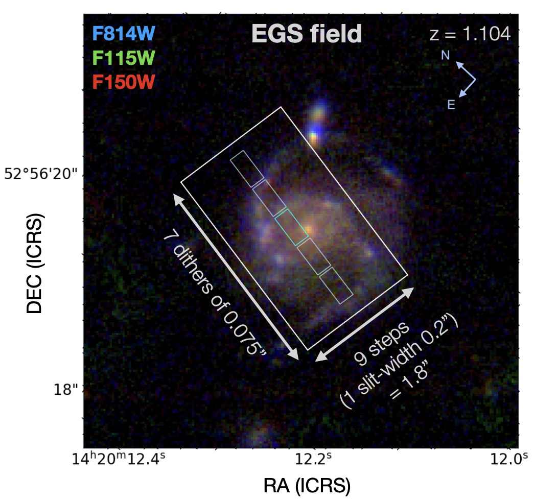
This paper is based on spectroscopic data from the JWST Cycle 1 program GO-2136 (PI: Jones). This program obtained NIRSpec Micro-Shutter Assembly (MSA) observations of 43 galaxies at , using a slit-stepping strategy to provide spatially resolved kpc-scale pseudo-integral field spectroscopy. Data were taken on 2023 March 29-30. We used the G140H/F100LP grating/filter combination, covering wavelengths 0.97–1.82 m with full-width at half maximum (FWHM) spectral resolution Å corresponding to resolving power. As described below, dithered exposures cover a contiguous 18(20–30) field of view for each target galaxy, depending on the number of slitlets used. The observations are optimized to map strong rest-frame optical emission lines in galaxies spanning the epoch in which modern thin disks emerge (e.g. Kassin et al., 2012; Miller et al., 2012; Simons et al., 2017; Wisnioski et al., 2019). In this section, we describe the observing strategy, the merits of the MSA slit-stepping approach relative to the IFU mode, and the data reduction steps performed to produce data cubes.
2.1 Sample selection
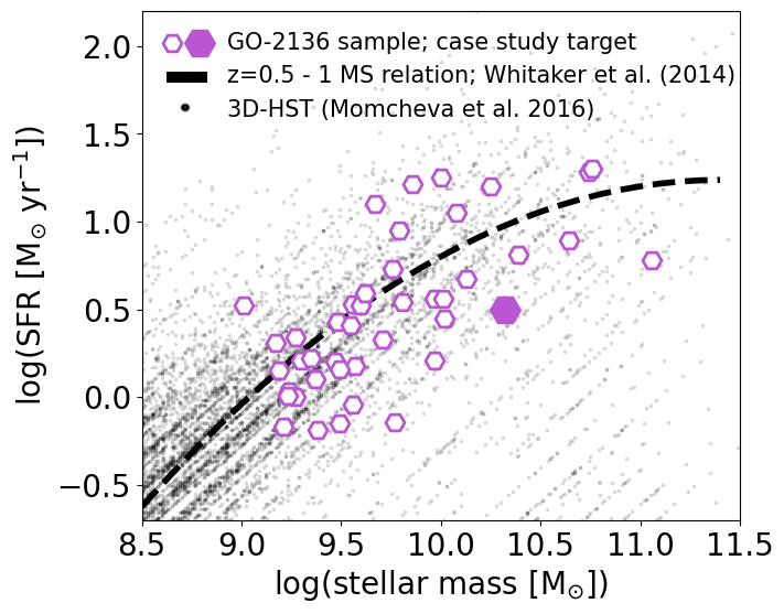
Our target field is the Extended Groth Strip (EGS), a well-studied extragalactic field with extensive photometric and spectroscopic survey data including from the CANDELS (Koekemoer et al., 2011), 3D-HST (Momcheva et al., 2016), CEERS (Finkelstein et al., 2023), DEEP2 and DEEP3 (Newman et al., 2013), and MOSDEF (Kriek et al., 2015) surveys. This field was selected in part to overlap with the CEERS JWST Early Release Science imaging area. Our program science goals require mapping multiple nebular emission lines to study resolved kinematics, star formation rates, metallicity, and ionization mechanisms. Our primary sample selection is to target H, [N II], [S II], [O III], and H. These lines are accessible from –1.7 using the G140H/F100LP grating/filter. We adopt a secondary target redshift range –1.0 which includes coverage of H, [N II], [S II], [S III], and H I Paschen lines, enabling similar measurements. For target selection, we required spectroscopic redshift confirmation and multi-wavelength HST photometry from the CANDELS survey (Koekemoer et al., 2011), which, along with other imaging data, ensures reliable spectral energy distribution fitting based measurements of stellar mass and star formation rate (SFR). For selection purposes, we adopted stellar population parameter values from the 3D-HST survey catalogue (Skelton et al., 2014; Momcheva et al., 2016). In total, we identified a parent catalog of 1336 galaxies in the target redshift range , and further restricted the MSA target selection to the 72% of these galaxies with secure spectroscopic redshifts. The sample is shown in the left panel of Figure 1.
In building our spectroscopic sample, we applied selection criteria of stellar mass and SFR . This ensures the observed targets probe the star forming main sequence at (e.g., Whitaker et al., 2012; Speagle et al., 2014) and have suitably bright and spatially extended nebular emission. However, we did not impose any selection criteria based on galaxy size or surface brightness to avoid biases in the observed sample. In designing the MSA mask, we also targeted regions with JWST/NIRcam coverage from the CEERS program. Ultimately, the MSA mask includes 43 target galaxies, of which 19 are within the current NIRCam footprint. Table 1 lists properties and emission line coverage of these 43 galaxies, of which 32 are at and 11 are at . Coverage of the H line is present in 38 of the 43 galaxies (88%), whereas in the remainder of the sample it falls in the chip gap or off the detectors. In this paper we present a case study analysis of galaxy ID 8512 at with and SFR . We selected this target for initial analysis based on its clear spiral disk morphology. It is otherwise representative of the more massive galaxies in the observed sample.
2.2 Slit-stepping observing strategy
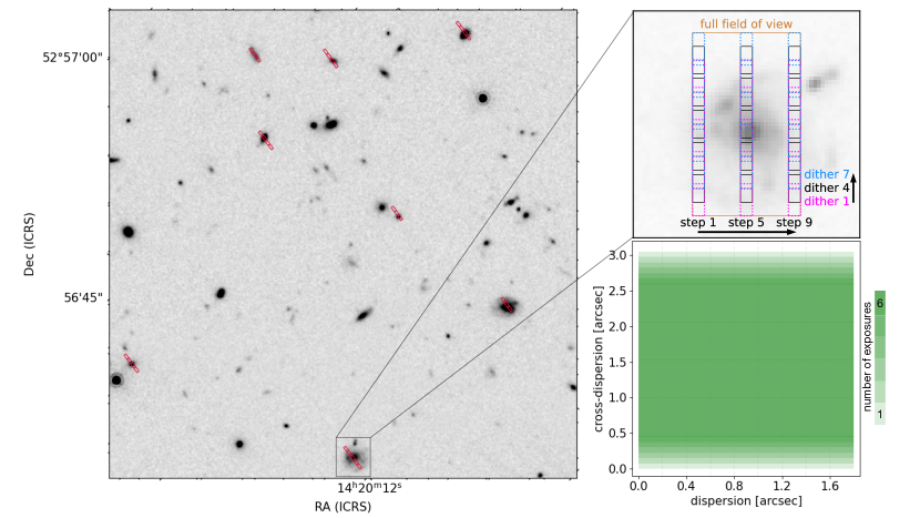
A key unique aspect of these JWST Cycle 1 observations is the slit-stepping strategy illustrated in Figure 2. We observed the same MSA mask configuration in a grid of 63 different pointings: 9 steps along the dispersion direction at a width of a slitlet (02), with 7 dithers along the cross-dispersion direction stepped by the width of a barshadow (0075). A single exposure of 19.5 minutes was taken at each of the 63 dithered positions, using the NRSIRS2 readout mode with 16 groups. This 97 dither pattern provides nearly uniform depth, where each sky position is observed with six exposures on-source (117 minutes) and one exposure affected by a bar shadow. Each target galaxy is covered with a minimum of 3 slitlets of 05 length each. We add up to 2 additional slitlets wherever possible, avoiding MSA slit collisions. This results in data cubes spanning 18(20–30) depending on the number of slitlets (3–5), as illustrated in Figures 1 and 2. The region with uniform full exposure coverage is 18(11–21), corresponding to approximately 15(10-18) kpc at our target redshifts. We emphasize that the slit-stepping strategy is designed for contiguous uniform depth in this field of view. In contrast, a rectangular grid of slitlets (e.g., 95) on the MSA has only 65% illumination with approximately one-third of the area obscured by bar shadows. Our observations effectively remove these bar shadows to provide contiguous sky coverage Figure 2).
The areal coverage set by the number of slit-steps (9) and slitlets per target () is chosen to sample galaxy radii , where kpc is the typical scale radius of star-forming galaxies at the upper mass range of our sample (). A key goal is to map galaxy kinematics beyond the “turnover radius” () corresponding to the maximum circular velocity for an exponential disk (Freeman, 1970). The depth of 2 hours effective exposure time is sufficient to reach detections of H emission in an 0102 resolution element at for typical galaxies across the targeted mass range, based on surface brightness profiles measured from HST grism spectroscopy (Nelson et al., 2016a). In addition, the total program time of 29 hours including overheads allowed all spectra to be taken in a single visit, to avoid positional uncertainty which may arise from multiple visits. The program is thus optimized to map H emission in galaxies out to several disk scale radii, with simultaneous coverage of additional strong optical emission lines. This enables our scientific goals to map gas kinematics, metallicity, ionization mechanisms, dust attenuation, and star formation rate on kpc scales.
2.3 Comparison of slit-stepping vs. IFU modes
Here we briefly compare our slit-stepping strategy with the conventional integral field unit spectrograph mode of JWST/NIRSpec. The IFU is effectively limited to observing a single galaxy at a time given its 3″3″ field of view. The IFU is also less sensitive, requiring approximately 4 longer on-source integration than the MSA to reach the same sensitivity in a fixed aperture (e.g., 0102). Thus the IFU would require 8 hours on-source per galaxy to reach the same depth as our MSA observations. In contrast we obtained spatially resolved spectroscopy for 43 galaxies with only 20 hours of exposure time, thanks to the MSA’s multiplexing capability. This represents a factor advantage in exposure time alone; the total time advantage may be up to two times greater considering larger total slew time overheads to observe a sample of objects with the IFU mode.
The primary disadvantage of the MSA for this work is the 02 slitlet width, which undersamples the PSF and is coarser than the IFU’s 01 spaxels. The MSA nonetheless provides sufficient spatial sampling for our objectives. Another disadvantage of the MSA is that the spectral coverage varies depending on target position. This is a modest effect in our case: 12% of targets (5/43) do not have H coverage due to their location on the MSA mask. The spectral coverage effect is most severe with the high resolution gratings (including G140H used here); a program using medium or low resolution gratings would be less affected. Ultimately the most significant of the above effects are the MSA’s sensitivity and multiplexing advantages, which deliver an order of magnitude faster survey speed for building spatially resolved spectroscopic samples. In sum, MSA slit-stepping is strongly preferred for our scientific program due to large efficiency gains compared to the IFU mode.
In general, the slit-stepping mode is powerful for surveys making use of the MSA’s multiplexing capability, whereas the IFU mode is more effective for targets which are sparse on the sky. Here we roughly quantify the relative efficiency of the two modes for a general use case. Assuming that targets can be observed on a single MSA mask, with spatial coverage required over a diameter (such that the number of slit-steps required is /02), the efficiency gain in exposure time required for MSA slit-stepping compared to the IFU is
| (1) |
The factor of arises from the IFU’s lower sensitivity (contributing ) multiplied by the fractional area covered by MSA slitlets ( 046 slitlet length out of 053 pitch, with 0075 obscured by a bar shadow). Equation 1 is valid for such that targets can be observed with a single IFU pointing. For more extended sources requiring pointings per target, the result becomes
| (2) |
A gain indicates the slit-stepping approach is more efficient. As an example, for cases requiring a 30 diameter field of view, slit-stepping is more efficient when targets can be observed on an MSA mask. The IFU is more efficient () if targets are more sparse on the sky. The slit-stepping mode can also be more efficient for observing individual sources which are highly extended (, where becomes large). We note that individual science cases may prefer the IFU for reasons such as spatial sampling or other complexities. Additionally some cases require a modest sample size , such that should be replaced by for purposes of total efficiency. Otherwise, for use cases in which MSA spectra are suitable, Equations 1 and 2 offer approximate guidance on which mode is more appropriate in terms of survey speed.
2.4 Reduction Pipeline and Data Cube Construction
As our slit-stepping observing methodology is non-standard, we have developed a custom data reduction procedure to process the raw data and ultimately construct data cubes for each target. We primarily use procedures from the JWST Science Calibration Pipeline developed by the Space Telescope Science Institute (STScI) and augment this pipeline with custom steps to improve performance with the small sub-slitlet dithers. We use versions 1.9.6 (CRDS file “jwst_1075.pmap”) and 1.10.2 (CRDS file “jwst_1105.pmap”) of the standard reduction pipeline for stages 1 and (2, 3) respectively. We selected version 1.9.6 for Stage 1 to avoid the significant negative pixel artifacts that occurred with version 1.10.2. Crucially, we use a new pseudo-IFU cube building class in post-processing, as this observing strategy is not supported by the default STScI pipeline. The steps are described below.
-
1.
Stage 1
Stage 1 (out of 3) of the JWST Science Calibration Pipeline (the “calwebb_detector1” module) applies detector-level corrections for all groups, transforming the data into usable slope images. To improve the identification and treatment of artifacts (e.g., snowballs and other cosmic ray traces; Green & Olszewski 2020), we modify the default values of the following parameters in the jump detection step:expand_large_events=True,
sat_required_snowball = False,
min_jump_area = 10.A default value for the parameter controlling the expansion of the number of pixels flagged around large cosmic ray events: snowballs, is kept ‘True’ (expand_large_events). To enhance data processing efficiency, JWST’s onboard hardware averages or drops frames to create groups. This can lead to the snowball detection algorithm missing saturated cores occurring between frames within a group, resulting in delays in accurate snowball detection (section 3.5 in JWST technical report). To address this issue, we set sat_required_snowball to ‘False’ (default = ‘True’) and increase the default minimum number of pixels (min_jump_area = 5) to 10. This bypasses the need for presence of saturated pixels within the defined jump circle and triggers the algorithm expanding the area around snowballs. The combination of these parameters leads to a successful detection and treatment of snowball events. We refer readers to this JWST technical report for a detailed discussion.
The output is a corrected 2D count rate slope image in units of counts/s. The count rate files are used as input for remaining stages of the pipeline. -
2.
Pre-processing: noise correction
While the NRSIRS2 readout mode is designed to mitigate read noise in the NIRSpec detectors, some correlated noise remains in the form of vertical stripes and edge effects. We use the NSClean algorithm with its default settings (as detailed in Rauscher, 2023) to remove the residual noise. In the manual mask design, Rauscher (2023) selects all spectral traces and illuminated pixels, then inverts the selection to create a background model. Background pixels are weighted to address uneven sampling, with fewer unilluminated pixels between spectral traces and greater prevalence at the top/middle/bottom of each count rate file. This produces output count rate files with uniform and nearly complete removal of correlated noise (see JWST documentation).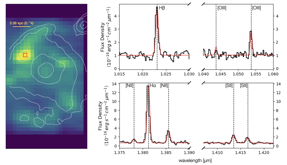
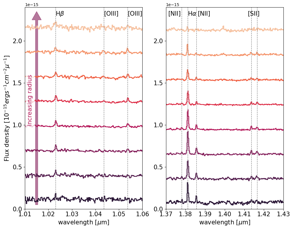
Figure 3: The left panel features a collapsed 2-dimensional image from the data cube centered around the H line at rest-frame 6563 Å. Overlaid white contours indicate the galaxy continuum morphology observed in JWST/NIRCAM F444W imaging. We note that the bright continuum source in the upper-right corner is not associated with the main spiral galaxy; our slit-stepping data spectroscopically confirm it at a slightly lower redshift . The right panels present the 1-dimensional spectrum of a single bright spaxel (shown with the red square at left), zoomed in around the key diagnostic emission lines: H, [O III], [N II], H, and [S II]. Fits to the emission lines are shown in red and are described in the text. All key lines are well detected. Spatial mapping of these emission lines enables characterization of the kinematics, gas-phase metallicity and radial gradients, dust attenuation, star formation rate profile, and nuclear activity in this galaxy. We note that this is only one example of the 43 galaxies observed with our slit-stepping program. -
3.
Stage 2
Stage 2 (“calwebb_spec2”) of JWST’s Science Calibration Pipeline is dedicated to spectroscopic data refinement. Stage 2 applies further instrument-level corrections to slope images, generating calibrated exposures. Our customized processing includes the following steps from this stage: WCS assignment, MSA flagging, extraction of 2D arrays from spectral images, flat field and barshadow correction, flux calibration, and resampling. We do not include the standard pathloss correction step, and instead perform it in post-processing, which we explain in more details in Step 4.iii. -
4.
Stage 3 and post-processing
i. In Stage 3 (“calwebb_spec3”) we perform only the resampling step to create final rectified and combined 2D spectra for each target from calibrated exposures. This step involves taking 2D spectra from each individual detector, resampling them using WCS and distortion information, and combining them into a single undistorted 2D spectrum for each target.ii. A number of outliers, including cosmic rays and other artifacts (e.g., hot pixels) are apparent in the processed 2D spectra, the treatment of which remains an open issue in the standard pipeline. To remove the outliers we apply the astro-SCRAPPY222astro-SCRAPPY: https://zenodo.org/record/1482019 cosmic ray cleaning code, which is based on the L.A.Cosmic algorithm (van Dokkum, 2001).
iii. The role of the pathloss correction function is to account for geometrical and diffraction losses of light. Pathloss correction in the standard pipeline relies on theoretical optical models to correct for pathloss effects for non-centered point sources and those uniformly filling the slit (Ferruit et al., 2022). The current implementation of pathloss correction in the STScI reduction pipeline performs only for a standard number of slitlets (one and three). As the targets in our program are often observed with 3 slitlets, we perform this correction outside of the standard pipeline. We assume a uniformly illuminated slit to correct pathloss effects for extended sources in our slit-stepping program (Nanayakkara et al., 2023). We extract a 1D pathloss function from the pipeline’s uniform pathloss reference file, and correct the 2D spectra of all exposures considering the relevant wavelength range for each target (due to the pathloss model wavelength dependence).
-
5.
Cube construction
Our slit stepping pattern, as described in Section 2.2, consists of 9 dispersion “steps” (02 each) and 7 cross-dispersion dithers (0075 each). Our cube building process combines the 63 individual pointings into a 3D data cube for each target. We first combine 2D spectra in the cross dispersion direction to produce a single 2D spectral slice at each step. We resample individual 2D spectra from each of the 7 dithered exposures (at each dispersion step) onto a common grid with finer spatial pixel scale, such that original pixels are Nyquist sampled. We then take the median of all exposures (with 7 exposures in the central regions, and fewer in the outer 045). A median combination is used to minimize residual effects from cosmic rays, bar shadows, alternating column noise, and other artifacts. This is sufficient for the results presented herein, and this key processing step can be updated with an outlier-rejected weighted mean or other optimized algorithm following future improvements to the earlier pipeline stages. The combination of individual steps is straightforward: we append the 2D spectra at each of the 9 steps into a 3D data cube, with 9 spaxels of 02 in the dispersion direction. The Nyquist sampled cross-dispersion spectra can be rebinned to the original pixel scale, resulting in 0102 spaxels. For analysis and display purposes in this paper, we instead interpolate the data to square spaxels of 008008. This spaxel size corresponds to 0.7 kpc at redshifts –1.7.
2.5 Emission Line Fitting
The results in this paper are based on spatially resolved measurements of the strong rest-frame optical nebular emission lines. The angular resolution is limited by NIRSpec/MSA which undersamples JWST’s point spread function (PSF), especially in the dispersion direction with 02 slitlet width. For the galaxy analyzed in this work, we achieve S/N in the H emission line for individual spaxels spanning 25, with all additional targeted lines ([N II], [S II], H, [O III]) well-detected in bright individual spaxels. The H narrowband flux map and example emission line detections from a single spaxel are shown in Figure 3.
We fit the emission lines within each spaxel using Gaussian profiles, which provide a good fit. The H, [N II] , and [S II] lines are jointly fit with a five-component model plus a linear continuum. All lines are assumed to have the same velocity () and velocity dispersion (). The flux of each line is a free parameter, except for the [N II] doublet whose flux ratio is fixed to the theoretical value of 2.942. The H and [O III] lines are similarly fit with a three-component model with the [O III] doublet flux ratio fixed to 2.984. Example maps of the H flux, velocity, and velocity dispersion are show in Figure 4. The velocity dispersion is corrected for NIRSpec’s spectral resolution ( for the G140H grating) by subtracting the line spread function FWHM in quadrature from the best-fit Gaussian FWHMs. We obtained the instrumental FWHM Å by interpolating the G140H resolution curve across the wavelength range of emission lines used here. In this work we adopt a systemic redshift corresponding to the central region of the galaxy. Velocities in Figure 4 are shown relative to this redshift.
3 Physical Properties
3.1 Disk Kinematics
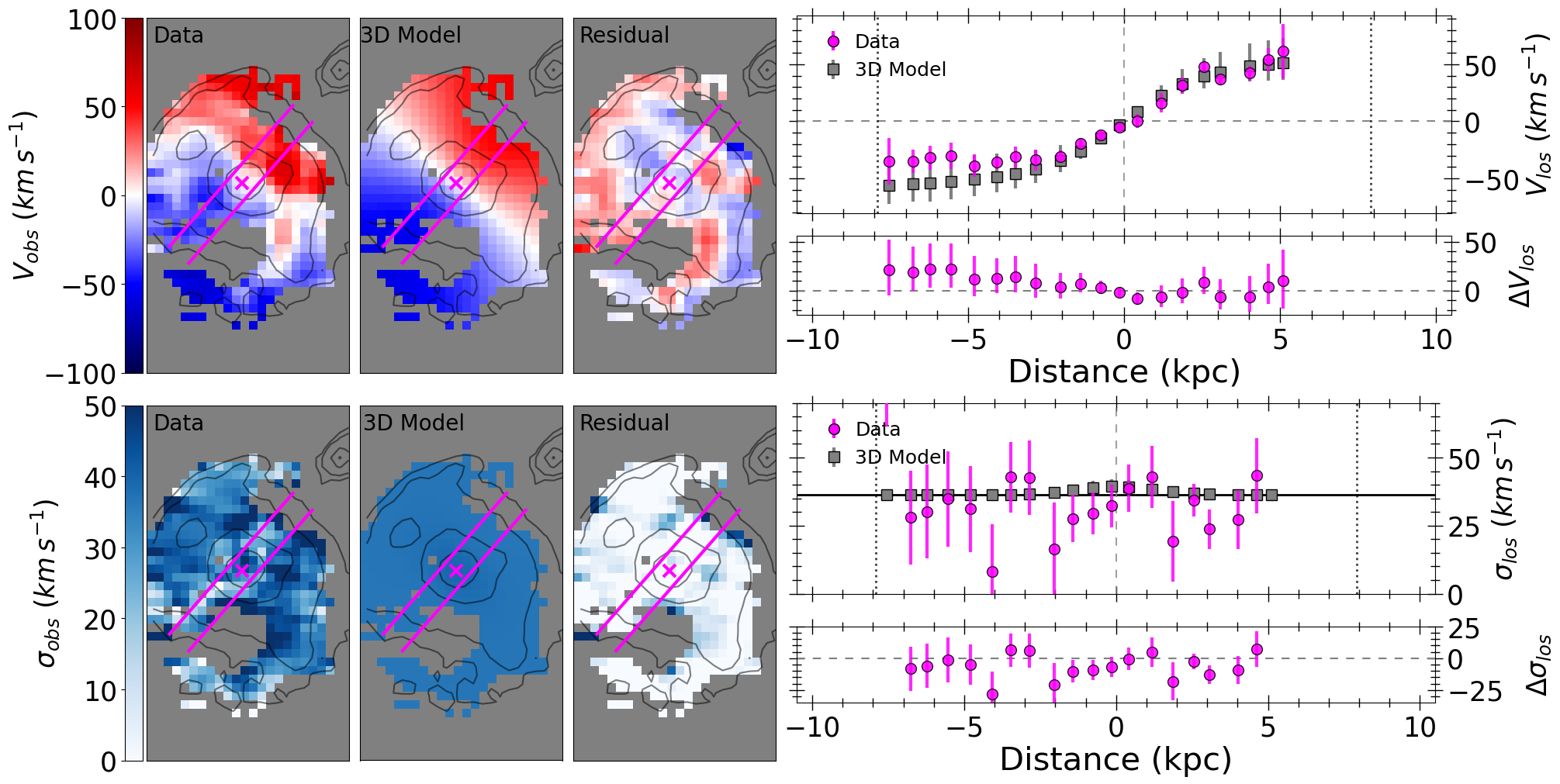
We derive kinematic properties using GalPaK (Bouché et al., 2015), a fitting software optimized for IFU data. We fit the observed H emission in the example target galaxy via forward modeling of galactic disk models, accounting for the line-spread function (LSF) and point-spread function (PSF). The LSF is assumed to be a Gaussian of FWHM Å based on NIRSpec documentation, and the PSF is estimated as an elliptical Gaussian with FWHM , accounting for undersampling by the 02 MSA slitlets. In this paper we assume a rotating disk geometry with a thickness of scale height . The rotation curve is modeled as an arctangent function (Courteau, 1997):
| (3) |
where is the distance along the major axis of the galaxy in the plane of the sky, is the asymptotic velocity in the plane of the disk, is the inclination of the disk, and is the turnover radius. We also model the total line-of-sight velocity dispersion, , which in general has three components added in quadrature: a local isotropic velocity dispersion from the self-gravity of the disk, which is given by for a compact thick disk; a mixing term due to the mixing of velocities along the line of sight in a disk with non-zero thickness; and an intrinsic velocity dispersion (assumed to be isotropic and spatially constant), which represents the dynamical “hotness” of the disk.
Given the rich spiral morphology of H emission, which differs somewhat from the broad-band continuum (Figure 3), we do not model the full 3D flux distribution in the data cube. Instead we fit the velocity and dispersion maps measured from H and the surrounding metal lines as discussed in Section 2.5. We use GalPaK to construct model 2D maps of the velocity and dispersion, and perform a Markov chain Monte Carlo (MCMC) parameter space exploration with the Python software emcee (Foreman-Mackey et al., 2013). A Gaussian prior is adopted for the center of the galaxy, using the position of peak stellar continuum flux in the NIRCam F444W image. The F444W filter corresponds to rest-frame K band ( m) which is expected to be a good tracer of the stellar mass distribution (e.g., Bell & de Jong, 2001). For all other parameters we adopt a flat prior (including, e.g., and ). The likelihood function for our model is defined by agreement with the measured velocity and dispersion maps:
| (4) |
which sums over all spaxels () in both and . Here , , and are the 2D maps of the data, extracted model, and standard deviation measurement uncertainty, respectively. The best-fit and maps along with the residuals () are shown in Figure 4. We also show 1D rotation and velocity disperion curves extracted along the best-fit major axis.
Overall the disk model provides a good fit to the kinematic measurements. The residuals are km s-1 for both and . The best-fit inclination degrees is nearly face on, which is also clear from the imaging data. We note that the source morphology was not used to constrain the fit, such that the model provides an independent confirmation of the face-on disk geometry. While the line-of-sight rotational velocity is tightly constrained by the data, the large inclination correction factor (i.e., ) makes km s-1and relatively uncertain. As such we refrain from detailed analysis of the rotation curve and dynamical mass profile in this galaxy. We note that the value is characteristic of well-settled disks, and agrees well with predictions from the TNG50 simulation at this redshift and stellar mass (Pillepich et al., 2019). Such high values of are also found in the FIRE zoom-in simulations after disk settling (Stern et al., 2021; Gurvich et al., 2023). The majority of our targets have a higher (more edge-on) inclination which allows better constraints on the circular rotation velocity. On the other hand, the velocity dispersion km s-1 is determined with good precision, and this is the key quantity which describes the dynamical state of the disk (e.g., cold thin disk vs. turbulent thick disk). The H and [O III] emission lines give consistent results. In this case the value observed from a nearly face-on inclination corresponds closely with the vertical component of velocity dispersion, which sets the disk scale height.
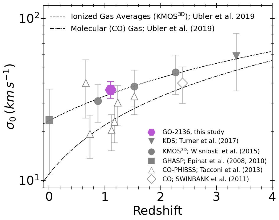
In Figure 5 we compare for the galaxy studied here with average values compiled from various surveys as a function of redshift. Despite the clear spiral disk morphology, the measured is higher than for typical spiral galaxies at , and comparable to the largest values found in the GHASP sample (Epinat et al., 2008). However we find excellent agreement with the average trend seen in KMOS3D (Wisnioski et al., 2015) and other kinematic surveys of ionized gas (e.g., Simons et al., 2017). While this is only a single object whose properties may not be representative, it appears to support the picture of velocity dispersion increasing with redshift. Our best-fit may slightly underestimate the true value due to possible slit illumination effects. Our analysis assumes uniform slit illumination, whereas a partial illumination (e.g., with bright nebular emission concentrated on one side of the 02 slit) would cause the line widths (e.g., ) to appear smaller. Such an effect could cause variation in both the measured and , along with larger scatter in line widths potentially reaching values smaller than the assumed instrument resolution. We would also expect the velocity dispersion measured from H to be systematically smaller than H in the presence of non-uniform slit illumination (due to the smaller PSF at shorter wavelengths). Instead we find relatively small scatter in velocity dispersion, with values from H and [O III] being slightly larger on average (by %) than those measured from H in radial bins. We thus conclude that the bias from non-uniform slit illumination is comparable or smaller than the measurement uncertainty. Future efforts may be able to better quantify the effects of non-uniform slit illumination by forward-modeling the light distribution (e.g., based on imaging or grism spectroscopy).
In summary we find that the dynamical state of the disk, as indicated by local velocity dispersion, is more turbulent than in spirals and comparable to that inferred from large ground-based samples at (e.g., Wisnioski et al., 2015; Stott et al., 2016). In contrast to typical ground-based data, our measurement of is especially robust to beam smearing effects, thanks to the nearly face-on inclination and the exquisite space-based point-spread function of the data. The best-fit kinematic major axis (PA degrees) and disk inclination ( degrees) are used to construct deprojected radial bins in the following sections.
3.2 Flux Ratios and BPT Diagram
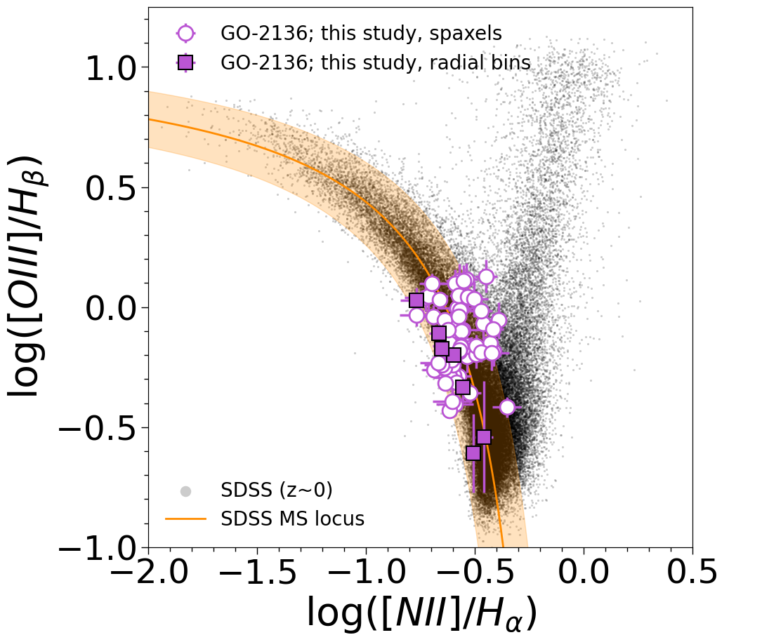
To classify the dominant energy source of line emission within this galaxy and to establish the degree of nuclear supermassive black hole activity, we examined the Baldwin–Phillips–Terlevich (BPT) diagram (Baldwin et al., 1981) of [O III]/H versus [N II]/H flux ratios. Given the moderate S/N of [O III] and H emission within typical individual spaxels, we use radial annular bins. The bins are constructed using the deprojected radius based on the best-fit inclination and position angle derived from our kinematic disk model (Section 3.1). We adopt bins of 1.7 kpc (02 arcseconds) in deprojected radius, corresponding to the MSA slit width. We stack the spectra in each bin and fit the emission profiles to calculate the radially averaged flux ratios across the galaxy. We verified that the fit residuals are in good agreement with the estimated error spectra. Figure 7 shows the resulting BPT diagram measured for both radial bins and individual bright spaxels throughout the galaxy. For individual spaxels shown in the BPT diagram in Figure 7 we adopt a threshold of S/N5 in all requisite lines, exclude spaxels near the edges and those far outside the boundary of the galaxy as indicated by F444W photometric contours, and exclude spaxels with velocity or dispersion measurements near the fitting boundaries (indicating spurious fits).
Our data show that nebular emission within this galaxy is dominated by star formation, as all spatially-resolved regions lie well within the star-forming locus of the BPT diagram. The galaxy follows the star-forming locus within radial bins, and we can also clearly verify that prominent “clumps” of H emission seen in Figure 3 are indeed driven by active star formation. Notably the PSF of JWST allows us to resolve the central kpc with minimal beam smearing from emission at larger radii. We see no evidence of AGN contribution even within this central resolution element. We can place a rough limit on the contribution of nuclear emission driven by supermassive black hole accretion: assuming a central AGN with a flux ratio log([O III]/H) , a contribution of 20% of the Balmer line fluxes from such an AGN in the central resolution element would be readily detected (approximately tripling the [O III] flux relative to the star-forming locus in the central resolution element). The central bin contains only 3.8% of the total observed H flux (although a larger fraction of total intrinsic flux accounting for attenuation; see Section 3.4). Taking 20% of this, we arrive at a conservative estimate that % of the total observed H flux textcolormagentacould be associated with an AGN. The corresponding limit on the central spatial resolution element is approximately half of this (%). We conclude that either there is very little supermassive black hole accretion in this galaxy, or that any accretion-driven luminosity must be heavily dust-obscured. This sensitive limit highlights the power of high angular resolution observations to detect low-luminosity AGN (e.g., Wright et al., 2010) even in galaxies dominated by star formation.
3.3 Gas-Phase Metallicity Gradient
We now turn to the gas-phase metallicity as a function of radius using the same bins described in Section 3.2. We estimate metallicity using the locally calibrated strong-line relations of Pettini & Pagel (2004, PP04) and Curti et al. (2017, C17) using the available [N II]/H and [O III]/H line ratios. Specifically we consider the
diagnostics. While numerous other calibrations are available in the literature, including some based directly on galaxies at similar (Jones et al., 2015a; Sanders et al., 2020), the adopted calibration has little effect on the conclusions of this section. We use PP04 and C17 in order to illustrate both the numerical differences and qualitatively similar conclusions.
In Figure 8 we show the gas-phase metallicity as a function of deprojected radius (using the mean radius of spaxels within each bin). The top panel plots results from all three diagnostics (O3N2, N2, and R3) using the C17 calibrations. All show similar negative gradients, reflecting the radial trends in emission line flux ratios apparent in Figures 6 and 7. We additionally show a linear fit for the O3N2 index, which gives a best-fit gradient slope dex kpc-1. The independent N2-based measurement differs systematically in normalization by dex, while R3-based measurement is consistent with the O3N2-based measurement. Both are within the known scatter in these relations (e.g., Kewley et al., 2019), and display a consistent gradient slope. Independent line ratios thus give a consistent overall metallicity and radial gradient.
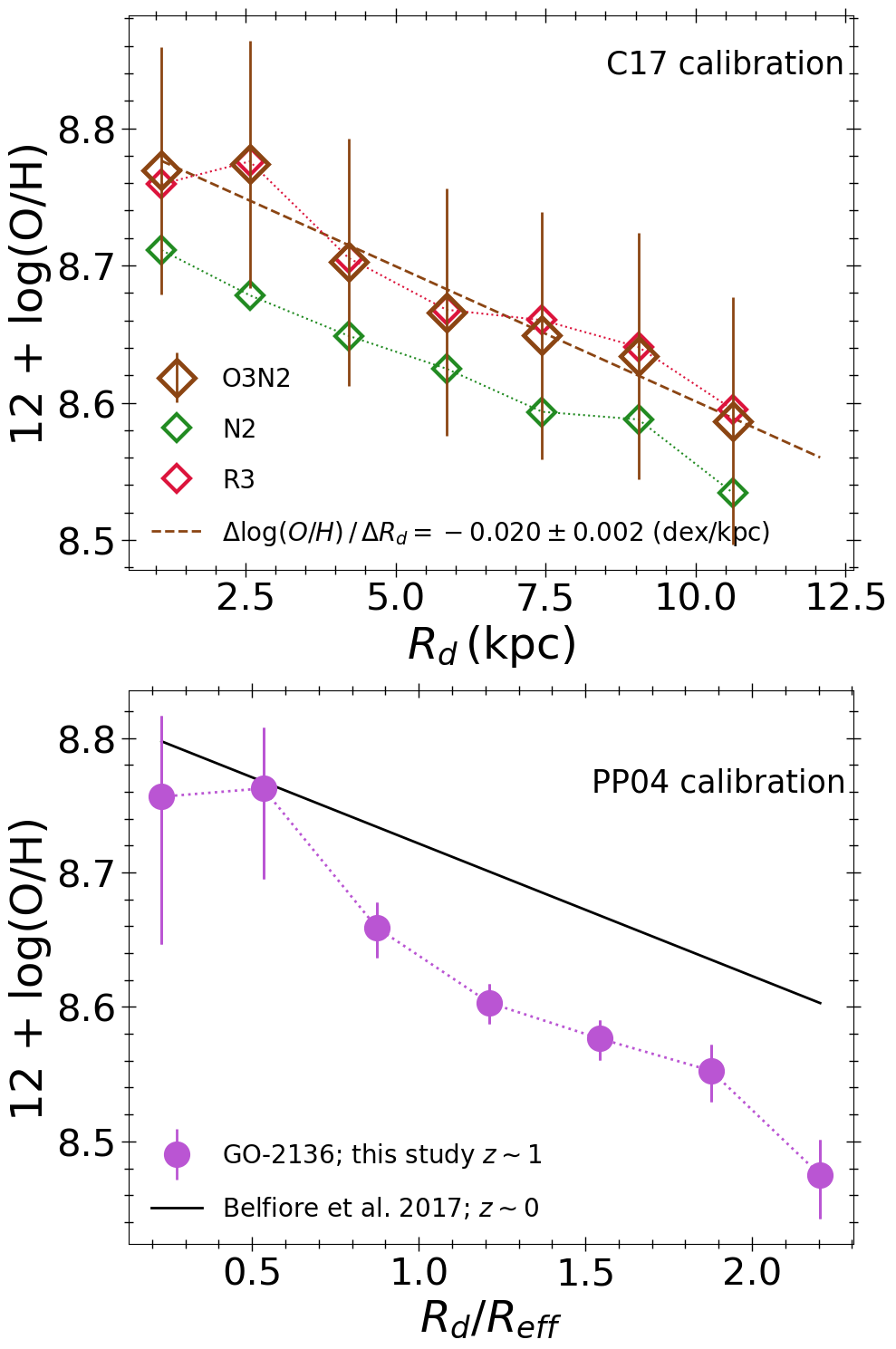
In the lower panel of Figure 8 we make a direct comparison with typical metallicity gradients measured for spiral galaxies by Belfiore et al. (2017), at the same stellar mass range (–10.5) as our target galaxy (). For consistency we compare results from the same metallicity calibration (i.e., O3N2 from PP04), normalized to the effective radius (with kpc for our target; Section 3.5). The PP04 calibration gives a larger total O/H range and steeper metallicity gradient compared to C17, while we emphasize the conclusion of a negative radial gradient remains robust.

The observed metallicity gradient is in accordance with the kinematic results which indicate a well-ordered rotating disk. Gas mixing due to turbulence, mergers, feedback-driven galactic fountains, or other factors is expected to reduce or eliminate any radial gradient (e.g., Ma et al., 2017; Rich et al., 2012; Kewley et al., 2010). The strong gradient in this galaxy implies little influence from such effects. At fixed stellar mass , the metallicity gradient of our example galaxy at is steeper (more negative slope) than the average at from Belfiore et al. (2017) while both have similar central metallicities. However we caution that the galaxy is a case study and is not necessarily representative of the general population. Its SFR places it below the main sequence at (Figure 1), such that stellar feedback and other gas-mixing process may be relatively modest. Preliminary analysis indicates that it is in the steepest quartile of dex gradient slopes within the sample observed by this program (Ju et al., in prep). We also note that this is not an evolutionary comparison, as our target galaxy is expected to grow more massive by . We leave a detailed analysis of our full sample and its chemical evolution for future work; here we have demonstrated the ability to measure metallicity gradients at a precision suitable for comparison with galaxies.
3.4 Dust Attenuation Gradient
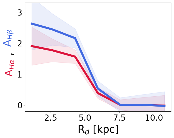
Optical H I emission lines are a valuable diagnostic for characterizing dust attenuation in galaxies. The Balmer decrement, defined as the ratio of H/H, is a commonly used metric to determine the degree of attenuation and reddening (e.g., Charlot & Fall, 2000). The attenuation is determined by quantifying its deviation from the theoretical value (Baker & Menzel, 1938; Osterbrock & Ferland, 2006). Assuming Case B recombination with electron temperature 104 K and electron density of 102 cm-3, the expected Balmer decrement value is 2.86 (Osterbrock & Ferland, 2006; Storey & Hummer, 1995). In each radial bin, we measure the integrated H/H flux ratios from the best-fit line profiles. Figure 9 shows the resulting Balmer decrement profile of the galaxy. It displays a clear negative radial trend, indicating larger attenuation in the central regions.
We infer attenuation AHα and AHβ from the measured Balmer decrement following standard methods. The attenuation is related to the color excess E(B-V) as A E(B-V), where kλ corresponds to the reddening curve. The color excess E(B-V) can be measured from:
| (5) |
where 2.86 is the assumed intrinsic H/H flux ratio. It is necessary to assume a reddening law for kλ. For consistency with previous studies (e.g., Nelson et al., 2016b), we adopt the Calzetti et al. (2000) reddening law (with kHα = 3.33 and kHβ = 4.60). The resulting attenuation versus radius for both H and H are shown in the right panel of Figure 9. We note that the choice of reddening law can affect the derived attenuation (e.g., AHα) – although this effect is minor in the optical wavelength range, whereas the color excess and radial profile shape are relatively robust. We find a strong radial trend with higher attenuation in the central kpc. This is similar to the results for massive disk galaxies found by Tacchella et al. (2018) using other methods to determine attenuation.
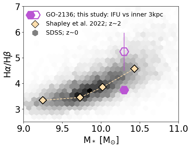
Previous studies of the Balmer decrement in galaxies have noted a positive correlation with stellar mass, suggesting that more massive galaxies typically have larger attenuation from dust in their interstellar medium (e.g. van Dokkum et al., 2005; Ly et al., 2012; Kashino et al., 2013; Domínguez et al., 2013; Price et al., 2014; McLure et al., 2018; Shapley et al., 2022). These studies also indicate no significant evolution in dust attenuation at fixed mass up to . Moreover, alternative assessments of dust attenuation through indicators such as infrared excess IRX, optical attenuation AV, and/or ultraviolet attenuation A1600 and spectral slope have reported consistent findings (e.g., Wuyts et al., 2013; Heinis et al., 2014; Bouwens et al., 2016; Bourne et al., 2017; Whitaker et al., 2017; McLure et al., 2018). In Figure 10 we compare the Balmer decrement of our target from both the integrated spectrum and from the central kpc (to mimic single-slit or fiber observations), with the results from galaxies at lower and higher redshifts (: SDSS; : MOSDEF, Shapley et al. 2022). There is a striking difference between the integrated spectrum and the central kpc, with the central Balmer decrement being nearly 1.5 the integrated value. This central region is representative of the area covered by a single NIRSpec slitlet (Figure 1). This comparison shows that single-slit or otherwise centrally concentrated observations can lead to an inaccurate assessment of the overall dust attenuation in the galaxy. The integrated measurement of our galaxy exhibits a smaller Balmer decrement compared to the average observed at a fixed stellar mass in both the SDSS sample and the MOSDEF sample, although it is within the scatter seen in SDSS. Lorenz et al. (2023) found no significant correlation between the Balmer decrement and galaxy viewing angle, suggesting that the face-on inclination of our target is not responsible for the moderately low attenuation. However they also noted a trend of attenuation increasing with star formation rate. Our target galaxy has a SFR of 3 yr-1 which places it below the typical sSFR at its redshift (e.g., Whitaker et al. 2012; Figure 1), which may partly explain the lower attenuation.
3.5 Surface Brightness Profile
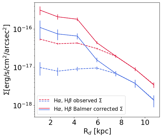
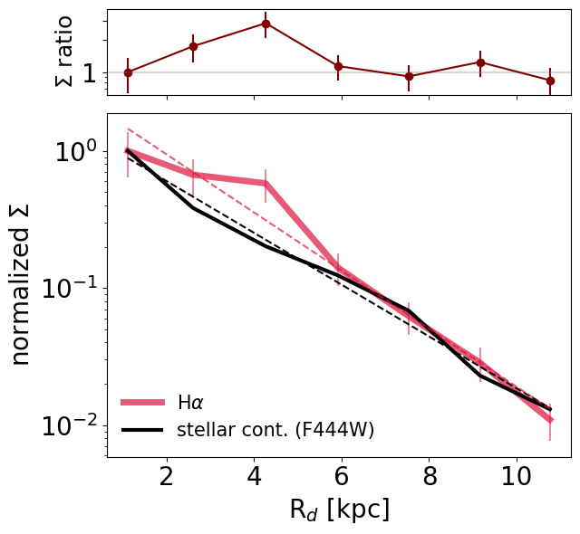
We now examine the surface density profile of star formation, as traced by attenuation-corrected H emission, and compare it with the stellar continuum. This provides insight into the structural evolution and radial size growth of this galaxy. From the measurements described in Section 3.4, we obtain intrinsic H and H fluxes as a function of radius via
Figure 11 shows the observed and intrinsic (i.e., attenuation corrected) radial surface brightness profiles for both H and H. The observed profiles are relatively flat in the inner 5 kpc, with larger Balmer decrements indicating more attenuation in the central regions (demonstrated in Figure 9). The average spatial profiles found at by Nelson et al. (2016b) similarly show a flattening of the inner H profile at high masses, with larger Balmer decrements in the central regions. However the stacked profiles in Nelson et al. (2016b) exhibit centrally peaked H profiles across all mass bins, in contrast to the flatter inner profile seen in Figure 11. The attenuation-corrected profiles of our target galaxy do show a clear central peak, with an approximately exponential surface brightness profile. This is indicative of star formation continuing to build an exponential disk. We find no indication of significant in situ bulge formation (in which case we would expect an elevated central surface brightness relative to the overall exponential profile), nor of inside-out quenching (in which case we would expect a lower corrected central surface brightness; e.g., Tacchella et al. 2018; Lin et al. 2019).
Our target is covered by JWST/NIRCam imaging from the CEERS survey (Finkelstein et al., 2023), which we use to trace the stellar surface brightness profile. Of particular interest is the F444W band, which measures stellar continuum at a rest-frame of 2.1 m (i.e., rest-frame K band). We use this as a proxy for the stellar mass surface density, as the mass-to-light ratio varies by only a factor at K band (e.g., Bell & de Jong, 2001; McGaugh & Schombert, 2014), which is minimal given the factor 100 in surface brightness probed here. The Balmer decrement profile (Figure 9) additionally suggests relatively little dust attenuation AK at these wavelengths. The F444W image is first rescaled to the same pixel size as the NIRSpec data cube, after which we extract the radial surface brightness profile. In Figure 11 we compare the dust corrected H surface brightness profile (which traces the SFR) to that of rest-frame K band stellar continuum (which traces stellar mass). Both are normalized at the central bin for ease of comparison. The H and stellar continuum both follow an approximately exponential profile with similar scale length, decreasing by a factor of over 10 kpc in radius. An exponential profile fit gives scale length kpc for the continuum, corresponding to a half-light or effective radius of kpc. This is consistent with the size-mass relationship for late type galaxies at , which indicate typical –5 kpc at the mass of our target (van der Wel et al., 2014). Additionally we note the half-light radius of our target galaxy is similar to that of the Milky Way (4–6 kpc; Bland-Hawthorn & Gerhard 2016; Lian et al. 2024).
The H (= SFR) and continuum (= stellar mass) scale lengths are close and mutually consistent within 1.2, with H being % smaller than the continuum. At face value this is in contrast to the picture of “inside-out” disk growth whereby the H scale length is larger than that of the stars. For example, Nelson et al. (2016a) report that H scale lengths of their sample of galaxies are on average 14% larger than the observed 1.4 m continuum for similar redshift and stellar mass (–10.5), although is only 4% larger and consistent within uncertainties. While our measurements are compatible with this level inside-out growth at the level, overall it appears that the ongoing star formation is not significantly altering the galaxy’s scale length. We conclude that this galaxy stellar component is growing proportionally more massive on average at all radii.
Figure 11 also shows the ratio of H and stellar continuum radial surface brightness profiles, normalized at the central bin. This ratio is proportional to the specific SFR (sSFR). The most notable deviation from a constant sSFR profile is a clear excess of H emission around 4 kpc, while elsewhere the profiles align closely. The excess reaches up to three times higher H surface brightness relative to the continuum.
One possible explanation for this H excess emission may be prominent clumps within the spiral arms, including a bright clump in the upper left and a fainter clump in the upper right quadrant in Figure 3. However, the Balmer decrement indicates significant dust obscuration in the inner 4 kpc, such that the morphology seen in Figure 3 differs from the more centrally-concentrated profile we obtain after attenuation correction. To further explore the nature of the excess emission at 4 kpc, we split the cube into “upper” and “lower” halves. After correcting for dust, the H surface brightness density in the lower half is higher than that of the upper half (which contains the brightest observed regions). We find excess in attenuation-corrected H surface brightness profiles in both halves, indicating that it is not caused solely by the discrete bright regions. Instead it may suggest the presence of a Lindblad resonance driving a ring of star formation at this radius (e.g., Buta & Combes, 1996).
4 Discussion and Conclusions
We have presented the design and initial results of the MSA-3D program which obtained spatially resolved spectroscopy for 43 star-forming galaxies at , using a slit-stepping observing strategy with JWST/NIRSpec’s MSA. We illustrate the data quality with a case study of a spiral disk galaxy at . This galaxy exhibits features typical of late-type spirals in the nearby universe: prominent spiral arm morphology (Figures 1, 3), rotation-dominated kinematics (Section 3.1; Figure 4), a negative gas-phase metallicity gradient (Section 3.3; Figure 8), and exponential surface brightness profiles in both stellar continuum and star formation (Section 3.5; Figure 6). These results collectively demonstrate the ability of our slit-stepping methodology to characterize galaxies via emission line mapping with 1 kpc resolution. We emphasize that the galaxy analyzed in detail in this paper is typical of the data quality within the larger sample. We refer readers to Ju et al. (in prep) for analysis of the metallicity gradients measured for 26 of our 43 targets, as well as maps of the H flux and kinematics.
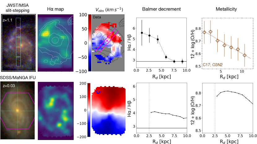
The quality of emission line measurements we achieve with MSA-3D at is comparable to that of MaNGA (Bundy et al., 2015; Drory et al., 2015) and other surveys of galaxies. In Figure 12 we make a direct comparison of our MSA-3D case study target with an example galaxy from MaNGA (MaNGA ID 12-129618, plate-IFU 7495-12704) at . This MaNGA target is chosen for comparison on the basis of similar spiral morphology and stellar mass (). Figure 12 shows the color image, H emission map, H-based gas velocity field, Balmer decrement (i.e., H/H flux ratio), and radial metallicity gradient for both the and galaxies. We note that the Balmer decrement and metallicity gradient are measured from deprojected radial bins using the same methods as described in Section 3 (while the H flux and velocity maps are taken directly from the MaNGA DAP output; Westfall et al. 2019). A key difference which is not shown is that the MaNGA target contains an AGN, with LINER emission identified via the BPT diagram at kpc. Our target galaxy has no detected AGN emission despite sensitive limits (e.g., % of observed H flux; Figures 6, 7) as described in Section 3.2. An AGN contribution at the level seen in the MaNGA target would be readily detected in our MSA-3D data. Other than nuclear activity, both galaxies show similar structure: spiral morphology, rotating disk kinematics, higher dust attenuation toward the central regions, and gas metallicity decreasing with radius. The data quality is able to reveal subtle quantitative differences in properties such as the radial profiles of the Balmer decrement and metallicity. This comparison demonstrates the ability to make meaningful and detailed comparisons of our sample with the galaxy population. JWST/NIRSpec slit-stepping data are thus powerful for galaxy evolution studies.
We emphasize that the MSA-3D slit-stepping data enable excellent spatially resolved measurements for individual galaxies, such as the one studied here. This represents a significant advance over previous methods, such as the stacking technique utilized with Hubble Space Telescope grisms, which combined high-resolution optical imaging with low-resolution GRISM spectroscopy to measure radial Balmer decrement and star formation profiles (Nelson et al., 2016a, b). Previous state-of-the-art IFS studies at relied on hour integrations with ground-based telescopes and adaptive optics (e.g., Tacchella et al., 2018; Genzel et al., 2020). These deep AO studies typically focus on H emission (and the nearby [N II] and [S II]), whereas our MSA-3D data cover additional key lines such as [O III] and H, or [S III] and other features depending on the redshift and slit mask placement (Table 1). The wavelength coverage of our MSA-3D observations is largely inaccessible to current AO systems, yet it is invaluable for accurately establishing the spatially resolved dust attenuation, AGN contributions, metallicity, and other properties. Indeed, to our knowledge the results shown in this paper represent the most robust resolved Balmer decrement, dust-corrected H (i.e., SFR), and metallicity maps ever obtained for a galaxy.
An important conclusion from initial analyses of our MSA-3D program is that the slit-stepping strategy with NIRSpec’s MSA is a highly effective and efficient method to observe large samples of galaxies across cosmic time.
As discussed in Section 2.3, slit-stepping is the most cost-effective approach for IFS surveys of populations with projected number density arcmin-2, which can take advantage of NIRSpec/MSA’s multiplexing capability and sensitivity. Slit-stepping is complementary to NIRSpec’s IFU mode, which provides finer spatial sampling and is powerful for studying objects which are rare on the sky. This includes gravitational lenses (e.g., Rigby et al., 2023) and extremely luminous systems (e.g., Marshall et al., 2023). Four programs have adopted slit-stepping strategies to date. Our 30 hour JWST Cycle 1 program has already delivered standalone data for 43 galaxies at with exquisite sensitivity, wavelength coverage, and spatial and spectral resolution. A followup Cycle 2 program (JWST-GO-3426) by our team recently obtained comparable slit-stepping IFS data for 42 galaxies at within a single pointing. Two programs from another team have obtained slit-stepping observations of 56 galaxies at –5 (JWST-GO-2123), and 250 galaxies at (JWST-GO-4291), using a different and complementary dithering strategy. Collectively these four programs represent an investment of just over 200 hours of JWST time allocation – less than the GA-NIFS program which is observing 50 galaxies with the IFU mode.
Given the remarkable efficiency of MSA slit-stepping and its demonstrated success via our MSA-3D program, we advocate for future programs to comprehensively survey the galaxy population across cosmic time using this method. The four programs carried out to date are an excellent start, yet represent a modest subset of cosmic times and galaxy properties (e.g., mass and star formation rate). An IFS sample size equivalent to the KMOS3D survey (739 galaxies at –2.7; Wisnioski et al., 2019) would require approximately 600 hours at the depth of our MSA-3D program, which delivers broader wavelength coverage and 5–10 times better angular resolution than KMOS3D. Such a sample can be obtained in hours at the shallower depth adopted by the JWST-GO-4291 program. A sample of this size is out of reach for JWST’s IFU modes in its limited mission lifetime, yet it is achievable with MSA slit-stepping. Despite the clear advantages, however, slit-stepping is not an officially supported observing mode and the standard data reduction pipelines are not equipped to handle it. We are mitigating this by publicly releasing our custom pipeline (Section 2.4) and example data products. While we are already addressing the main challenges associated with data processing, we also advocate for further investment in software infrastructure to optimize the scientific return of slit-stepping surveys.
ACKNOWLEDGEMENTS
We thank B. Rauscher for developing the NSClean algorithm and making it available. We thank Keerthi G. C. Vasan for their valuable input. This work is based on observations made with the NASA/ESA/CSA James Webb Space Telescope. The data were obtained from the Mikulski Archive for Space Telescopes at the Space Telescope Science Institute, which is operated by the Association of Universities for Research in Astronomy, Inc., under NASA contract NAS 5-03127 for JWST. These observations are associated with program JWST-GO-2136. We acknowledge financial support from NASA through grant JWST-GO-2136. This work made use of observations and catalogs from the 3D-HST Treasury Program (GO 12177 and 12328) with the NASA/ESA Hubble Space Telescope, which is operated by the Association of Universities for Research in Astronomy, Inc., under NASA contract NAS5-26555. XW and MJ are supported by the National Natural Science Foundation of China (grant 12373009), the CAS Project for Young Scientists in Basic Research Grant No. YSBR-062, the Fundamental Research Funds for the Central Universities, the Xiaomi Young Talents Program, and the science research grant from the China Manned Space Project. CAFG was supported by NSF through grants AST-2108230 and AST-2307327; by NASA through grant 21-ATP21-0036; and by STScI through grant JWST-AR-03252.001-A. J.M.E.S. acknowledges financial support from the European Research Council (ERC) Advanced Grant under the European Union’s Horizon Europe research and innovation programme (grant agreement AdG GALPHYS, No. 101055023).
References
- Abazajian et al. (2009) Abazajian, K. N., Adelman-McCarthy, J. K., Agüeros, M. A., et al. 2009, ApJS, 182, 543
- Baker & Menzel (1938) Baker, J. G., & Menzel, D. H. 1938, ApJ, 88, 52
- Baldwin et al. (1981) Baldwin, J. A., Phillips, M. M., & Terlevich, R. 1981, PASP, 93, 5
- Belfiore et al. (2017) Belfiore, F., Maiolino, R., Tremonti, C., et al. 2017, MNRAS, 469, 151
- Bell & de Jong (2001) Bell, E. F., & de Jong, R. S. 2001, ApJ, 550, 212
- Belli et al. (2017) Belli, S., Genzel, R., Förster Schreiber, N. M., et al. 2017, ApJ, 841, L6
- Bennett et al. (2014) Bennett, C. L., Larson, D., Weiland, J. L., & Hinshaw, G. 2014, ApJ, 794, 135
- Bland-Hawthorn & Gerhard (2016) Bland-Hawthorn, J., & Gerhard, O. 2016, ARA&A, 54, 529
- Böker et al. (2023) Böker, T., Beck, T. L., Birkmann, S. M., et al. 2023, PASP, 135, 038001
- Bouché et al. (2015) Bouché, N., Carfantan, H., Schroetter, I., Michel-Dansac, L., & Contini, T. 2015, AJ, 150, 92
- Bourne et al. (2017) Bourne, N., Dunlop, J. S., Merlin, E., et al. 2017, MNRAS, 467, 1360
- Bouwens et al. (2016) Bouwens, R. J., Aravena, M., Decarli, R., et al. 2016, ApJ, 833, 72
- Brammer et al. (2012) Brammer, G. B., van Dokkum, P. G., Franx, M., et al. 2012, ApJS, 200, 13
- Brennan et al. (2017) Brennan, R., Pandya, V., Somerville, R. S., et al. 2017, MNRAS, 465, 619
- Bundy et al. (2015) Bundy, K., Bershady, M. A., Law, D. R., et al. 2015, ApJ, 798, 7
- Burkert et al. (2016) Burkert, A., Förster Schreiber, N. M., Genzel, R., et al. 2016, ApJ, 826, 214
- Buta & Combes (1996) Buta, R., & Combes, F. 1996, Fund. Cosmic Phys., 17, 95
- Byrne et al. (2023) Byrne, L., Faucher-Giguère, C.-A., Stern, J., et al. 2023, MNRAS, 520, 722
- Calzetti et al. (2000) Calzetti, D., Armus, L., Bohlin, R. C., et al. 2000, ApJ, 533, 682
- Charlot & Fall (2000) Charlot, S., & Fall, S. M. 2000, ApJ, 539, 718
- Courteau (1997) Courteau, S. 1997, AJ, 114, 2402
- Curti et al. (2017) Curti, M., Cresci, G., Mannucci, F., et al. 2017, MNRAS, 465, 1384
- Curti et al. (2020) Curti, M., Maiolino, R., Cirasuolo, M., et al. 2020, MNRAS, 492, 821
- Davies et al. (2011) Davies, R., Förster Schreiber, N. M., Cresci, G., et al. 2011, ApJ, 741, 69
- Dekel et al. (2009) Dekel, A., Sari, R., & Ceverino, D. 2009, ApJ, 703, 785
- Domínguez et al. (2013) Domínguez, A., Siana, B., Henry, A. L., et al. 2013, ApJ, 763, 145
- Drory et al. (2015) Drory, N., MacDonald, N., Bershady, M. A., et al. 2015, AJ, 149, 77
- Elmegreen & Elmegreen (2006) Elmegreen, B. G., & Elmegreen, D. M. 2006, ApJ, 650, 644
- Epinat et al. (2008) Epinat, B., Amram, P., Marcelin, M., et al. 2008, MNRAS, 388, 500
- Epinat et al. (2009) Epinat, B., Contini, T., Le Fèvre, O., et al. 2009, A&A, 504, 789
- Epinat et al. (2012) Epinat, B., Tasca, L., Amram, P., et al. 2012, A&A, 539, A92
- Espejo Salcedo et al. (2022) Espejo Salcedo, J. M., Glazebrook, K., Fisher, D. B., et al. 2022, MNRAS, 509, 2318
- Faucher-Giguère & Oh (2023) Faucher-Giguère, C.-A., & Oh, S. P. 2023, ARA&A, 61, 131
- Faucher-Giguère et al. (2013) Faucher-Giguère, C.-A., Quataert, E., & Hopkins, P. F. 2013, MNRAS, 433, 1970
- Ferruit et al. (2022) Ferruit, P., Jakobsen, P., Giardino, G., et al. 2022, A&A, 661, A81
- Finkelstein et al. (2023) Finkelstein, S. L., Bagley, M. B., Ferguson, H. C., et al. 2023, ApJ, 946, L13
- Forbes et al. (2023) Forbes, J. C., Emami, R., Somerville, R. S., et al. 2023, ApJ, 948, 107
- Foreman-Mackey et al. (2013) Foreman-Mackey, D., Hogg, D. W., Lang, D., & Goodman, J. 2013, PASP, 125, 306
- Förster Schreiber & Wuyts (2020) Förster Schreiber, N. M., & Wuyts, S. 2020, ARA&A, 58, 661
- Förster Schreiber et al. (2009) Förster Schreiber, N. M., Genzel, R., Bouché, N., et al. 2009, ApJ, 706, 1364
- Förster Schreiber et al. (2011) Förster Schreiber, N. M., Shapley, A. E., Genzel, R., et al. 2011, ApJ, 739, 45
- Förster Schreiber et al. (2018) Förster Schreiber, N. M., Renzini, A., Mancini, C., et al. 2018, ApJS, 238, 21
- Freeman (1970) Freeman, K. C. 1970, ApJ, 160, 811
- Genzel et al. (2006) Genzel, R., Tacconi, L. J., Eisenhauer, F., et al. 2006, Nature, 442, 786
- Genzel et al. (2008) Genzel, R., Burkert, A., Bouché, N., et al. 2008, ApJ, 687, 59
- Genzel et al. (2013) Genzel, R., Tacconi, L. J., Kurk, J., et al. 2013, ApJ, 773, 68
- Genzel et al. (2020) Genzel, R., Price, S. H., Übler, H., et al. 2020, ApJ, 902, 98
- Gibson et al. (2013) Gibson, B. K., Pilkington, K., Brook, C. B., Stinson, G. S., & Bailin, J. 2013, A&A, 554, A47
- Glazebrook (2013) Glazebrook, K. 2013, PASA, 30, e056
- Green & Olszewski (2020) Green, J. D., & Olszewski, H. 2020, IR Snowball Occurrences in WFC3/IR: 2009-2019, Instrument Science Report WFC3 2020-3, ,
- Guo et al. (2015) Guo, Y., Ferguson, H. C., Bell, E. F., et al. 2015, ApJ, 800, 39
- Gurvich et al. (2023) Gurvich, A. B., Stern, J., Faucher-Giguère, C.-A., et al. 2023, MNRAS, 519, 2598
- Hafen et al. (2022) Hafen, Z., Stern, J., Bullock, J., et al. 2022, MNRAS, 514, 5056
- Hamilton-Campos et al. (2023) Hamilton-Campos, K. A., Simons, R. C., Peeples, M. S., Snyder, G. F., & Heckman, T. M. 2023, arXiv e-prints, arXiv:2303.04171
- Heinis et al. (2014) Heinis, S., Buat, V., Béthermin, M., et al. 2014, MNRAS, 437, 1268
- Hemler et al. (2021) Hemler, Z. S., Torrey, P., Qi, J., et al. 2021, MNRAS, 506, 3024
- Hirtenstein et al. (2019) Hirtenstein, J., Jones, T., Wang, X., et al. 2019, ApJ, 880, 54
- Ho et al. (2017) Ho, I. T., Seibert, M., Meidt, S. E., et al. 2017, ApJ, 846, 39
- Hopkins et al. (2023) Hopkins, P. F., Gurvich, A. B., Shen, X., et al. 2023, MNRAS, arXiv:2301.08263
- Hubble (1926) Hubble, E. P. 1926, ApJ, 64, 321
- Jakobsen et al. (2022) Jakobsen, P., Ferruit, P., Alves de Oliveira, C., et al. 2022, A&A, 661, A80
- Jones et al. (2021) Jones, G. C., Vergani, D., Romano, M., et al. 2021, MNRAS, 507, 3540
- Jones et al. (2013) Jones, T., Ellis, R. S., Richard, J., & Jullo, E. 2013, ApJ, 765, 48
- Jones et al. (2015a) Jones, T., Martin, C., & Cooper, M. C. 2015a, ApJ, 813, 126
- Jones et al. (2015b) Jones, T., Wang, X., Schmidt, K. B., et al. 2015b, AJ, 149, 107
- Jones et al. (2010) Jones, T. A., Swinbank, A. M., Ellis, R. S., Richard, J., & Stark, D. P. 2010, MNRAS, 404, 1247
- Ju et al. (2022) Ju, M., Yin, J., Liu, R., et al. 2022, ApJ, 938, 96
- Kashino et al. (2013) Kashino, D., Silverman, J. D., Rodighiero, G., et al. 2013, ApJ, 777, L8
- Kassin et al. (2012) Kassin, S. A., Weiner, B. J., Faber, S. M., et al. 2012, ApJ, 758, 106
- Kennicutt (1998) Kennicutt, Robert C., J. 1998, ARA&A, 36, 189
- Kewley et al. (2013) Kewley, L. J., Dopita, M. A., Leitherer, C., et al. 2013, ApJ, 774, 100
- Kewley et al. (2019) Kewley, L. J., Nicholls, D. C., & Sutherland, R. S. 2019, ARA&A, 57, 511
- Kewley et al. (2010) Kewley, L. J., Rupke, D., Zahid, H. J., Geller, M. J., & Barton, E. J. 2010, ApJ, 721, L48
- Koekemoer et al. (2011) Koekemoer, A. M., Faber, S. M., Ferguson, H. C., et al. 2011, ApJS, 197, 36
- Kriek et al. (2015) Kriek, M., Shapley, A. E., Reddy, N. A., et al. 2015, ApJS, 218, 15
- Kuhn et al. (2024) Kuhn, V., Guo, Y., Martin, A., et al. 2024, ApJ, 968, L15
- Leethochawalit et al. (2016) Leethochawalit, N., Jones, T. A., Ellis, R. S., et al. 2016, ApJ, 820, 84
- Lian et al. (2024) Lian, J., Zasowski, G., Chen, B., et al. 2024, arXiv e-prints, arXiv:2406.05604
- Lin et al. (2019) Lin, L., Hsieh, B.-C., Pan, H.-A., et al. 2019, ApJ, 872, 50
- Livermore et al. (2015) Livermore, R. C., Jones, T. A., Richard, J., et al. 2015, MNRAS, 450, 1812
- Lorenz et al. (2023) Lorenz, B., Kriek, M., Shapley, A. E., et al. 2023, ApJ, 951, 29
- Ly et al. (2012) Ly, C., Malkan, M. A., Kashikawa, N., et al. 2012, ApJ, 747, L16
- Ma et al. (2017) Ma, X., Hopkins, P. F., Feldmann, R., et al. 2017, MNRAS, 466, 4780
- Maiolino & Mannucci (2019) Maiolino, R., & Mannucci, F. 2019, A&A Rev., 27, 3
- Margalef-Bentabol et al. (2022) Margalef-Bentabol, B., Conselice, C. J., Haeussler, B., et al. 2022, MNRAS, 511, 1502
- Marshall et al. (2023) Marshall, M. A., Perna, M., Willott, C. J., et al. 2023, A&A, 678, A191
- McGaugh & Schombert (2014) McGaugh, S. S., & Schombert, J. M. 2014, AJ, 148, 77
- McLure et al. (2018) McLure, R. J., Dunlop, J. S., Cullen, F., et al. 2018, MNRAS, 476, 3991
- Miller et al. (2011) Miller, S. H., Bundy, K., Sullivan, M., Ellis, R. S., & Treu, T. 2011, ApJ, 741, 115
- Miller et al. (2012) Miller, S. H., Ellis, R. S., Sullivan, M., et al. 2012, ApJ, 753, 74
- Momcheva et al. (2016) Momcheva, I. G., Brammer, G. B., van Dokkum, P. G., et al. 2016, ApJS, 225, 27
- Mortlock et al. (2013) Mortlock, A., Conselice, C. J., Hartley, W. G., et al. 2013, MNRAS, 433, 1185
- Nanayakkara et al. (2023) Nanayakkara, T., Glazebrook, K., Jacobs, C., et al. 2023, ApJ, 947, L26
- Nelson et al. (2016a) Nelson, E. J., van Dokkum, P. G., Förster Schreiber, N. M., et al. 2016a, ApJ, 828, 27
- Nelson et al. (2016b) Nelson, E. J., van Dokkum, P. G., Momcheva, I. G., et al. 2016b, ApJ, 817, L9
- Newman et al. (2013) Newman, J. A., Cooper, M. C., Davis, M., et al. 2013, ApJS, 208, 5
- Osterbrock & Ferland (2006) Osterbrock, D. E., & Ferland, G. J. 2006, Astrophysics of gaseous nebulae and active galactic nuclei
- Perna (2023) Perna, M. 2023, in IAU Symposium, Vol. 373, Resolving the Rise and Fall of Star Formation in Galaxies, ed. T. Wong & W.-T. Kim, 60–62
- Pettini & Pagel (2004) Pettini, M., & Pagel, B. E. J. 2004, MNRAS, 348, L59
- Pillepich et al. (2019) Pillepich, A., Nelson, D., Springel, V., et al. 2019, MNRAS, 490, 3196
- Price et al. (2014) Price, S. H., Kriek, M., Brammer, G. B., et al. 2014, ApJ, 788, 86
- Rauscher (2023) Rauscher, B. J. 2023, arXiv e-prints, arXiv:2306.03250
- Rich et al. (2012) Rich, J. A., Torrey, P., Kewley, L. J., Dopita, M. A., & Rupke, D. S. N. 2012, ApJ, 753, 5
- Rigby et al. (2023) Rigby, J. R., Vieira, J. D., Phadke, K. A., et al. 2023, arXiv e-prints, arXiv:2312.10465
- Sánchez Almeida et al. (2015) Sánchez Almeida, J., Elmegreen, B. G., Muñoz-Tuñón, C., et al. 2015, ApJ, 810, L15
- Sanders et al. (2020) Sanders, R. L., Shapley, A. E., Reddy, N. A., et al. 2020, MNRAS, 491, 1427
- Shapley et al. (2022) Shapley, A. E., Sanders, R. L., Salim, S., et al. 2022, ApJ, 926, 145
- Simons et al. (2016) Simons, R. C., Kassin, S. A., Trump, J. R., et al. 2016, ApJ, 830, 14
- Simons et al. (2017) Simons, R. C., Kassin, S. A., Weiner, B. J., et al. 2017, ApJ, 843, 46
- Simons et al. (2019) Simons, R. C., Kassin, S. A., Snyder, G. F., et al. 2019, ApJ, 874, 59
- Simons et al. (2021) Simons, R. C., Papovich, C., Momcheva, I., et al. 2021, ApJ, 923, 203
- Skelton et al. (2014) Skelton, R. E., Whitaker, K. E., Momcheva, I. G., et al. 2014, ApJS, 214, 24
- Speagle et al. (2014) Speagle, J. S., Steinhardt, C. L., Capak, P. L., & Silverman, J. D. 2014, ApJS, 214, 15
- Stark et al. (2008) Stark, D. P., Swinbank, A. M., Ellis, R. S., et al. 2008, Nature, 455, 775
- Stern et al. (2021) Stern, J., Faucher-Giguère, C.-A., Fielding, D., et al. 2021, ApJ, 911, 88
- Storey & Hummer (1995) Storey, P. J., & Hummer, D. G. 1995, MNRAS, 272, 41
- Stott et al. (2016) Stott, J. P., Swinbank, A. M., Johnson, H. L., et al. 2016, MNRAS, 457, 1888
- Straatman et al. (2016) Straatman, C. M. S., Spitler, L. R., Quadri, R. F., et al. 2016, ApJ, 830, 51
- Swinbank et al. (2011) Swinbank, A. M., Papadopoulos, P. P., Cox, P., et al. 2011, ApJ, 742, 11
- Tacchella et al. (2018) Tacchella, S., Carollo, C. M., Förster Schreiber, N. M., et al. 2018, ApJ, 859, 56
- Tacconi et al. (2013) Tacconi, L. J., Neri, R., Genzel, R., et al. 2013, ApJ, 768, 74
- Tiley et al. (2021) Tiley, A. L., Gillman, S., Cortese, L., et al. 2021, MNRAS, 506, 323
- Tumlinson et al. (2017) Tumlinson, J., Peeples, M. S., & Werk, J. K. 2017, ARA&A, 55, 389
- Turner et al. (2017) Turner, O. J., Cirasuolo, M., Harrison, C. M., et al. 2017, MNRAS, 471, 1280
- Übler et al. (2019) Übler, H., Genzel, R., Wisnioski, E., et al. 2019, ApJ, 880, 48
- van der Wel et al. (2014) van der Wel, A., Franx, M., van Dokkum, P. G., et al. 2014, ApJ, 788, 28
- van Dokkum (2001) van Dokkum, P. G. 2001, PASP, 113, 1420
- van Dokkum et al. (2005) van Dokkum, P. G., Kriek, M., Rodgers, B., Franx, M., & Puxley, P. 2005, ApJ, 622, L13
- Wang et al. (2017) Wang, X., Jones, T. A., Treu, T., et al. 2017, ApJ, 837, 89
- Wang et al. (2019) Wang, X., Jones, T. A., Treu, T., et al. 2019, The Astrophysical Journal, 882, 94
- Wang et al. (2020) Wang, X., Jones, T. A., Treu, T., et al. 2020, ApJ, 900, 183
- Wang et al. (2022) Wang, X., Jones, T., Vulcani, B., et al. 2022, ApJ, 938, L16
- Westfall et al. (2019) Westfall, K. B., Cappellari, M., Bershady, M. A., et al. 2019, AJ, 158, 231
- Whitaker et al. (2017) Whitaker, K. E., Pope, A., Cybulski, R., et al. 2017, ApJ, 850, 208
- Whitaker et al. (2012) Whitaker, K. E., van Dokkum, P. G., Brammer, G., & Franx, M. 2012, ApJ, 754, L29
- Whitaker et al. (2014) Whitaker, K. E., Franx, M., Leja, J., et al. 2014, ApJ, 795, 104
- Wisnioski et al. (2015) Wisnioski, E., Förster Schreiber, N. M., Wuyts, S., et al. 2015, ApJ, 799, 209
- Wisnioski et al. (2019) Wisnioski, E., Förster Schreiber, N. M., Fossati, M., et al. 2019, ApJ, 886, 124
- Wright et al. (2010) Wright, S. A., Larkin, J. E., Graham, J. R., & Ma, C.-P. 2010, ApJ, 711, 1291
- Wu et al. (2023) Wu, Y., Cai, Z., Sun, F., et al. 2023, ApJ, 942, L1
- Wuyts et al. (2011) Wuyts, S., Förster Schreiber, N. M., van der Wel, A., et al. 2011, ApJ, 742, 96
- Wuyts et al. (2013) Wuyts, S., Förster Schreiber, N. M., Nelson, E. J., et al. 2013, ApJ, 779, 135
- Yuan et al. (2013) Yuan, T. T., Kewley, L. J., & Rich, J. 2013, ApJ, 767, 106
- Zhang et al. (2019) Zhang, H., Primack, J. R., Faber, S. M., et al. 2019, MNRAS, 484, 5170