Unleash The Power of Pre-Trained Language Models for Irregularly Sampled Time Series

Abstract.

Pre-trained Language Models (PLMs), such as ChatGPT, have significantly advanced the field of natural language processing. This progress has inspired a series of innovative studies that explore the adaptation of PLMs to time series analysis, intending to create a unified foundation model that addresses various time series analytical tasks. However, these efforts predominantly focus on Regularly Sampled Time Series (RSTS), neglecting the unique challenges posed by Irregularly Sampled Time Series (ISTS), which are characterized by non-uniform sampling intervals and prevalent missing data. To bridge this gap, this work explores the potential of PLMs for ISTS analysis. We begin by investigating the effect of various methods for representing ISTS, aiming to maximize the efficacy of PLMs in this under-explored area. Furthermore, we present a unified PLM-based framework, ISTS-PLM, which integrates time-aware and variable-aware PLMs tailored for comprehensive intra- and inter-time series modeling and includes a learnable input embedding layer and a task-specific output layer to tackle diverse ISTS analytical tasks. Extensive experiments on a comprehensive benchmark demonstrate that the ISTS-PLM, utilizing a simple yet effective series-based representation for ISTS, consistently achieves state-of-the-art performance across various analytical tasks, such as classification, interpolation, and extrapolation, as well as few-shot and zero-shot learning scenarios, spanning scientific domains like healthcare and biomechanics.

1. Introduction

Irregularly Sampled Time Series (ISTS) are common in diverse domains such as healthcare, biology, climate science, astronomy, physics, and finance (rubanova2019latent, ; de2019gru, ; vio2013irregular, ; engle1998autoregressive, ). Although pre-trained foundation models have driven significant progress in natural language processing and computer vision (zhou2023comprehensive, ), their development in time series analysis has been limited by data sparsity and the need for task-specific approaches (zhou2023one, ; jin2024time, ). Recent studies have demonstrated that Pre-trained Language Models (PLMs) possess exceptional abilities in semantic pattern recognition and reasoning across complex sequences (min2023recent, ), theoretically and empirically proving the universality of PLMs to handle broader data modalities (zhou2023one, ). Consequently, we have witnessed that a series of proactive studies explore adapting PLMs for time series analysis (jin2024position, ), highlighting the superiority in generalizability, data efficiency, reasoning ability, multimodal understanding, etc. (jin2024time, ). However, these studies primarily concentrate on Regularly Sampled Time Series (RSTS) (fandepts, ). The significant challenges posed by the analysis of ISTS, which are characterized by their irregular sampling intervals and missing data, have not yet been explored.

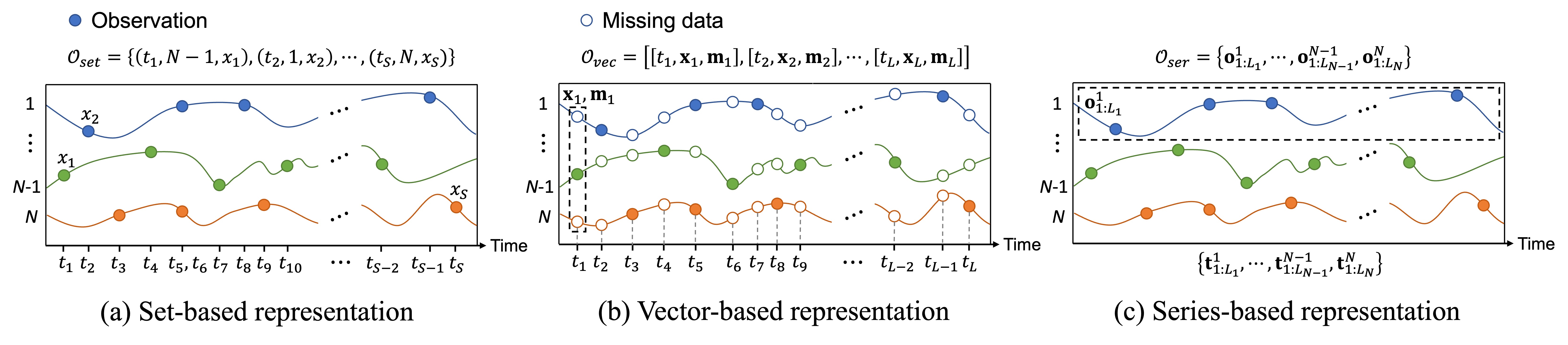
Figure 1. Diverse representation methods for irregularly sampled time series.

The modeling and analysis of ISTS differ fundamentally from those of RSTS due to the inherent irregularity and asynchrony among them (rubanova2019latent, ; zhang2021graph, ), which results in diverse representation methods of ISTS tailored to suit different models (che2018recurrent, ; horn2020set, ; shukla2020survey, ). These distinctive characteristics present the following significant challenges in fully harnessing the capabilities of PLMs for ISTS modeling and analysis: (1) Irregularity within ISTS. Unlike applying PLMs to process RSTS, the varying time intervals between adjacent observations within ISTS disrupt the consistent flow of the series data, making PLMs difficult to identify and capture the real temporal semantics and dependencies. For example, positional embeddings (radford2019language, ) in PLMs align well with the chronological order of RSTS, where observations occur at fixed intervals. However, it is unsuitable for ISTS as a fixed position might correspond to observations at varying times due to the irregularity of series, which results in inconsistent temporal semantics. (2) Asynchrony within ISTS. While considerable correlations often exist between time series of different variables, the observations within ISTS may be significantly misaligned due to irregular sampling or missing data (zhang2021graph, ; zhang2023irregular, ). This asynchrony complicates making direct comparisons and discerning correlations between the series, potentially obscuring or distorting the true relationships across variables (zhangirregular2024, ). Consequently, this poses a significant challenge in modeling correlations across different time series. (3) Diverse representation methods of ISTS. Unlike RSTS, usually represented as an orderly matrix of a series of vectors containing values from multiple variables, the representation methods of ISTS vary across different models. Unfortunately, our findings indicate that the commonly used set-based (horn2020set, ) and vector-based (che2018recurrent, ) representation methods by prior models largely hinder the powerful capabilities of PLMs for ISTS modeling due to their chaotic data landscape. This imposes a fundamental challenge in identifying a compatible representation method that can harness the full potential of PLMs for ISTS analysis.

To fully unleash the power of PLMs for ISTS analysis, this work introduces a series-based representation method, which is rarely used by previous works, to represent ISTS in a simple yet effective form. Building on this representation, we propose a unified PLM-based framework, ISTS-PLM, which incorporates time-aware and variable-aware PLMs tailored to address the challenging intra- and inter-time series modeling in ISTS. By further integrating a learnable input embedding layer and a task-specific output layer, ISTS-PLM is equipped to tackle diverse ISTS analytical tasks, such as classification, interpolation, and extrapolation.

Our major contributions are summarized as follows: (1) This is the first work to explore the potential of PLMs for ISTS analysis. We investigate the effects of various representation methods to maximize the efficacy of PLMs for ISTS. Our findings reveal that set-based and vector-based representations, commonly preferred in prior studies, constrain the performance of PLMs in analyzing ISTS. Consequently, we introduce a simple yet effective series-based representation to fully unleash its power for ISTS. (2) We propose a unified PLM-based framework that adapts two frozen PLMs, i.e., a time-aware PLM and a variable-aware PLM, with a learnable input embedding layer and a task-specific output layer to tackle diverse ISTS analytical tasks, addressing the significant challenges inherently existing in ISTS modeling. (3) Extensive experiments on a comprehensive benchmark demonstrate that ISTS-PLM consistently achieves state-of-the-art performance across all mainstream ISTS analytical tasks, including classification, interpolation, and extrapolation, as well as few-shot and zero-shot learning scenarios.

2. Related Works

2.1. Irregularly Sampled Time Series Analysis

The primary focus of existing research on ISTS analytical tasks includes classification, interpolation, and extrapolation. One straightforward method involves converting ISTS into a regularly sampled format with fixed time intervals (lipton2016directly, ), though this approach often results in significant information loss and missing data issues (shukla2020multi, ). Recent studies have shifted towards directly learning from ISTS. Specifically, some studies have enhanced RNNs by integrating a time gate (neil2016phased, ), a time decay term (che2018recurrent, ), or memory decomposition mechanism (baytas2017patient, ) to adapt the model’s memory updates for ISTS. Additionally, inspired by the Transformer’s success in processing linguistic sequences and visual data, numerous studies have sought to adapt the Transformer architecture and its attention mechanism for ISTS modeling (horn2020set, ; shukla2020multi, ; zhang2021graph, ; warpformer2023, ; li2023time, ; zhangirregular2024, ). Another line of studies involve employing neural Ordinary Differential Equations (ODEs) (chen2018neural, ) to capture the continuous dynamics and address the irregularities of ISTS (rubanova2019latent, ; de2019gru, ; bilovs2021neural, ; schirmer2022modeling, ). While these works offer a theoretically sound solution, their practical application is constrained by high computational costs associated with numerical integration (bilovs2021neural, ).

Although extensive efforts have been made on ISTS analysis, they primarily focus on addressing a limited range of analytical tasks, with a particular emphasis on classification. No previous works simultaneously address all mainstream tasks, i.e., classification, interpolation, and extrapolation, through a unified framework. Furthermore, despite PLMs having demonstrated transformative power in various research areas, such as NLP (min2023recent, ), graph learning (chen2024exploring, ), and even RSTS (jin2024position, ), their potential for ISTS remains under-explored.

2.2. Pre-Trained Language Models for Time Series

We have witnessed that a series of proactive studies explore adapting PLMs for time series analysis not only to enhance task performance but also to facilitate interdisciplinary, interpretative, and interactive analysis (jin2024position, ). These studies primarily fall into two categories: prompting-based and alignment-based methods. Prompting-based methods (xue2023promptcast, ; gruver2023large, ) treat numerical time series as textual data, using existing PLMs to process time series directly. However, the performance is not guaranteed due to the significant differences between time series and text modalities. Therefore, most recent works focus on alignment-based methods, aiming to align the encoded time series to the semantic space of PLMs, hence harnessing their powerful abilities of semantic pattern recognition and reasoning on processing time series. Specifically, model fine-tuning is an effective and the most widely used approach, involving directly tuning partial parameters of PLMs (zhou2023one, ; chang2023llm4ts, ; cao2023tempo, ; liu2024autotimes, ; chen2023gatgpt, ; liu2024spatial, ) or learning additional adapters (zhou2023one2, ). Moreover, model reprogramming (jin2024time, ; sun2023test, ) aims to directly encode the time series into text representation space that PLMs can understand, thus avoiding tuning PLMs’ parameters.

While significant efforts have been made to explore the potential of PLMs for RSTS, harnessing the power of PLMs for ISTS is much more challenging due to its characteristics of irregularity, asynchrony, and diverse representation methods, leaving it largely under-explored.

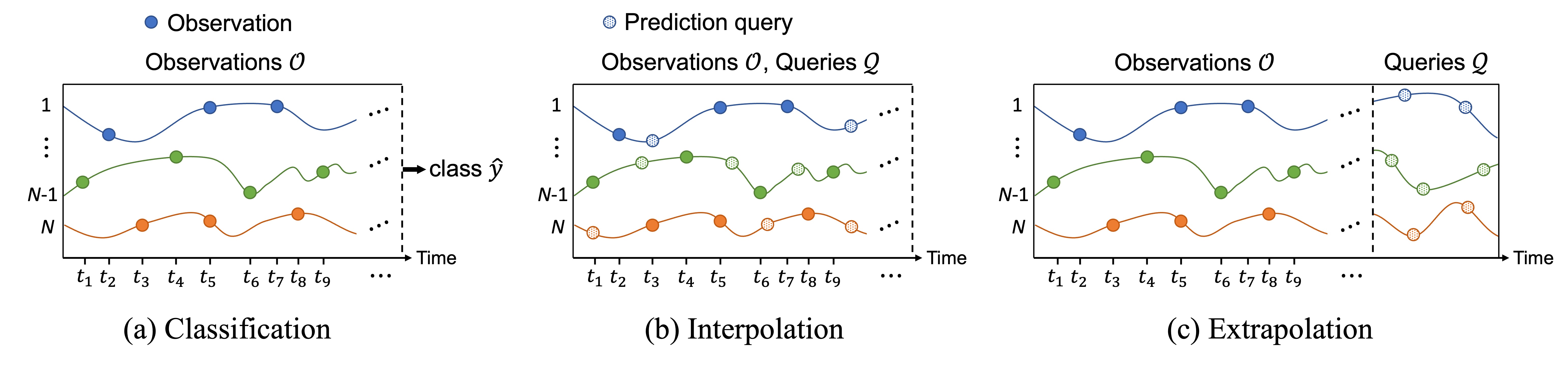
Figure 2. Mainstream analytical tasks for irregularly sampled time series.

3. Preliminary

3.1. Representation Methods for ISTS

Consider that an ISTS $\mathcal{O}$ has $N$ variables, each of which contains a series of observations that are irregularly sampled in varying time intervals. This ISTS can be represented by different methods as illustrated in Figure 1.

Set-Based Representation. Set-based representation method (horn2020set, ) views ISTS as a set of observation tuples $\mathcal{O}_{set}=\{(t_{s},n_{s},x_{s})\}_{s=1}^{S}$, where $t_{s}$ is the recorded time, $n_{s}$ indicates the variable of this observation, $x_{s}$ denotes the corresponding recorded value, and $S$ represents the total number of observations within the ISTS.

Vector-Based Representation. Vector-based representation method (che2018recurrent, ) has been commonly employed as a standard in current works (che2018recurrent, ; shukla2020multi, ; zhang2021graph, ; warpformer2023, ; baytas2017patient, ; rubanova2019latent, ; de2019gru, ; bilovs2021neural, ; schirmer2022modeling, ). This method represents ISTS using three matrix $\mathcal{O}_{vec}=(\mathcal{T},\mathcal{X},\mathcal{M})$. $\mathcal{T}=[t_{l}]_{l=1}^{L}\in\mathbb{R}^{L}$ represents the unique chronological timestamps of all observations across the ISTS. $\mathcal{X}={[[\tilde{x}^{n}_{l}]_{n=1}^{N}]_{l=1}^{L}}\in\mathbb{R}^{L\times N}$ records the values of variables at these timestamps, with $\tilde{x}^{n}_{l}$ representing the observed value of $n$-th variable at time $t_{l}$, or ‘NA’ if unobserved. $\mathcal{M}={[[m^{n}_{l}]_{n=1}^{N}]_{l=1}^{L}}\in\mathbb{R}^{L\times N}$ is a mask matrix indicating observation status, where $m^{n}_{l}=1$ signifies that $\tilde{x}^{n}_{l}$ is observed at time $t_{l}$, and zero otherwise. As a result, the ISTS is represented as a series of vectors $\mathcal{O}_{vec}=\left[t_{l},\mathbf{x}_{l},\mathbf{m}_{l}\right]_{l=1}^{L}=\left[t_{l},[\tilde{x}^{n}_{l}]_{n=1}^{N},[m^{n}_{l}]_{n=1}^{N}\right]_{l=1}^{L}\in\mathbb{R}^{L\times(2N+1)}$.

Series-Based Representation. Series-based representation me-thod represents the time series of each variable separately, and thus leads to $N$ univariant ISTS involving only real observations $\mathcal{O}_{ser}=\{\mathbf{o}^{n}_{1:L_{n}}\}_{n=1}^{N}=\{[(t_{i}^{n},x_{i}^{n})]_{i=1}^{L_{n}}\}_{n=1}^{N}$, where $L_{n}$ represents the number of real observations for $n$-th variable.

3.2. Problem Definitions

Figure 2 showcases the mainstream ISTS analytical tasks studied by existing research works, including classification, interpolation, and extrapolation.

Problem 1: ISTS Classification. Given ISTS observations $\mathcal{O}$, the classification problem is to infer a discrete class $\hat{y}$ (e.g., in-hospital mortality) for the ISTS: $\mathcal{F}\left(\mathcal{O}\right)\longrightarrow\hat{y},$ where $\mathcal{F}(\cdot)$ denotes the classification model we aim to learn.

Definition 1: Prediction Query. A prediction query is denoted as $(t,n)$, indicating a query to predict the recorded value $\hat{x}$ of variable $n$ at time $t$. The queried time may either fall within the observed time window for interpolation or extend beyond it for extrapolation.

Problem 2: ISTS Interpolation and Extrapolation. Given ISTS observations $\mathcal{O}$, and a set of ISTS prediction queries $\mathcal{Q}=\{(t_{j},n_{j})\}_{j=1}^{|\mathcal{Q}|}$, the problem is to predict recorded values $\hat{\mathcal{X}}=\{\hat{x}_{j}\}_{j=1}^{|\mathcal{Q}|}$ in correspondence to the prediction queries: $\mathcal{F}\left(\mathcal{O},\mathcal{Q}\right)\longrightarrow\hat{\mathcal{X}}.$

4. Methodology

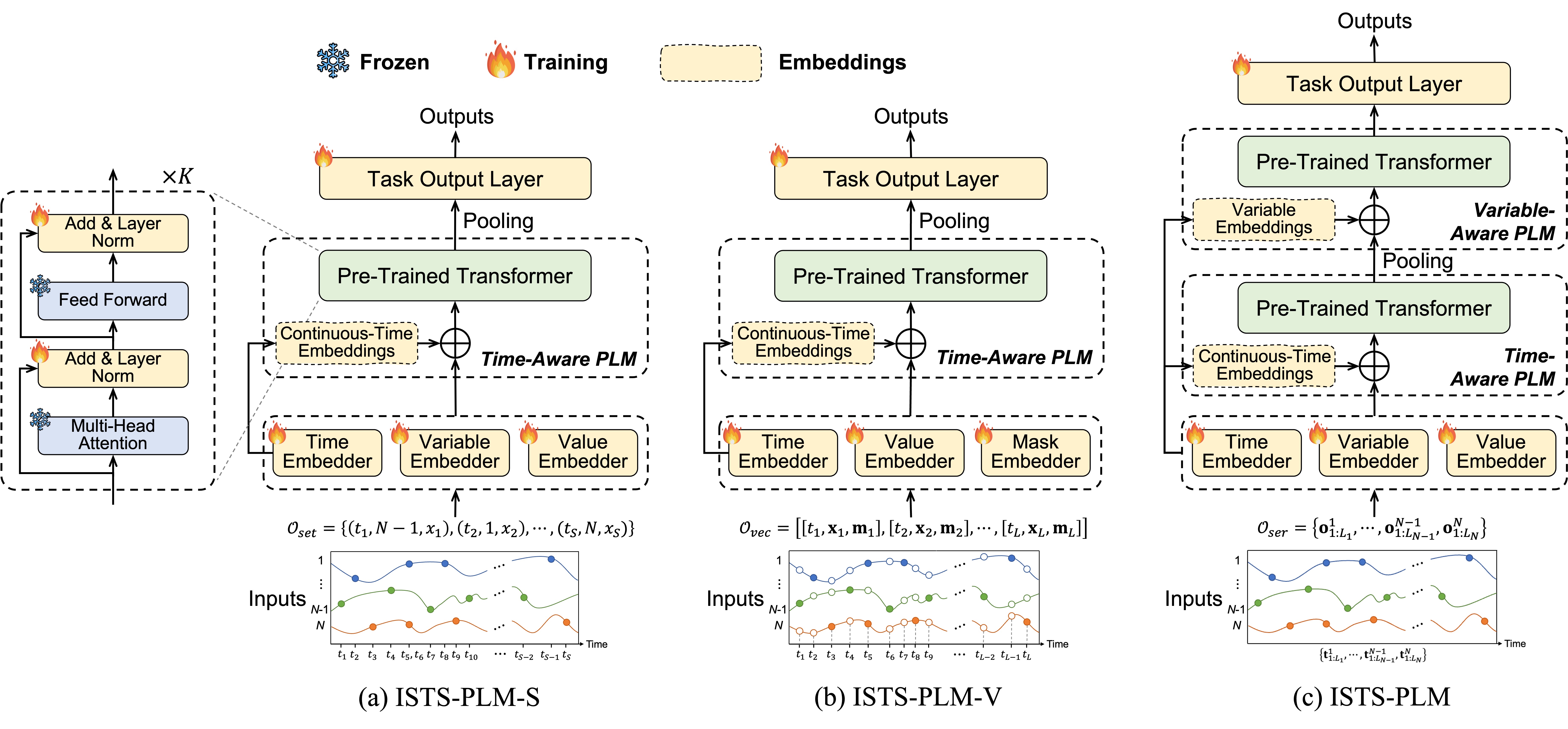
Figure 3. Framework overview of ISTS-PLM for set-based (ISTS-PLM-S), vector-based (ISTS-PLM-V), and series-based (ISTS-PLM) representation methods of ISTS. Given the representation outcome of an ISTS, we first embed it through a trainable input embedding layer to align the embedded ISTS to the semantic space of PLMs. Then the embedded series is fed to a time-aware PLM that replaces its positional embeddings with continuous-time embeddings to discern the irregular dynamics within ISTS. For series-based representation, we further introduce a variable-aware PLM to model variables’ correlations within the asynchronous ISTS. All the parameters of PLMs are frozen except layer normalization. Finally, we employ a trainable task output layer to project the output of PLM to address diverse ISTS tasks, such as classification, interpolation, and extrapolation.

The overview of ISTS-PLM is illustrated in Figure 3. We introduce PLMs, such as GPT (radford2019language, ) and BERT (kenton2019bert, ), for ISTS analysis. We investigate the effects of set-based, vector-based, and series-based representation methods of ISTS as the inputs for PLMs. The unified PLM-based framework, ISTS-PLM, encompasses a trainable input embedding layer, a trainable task output layer, and the PLM blocks. Inspired by (zhou2023one, ), we freeze all the parameters of the PLMs, except for fine-tuning a few parameters of the layer normalization. Nonetheless, we identify the following major differences from (zhou2023one, ): (1) We directly input the outcome series of different ISTS representation instead of patching them. (2) To better adapt PLM to model ISTS, we propose Time-Aware PLM by replacing its positional embeddings with learnable continuous-time embeddings, which empowers PLM to discern the irregular dynamics within ISTS. (3) For the modeling of series-based representation, we further present a variable-aware PLM that enables the model to understand and capture the correlations between variables within asynchronous multivariate ISTS.

4.1. Input Embedding

The input embedding layer aims to align the embedded ISTS to the semantic space of PLMs. Different ISTS representation methods may involve specific subsets of embedders, including time embedder, variable embedder, value embedder, and mask embedder.

Time Embedder. To incorporate meaningful temporal information into ISTS modeling, we introduce a time embedder (shukla2020multi, ) to encode the continuous-time within ISTS:

(1) $$\bm{t}[d]=\begin{cases}\omega_{0}\cdot t+\alpha_{0},&\text{ if }\quad d=0\\ \sin\left(\omega_{d}\cdot t+\alpha_{d}\right),&\text{ if }\quad 0<d<D\end{cases}$$

where the $\omega_{d}$ and $\alpha_{d}$ denote learnable parameters, with $D$ representing the dimension of continuous-time embedding. The linear term captures non-periodic patterns evolving over time, while the periodic terms account for periodicity within the time series, with $\omega_{d}$ and $\alpha_{d}$ indicating the frequency and phase of the sine function, respectively.

Variable Embedder. This embedder maps the variable $n$ into a $D$ dimensional embedding $\bm{n}$. This can be achieved by utilizing a learnable variable embedding lookup table $\mathbf{V}\in\mathbb{R}^{N\times D}$ and retrieving the corresponding embedding from the lookup table based on the variable indicator, or by using PLM to encode the descriptive text of variable, etc.

Value Embedder. We adopt a linear embedder layer to encode the recorded values into embeddings. For set-based and series-based representations, each recorded value is embedded by: $\bm{x}=x\mathbf{W}_{x}$, where $\mathbf{W}_{x}\in\mathbb{R}^{1\times D}$ is learnable mapping parameters. For vector-based representation, we encode the value vector at each time point into an integrated embedding: $\bm{x}_{l}=\mathbf{x}_{l}\mathbf{W}_{\mathbf{x}}$, where $\mathbf{W}_{\mathbf{x}}\in\mathbb{R}^{N\times D}$.

Mask Embedder. As vector-based representation additionally involves mask terms, we further encode the mask vectors into embeddings. Similar to value embedding, we utilize a linear embedder layer to obtain the mask embedding at each time point: $\bm{m}_{l}=\mathbf{m}_{l}\mathbf{W}_{m}$, where $\mathbf{W}_{m}\in\mathbb{R}^{N\times D}$ is learnable mapping parameters.

4.2. PLMs for ISTS Modeling

This section describes how we adapt PLM to model ISTS based on three representation methods, i.e., set-based, vector-based, and series-based representations.

4.2.1. PLM for Set-Based Representation.

Given a set of observation tuples $\mathcal{O}_{set}=\{t_{s},n_{s},x_{s}\}_{s=1}^{S}$, we first sort them in a chronological order. For each tuple, we integrate the embeddings of variable and value: $\bm{z}_{s}=\bm{n}_{s}+\bm{x}_{s}$, obtaining a series of embedded observations $\mathbf{Z}_{set}=\{\bm{z}_{s}\}_{s=1}^{S}\in\mathbb{R}^{S\times D}$, which is then inputted to PLM.

Due to the irregularity of time series, the same position in PLM might correspond to observations at varying recorded time with completely different temporal semantics. To empower PLM to seamlessly handle the irregular dynamics within ISTS, we present time-aware PLM that replaces the positional embeddings of PLM with continuous-time embedding derived from the time embedder. Consequently, the embedded observations will be seamlessly incorporated with temporal information: $\mathbf{Z}^{\prime}_{set}=\mathbf{Z}_{set}+\mathbf{TE}_{set}$, where $\mathbf{TE}_{set}=\{\bm{t}_{s}\}_{s=1}^{S}\in\mathbb{R}^{S\times D}$ are a series of embeddings of the continuous-times in correspondence to the input observations.

As the set size $S$ can vary across different ISTS, we summarize PLM’s outputs, $\mathbf{H}_{set}\in\mathbb{R}^{S\times D}$, into a fixed dimensional vector, $\mathbf{H}^{o}_{set}=pool(\mathbf{H}_{set})\in\mathbb{R}^{D}$, to facilitate the subsequent modeling and analysis, where $pool(\cdot)$ is a size-independent pooling function, such as average, maximum, and attention. We consistently use average pooling in our experiments for simplification.

4.2.2. PLM for Vector-Based Representation.

The vector-based representation observations $\mathcal{O}_{vec}$ are first embedded into $\mathbf{Z}_{vec}=\{\bm{z}_{l}\}_{l=1}^{L}\in\mathbb{R}^{L\times D}$, where $\bm{z}_{l}=\bm{x}_{l}+\bm{m}_{l}$. We do not involve variable embedding here because $\bm{z}_{l}$ represents an information integration of all variables at time $t_{l}$, and the value and mask embedders have been variable-aware during this integration. Likewise, $\mathbf{Z}_{vec}$ are subsequently processed by a time-aware PLM that seamlessly incorporates the inputs with temporal information, and the output $\mathbf{H}_{vec}\in\mathbb{R}^{L\times D}$ will be summarized into a fixed dimensional vector, $\mathbf{H}^{o}_{vec}=pool(\mathbf{H}_{vec})\in\mathbb{R}^{D}$, by a size-independent pooling function.

4.2.3. PLM for Series-Based Representation.

PLM for series-based representation includes the processes of intra-time series dependencies modeling and inter-time series correlations modeling.

Intra-Time Series Modeling. This involves modeling each univariant ISTS independently by using a time-aware PLM. Specifically, given $\mathcal{O}_{ser}=\{\mathbf{o}^{n}_{1:L_{n}}\}_{n=1}^{N}=\{[(t_{i}^{n},x_{i}^{n})]_{i=1}^{L_{n}}\}_{n=1}^{N}$, a series of observations of $n$-th variable is embedded to $\mathbf{x}^{n}_{1:L_{n}}=\{\bm{x}^{n}_{i}\}_{i=1}^{L_{n}}\in\mathbb{R}^{L_{n}\times D}$. To incorporate variable information, we prepend the variable embedding to the embedding series of each variable: $\mathbf{z}^{n}_{1:L_{n}+1}=[\bm{n},\mathbf{x}^{n}_{1:L_{n}}]$. This operation is akin to providing prompts to the inputs of a PLM, enabling it to discern which variable’s time series it is analyzing and thus stimulating its in-context learning capability (lester2021power, ). As a result, $\mathbf{z}^{n}_{1:L_{n}+1}$ is inputted to a time-aware PLM for intra-time series dependencies modeling. It initially incorporates continuous-time embeddings to the inputs: $\mathbf{z}^{n^{\prime}}_{1:L_{n}+1}=\mathbf{z}^{n}_{1:L_{n}+1}+\mathbf{TE}^{n}_{ser}$, where $\mathbf{TE}^{n}_{ser}=\left[\bm{0},[\bm{t}^{n}_{i}]_{i=1}^{L_{n}}\right]$ and $\bm{0}$ represents an all-zero vector. This PLM then processes the inputs through its pre-trained transformer blocks and outputs a series of hidden vectors $\mathbf{h}^{n}_{1:L_{n}+1}\in\mathbb{R}^{(L_{n}+1)\times D}$.

Inter-Time Series Modeling. The time series of different variables usually display notable correlations that insights from other variables may offer valuable information and significantly enhance the analysis of each variable (zhang2021graph, ; zhangirregular2024, ). However, the hidden vectors $\{\mathbf{h}^{n}_{1:L_{n}+1}\}_{n=1}^{N}$ of different variables obtained from the aforementioned intra-time series modeling can be significantly misaligned at times due to their irregularly sampled series, presenting the asynchrony challenge in modeling inter-time series correlations. To address this, we similarly summarize the series of hidden vectors into a fixed dimensional vector via the pooling operation: $\mathbf{h}^{n}_{ser}=pool(\mathbf{h}^{n}_{1:L_{n}+1})\in\mathbb{R}^{D}$, and thus different ISTS will be aligned in a global view. Once ${\mathbf{H}}_{ser}=\{\mathbf{h}^{n}_{ser}\}_{n=1}^{N}\in\mathbb{R}^{N\times D}$ obtained, we employ another variable-aware PLM, which replaces its positional embeddings with the trained variable embeddings: $\mathbf{H}^{\prime}_{ser}={\mathbf{H}}_{ser}+\mathbf{VE}_{ser}$, where $\mathbf{VE}_{ser}=\{\bm{n}\}_{n=1}^{N}$. It facilitates the understanding of variable-specific characteristics and aligns with the position-invariant nature of the variables, thereby enhancing the modeling of inter-time series correlations. The resulting output produced by this variable-aware PLM is represented as $\mathbf{H}^{o}_{ser}=\{\mathbf{h}^{o,n}_{ser}\}_{n=1}^{N}\in\mathbb{R}^{N\times D}$.

4.3. Task Output Projection

The task output layer aims to project the output of PLMs to address different ISTS tasks, such as classification, interpolation, and extrapolation.

Classification. A linear classification layer processes the resulting output of PLMs to infer a class for the ISTS: $\hat{y}=\operatorname{Softmax}(\mathbf{H}^{o}_{\cdot}\mathbf{W}_{c}+\mathbf{b}_{c})\in\mathbb{R}^{C}$, where $C$ is the number of classes, $\mathbf{W}_{c}$ and $\mathbf{b}_{c}\in\mathbb{R}^{C}$ are learnable parameters, and $\mathbf{W}_{c}\in\mathbb{R}^{D\times C}$ for the outputs of set-based and vector-based representations, $\mathbf{W}_{c}\in\mathbb{R}^{ND\times C}$ for the flattened output of series-based representation. The entire learnable parameters of ISTS classification model are learned by optimizing a cross-entropy loss between the inferred class and ground truth label.

Interpolation and Extrapolation. The output projection of interpolation and extrapolation varies slightly across these representation methods. For set-based and vector-based methods, given the resulting output $\mathbf{H}^{o}_{\cdot}$ of the ISTS and a prediction query $(t,n)$, a prediction layer instantiated by a Multi-Layer Perception (MLP) is used to generate the predicted values at time $t$: $\hat{x}=\operatorname{MLP}([\mathbf{H}^{o}_{\cdot}\|t])[n]$.

For series-based method, we directly utilize the output $\mathbf{h}^{o,n}_{ser}\in\mathbb{R}^{D}$ of the corresponding variable $n$ to predict its value through a shared prediction layer: $\hat{x}=\operatorname{MLP}([\mathbf{h}^{o,n}_{ser}\|t])$.

The prediction model is trained by minimizing the Mean Squared Error (MSE) loss between the prediction and the ground truth: $\mathcal{L}_{p}=\frac{1}{N}\sum_{n=1}^{N}\frac{1}{Q_{n}}\sum_{j=1}^{Q_{n}}\left(\hat{x}^{n}_{j}-x^{n}_{j}\right)^{2},$ where $Q_{n}$ represents the total number of prediction queries in correspondence to $n$-th variable.

5. Experiments

Table 1. Overall performance comparison on irregularly sampled time series Classification task. Bold represents the best-performing results and underline indicates the second-best results. ISTS-PLM-S, ISTS-PLM-V, ISTS-PLM denote our model with set-based, vector-based, and series-based ISTS representations, respectively.

	P12		P19		PAM
Method	AUROC	AUPRC	AUROC	AUPRC	Accuracy	Precision	Recall	F1 score
Transformer	$83.3{\scriptstyle\,\pm\,0.7}$	$47.9{\scriptstyle\,\pm\,3.6}$	$80.7{\scriptstyle\,\pm\,3.8}$	$42.7{\scriptstyle\,\pm\,7.7}$	$83.5{\scriptstyle\,\pm\,1.5}$	$84.8{\scriptstyle\,\pm\,1.5}$	$86.0{\scriptstyle\,\pm\,1.2}$	$85.0{\scriptstyle\,\pm\,1.3}$
MTGNN	$74.4{\scriptstyle\,\pm\,6.7}$	$35.5{\scriptstyle\,\pm\,6.0}$	$81.9{\scriptstyle\,\pm\,6.2}$	$39.9{\scriptstyle\,\pm\,8.9}$	$83.4{\scriptstyle\,\pm\,1.9}$	$85.2{\scriptstyle\,\pm\,1.7}$	$86.1{\scriptstyle\,\pm\,1.9}$	$85.9{\scriptstyle\,\pm\,2.4}$
DGM2-O	$84.4{\scriptstyle\,\pm\,1.6}$	$47.3{\scriptstyle\,\pm\,3.6}$	$86.7{\scriptstyle\,\pm\,3.4}$	$44.7{\scriptstyle\,\pm\,11.7}$	$82.4{\scriptstyle\,\pm\,2.3}$	$85.2{\scriptstyle\,\pm\,1.2}$	$83.9{\scriptstyle\,\pm\,2.3}$	$84.3{\scriptstyle\,\pm\,1.8}$
IP-Net	$82.6{\scriptstyle\,\pm\,1.4}$	$47.6{\scriptstyle\,\pm\,3.1}$	$84.6{\scriptstyle\,\pm\,1.3}$	$38.1{\scriptstyle\,\pm\,3.7}$	$74.3{\scriptstyle\,\pm\,3.8}$	$75.6{\scriptstyle\,\pm\,2.1}$	$77.9{\scriptstyle\,\pm\,2.2}$	$76.6{\scriptstyle\,\pm\,2.8}$
GRU-D	$81.9{\scriptstyle\,\pm\,2.1}$	$46.1{\scriptstyle\,\pm\,4.7}$	$83.9{\scriptstyle\,\pm\,1.7}$	$46.9{\scriptstyle\,\pm\,2.1}$	$83.3{\scriptstyle\,\pm\,1.6}$	$84.6{\scriptstyle\,\pm\,1.2}$	$85.2{\scriptstyle\,\pm\,1.6}$	$84.8{\scriptstyle\,\pm\,1.2}$
SeFT	$73.9{\scriptstyle\,\pm\,2.5}$	$31.1{\scriptstyle\,\pm\,4.1}$	$81.2{\scriptstyle\,\pm\,2.3}$	$41.9{\scriptstyle\,\pm\,3.1}$	$67.1{\scriptstyle\,\pm\,2.2}$	$70.0{\scriptstyle\,\pm\,2.4}$	$68.2{\scriptstyle\,\pm\,1.5}$	$68.5{\scriptstyle\,\pm\,1.8}$
mTAND	$84.2{\scriptstyle\,\pm\,0.8}$	$48.2{\scriptstyle\,\pm\,3.4}$	$84.4{\scriptstyle\,\pm\,1.3}$	$50.6{\scriptstyle\,\pm\,2.0}$	$92.9{\scriptstyle\,\pm\,0.8}$	$93.8{\scriptstyle\,\pm\,0.8}$	$94.0{\scriptstyle\,\pm\,0.9}$	$93.8{\scriptstyle\,\pm\,0.8}$
Raindrop	$82.8{\scriptstyle\,\pm\,1.7}$	$44.0{\scriptstyle\,\pm\,3.0}$	$87.0{\scriptstyle\,\pm\,2.3}$	$51.8{\scriptstyle\,\pm\,5.5}$	$88.5{\scriptstyle\,\pm\,1.5}$	$89.9{\scriptstyle\,\pm\,1.5}$	$89.9{\scriptstyle\,\pm\,0.6}$	$89.8{\scriptstyle\,\pm\,1.0}$
Warpformer	$\underline{86.6}{\scriptstyle\,\pm\,0.8}$	$\underline{55.5}{\scriptstyle\,\pm\,3.5}$	$88.1{\scriptstyle\,\pm\,2.5}$	$\underline{56.1}{\scriptstyle\,\pm\,4.4}$	$95.1{\scriptstyle\,\pm\,0.8}$	$95.7{\scriptstyle\,\pm\,0.8}$	$95.7{\scriptstyle\,\pm\,0.9}$	$95.7{\scriptstyle\,\pm\,0.8}$
FPT	$84.8{\scriptstyle\,\pm\,1.1}$	$50.7{\scriptstyle\,\pm\,3.0}$	$87.3{\scriptstyle\,\pm\,2.9}$	$51.6{\scriptstyle\,\pm\,3.6}$	$94.0{\scriptstyle\,\pm\,1.4}$	$95.3{\scriptstyle\,\pm\,0.9}$	$94.7{\scriptstyle\,\pm\,1.1}$	$94.9{\scriptstyle\,\pm\,1.1}$
Time-LLM	$84.4{\scriptstyle\,\pm\,1.8}$	$50.2{\scriptstyle\,\pm\,1.6}$	$85.1{\scriptstyle\,\pm\,2.6}$	$50.1{\scriptstyle\,\pm\,3.4}$	$93.4{\scriptstyle\,\pm\,1.2}$	$94.2{\scriptstyle\,\pm\,1.3}$	$94.7{\scriptstyle\,\pm\,1.0}$	$94.4{\scriptstyle\,\pm\,1.1}$
ViTST	$85.1{\scriptstyle\,\pm\,0.8}$	$51.1{\scriptstyle\,\pm\,4.1}$	$\underline{89.2}{\scriptstyle\,\pm\,2.0}$	$53.1{\scriptstyle\,\pm\,3.4}$	$\underline{95.8}{\scriptstyle\,\pm\,1.3}$	$\underline{96.2}{\scriptstyle\,\pm\,1.3}$	$\underline{96.1}{\scriptstyle\,\pm\,1.1}$	$\underline{96.5}{\scriptstyle\,\pm\,1.2}$
ISTS-PLM-S	$85.8{\scriptstyle\,\pm\,0.9}$	$52.1{\scriptstyle\,\pm\,4.5}$	$88.1{\scriptstyle\,\pm\,1.4}$	$51.8{\scriptstyle\,\pm\,2.2}$	$89.6{\scriptstyle\,\pm\,0.7}$	$89.6{\scriptstyle\,\pm\,0.7}$	$91.9{\scriptstyle\,\pm\,1.4}$	$90.4{\scriptstyle\,\pm\,0.9}$
ISTS-PLM-V	$85.9{\scriptstyle\,\pm\,1.4}$	$52.2{\scriptstyle\,\pm\,3.7}$	$87.5{\scriptstyle\,\pm\,2.4}$	$53.1{\scriptstyle\,\pm\,4.0}$	$94.3{\scriptstyle\,\pm\,1.3}$	$94.5{\scriptstyle\,\pm\,1.4}$	$95.2{\scriptstyle\,\pm\,1.4}$	$94.8{\scriptstyle\,\pm\,1.3}$
ISTS-PLM	$\mathbf{87.6}{\scriptstyle\,\pm\,1.4}$	$\mathbf{57.6}{\scriptstyle\,\pm\,3.3}$	$\mathbf{89.4}{\scriptstyle\,\pm\,2.2}$	$\mathbf{56.9}{\scriptstyle\,\pm\,5.0}$	$\mathbf{96.3}{\scriptstyle\,\pm\,0.5}$	$\mathbf{96.9}{\scriptstyle\,\pm\,1.0}$	$\mathbf{96.8}{\scriptstyle\,\pm\,0.4}$	$\mathbf{96.8}{\scriptstyle\,\pm\,0.7}$

Table 2. Overall performance comparison on irregularly sampled time series Interpolation and Extrapolation tasks. Bold represents the best-performing results and underline indicates the second-best results.

		PhysioNet		MIMIC		Human Activity
Task	Method	MSE$\times 10^{-3}$	MAE$\times 10^{-2}$	MSE$\times 10^{-2}$	MAE$\times 10^{-2}$	MSE$\times 10^{-3}$	MAE$\times 10^{-2}$
Interpolation	GRU-D	$6.18{\scriptstyle\,\pm\,0.23}$	$4.35{\scriptstyle\,\pm\,0.06}$	$2.06{\scriptstyle\,\pm\,0.05}$	$7.83{\scriptstyle\,\pm\,0.14}$	$2.74{\scriptstyle\,\pm\,0.09}$	$3.40{\scriptstyle\,\pm\,0.08}$
	SeFT	$9.46{\scriptstyle\,\pm\,0.12}$	$5.51{\scriptstyle\,\pm\,0.12}$	$2.12{\scriptstyle\,\pm\,0.02}$	$8.08{\scriptstyle\,\pm\,0.11}$	$14.95{\scriptstyle\,\pm\,0.03}$	$9.42{\scriptstyle\,\pm\,0.02}$
	Raindrop	$10.65{\scriptstyle\,\pm\,0.12}$	$5.80{\scriptstyle\,\pm\,0.07}$	$2.31{\scriptstyle\,\pm\,0.04}$	$8.62{\scriptstyle\,\pm\,0.10}$	$15.21{\scriptstyle\,\pm\,0.12}$	$9.51{\scriptstyle\,\pm\,0.05}$
	Warpformer	$6.37{\scriptstyle\,\pm\,0.34}$	$4.43{\scriptstyle\,\pm\,0.20}$	$1.93{\scriptstyle\,\pm\,0.06}$	$7.57{\scriptstyle\,\pm\,0.12}$	$2.59{\scriptstyle\,\pm\,0.15}$	$3.20{\scriptstyle\,\pm\,0.11}$
	mTAND	$5.65{\scriptstyle\,\pm\,0.08}$	$4.18{\scriptstyle\,\pm\,0.07}$	$1.93{\scriptstyle\,\pm\,0.05}$	$7.49{\scriptstyle\,\pm\,0.08}$	$2.07{\scriptstyle\,\pm\,0.17}$	$2.74{\scriptstyle\,\pm\,0.23}$
	Latent-ODE	$6.84{\scriptstyle\,\pm\,0.34}$	$4.67{\scriptstyle\,\pm\,0.14}$	$1.89{\scriptstyle\,\pm\,0.08}$	$7.67{\scriptstyle\,\pm\,0.47}$	$3.12{\scriptstyle\,\pm\,0.22}$	$3.76{\scriptstyle\,\pm\,0.16}$
	Neural Flow	$6.77{\scriptstyle\,\pm\,0.06}$	$4.60{\scriptstyle\,\pm\,0.07}$	$2.18{\scriptstyle\,\pm\,0.11}$	$8.30{\scriptstyle\,\pm\,0.28}$	$3.73{\scriptstyle\,\pm\,0.06}$	$4.20{\scriptstyle\,\pm\,0.05}$
	CRU	$10.30{\scriptstyle\,\pm\,0.10}$	$5.47{\scriptstyle\,\pm\,0.05}$	$2.52{\scriptstyle\,\pm\,0.04}$	$8.87{\scriptstyle\,\pm\,0.03}$	$7.17{\scriptstyle\,\pm\,0.32}$	$6.35{\scriptstyle\,\pm\,0.14}$
	t-PatchGNN	$\underline{4.75}{\scriptstyle\,\pm\,0.03}$	$\underline{3.59}{\scriptstyle\,\pm\,0.03}$	$\underline{1.55}{\scriptstyle\,\pm\,0.08}$	$\underline{6.25}{\scriptstyle\,\pm\,0.21}$	$\underline{1.95}{\scriptstyle\,\pm\,0.12}$	$\underline{2.54}{\scriptstyle\,\pm\,0.14}$
	FPT	$12.24{\scriptstyle\,\pm\,0.07}$	$5.77{\scriptstyle\,\pm\,0.12}$	$3.71{\scriptstyle\,\pm\,0.01}$	$10.76{\scriptstyle\,\pm\,0.09}$	$2.85{\scriptstyle\,\pm\,0.09}$	$3.26{\scriptstyle\,\pm\,0.08}$
	Time-LLM	$12.43{\scriptstyle\,\pm\,0.08}$	$6.00{\scriptstyle\,\pm\,0.12}$	$3.63{\scriptstyle\,\pm\,0.05}$	$10.39{\scriptstyle\,\pm\,0.14}$	$2.92{\scriptstyle\,\pm\,0.01}$	$3.34{\scriptstyle\,\pm\,0.03}$
	ISTS-PLM-S	$7.74{\scriptstyle\,\pm\,0.35}$	$5.02{\scriptstyle\,\pm\,0.16}$	$2.00{\scriptstyle\,\pm\,0.03}$	$7.71{\scriptstyle\,\pm\,0.08}$	$4.27{\scriptstyle\,\pm\,0.79}$	$4.63{\scriptstyle\,\pm\,0.53}$
	ISTS-PLM-V	$7.12{\scriptstyle\,\pm\,0.30}$	$4.58{\scriptstyle\,\pm\,0.08}$	$1.90{\scriptstyle\,\pm\,0.04}$	$7.50{\scriptstyle\,\pm\,0.10}$	$3.03{\scriptstyle\,\pm\,0.22}$	$3.70{\scriptstyle\,\pm\,0.22}$
	ISTS-PLM	$\mathbf{4.55}{\scriptstyle\,\pm\,0.08}$	$\mathbf{3.37}{\scriptstyle\,\pm\,0.02}$	$\mathbf{1.47}{\scriptstyle\,\pm\,0.01}$	$\mathbf{5.94}{\scriptstyle\,\pm\,0.01}$	$\mathbf{1.93}{\scriptstyle\,\pm\,0.01}$	$\mathbf{2.52}{\scriptstyle\,\pm\,0.01}$
Extrapolation	PatchTST	$12.00{\scriptstyle\,\pm\,0.23}$	$6.02{\scriptstyle\,\pm\,0.14}$	$3.78{\scriptstyle\,\pm\,0.03}$	$12.43{\scriptstyle\,\pm\,0.10}$	$4.29{\scriptstyle\,\pm\,0.14}$	$4.80{\scriptstyle\,\pm\,0.09}$
	MTGNN	$6.26{\scriptstyle\,\pm\,0.18}$	$4.46{\scriptstyle\,\pm\,0.07}$	$2.71{\scriptstyle\,\pm\,0.23}$	$9.55{\scriptstyle\,\pm\,0.65}$	$3.03{\scriptstyle\,\pm\,0.03}$	$3.53{\scriptstyle\,\pm\,0.03}$
	GRU-D	$5.59{\scriptstyle\,\pm\,0.09}$	$4.08{\scriptstyle\,\pm\,0.05}$	$1.76{\scriptstyle\,\pm\,0.03}$	$7.53{\scriptstyle\,\pm\,0.09}$	$2.94{\scriptstyle\,\pm\,0.05}$	$3.53{\scriptstyle\,\pm\,0.06}$
	SeFT	$9.22{\scriptstyle\,\pm\,0.18}$	$5.40{\scriptstyle\,\pm\,0.08}$	$1.87{\scriptstyle\,\pm\,0.01}$	$7.84{\scriptstyle\,\pm\,0.08}$	$12.20{\scriptstyle\,\pm\,0.17}$	$8.43{\scriptstyle\,\pm\,0.07}$
	Raindrop	$9.82{\scriptstyle\,\pm\,0.08}$	$5.57{\scriptstyle\,\pm\,0.06}$	$1.99{\scriptstyle\,\pm\,0.03}$	$8.27{\scriptstyle\,\pm\,0.07}$	$14.92{\scriptstyle\,\pm\,0.14}$	$9.45{\scriptstyle\,\pm\,0.05}$
	Warpformer	$5.94{\scriptstyle\,\pm\,0.35}$	$4.21{\scriptstyle\,\pm\,0.12}$	$1.73{\scriptstyle\,\pm\,0.04}$	$7.58{\scriptstyle\,\pm\,0.13}$	$2.79{\scriptstyle\,\pm\,0.04}$	$3.39{\scriptstyle\,\pm\,0.03}$
	mTAND	$6.23{\scriptstyle\,\pm\,0.24}$	$4.51{\scriptstyle\,\pm\,0.17}$	$1.85{\scriptstyle\,\pm\,0.06}$	$7.73{\scriptstyle\,\pm\,0.13}$	$3.22{\scriptstyle\,\pm\,0.07}$	$3.81{\scriptstyle\,\pm\,0.07}$
	Latent-ODE	$6.05{\scriptstyle\,\pm\,0.57}$	$4.23{\scriptstyle\,\pm\,0.17}$	$1.89{\scriptstyle\,\pm\,0.19}$	$8.11{\scriptstyle\,\pm\,0.52}$	$3.34{\scriptstyle\,\pm\,0.11}$	$3.94{\scriptstyle\,\pm\,0.12}$
	Neural Flow	$7.20{\scriptstyle\,\pm\,0.07}$	$4.67{\scriptstyle\,\pm\,0.04}$	$1.87{\scriptstyle\,\pm\,0.05}$	$8.03{\scriptstyle\,\pm\,0.19}$	$4.05{\scriptstyle\,\pm\,0.13}$	$4.46{\scriptstyle\,\pm\,0.09}$
	CRU	$8.56{\scriptstyle\,\pm\,0.26}$	$5.16{\scriptstyle\,\pm\,0.09}$	$1.97{\scriptstyle\,\pm\,0.02}$	$7.93{\scriptstyle\,\pm\,0.19}$	$6.97{\scriptstyle\,\pm\,0.78}$	$6.30{\scriptstyle\,\pm\,0.47}$
	t-PatchGNN	$\underline{4.98}{\scriptstyle\,\pm\,0.08}$	$\underline{3.72}{\scriptstyle\,\pm\,0.03}$	$\underline{1.69}{\scriptstyle\,\pm\,0.03}$	$\underline{7.22}{\scriptstyle\,\pm\,0.09}$	$\underline{2.66}{\scriptstyle\,\pm\,0.03}$	$\underline{3.15}{\scriptstyle\,\pm\,0.02}$
	FPT	$10.95{\scriptstyle\,\pm\,0.02}$	$5.37{\scriptstyle\,\pm\,0.02}$	$4.00{\scriptstyle\,\pm\,0.03}$	$12.34{\scriptstyle\,\pm\,0.11}$	$3.03{\scriptstyle\,\pm\,0.09}$	$3.36{\scriptstyle\,\pm\,0.10}$
	Time-LLM	$11.56{\scriptstyle\,\pm\,0.19}$	$5.80{\scriptstyle\,\pm\,0.25}$	$4.41{\scriptstyle\,\pm\,0.01}$	$13.43{\scriptstyle\,\pm\,0.03}$	$3.21{\scriptstyle\,\pm\,0.01}$	$3.53{\scriptstyle\,\pm\,0.02}$
	ISTS-PLM-S	$7.62{\scriptstyle\,\pm\,0.20}$	$4.84{\scriptstyle\,\pm\,0.06}$	$1.82{\scriptstyle\,\pm\,0.05}$	$7.78{\scriptstyle\,\pm\,0.07}$	$5.02{\scriptstyle\,\pm\,1.02}$	$5.08{\scriptstyle\,\pm\,0.63}$
	ISTS-PLM-V	$6.71{\scriptstyle\,\pm\,0.26}$	$4.52{\scriptstyle\,\pm\,0.11}$	$1.79{\scriptstyle\,\pm\,0.02}$	$7.60{\scriptstyle\,\pm\,0.06}$	$3.46{\scriptstyle\,\pm\,0.16}$	$4.01{\scriptstyle\,\pm\,0.14}$
	ISTS-PLM	$\mathbf{4.92}{\scriptstyle\,\pm\,0.05}$	$\mathbf{3.65}{\scriptstyle\,\pm\,0.04}$	$\mathbf{1.64}{\scriptstyle\,\pm\,0.02}$	$\mathbf{7.02}{\scriptstyle\,\pm\,0.14}$	$\mathbf{2.58}{\scriptstyle\,\pm\,0.03}$	$\mathbf{3.12}{\scriptstyle\,\pm\,0.04}$

5.1. Experimental Setup

To demonstrate the effectiveness of ISTS-PLM, we conduct extensive experiments across mainstream ISTS analytical tasks, including classification, interpolation, and extrapolation. More experiments studying the effect of different PLM’s layers, PLMs composition, training & inference cost are provided in A.1, A.2, A.3 in Appendix.

5.1.1. Datasets

For ISTS classification task, we refer to previous works (li2023time, ; zhang2021graph, ) that introduce healthcare datasets P12 (physionet, ), P19 (reyna2019early, ) and biomechanics dataset PAM (reiss2012introducing, ) for a thorough evaluation. We follow the experimental settings of P12, P19, and PAM from ViTST (li2023time, ), where each dataset is randomly partitioned into training, validation, and test sets with 8:1:1 proportion. Each experiment is performed with five different data partitions and reports the mean and standard deviation of results. The indices of these partitions are kept consistent across all methods compared.

For ISTS interpolation and extrapolation tasks, referring to t-PatchGNN (zhangirregular2024, ), we utilize three natural ISTS datasets: PhysioNet, MIMIC, and Human Activity (misc_localization_data_for_person_activity_196, ), from the domains of healthcare and biomechanics. Consistently, we randomly divide all the ISTS samples within each dataset into training, validation, and test sets, maintaining a proportional split of 6:2:2, and adopt the min-max normalization to normalize the original observation values. To mitigate randomness, we run each experiment with five different random seeds and report the mean and standard deviation of the results. More details of these datasets are provided in Appendix A.4.

5.1.2. Metrics

For classification task, following prior research (li2023time, ; zhang2021graph, ), we utilize Area Under the Receiver Operating Characteristic Curve (AUROC) and Area Under the Precision-Recall Curve (AUPRC) for the performance evaluation of imbalanced datasets P12 and P19, and use Accuracy, Precision, Recall, and F1 score to evaluate balanced dataset PAM. Higher is better for all the above metrics.

Referring to previous work (zhangirregular2024, ), we introduce both Mean Square Error (MSE) and Mean Absolute Error (MAE) to evaluate the prediction performance for interpolation and extrapolation tasks. Lower is better for MSE and MAE.

Table 3. Model ablation results on Classification task. Bold represents the best-performing results.

	P12		P19		PAM
Method	AUROC	AUPRC	AUROC	AUPRC	Accuracy	Precision	Recall	F1 score
ISTS-PLM	$\mathbf{87.6}{\scriptstyle\,\pm\,1.4}$	$\mathbf{57.6}{\scriptstyle\,\pm\,3.3}$	$\mathbf{89.4}{\scriptstyle\,\pm\,2.2}$	$\mathbf{56.9}{\scriptstyle\,\pm\,5.0}$	$\mathbf{96.3}{\scriptstyle\,\pm\,0.5}$	$96.9{\scriptstyle\,\pm\,1.0}$	$\mathbf{96.8}{\scriptstyle\,\pm\,0.4}$	$\mathbf{96.8}{\scriptstyle\,\pm\,0.7}$
rp Transformer	$86.7{\scriptstyle\,\pm\,1.0}$	$54.6{\scriptstyle\,\pm\,3.3}$	$86.3{\scriptstyle\,\pm\,2.1}$	$47.4{\scriptstyle\,\pm\,3.2}$	$94.6{\scriptstyle\,\pm\,0.6}$	$95.5{\scriptstyle\,\pm\,0.5}$	$95.3{\scriptstyle\,\pm\,0.7}$	$95.3{\scriptstyle\,\pm\,0.5}$
w/o TA-PLM	$86.4{\scriptstyle\,\pm\,1.0}$	$54.4{\scriptstyle\,\pm\,4.1}$	$89.1{\scriptstyle\,\pm\,2.4}$	$54.2{\scriptstyle\,\pm\,4.1}$	$95.0{\scriptstyle\,\pm\,0.6}$	$95.7{\scriptstyle\,\pm\,0.5}$	$95.7{\scriptstyle\,\pm\,0.5}$	$95.6{\scriptstyle\,\pm\,0.5}$
w/o VA-PLM	$87.0{\scriptstyle\,\pm\,1.2}$	$55.4{\scriptstyle\,\pm\,2.9}$	$87.6{\scriptstyle\,\pm\,2.7}$	$51.5{\scriptstyle\,\pm\,4.1}$	$91.5{\scriptstyle\,\pm\,1.9}$	$92.4{\scriptstyle\,\pm\,2.3}$	$93.1{\scriptstyle\,\pm\,1.5}$	$92.3{\scriptstyle\,\pm\,2.4}$
w/o TE	$87.2{\scriptstyle\,\pm\,0.9}$	$57.2{\scriptstyle\,\pm\,3.5}$	$88.3{\scriptstyle\,\pm\,2.6}$	$53.3{\scriptstyle\,\pm\,3.4}$	$96.1{\scriptstyle\,\pm\,0.4}$	$\mathbf{97.0}{\scriptstyle\,\pm\,0.4}$	$96.4{\scriptstyle\,\pm\,0.6}$	$96.6{\scriptstyle\,\pm\,0.3}$
w/o VE	$\mathbf{87.6}{\scriptstyle\,\pm\,1.6}$	$57.2{\scriptstyle\,\pm\,3.6}$	$88.6{\scriptstyle\,\pm\,2.3}$	$55.4{\scriptstyle\,\pm\,4.0}$	$95.5{\scriptstyle\,\pm\,1.3}$	$96.2{\scriptstyle\,\pm\,1.3}$	$96.0{\scriptstyle\,\pm\,0.6}$	$96.1{\scriptstyle\,\pm\,1.0}$

5.1.3. Baselines

To evaluate the performance in ISTS classification task, we incorporate the following baseline models for a fair comparison, including vanilla Transformer (vaswani2017attention, ); (sparse) multivariate time series analysis models: MTGNN (wu2020connecting, ), DGM²-O (wu2021dynamic, ); ISTS classification models: IP-Net (shukla2018interpolation, ), GRU-D (che2018recurrent, ), SeFT (horn2020set, ), mTAND (shukla2020multi, ), Raindrop (zhang2021graph, ), Warpformer (warpformer2023, ), and pre-trained vision transformers-based model ViTST (li2023time, ); as well as PLM-based models designed for RSTS analysis: FPT (zhou2023one, ), Time-LLM (jin2024time, ). All these models are trained for 20 epochs, and the model’s parameters achieving the highest AUROC on the validation set are selected for testing (zhang2021graph, ; li2023time, ).

For ISTS interpolation and extrapolation tasks, except adapting the representative baselines above to these two tasks, we further incorporate several models tailored for the ISTS prediction tasks, including Latent-ODE (rubanova2019latent, ), Neural Flow (bilovs2021neural, ), CRU (schirmer2022modeling, ), and t-PatchGNN (zhangirregular2024, ). For both tasks, early stopping is applied to all models if the validation loss doesn’t decrease over 10 epochs. More details of these baselines are provided in Appendix A.5.

5.1.4. Implementation Details

While most of the experiments are conducted on a Linux server with a 20-core Intel(R) Xeon(R) Platinum 8255C CPU @ 2.50GHz and an NVIDIA Tesla V100 GPU, the interpolation and extrapolation experiments of PhysioNet and MIMIC datasets are performed on a 8-core Intel(R) Xeon(R) Platinum 8358P CPU @ 2.60GHz and an NVIDIA A800 GPU. We use the first 6 layers (out of 12) of GPT-2 (124M) as time-aware PLM and the first 6 layers (out of 12) of BERT (110M) as variable-aware PLM in ISTS-PLM for classification tasks and Human Activity’s interpolation and extrapolation. The tasks on PhysioNet and MIMIC are using the first 3 layers of PLMs. The embedding dimension $D$ is 768. We freeze all parameters of the PLMs, except for fine-tuning only a few parameters of the layer normalization. For simplification, we learn a variable embedding lookup table as the variable embedder. The model is trained using the Adam optimizer with a learning rate $1\times 10^{-3}$ for classification and $5\times 10^{-4}$ for the other tasks. ISTS-PLM employs consistent dataset splitting and validation strategies as the baseline models to ensure fair comparison.

Table 4. Few-shot learning task on 10% data. Bold represents the best-performing results.

	P12		P19		PAM
Method	AUROC	AUPRC	AUROC	AUPRC	Accuracy	Precision	Recall	F1 score
GRU-D	$79.5{\scriptstyle\,\pm\,2.0}$	$44.8{\scriptstyle\,\pm\,3.3}$	$83.3{\scriptstyle\,\pm\,3.0}$	$33.0{\scriptstyle\,\pm\,3.2}$	$79.2{\scriptstyle\,\pm\,2.3}$	$81.4{\scriptstyle\,\pm\,2.5}$	$80.6{\scriptstyle\,\pm\,1.3}$	$80.5{\scriptstyle\,\pm\,1.4}$
mTAND	$80.4{\scriptstyle\,\pm\,1.4}$	$45.2{\scriptstyle\,\pm\,3.5}$	$76.7{\scriptstyle\,\pm\,1.2}$	$25.7{\scriptstyle\,\pm\,2.8}$	$78.7{\scriptstyle\,\pm\,1.6}$	$81.1{\scriptstyle\,\pm\,0.8}$	$81.1{\scriptstyle\,\pm\,2.1}$	$80.6{\scriptstyle\,\pm\,1.4}$
Raindrop	$72.9{\scriptstyle\,\pm\,3.3}$	$31.6{\scriptstyle\,\pm\,4.9}$	$75.5{\scriptstyle\,\pm\,3.9}$	$41.3{\scriptstyle\,\pm\,4.7}$	$65.6{\scriptstyle\,\pm\,4.1}$	$69.7{\scriptstyle\,\pm\,6.1}$	$65.3{\scriptstyle\,\pm\,5.6}$	$65.2{\scriptstyle\,\pm\,6.1}$
Warpformer	$82.2{\scriptstyle\,\pm\,1.3}$	$45.4{\scriptstyle\,\pm\,3.1}$	$84.0{\scriptstyle\,\pm\,2.0}$	$43.7{\scriptstyle\,\pm\,3.8}$	$84.0{\scriptstyle\,\pm\,1.2}$	$85.3{\scriptstyle\,\pm\,1.8}$	$86.4{\scriptstyle\,\pm\,1.6}$	$85.6{\scriptstyle\,\pm\,1.3}$
FPT	$79.3{\scriptstyle\,\pm\,0.8}$	$41.6{\scriptstyle\,\pm\,2.6}$	$81.2{\scriptstyle\,\pm\,2.1}$	$44.3{\scriptstyle\,\pm\,4.1}$	$84.2{\scriptstyle\,\pm\,3.0}$	$86.3{\scriptstyle\,\pm\,2.3}$	$86.4{\scriptstyle\,\pm\,2.6}$	$85.9{\scriptstyle\,\pm\,2.7}$
Time-LLM	$79.3{\scriptstyle\,\pm\,2.7}$	$39.8{\scriptstyle\,\pm\,3.5}$	$82.6{\scriptstyle\,\pm\,2.7}$	$39.5{\scriptstyle\,\pm\,4.4}$	$83.4{\scriptstyle\,\pm\,1.7}$	$84.5{\scriptstyle\,\pm\,1.3}$	$84.5{\scriptstyle\,\pm\,2.0}$	$85.0{\scriptstyle\,\pm\,1.5}$
ViTST	$69.6{\scriptstyle\,\pm\,2.1}$	$29.5{\scriptstyle\,\pm\,2.3}$	$71.3{\scriptstyle\,\pm\,1.6}$	$33.2{\scriptstyle\,\pm\,1.4}$	$80.3{\scriptstyle\,\pm\,3.2}$	$85.1{\scriptstyle\,\pm\,2.1}$	$81.8{\scriptstyle\,\pm\,3.2}$	$82.6{\scriptstyle\,\pm\,3.3}$
ISTS-PLM	$\mathbf{83.8}{\scriptstyle\,\pm\,1.7}$	$\mathbf{49.6}{\scriptstyle\,\pm\,3.9}$	$\mathbf{85.3}{\scriptstyle\,\pm\,2.2}$	$\mathbf{45.9}{\scriptstyle\,\pm\,5.0}$	$\mathbf{85.7}{\scriptstyle\,\pm\,1.3}$	$\mathbf{87.8}{\scriptstyle\,\pm\,1.0}$	$\mathbf{87.7}{\scriptstyle\,\pm\,1.6}$	$\mathbf{87.5}{\scriptstyle\,\pm\,1.1}$

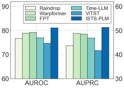
(a) Adaptation by ICUType

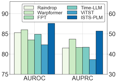
(b) Adaptation by Age

Figure 4. Performance comparison of zero-shot adaptation.

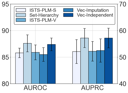
(a) Classification on P12

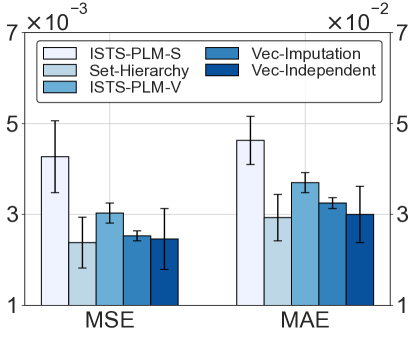
(b) Interpolation on Human Activity

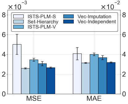
(c) Extrapolation on Human Activity

Figure 5. Results of the variants of ISTS-PLM with set-based and vector-based representations.

5.2. Main Results

Table 1 and Table 2 present the performance comparison for ISTS classification, interpolation and extrapolation tasks. Our ISTS-PLM (using series-based representation) consistently outperforms all other baselines, including the state-of-the-art (SOTA) cross-domain adaptation-based methods: FPT, Time-LLM, and ViTST, across all tasks and datasets, demonstrating ISTS-PLM’s universal superiority for ISTS analysis. However, it is non-trivial to obtain this level of performance. We observe that ISTS-PLM with typical set-based (ISTS-PLM-S) and vector-based (ISTS-PLM-V) representations often yield sub-optimal results. They perform even worse on interpolation and extrapolation tasks, which require each variable to be more meticulously and distinctly analyzed. We provide further analysis on different ISTS representations of our model in Section 5.5.

Additionally, although we utilize the same series-based representation of ISTS as inputs for the PLM-based models: FPT and Time-LLM, our ISTS-PLM significantly outperforms them across all ISTS tasks. This demonstrates the effectiveness of time-aware and variable-aware PLMs tailored for intra- and inter-series modeling within ISTS.

5.3. Ablation Study

We evaluate the performance of ISTS-PLM and its five variants. (1) ISTS-PLM represents the complete model without any ablation; (2) rp Transformer replaces PLMs with trainable transformers; (3) w/o TA-PLM removes Time-Aware PLM; (4) w/o VA-PLM removes Variable-Aware PLM; (5) w/o TE removes continuous-time embeddings and directly fine-tunes the original positional embeddings in PLM; (6) w/o VE removes variable embeddings and directly fine-tunes the original positional embeddings in PLM.

The ablation results are provided in Table 3 and Table 5. As can be seen, replacing PLMs with trainable transformers consistently leads to remarkable performance degradation across all tasks and datasets, underscoring the critical role of PLMs in enhancing ISTS analysis. Additionally, we find removing VA-PLM generally results in a larger performance decrease in classification task, while removing TA-PLM and continuous-time embeddings overall leads to a more substantial performance drop in interpolation and forecasting tasks. This might be attributed to classification being a higher-level task that requires greater attention to the relationships and summaries among all variables, whereas interpolation and forecasting typically need more precise modeling of each variable’s observations and their temporal flow. However, this is not absolute in the case of MIMIC. This might be because MIMIC has a large number of variables but very sparse observations, making inter-series modeling more important than intra-series modeling. Furthermore, we observe that using variable embedding in place of the original positional embeddings of PLM generally leads to better performance. This is because variables are position-invariant and possess inherent semantic characteristics, while positional embeddings are sequential and lack variable-related semantics, necessitating additional effort in fine-tuning extra parameters to adapt them appropriately.

5.4. Few-shot and Zero-shot Learning

As existing ISTS works primarily focus on classification tasks, we conduct few-shot and zero-shot learning experiments on classification datasets. For each dataset, we randomly select 10% of the training set to assess the model’s few-shot learning ability. Table 4 presents the model comparison in few-shot learning scenario, where ISTS-PLM consistently outperforms the other SOTA baselines. Notably, while ViTST, another cross-domain adaptation-based model for ISTS, suffers a significant performance drop, our model maintains a much more robust performance, likely due to its need to learn far fewer parameters than ViTST, as reported in Table 7.

To evaluate the model’s zero-shot adaptation ability, we divide the samples (i.e., patients) in P12 dataset into multiple disjoint groups based on individual attributes, including ICUType (Coronary Care Unit, Cardiac Surgery Recovery Unit, Surgical ICU, Medical ICU) and Age (Old (¿=65), Young (¡65)). This division ensures marked diversity between groups. The model is trained on some groups and tested on others. For ICUType, we select patients belonging to Medical ICU as the test set and the others as training data. For Age, we select Young patients as the test set and Old patients as training data. The results in Figure 4 showcase that ISTS-PLM consistently outperforms other SOTA baselines, demonstrating its robust cross-group zero-shot adaptation ability.

5.5. Analysis on Distinct Representation Methods

This section provides a further analysis of the key failure reasons for ISTS-PLM when using set-based and vector-based representations. We explore several variants of ISTS-PLM-S and ISTS-PLM-V. For set-based representation, we examine (1) Set-Hierarchy: observations are processed by PLMs in a hierarchical way, i.e., first independently modeling the observation series of each variable, then modeling the correlations between these variables. This makes it equivalent to the series-based representation. For vector-based representation, we examine (2) Vec-Independent: each variable’s time series is first processed independently by the PLM, followed by PLM-based inter-variable modeling; (3) Vec-Imputation: missing values in the representation are imputed using a forward-filling strategy.

Figure 5 displays the results of these variants across three ISTS analytical tasks. The findings suggest that the strategy of first modeling each variable’s series independently, followed by modeling their correlations, significantly enhances the performance of PLMs in processing ISTS. Unlike ISTS-PLM-S, which models all observed tuples in a mixed time-variable manner, or ISTS-PLM-V, which mixes all variables’ observations at each time point, this approach organizes ISTS in a more structured and cleaner manner, and mitigates interference and noise from other variables, thereby simplifying the learning task for PLM. It transforms ISTS modeling into a two-stage sequence modeling problem, i.e., intra- and inter-series modeling, more effectively harnessing the powerful capabilities of PLMs for sequence semantic recognition and understanding.

6. Conclusion

This paper explored the potential of Pre-trained Language Models (PLMs) for Irregularly Sampled Time Series (ISTS) analysis and presented a unified PLM-based framework, ISTS-PLM, to address various ISTS analytical tasks. We investigated three methods for representing ISTS and identified a simple yet effective series-based representation to maximize the efficacy of PLMs for ISTS modeling and analysis. We conducted comprehensive experiments on six datasets spanning scientific domains of healthcare and biomechanics. The results demonstrated that ISTS-PLM, incorporating a time-aware PLM and a variable-aware PLM with only fine-tuning their layer normalization parameters along with a trainable input embedding layer and a task output layer, could consistently achieve state-of-the-art performance across various mainstream ISTS analytical tasks, such as classification, interpolation, and extrapolation, as well as few-shot and zero-shot scenarios compared to seventeen competitive baseline models.

Appendix A Additional Experiments

Table 5. Model ablation results on Interpolation and Extrapolation tasks. Bold represents the best-performing results.

		PhysioNet		MIMIC		Human Activity
Task	Method	MSE$\times 10^{-3}$	MAE$\times 10^{-2}$	MSE$\times 10^{-2}$	MAE$\times 10^{-2}$	MSE$\times 10^{-3}$	MAE$\times 10^{-2}$
Interpolation	ISTS-PLM	$\mathbf{4.55}{\scriptstyle\,\pm\,0.08}$	$\mathbf{3.37}{\scriptstyle\,\pm\,0.02}$	$\mathbf{1.47}{\scriptstyle\,\pm\,0.01}$	$\mathbf{5.94}{\scriptstyle\,\pm\,0.01}$	$\mathbf{1.93}{\scriptstyle\,\pm\,0.01}$	$\mathbf{2.52}{\scriptstyle\,\pm\,0.01}$
	rp Transformer	$4.71{\scriptstyle\,\pm\,0.13}$	$3.46{\scriptstyle\,\pm\,0.08}$	$2.10{\scriptstyle\,\pm\,0.08}$	$6.68{\scriptstyle\,\pm\,0.21}$	$2.91{\scriptstyle\,\pm\,0.04}$	$3.32{\scriptstyle\,\pm\,0.06}$
	w/o TA-PLM	$5.47{\scriptstyle\,\pm\,0.18}$	$3.78{\scriptstyle\,\pm\,0.08}$	$1.49{\scriptstyle\,\pm\,0.02}$	$6.05{\scriptstyle\,\pm\,0.08}$	$2.85{\scriptstyle\,\pm\,0.01}$	$3.29{\scriptstyle\,\pm\,0.01}$
	w/o VA-PLM	$4.94{\scriptstyle\,\pm\,0.13}$	$3.52{\scriptstyle\,\pm\,0.10}$	$1.88{\scriptstyle\,\pm\,0.04}$	$7.48{\scriptstyle\,\pm\,0.15}$	$2.53{\scriptstyle\,\pm\,0.54}$	$3.02{\scriptstyle\,\pm\,0.44}$
	w/o TE	$4.85{\scriptstyle\,\pm\,0.11}$	$3.52{\scriptstyle\,\pm\,0.11}$	$\mathbf{1.47}{\scriptstyle\,\pm\,0.01}$	$5.98{\scriptstyle\,\pm\,0.07}$	$2.25{\scriptstyle\,\pm\,0.07}$	$2.90{\scriptstyle\,\pm\,0.08}$
	w/o VE	$4.67{\scriptstyle\,\pm\,0.24}$	$3.44{\scriptstyle\,\pm\,0.09}$	$1.50{\scriptstyle\,\pm\,0.01}$	$5.93{\scriptstyle\,\pm\,0.12}$	$2.38{\scriptstyle\,\pm\,0.56}$	$2.93{\scriptstyle\,\pm\,0.51}$
Extrapolation	ISTS-PLM	$\mathbf{4.92}{\scriptstyle\,\pm\,0.05}$	$\mathbf{3.65}{\scriptstyle\,\pm\,0.04}$	$\mathbf{1.64}{\scriptstyle\,\pm\,0.02}$	$7.02{\scriptstyle\,\pm\,0.14}$	$\mathbf{2.58}{\scriptstyle\,\pm\,0.03}$	$\mathbf{3.12}{\scriptstyle\,\pm\,0.04}$
	rp Transformer	$5.18{\scriptstyle\,\pm\,0.16}$	$3.78{\scriptstyle\,\pm\,0.09}$	$2.63{\scriptstyle\,\pm\,0.15}$	$8.49{\scriptstyle\,\pm\,0.09}$	$2.81{\scriptstyle\,\pm\,0.06}$	$3.22{\scriptstyle\,\pm\,0.06}$
	w/o TA-PLM	$5.94{\scriptstyle\,\pm\,0.23}$	$4.02{\scriptstyle\,\pm\,0.10}$	$1.70{\scriptstyle\,\pm\,0.06}$	$7.24{\scriptstyle\,\pm\,0.21}$	$3.92{\scriptstyle\,\pm\,0.33}$	$4.13{\scriptstyle\,\pm\,0.20}$
	w/o VA-PLM	$4.99{\scriptstyle\,\pm\,0.05}$	$3.68{\scriptstyle\,\pm\,0.04}$	$1.92{\scriptstyle\,\pm\,0.07}$	$8.09{\scriptstyle\,\pm\,0.20}$	$2.87{\scriptstyle\,\pm\,0.18}$	$3.25{\scriptstyle\,\pm\,0.12}$
	w/o TE	$5.04{\scriptstyle\,\pm\,0.13}$	$3.74{\scriptstyle\,\pm\,0.05}$	$1.65{\scriptstyle\,\pm\,0.02}$	$\mathbf{6.94}{\scriptstyle\,\pm\,0.06}$	$2.83{\scriptstyle\,\pm\,0.09}$	$3.41{\scriptstyle\,\pm\,0.09}$
	w/o VE	$4.94{\scriptstyle\,\pm\,0.20}$	$3.68{\scriptstyle\,\pm\,0.15}$	$1.66{\scriptstyle\,\pm\,0.01}$	$7.02{\scriptstyle\,\pm\,0.09}$	$2.59{\scriptstyle\,\pm\,0.06}$	$3.14{\scriptstyle\,\pm\,0.05}$

A.1. Parameter Sensitivity

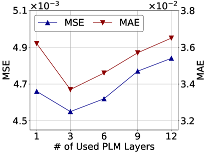
(a) PhysioNet

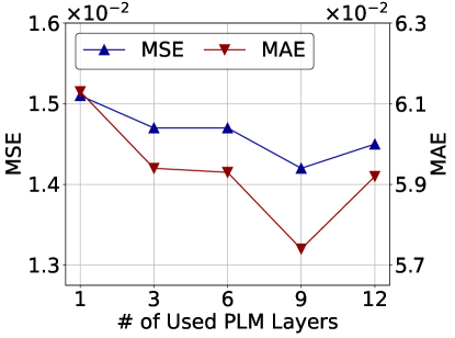
(b) MIMIC

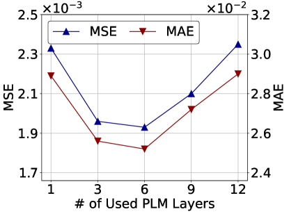
(c) Human Activity

Figure 6. Effect of different number of used layers in PLMs.

Taking the interpolation task as a representative, we study the effect of using different numbers of PLMs’ layers on various datasets. As shown in Figure 6, the optimal configuration for PLM’s layer can vary across datasets. However, using too less (i.e., 1) or too many (i.e., 12) PLM’s layers usually results in poorer performance. This is because too few layers may fail to capture the necessary complexity and dependencies within ISTS, while too many layers can complicate the process of adaptation and optimization, increasing the risk of overfitting.

A.2. Effect of Distinct PLMs

Table 6. Effect of distinct PLMs composition for ISTS-PLM.

	PhysioNet		MIMIC		Human Activity
Composition	MSE$\times 10^{-3}$	MAE$\times 10^{-2}$	MSE$\times 10^{-2}$	MAE$\times 10^{-2}$	MSE$\times 10^{-3}$	MAE$\times 10^{-2}$
GPT-Bert	$\mathbf{4.55}{\scriptstyle\,\pm\,0.08}$	$\mathbf{3.37}{\scriptstyle\,\pm\,0.02}$	$1.47{\scriptstyle\,\pm\,0.01}$	$5.94{\scriptstyle\,\pm\,0.01}$	$\mathbf{1.93}{\scriptstyle\,\pm\,0.01}$	$\mathbf{2.52}{\scriptstyle\,\pm\,0.01}$
GPT-GPT	$4.79{\scriptstyle\,\pm\,0.13}$	$3.46{\scriptstyle\,\pm\,0.03}$	$1.54{\scriptstyle\,\pm\,0.01}$	$6.17{\scriptstyle\,\pm\,0.17}$	$2.05{\scriptstyle\,\pm\,0.08}$	$2.64{\scriptstyle\,\pm\,0.08}$
Bert-Bert	$4.75{\scriptstyle\,\pm\,0.03}$	$3.56{\scriptstyle\,\pm\,0.04}$	$\mathbf{1.45}{\scriptstyle\,\pm\,0.01}$	$\mathbf{5.86}{\scriptstyle\,\pm\,0.08}$	$1.94{\scriptstyle\,\pm\,0.01}$	$\mathbf{2.52}{\scriptstyle\,\pm\,0.01}$
Bert-GPT	$4.76{\scriptstyle\,\pm\,0.14}$	$3.53{\scriptstyle\,\pm\,0.11}$	$1.56{\scriptstyle\,\pm\,0.01}$	$6.27{\scriptstyle\,\pm\,0.11}$	$2.91{\scriptstyle\,\pm\,0.09}$	$3.35{\scriptstyle\,\pm\,0.14}$

Table 6 presents the results of different PLMs backbone composition for our model’s time-aware PLM and variable-aware PLM modelus on interpolation task. The results indicate that using GPT for intra-series modeling and Bert for inter-series modeling achieves the best overall performance. This might be attributed to GPT’s causal masking pre-training strategy and unidirectional, autoregressive properties, making it effective in modeling sequences where the order of data points is important, such as intra-time series dependencies. In contrast, BERT’s bidirectional and contextual understanding, derived from pre-training to consider both preceding and succeeding contexts, allows it to capture complex interactions between multiple variables more effectively.

A.3. Training & Inference Cost

Table 7. Comparison on training & inference costs of classification on P12.

Model	Training parameters	Training time per step (s)	Inference time per sample (s)
GRU-D (64)	29K	0.257	0.045
mTAND (64)	345K	0.134	0.010
Raindrop (160)	452K	0.211	0.077
Warpformer (64)	146K	0.143	0.017
GRU-D (768)	2M	0.258	0.046
mTAND (768)	20M	0.306	0.069
Raindrop (772)	11M	1.102	0.966
Warpformer (768)	16M	0.163	0.021
ViTST (768)	202M	2.151	0.417
ISTS-PLM (768)	127K	0.232	0.043

This test is performed on a Linux server with a 20-core Intel(R) Xeon(R) Platinum 8255C CPU @ 2.50GHz and an NVIDIA Tesla V100 GPU. Table 7 presents a comparison of training parameters, training time per update step, and inference time per sample for the classification task on P12. ISTS-PLM achieves a comparable training and inference efficiency to the recommended hidden dimensions of state-of-the-art (SOTA) baselines. Notably, when these models are standardized to the same hidden dimension of 768, ISTS-PLM outperforms most of the baseline models in both training and inference efficiency. Additionally, ISTS-PLM requires fewer training parameters compared to most of these baselines.

A.4. Dataset Details

Table 8. Statistics of used irregularly sampled time series datasets for classification, interpolation and extrapolation tasks. ‘Imbalanced’ denotes the classes of samples are imbalanced. ‘Missing ratio’ refers to the proportion of missing observations relative to the total number of possible observations in a fully observed dataset.

Datasets	#Samples	#Variables	#Classes	Imbalanced	Missing ratio
P12	11,988	34	2	True	$88.4\%$
P19	38,803	36	2	True	$94.9\%$
PAM	5,333	17	8	False	$60.0\%$
PhysioNet	12,000	41	-	-	$85.7\%$
MIMIC	23,457	96	-	-	$96.7\%$
Human Activity	5,400	12	-	-	$75.0\%$

Table 8 provides the statistics of the used datasets P12, P19, PAM for ISTS classification, and PhysioNet, MIMIC, Human Activity for interpolation and extrapolation.

P12/PhysioNet: PhysioNet Mortality Prediction Challenge 2012. The P12/PhysioNet dataset [16] comprises clinical data from 11,988/12,000 ICU patients (P12 excluding 12 inappropriate samples). For each patient, the dataset includes 36 irregularly sampled sensor observations and 5 static demographic features collected during the first 48 hours of their ICU stay. The objective of classification is to predict patient mortality, a binary classification task, with negative samples constituting approximately 7% of the total. For the interpolation task, we randomly mask 30% timestamps’ observations within ISTS and aim to reconstruct them based on unmasked observed data. For the extrapolation task, we follow t-PatchGNN [42] to utilize the initial 24 hours as observed data to predict the queried values for the subsequent 24 hours.

P19: PhysioNet Sepsis Early Prediction Challenge 2019. The P19 dataset [28] comprises clinical data from 38,803 patients, aiming to predict the onset of sepsis (a binary label) within the next 6 hours. Each patient is monitored using 34 irregularly sampled sensors, including 8 vital signs and 26 laboratory values, alongside 6 demographic features. This binary classification task is highly imbalanced, with only around 4% positive samples.

PAM: PAMAP2 Physical Activity Monitoring. The PAM dataset [27] includes data from 9 subjects performing 18 physical activities, each subject wearing 3 inertial measurement units. Following previous works [44, 20], for irregular time series classification, we excluded the ninth subject due to the short duration of their sensor readouts. The continuous signals were segmented into windows of 600 time steps with a 50% overlap. Out of the original 18 activities, 10 were excluded due to having fewer than 500 samples, leaving 8 activities for classification, resulting in an 8-way classification task. The final dataset comprises 5,333 samples, each containing 600 continuous observations. To simulate irregular time series, 60% of the observations were randomly removed. No static features are provided and 8 categories are approximately balanced.

MIMIC: Medical Information Mart for Intensive Care. MIMIC [1] is a comprehensive and publicly available clinical database that includes electronic health records in critical care. This dataset contains 23,457 ISTS samples for different patients, covering the first 48 hours following their admission, and each patient comprises 96 variables. For the interpolation task, we randomly mask 30% timestamps’ observations within ISTS and reconstruct them using the unmasked observed data. For the extrapolation task, we follow t-PatchGNN [42] to employ the initial 24-hour period as the observed data to predict target values for subsequent 24 hours.

Human Activity: Localization Data for Person Activity. Human Activity [36] encompasses 12 variables derived from irregularly measured 3D positional data collected by four sensors positioned on the human left ankle, right ankle, belt, and chest. This dataset is derived from observations of five individuals engaged in a diverse array of activities, including walking, sitting, lying down, standing, and others. To better suit realistic prediction scenarios, we chunk the original time series into 5,400 ISTS samples, each spanning 4,000 milliseconds. For the interpolation task, we randomly mask 30% timestamps’ observations within ISTS and reconstruct them using the unmasked observed data. For the extrapolation task, we follow t-PatchGNN [42] to utilize the initial 3,000 milliseconds as observed data to predict the positional values of sensors in the subsequent 1,000 milliseconds.

A.5. Baseline Details

We incorporate seventeen baselines into our experiments for a fair comparison. The settings and results of classification and extrapolation tasks entirely refer to ViTST [20] and t-PatchGNN [42], respectively. In terms of the interpolation task, we meticulously tune the key hyperparameters of the baseline models around their recommended settings. We standardize the hidden dimensions to 64 for Physionet and MIMIC, and to 32 for Human Activity. Training is conducted using the Adam optimizer, with early stopping applied if the validation loss does not decrease after 10 epochs. To adapt the ISTS analysis baseline models to the interpolation task, we replace their original output layer with the interpolation prediction layer instantiated by a three-layer MLP.

As the setups of most baselines for classification and extrapolation have been detailed in ViTST [20] and t-PatchGNN [42], respectively, we mainly provide their settings for interpolation.

GRU-D [6] is a GRU-based model designed to address irregularly sampled time series by incorporating time decay and missing data imputation strategies. We set learning rate to $1\times 10^{-3}$ and use the implementation provided at https://github.com/zhiyongc/GRU-D.

SeFT [15] transforms time series into a set encoding and utilizes set functions to model them. In our experiment, we configure it with 2 layers and a learning rate of $1\times 10^{-3}$. We use the implementation provided by https://github.com/mims-harvard/Raindrop.

Raindrop [44] employs graph neural networks and temporal self-attention to capture dependencies between sensors, adaptively estimating unaligned observations based on neighboring measurements. In our experiment, we configure it with an observation dimension of 4 and 2 layers with 2 heads for the Transformer. The learning rate is set to $1\times 10^{-3}$. We use the official implementation provided at https://github.com/mims-harvard/Raindrop.

Warpformer [41] is a SOTA Transformer-based model designed for ISTS classification. It features a warping module for ISTS synchronization at a predefined scale and a custom attention module for enhanced representation learning. In our experiment, we set the warp number to 0-0.2-1, with 1 head and 3 layers for classification, and 2 layers for interpolation. The learning rate is set to $1\times 10^{-3}$. We utilized the official implementation available at https://github.com/imJiawen/Warpformer.

mTAND [32] is a model for ISTS classification and interpolation, which learns embeddings for numerical values tied to continuous time steps and derives fixed-length representations for variable-length sequential data using an attention mechanism. In our experiments, we set k-iwae to 5, std to 0.01, the number of reference points to 64, and the learning rate to $1\times 10^{-3}$. We use the official implementation provided at https://github.com/reml-lab/mTAN.

Latent-ODE [29] is an ODE-based model that enhances RNNs by incorporating continuous-time hidden state dynamics specified by neural ODEs. In our experiment, we configure it with 3 rec-layers and gen-layers for PhysioNet, and 1 for MIMIC and Human Activity. The learning rate is set to $1\times 10^{-3}$. We use the official implementation provided at https://github.com/YuliaRubanova/latent-ode.

Neural Flow [3] models the ODEs’ solution curves using neural networks. For the MIMIC dataset, we set 4 flow layers, 2 hidden layers, a rec-dim of 20, and use a GRU flow model with a TimeTanh time-net. The activation function is ReLU. For other datasets, we configure 2 flow layers, 3 hidden layers, a rec-dim of 40, and employ a coupling flow model with a TimeLinear time-net. The activation function is Tanh. The time-hidden-dim is 8 and the learning rate is $1\times 10^{-3}$ across all datasets. We use the official implementation provided at https://github.com/mbilos/neural-flows-experiments.

CRU [30] integrates the Kalman Filter with an encoder-decoder architecture to enable latent state updates in ODEs. In our experiment, we configure the timestamp scaling factor for numerical stability to 0.3 for Human Activity and 0.2 for other datasets. The encoder uses a squared variance activation function, while the decoder employs an exponential one. The transition net’s activation function is ReLU. We set the number of biases to 15 for Human Activity and 20 for others, with a bandwidth of 3 for Human Activity and 10 for others. The learning rate is $1\times 10^{-3}$. We use the official implementation provided at https://github.com/boschresearch-/Continuous-Recurrent-Units.

t-PatchGNN [42] is a SOTA model for ISTS extrapolation. It presents a transformable patching approach for converting univariate irregular time series into temporally-aligned patches of variable lengths, followed by time-adaptive graph neural networks to capture the dynamic inter-series correlations within ISTS. For our interpolation task, the patch window size for PhysioNet and MIMIC is set to 8 hours, and 300 milliseconds for Human Activity. The learning rate is $1\times 10^{-3}$. We use the official implementation provided at https://github.com/usail-hkust/t-PatchGNN/.

FPT [47] introduces a frozen PLM to address RSTS analytical tasks. In our experiment, we use the following settings: the representation method of input is the same as ISTS-PLM (i.e., series-based). To adapt the representation of ISTS, the patch size is set to 48 and the stride length is 24. The number of used layers for the PLM is 6. The activation function for the output is geLU. The learning rate is $5\times 10^{-4}$. We use the official implementation provided at https://github.com/DAMO-DI-ML/NeurIPS2023-One-Fits-All.

Time-LLM [17] propose a framework to reprogram an existing LLM to perform RSTS forecasting. In our experiment, we use the following settings: the representation method of input is the same as ISTS-PLM (i.e., series-based). The size of the patch is 48 and the length of the stride is 24 to adapt the representation of ISTS. The learning rate is $1\times 10^{-4}$. We use the official implementation provided at https://github.com/KimMeen/Time-LLM.

References

- (1) L. Shen H. L. Li-Wei M. Feng M. Ghassemi B. Moody P. Szolovits L. A. Celi A. Johnson, T. Pollard and R. G. Mark. Mimic-iii, a freely accessible critical care database. Scientific data, 3(1):1–9, 2016.
- (2) Inci M Baytas, Cao Xiao, Xi Zhang, Fei Wang, Anil K Jain, and Jiayu Zhou. Patient subtyping via time-aware lstm networks. In Proceedings of the 23rd ACM SIGKDD international conference on knowledge discovery and data mining, pages 65–74, 2017.
- (3) Marin Biloš, Johanna Sommer, Syama Sundar Rangapuram, Tim Januschowski, and Stephan Günnemann. Neural flows: Efficient alternative to neural odes. Advances in neural information processing systems, 34:21325–21337, 2021.
- (4) Defu Cao, Furong Jia, Sercan O Arik, Tomas Pfister, Yixiang Zheng, Wen Ye, and Yan Liu. Tempo: Prompt-based generative pre-trained transformer for time series forecasting. In International Conference on Learning Representations, 2024.
- (5) Ching Chang, Wen-Chih Peng, and Tien-Fu Chen. Llm4ts: Two-stage fine-tuning for time-series forecasting with pre-trained llms. arXiv preprint arXiv:2308.08469, 2023.
- (6) Zhengping Che, Sanjay Purushotham, Kyunghyun Cho, David Sontag, and Yan Liu. Recurrent neural networks for multivariate time series with missing values. Scientific reports, 8(1):6085, 2018.
- (7) Ricky TQ Chen, Yulia Rubanova, Jesse Bettencourt, and David K Duvenaud. Neural ordinary differential equations. Advances in neural information processing systems, 31, 2018.
- (8) Yakun Chen, Xianzhi Wang, and Guandong Xu. Gatgpt: A pre-trained large language model with graph attention network for spatiotemporal imputation. arXiv preprint arXiv:2311.14332, 2023.
- (9) Zhikai Chen, Haitao Mao, Hang Li, Wei Jin, Hongzhi Wen, Xiaochi Wei, Shuaiqiang Wang, Dawei Yin, Wenqi Fan, Hui Liu, et al. Exploring the potential of large language models (llms) in learning on graphs. ACM SIGKDD Explorations Newsletter, pages 42–61, 2024.
- (10) Edward De Brouwer, Jaak Simm, Adam Arany, and Yves Moreau. Gru-ode-bayes: Continuous modeling of sporadically-observed time series. Advances in neural information processing systems, 32, 2019.
- (11) Jacob Devlin, Ming-Wei Chang, Kenton Lee, and Kristina Toutanova. Bert: Pre-training of deep bidirectional transformers for language understanding. In Proceedings of NAACL-HLT, pages 4171–4186, 2019.
- (12) Robert F Engle and Jeffrey R Russell. Autoregressive conditional duration: a new model for irregularly spaced transaction data. Econometrica, pages 1127–1162, 1998.
- (13) Wei Fan, Shun Zheng, Xiaohan Yi, Wei Cao, Yanjie Fu, Jiang Bian, and Tie-Yan Liu. Depts: Deep expansion learning for periodic time series forecasting. In International Conference on Learning Representations, 2022.
- (14) Nate Gruver, Marc Finzi, Shikai Qiu, and Andrew Gordon Wilson. Large language models are zero-shot time series forecasters. arXiv preprint arXiv:2310.07820, 2023.
- (15) Max Horn, Michael Moor, Christian Bock, Bastian Rieck, and Karsten Borgwardt. Set functions for time series. In International Conference on Machine Learning, pages 4353–4363. PMLR, 2020.
- (16) Daniel Scott Leo Celi Ikaro Silva, George Moody and Roger Mark. Predicting in-hospital mortality of icu patients: The physionet computing in cardiology challenge 2012. Computing in cardiology, 39:245–248, 2012.
- (17) Ming Jin, Shiyu Wang, Lintao Ma, Zhixuan Chu, James Y Zhang, Xiaoming Shi, Pin-Yu Chen, Yuxuan Liang, Yuan-Fang Li, Shirui Pan, et al. Time-llm: Time series forecasting by reprogramming large language models. In The International Conference on Learning Representations, 2024.
- (18) Ming Jin, Yifan Zhang, Wei Chen, Kexin Zhang, Yuxuan Liang, Bin Yang, Jindong Wang, Shirui Pan, and Qingsong Wen. Position: What can large language models tell us about time series analysis. In International Conference on Machine Learning, 2024.
- (19) Brian Lester, Rami Al-Rfou, and Noah Constant. The power of scale for parameter-efficient prompt tuning. In Proceedings of the 2021 Conference on Empirical Methods in Natural Language Processing, pages 3045–3059, 2021.
- (20) Zekun Li, Shiyang Li, and Xifeng Yan. Time series as images: Vision transformer for irregularly sampled time series. Advances in Neural Information Processing Systems, 36, 2023.
- (21) Zachary C Lipton, David Kale, and Randall Wetzel. Directly modeling missing data in sequences with rnns: Improved classification of clinical time series. In Machine learning for healthcare conference, pages 253–270, 2016.
- (22) Chenxi Liu, Sun Yang, Qianxiong Xu, Zhishuai Li, Cheng Long, Ziyue Li, and Rui Zhao. Spatial-temporal large language model for traffic prediction. arXiv preprint arXiv:2401.10134, 2024.
- (23) Yong Liu, Guo Qin, Xiangdong Huang, Jianmin Wang, and Mingsheng Long. Autotimes: Autoregressive time series forecasters via large language models. arXiv preprint arXiv:2402.02370, 2024.
- (24) Bonan Min, Hayley Ross, Elior Sulem, Amir Pouran Ben Veyseh, Thien Huu Nguyen, Oscar Sainz, Eneko Agirre, Ilana Heintz, and Dan Roth. Recent advances in natural language processing via large pre-trained language models: A survey. ACM Computing Surveys, pages 1–40, 2023.
- (25) Daniel Neil, Michael Pfeiffer, and Shih-Chii Liu. Phased lstm: accelerating recurrent network training for long or event-based sequences. In Proceedings of the 30th International Conference on Neural Information Processing Systems, pages 3889–3897, 2016.
- (26) Alec Radford, Jeffrey Wu, Rewon Child, David Luan, Dario Amodei, Ilya Sutskever, et al. Language models are unsupervised multitask learners. OpenAI blog, 1(8):9, 2019.
- (27) Attila Reiss and Didier Stricker. Introducing a new benchmarked dataset for activity monitoring. In 2012 16th international symposium on wearable computers, pages 108–109. IEEE, 2012.
- (28) Matthew A Reyna, Chris Josef, Salman Seyedi, Russell Jeter, Supreeth P Shashikumar, M Brandon Westover, Ashish Sharma, Shamim Nemati, and Gari D Clifford. Early prediction of sepsis from clinical data: the physionet/computing in cardiology challenge 2019. In 2019 Computing in Cardiology (CinC), pages Page–1. IEEE, 2019.
- (29) Yulia Rubanova, Ricky TQ Chen, and David K Duvenaud. Latent ordinary differential equations for irregularly-sampled time series. Advances in neural information processing systems, 32, 2019.
- (30) Mona Schirmer, Mazin Eltayeb, Stefan Lessmann, and Maja Rudolph. Modeling irregular time series with continuous recurrent units. In International Conference on Machine Learning, pages 19388–19405. PMLR, 2022.
- (31) Satya Narayan Shukla and Benjamin Marlin. Interpolation-prediction networks for irregularly sampled time series. In International Conference on Learning Representations, 2018.
- (32) Satya Narayan Shukla and Benjamin Marlin. Multi-time attention networks for irregularly sampled time series. In International Conference on Learning Representations, 2021.
- (33) Satya Narayan Shukla and Benjamin M Marlin. A survey on principles, models and methods for learning from irregularly sampled time series. arXiv preprint arXiv:2012.00168, 2020.
- (34) Chenxi Sun, Yaliang Li, Hongyan Li, and Shenda Hong. Test: Text prototype aligned embedding to activate llm’s ability for time series. arXiv preprint arXiv:2308.08241, 2023.
- (35) Ashish Vaswani, Noam Shazeer, Niki Parmar, Jakob Uszkoreit, Llion Jones, Aidan N Gomez, Łukasz Kaiser, and Illia Polosukhin. Attention is all you need. Advances in neural information processing systems, 30, 2017.
- (36) Lustrek Mitja Kaluza Bostjan Piltaver Rok Vidulin, Vedrana and Jana Krivec. Localization Data for Person Activity. UCI Machine Learning Repository, 2010.
- (37) Roberto Vio, María Diaz-Trigo, and Paola Andreani. Irregular time series in astronomy and the use of the lomb–scargle periodogram. Astronomy and Computing, 1:5–16, 2013.
- (38) Yinjun Wu, Jingchao Ni, Wei Cheng, Bo Zong, Dongjin Song, Zhengzhang Chen, Yanchi Liu, Xuchao Zhang, Haifeng Chen, and Susan B Davidson. Dynamic gaussian mixture based deep generative model for robust forecasting on sparse multivariate time series. In Proceedings of the AAAI Conference on Artificial Intelligence, pages 651–659, 2021.
- (39) Zonghan Wu, Shirui Pan, Guodong Long, Jing Jiang, Xiaojun Chang, and Chengqi Zhang. Connecting the dots: Multivariate time series forecasting with graph neural networks. In Proceedings of the 26th ACM SIGKDD international conference on knowledge discovery & data mining, pages 753–763, 2020.
- (40) Hao Xue and Flora D Salim. Promptcast: A new prompt-based learning paradigm for time series forecasting. IEEE Transactions on Knowledge and Data Engineering, 2023.
- (41) Jiawen Zhang, Shun Zheng, Wei Cao, Jiang Bian, and Jia Li. Warpformer: A multi-scale modeling approach for irregular clinical time series. In Proceedings of the 29th ACM SIGKDD Conference on Knowledge Discovery and Data Mining, page 3273–3285, 2023.
- (42) Weijia Zhang, Chenlong Yin, Hao Liu, Xiaofang Zhou, and Hui Xiong. Irregular multivariate time series forecasting: A transformable patching graph neural networks approach. In International Conference on Machine Learning, 2024.
- (43) Weijia Zhang, Le Zhang, Jindong Han, Hao Liu, Yanjie Fu, Jingbo Zhou, Yu Mei, and Hui Xiong. Irregular traffic time series forecasting based on asynchronous spatio-temporal graph convolutional network. In Proceedings of the 30th ACM SIGKDD Conference on Knowledge Discovery and Data Mining, 2024.
- (44) Xiang Zhang, Marko Zeman, Theodoros Tsiligkaridis, and Marinka Zitnik. Graph-guided network for irregularly sampled multivariate time series. In International Conference on Learning Representations, 2021.
- (45) Ce Zhou, Qian Li, Chen Li, Jun Yu, Yixin Liu, Guangjing Wang, Kai Zhang, Cheng Ji, Qiben Yan, Lifang He, et al. A comprehensive survey on pretrained foundation models: A history from bert to chatgpt. arXiv preprint arXiv:2302.09419, 2023.
- (46) Tian Zhou, Pei-Song Niu, Xue Wang, Liang Sun, and Rong Jin. One fits all: Universal time series analysis by pretrained lm and specially designed adaptors. arXiv preprint arXiv:2311.14782, 2023.
- (47) Tian Zhou, Peisong Niu, Liang Sun, Rong Jin, et al. One fits all: Power general time series analysis by pretrained lm. Advances in neural information processing systems, 2023.