Thermodynamics of Rotating AdS black holes in Kaniadakis statistics

Abstract

In this study, we advance the understanding of thermodynamic properties and phase transitions in rotating anti-de Sitter (AdS) black holes by applying the Kaniadakis(KD) entropy framework. This framework represents a non-extensive generalization of classical statistical mechanics, inspired by the symmetries of relativity and offering a novel perspective on black hole thermodynamics. Our focus is on investigating how Kaniadakis entropy modifies the thermodynamic phase space of rotating AdS black holes. To achieve this, we analyze three prominent rotating AdS black hole systems: the Kerr AdS black hole, the Kerr-Sen AdS black hole, and the Kerr-Newman AdS black hole. We assess their thermodynamic quantities, phase transitions, thermodynamic topology and thermodynamic geometry within the Kaniadakis statistical framework. Our analysis reveals notable deviations from the behaviour predicted by traditional Gibbs-Boltzmann(GB) statistics.In the study of these rotating AdS black holes in GB statistics (in canonical ensemble), we observe small-intermediate-large black hole type of phase transitions. However, when considering Kaniadakis (KD) statistics, an additional ultra-large black hole branch emerges, significantly altering the phase structure of the system. To investigate these changes, we analyze the free energy landscape, which reveals shifts in the phase structure and stability of the black holes. Thermodynamic topology further indicates that the topological class of these black holes changes from 1 to 0 when transitioning from GB to KD statistics. Along with changes in the topological charge, the number of creation and annihilation points also changes. Notably, the topological charge remains independent of all thermodynamic parameters in both GB and KD statistics.We discuss the thermodynamic geometry of rotating AdS black holes using two different formalisms: Ruppeiner and Geometrothermodynamic (GTD). Our analysis uncovers singularities in the scalar curvature within both frameworks. In the Ruppeiner formalism, these singularities do not coincide with the discontinuities observed in the heat capacity curves. In contrast, the GTD formalism shows that the singularities in the scalar curvature align with the discontinuities in the heat capacity curves.

I Introduction

Black holes, among the most intriguing objects predicted by Einstein’s general theory of relativity, have led to the development of black hole thermodynamics, which establishes a crucial link between black holes and the principles of thermodynamics [1, 2, 3, 4]. This foundational work paved the way for further discoveries in the field [5, 6, 7, 8, 9, 10, 11].A particularly intriguing aspect of black hole thermodynamics is the study of phase transitions [12, 13, 14, 15, 16, 17, 18, 19, 20, 21, 22, 23, 24, 25, 26, 27, 28, 29, 30]. Black holes undergo various types of phase transitions, including Davies-type transitions [12], Hawking–Page transitions [13], extremal transitions (involving shifts between non-extremal and extremal states) [14, 15, 16, 17, 18, 19, 20, 21, 22], and transitions analogous to van der Waals behavior [23, 24, 25, 26, 27, 28, 29, 30].These transitions have been extensively examined through various theoretical frameworks, such as extended black hole thermodynamics [31, 32, 33, 34, 35, 36, 37, 38, 39, 40, 41, 42, 43], restricted phase space thermodynamics, and holographic thermodynamics [44, 45, 46, 47, 48, 49, 50, 51, 52, 53, 54].

Thermodynamic entropy in black hole physics is an important concept which is related to the surface area of the event horizon. If BHs are conceptualized as three-dimensional entities , this area-based scaling would contradict the standard notion of extensive thermodynamic entropy. Therefore, the traditional Boltzmann-Gibbs statistical approach might not adequately describe black hole thermodynamics, suggesting the need for alternative frameworks. To better understand the underlying nature of black hole entropy, several extensions of Boltzmann-Gibbs statistics have been discussed in literature,[55, 56, 57, 58, 59, 60, 61]. Recently, a non-extensive generalization inspired by the symmetries of the relativistic Lorentz group has been proposed by Kaniadakis [62, 63, 64, 65, 66] which is of the form[67, 68, 69, 70, 71]

$$S=\,\frac{1}{\kappa}\sinh\left(\kappa\,S_{BH}\right)\,.$$ (1)

where $S$ is the KD entropy,$S_{BH}$ is the conventional GB black hole entropy and $\kappa$ is the KD parameter. Deviations from Boltzmann-Gibbs statistics are quantified by the dimensionless parameter $0<\kappa<1$. The classical framework is, however, recovered in the $\kappa\rightarrow 0$ limit.Recently, a significant amount of research across various domains of physics has been conducted within the framework of Kaniadakis (KD) entropy [72, 73, 74, 75, 75, 76, 77, 78, 79, 80].In [72], authors have studied criticalities, phase transitions and geometrothermodynamics of charged AdS black holes using Kaniadakis statistics. This paper aims to explore the thermodynamic properties and phase transitions of rotating anti-de Sitter (AdS) black holes through the lens of the Kaniadakis entropy framework. Our investigation centers on how Kaniadakis entropy impacts the thermodynamic phase space of rotating AdS black holes. We specifically examine three well known black hole system : the Kerr AdS black hole, the Kerr-Sen AdS black hole, and the Kerr-Newman AdS black hole. We first evaluate the thermodynamic quantities of each system within the Kaniadakis framework.Next we apply two popular method to study the impact of Kaniadakis entropy on the thermodynamic phase space. First we investigate thermodynamic topology of these black holes using KD entropy and compare the results with the traditional GB statistics.Thermodynamic topology serves as a very effective way to evaluate temperature dependent phase transition that exists within the system.Moreover the local and global stability of the black holes can be studied in the realm of thermodynamic topology. Apart from this method, we used the free energy landscape method to study the local and global stability of each of the black hole systems.We also study the thermodynamic geometry in the same framework to understand the underlying microstructures of these black holes where we uncover significant deviations in thermodynamic properties from the traditional Gibbs-Boltzmann statistics.

One of the recent development in the context of understanding the criticality of black hole complex phase structure, is the introduction of thermodynamic topology.Topology is earlier utilized to investigate the light rings [91, 92, 93, 94, 95, 96, 97] and the time-like circular orbits [98, 99, 100].The concept of topological analysis in black hole thermodynamics was introduced in Ref. [101] which was inspired mainly by the works of Duan [103, 104] in the context of a relativistic particle system. This approach focusses on vectors with zero points that correspond to critical points. These zero points represent defects where the vector’s direction becomes undefined. From a topological perspective, each defect can be assigned a winding number, an integer that helps classify the system into different topological classes. Systems within the same class share similar thermodynamic characteristics. Specifically, critical points are categorized into two classes based on the winding number: the conventional class and the novel class, which differ in how they generate and annihilate black hole branches. The classification of black hole systems into different topological classes also depends on the structure of these critical points. Using this method the thermodynamic topology of black holes has been extensively explored in the literature [105, 106, 107, 108, 109, 110, 111, 112, 113, 114, 115, 116, 117, 118, 119, 120, 121, 122, 123, 124, 125, 126], .In this paper, we adopt the topological approach outlined in Ref. [102] which is believed to be the most prominent tool to investigate thermodynamic topology. We use the off-shell free energy method, which treats black hole solutions as topological defects within their thermodynamic framework. This method involves analyzing both local and global topological aspects by calculating the winding numbers associated with these defects. These numbers help categorize black holes into some topological classes based on their overall topological charge. Importantly, a black hole’s thermal stability is related to the sign of its winding number. The core idea of thermodynamic topology is to understand these topological defects and their corresponding charges. Applying this method a number of black hole system in different gravitational system has been done[127, 128, 129, 130, 131, 132, 133, 134, 135, 136, 137, 138, 139, 140, 141, 142, 143, 144, 145, 146, 147, 148, 149, 150, 151, 152, 153, 154, 155, 156, 157, 158, 159, 160, 161, 162, 163, 164, 165].We will now outline the key mathematical procedures involved in this analysis.

To overcome negative heat capacity and imaginary energy fluctuations in the partition function of a canonical ensemble for black holes York[173] defined a generalized free energy with the mass and temperature being two independent variables .Inspired by this, a new generalized off-shell free energy is proposed in [102] expressed as :

$$\mathcal{F}=E-\frac{S}{\tau}$$ (2)

where $E$ represents the black hole’s energy (or mass $M$), and $S$ denotes its entropy. The time scale $\tau$ is allowed to vary. which can be interpret as the inverse of equilibrium temperature at the shell of the black hole. Based on this generalized free energy, a vector field $\phi$ is defined as [102]:

$$\phi=\left(\phi^{r},\phi^{\Theta}\right)=\left(\frac{\partial\mathcal{F}}{\partial S},-\cot\Theta\,\csc\Theta\right).$$ (3)

The zero points of this vector field are significant as they mark the critical points of the black hole solutions. Specifically, these zero points occur at $(\tau,\Theta)=\left(\frac{1}{T},\frac{\pi}{2}\right)$, where $T$ is the black hole’s equilibrium temperature of its surrounding cavity.At the locations where the vector field either becomes undefined, these points are interpreted as defects or singularities. Essentially, black holes can be viewed as topological defects within this vector field. Each defect, or zero point, carries a topological charge that can be determined using Duan’s $\phi$-mapping technique. To calculate this topological charge, we first determine the unit vector $n$ from the field $\phi$The unit vector $n^{a}$ must meet the following criteria:

$$n^{a}n^{a}=1\quad\text{and}\quad n^{a}\partial_{\nu}n^{a}=0.$$ (4)

We then define a topological current $j^{\mu}$ in the coordinate space $x^{\nu}=\{t,S,\Theta\}$ as:

$$j^{\mu}=\frac{1}{2\pi}\epsilon^{\mu\nu\rho}\epsilon_{ab}\partial_{\nu}n^{a}\partial_{\rho}n^{b},$$ (5)

where $\epsilon^{\mu\nu\rho}$ is the Levi-Civita symbol and $\partial_{\nu}=\frac{\partial}{\partial x^{\nu}}$. This current is conserved, meaning:

$$\partial_{\mu}j^{\mu}=0.$$ (6)

We can express the current $j^{\mu}$ in terms of the topological density as:

$$j^{\mu}=\delta^{2}(\phi)J^{\mu}\left(\frac{\phi}{x}\right),$$ (7)

where $J^{\mu}$ is related to the Jacobi tensor $\epsilon^{ab}J^{\mu}\left(\frac{\phi}{x}\right)=\epsilon^{\mu\nu\rho}\partial_{\nu}\phi^{a}\partial_{\rho}\phi^{b}$. Using the Laplacian Green function $\triangle_{\phi^{a}}\ln||\phi||=2\pi\delta^{2}(\phi)$, we derive the above expression.

The topological charge $W$ is then obtained from the zeroth component of the current density:

$$W=\int_{\Sigma}j^{0}\,d^{2}x=\sum_{i=1}^{N}w_{i},$$ (8)

where $w_{i}$ represents the winding number around each zero point of the vector field $\phi$, and $\Sigma$ is the region used for calculating these winding numbers. To define this region, contours are constructed as:

$$\begin{cases}S=r_{1}\cos\nu+r_{0},\\ \Theta=r_{2}\sin\nu+\frac{\pi}{2},\end{cases}$$ (9)

where $\nu\in(0,2\pi)$. Here, $r_{1}$ and $r_{2}$ determine the contour dimensions, and $r_{0}$ is the central point. The winding numbers $w_{i}$ describe how the vector field $n$ twists around each zero point. The relationship between the deflection angle $\Omega$ and the winding number is:

$$w=\frac{\Omega(2\pi)}{2\pi}$$ (10)

where $\Omega$ is computed via:

$$\Omega(\nu)=\int_{0}^{\nu}\epsilon_{12}n^{1}\partial_{\nu}n^{2}\,d\nu.$$ (11)

Summing the winding numbers yields the total topological charge:

$$W=\sum_{i}w_{i}.$$ (12)

This topological charge $W$ reveals the structural properties of black hole solutions within thermodynamic topology. Note that $j^{\mu}$ is nonzero only at the zero points of the vector field $\phi$; if no zero points are found within the parameter region, the total topological charge is zero.

Another interesting aspect in the arena of black hole thermodynamic is the study of thermodynamic geometry[166, 167, 168, 169, 170, 171, 172].The Riemannian curvature is a measure of the complexity in the underlying microscopic interactions prevalent in a particular thermodynamic system. The thermodynamic geometry establishes a link between statistical mechanics and thermodynamics in which the most important thing is an adequately robust and useful metric in the state space of the thermodynamic system. Weinhold[166] defined a Riemannian metric in the equilibrium state space of a thermodynamic system. He defined the metric to be the second derivative of internal energy with respect to the other extensive variables. The metric was defined as:

$$g_{ij}^{W}=\partial_{i}\partial_{j}U(S,X)$$

where the internal energy ‘$U(S,X)$’ is a function of entropy S and other extensive variables X where for a charged rotating black hole system $X=(J,Q)$. This metric could not provide a proper understanding of the thermodynamic geometry in pure equilibrium thermodynamics. So in the late 1970s Ruppeiner[167, 168] introduced a Riemannian metric which was defined as the negative hessian of the entropy with respect to the other extensive variables. The metric was defined as:

$$g_{ij}^{R}=-\partial_{i}\partial_{j}S(U,X)$$

where the entropy ‘$S(U,X)$’ is a function of internal energy, U and other extensive variables, X. This metric is useful in interpreting the distance between the equilibrium states in order to study the thermodynamics of those systems. The Riemannian scalar which is defined here as ‘$R_{rupp}$’ is a scalar invariant function in thermodynamic geometry. This scalar is useful in predicting the nature of microscopic interactions. For the negative and positive scalar curvatures, the interaction is predominantly attractive or repulsive accordingly and the null curvature would mean no interaction and thus signify a flat thermodynamic geometry.
The Ruppeiner geometry is found to be conformally related to the Weinhold geometry by the following relation [169]:

$$g_{ij}^{R}dU^{i}dU^{j}=\frac{1}{T}g_{ij}^{W}dS^{i}dS^{j}$$

where $T=\frac{\partial{U}}{\partial{S}}$ is the Hawking temperature of the black hole with $U^{i}=(U,X)$ and $S^{i}=(S,X)$.In the rotating black hole hole systems here we have replaced the internal energy, U with the system’s mass, M. We will use this conformal relation here to find the Ruppeiner metric and then investigate the thermodynamic geometry of the black hole systems.

Although Weinhold and Ruppeiner geometry have provided us with useful insights on the phase structure of various thermodynamic systems. It was found for the case of Kerr AdS black hole [170] that the Weinhold metric predicts no phase transitions which is in direct conflict with the results obtained from standard black hole thermodynamics whereas the Ruppeiner metric, would predict phase transitions, but only for a specific thermodynamic potential. Such inconsistencies in the Weinhold and Ruppeiner geometry are removed in a new geometric formalism proposed by Quevedo known as the geometrothermodynamics (GTD)[171, 172] where properties of both the phase space and the space of equilibrium states could be unified. The GTD metric unlike the Weinhold and Ruppeiner metric is a legendre invariant metric and is therefore not dependent on any particular choice of thermodynamic potential. The phase transitions that are obtained from the heat capacity of the black hole are properly incorporated in the scalar curvature of the GTD metric, such that a curvature singularity in the GTD scalar ‘$R_{GTD}$’ would be in accordance with the phase transitions obtained from the heat capacity curves. The general form of the GTD metric is given as:

$$g=\left(E^{c}\frac{\partial{\Phi}}{\partial{E^{c}}}\right)\left(\eta_{ab}\delta^{bc}\frac{\partial^{2}\Phi}{\partial E^{c}\partial E^{d}}dE^{a}dE^{d}\right)$$

where ‘$\Phi$’ is the thermodynamic potential and ‘$E^{a}$’ is an extensive thermodynamic variable with $a=1,2,3....$. Where $\eta_{ab}$=diag$(-1,1,1....)$ and $\delta^{bc}$=diag$(1,1,1....)$.

The paper is organized as follows: In section II,V and VIII we calculate the thermodynamic quantities abd discuss about thermodynamical phase space of Kerr-AdS,Kerr-Sen-AdS and Kerr-Newman-AdS black holes respectively using KD entropy.In section III,VI and IX we study the thermodynamic topology of Kerr-AdS,Kerr-Sen-AdS and Kerr-Newman-AdS black holes within the KD statistics framework. In section IV,VII and X, thermodynamic geometry of these black holes are explored and finally in section XI we provide our concluding remark.

II Thermodynamics of Kerr-Ads Black holes

We start with the ADM mass of the Kerr-Ads black hole ,which is

$$M=\frac{\left(a^{2}+r_{+}^{2}\right)\left(\frac{r_{+}^{2}}{l^{2}}+1\right)}{2\Xi^{2}r_{+}}$$ (13)

Where

$$\Xi=1-\frac{a^{2}}{l^{2}},\hskip 14.22636pta=\frac{J}{M}$$

Here $a$ is the angular momentum per unit mass and $l$ is the AdS length From the expression of entropy, the radius $r_{+}$ can be written as :

$$r_{+}=\frac{\sqrt{1-\frac{a^{2}}{l^{2}}}\sqrt{\left(a^{2}-l^{2}\right)S_{\text{BH}}+\pi a^{2}l^{2}}}{\sqrt{\pi}\sqrt{a^{2}-l^{2}}}$$ (14)

Using eq.14, the ADM mass in terms of entropy is finally obtained as :

$$M_{BH}=\frac{\sqrt{S_{\text{BH}}+\pi l^{2}}\sqrt{\pi l^{2}S_{\text{BH}}^{2}+S_{\text{BH}}^{3}+4\pi^{3}J^{2}l^{2}}}{2\pi^{3/2}l^{2}\sqrt{S_{\text{BH}}}}$$ (15)

Using equation.1, $S_{BH}$ can be written as

$$S_{BH}=\frac{1}{\kappa}arcsinh(\kappa S)$$

Replacing the entropy $S_{BH}$ by Kaniadakis(KD) entropy $S$ in the expression for mass and the new mass in KD statistics is obtained as :

$$M_{KD}=\frac{\sqrt{\left(\pi\kappa l^{2}+\sinh^{-1}(\kappa S)\right)\left(4\pi^{3}\kappa^{3}J^{2}l^{2}+\pi\kappa l^{2}\sinh^{-1}(\kappa S)^{2}+\sinh^{-1}(\kappa S)^{3}\right)}}{2\pi^{3/2}\kappa^{3/2}l^{2}\sqrt{\sinh^{-1}(\kappa S)}}$$ (16)

At $\kappa=0$, $M_{KD}$ becomes equal to the ADM mass in GB statistics written in eq.15. The temperature can be evaluated from eq.15 as :

$$T=\frac{dM_{KD}}{dS}\\ =-\frac{4\pi^{4}\kappa^{6}J^{2}l^{4}-\pi^{2}\kappa^{4}l^{4}\sinh^{-1}(\kappa S)^{2}-4\pi\kappa^{3}l^{2}\sinh^{-1}(\kappa S)^{3}-3\kappa^{2}\sinh^{-1}(\kappa S)^{4}}{4\pi^{3/2}\kappa^{4}l^{2}\sqrt{\kappa^{2}S^{2}+1}\left(\frac{\sinh^{-1}(\kappa S)}{\kappa}\right)^{3/2}\sqrt{\left(\pi\kappa l^{2}+\sinh^{-1}(\kappa S)\right)\left(4\pi^{3}\kappa^{3}J^{2}l^{2}+\pi\kappa l^{2}\sinh^{-1}(\kappa S)^{2}+\sinh^{-1}(\kappa S)^{3}\right)}}$$ (17)

The effect of the KD parameter $\kappa$ on the black hole mass is more prominent for a higher range of values of KD entropy $S$. The range of KD entropy within which the black hole mass in KD statistics resembles the black hole mass in GB statistics varies depending on the value of $\kappa$. As it can be seen from FIG.1(a) and FIG.1(b), the smaller the value of $\kappa$, the larger the range of KD entropy $S$ within which the $M_{KD}$ will behave like $M_{BH}$. In FIG.1(a) and FIG.1(b), the new mass of the black hole in KD statistics is plotted for different values of $\kappa$ while keeping $J=0.02,l=5$ and $J=0.02,l=5$ fixed respectively. In the figures FIG.1(a) and FIG.1(b), there is a black solid line that shows the $M$ vs $S$ plot, when the parameter $\kappa$ is set to zero. This line serves as a reference line for comparison. When the parameter $\kappa$ increases from zero, the plots of $M$ vs $S$ start to deviate from this black solid line. These deviations are more observable for larger values of $\kappa$. This means that as $\kappa$ gets larger, the impact on the black hole mass becomes noticeable at lower entropy levels compared to smaller values of $\kappa$. In FIG.1(c) and FIG.1(d), mass is plotted against temperature. Depending on the values of $J$ and $l$, the number of branches in $M$ vs $T$ graph changes for a fixed non-zero value of $\kappa$. For example in FIG.1(c), when $J=0.02,l=5$, there are two branches and FIG.1(d) for $J=0.2,l=3.5$, there are four branches.

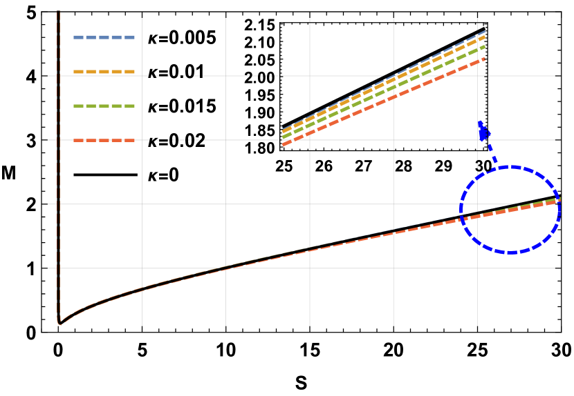
(a) J=0.02,l=5

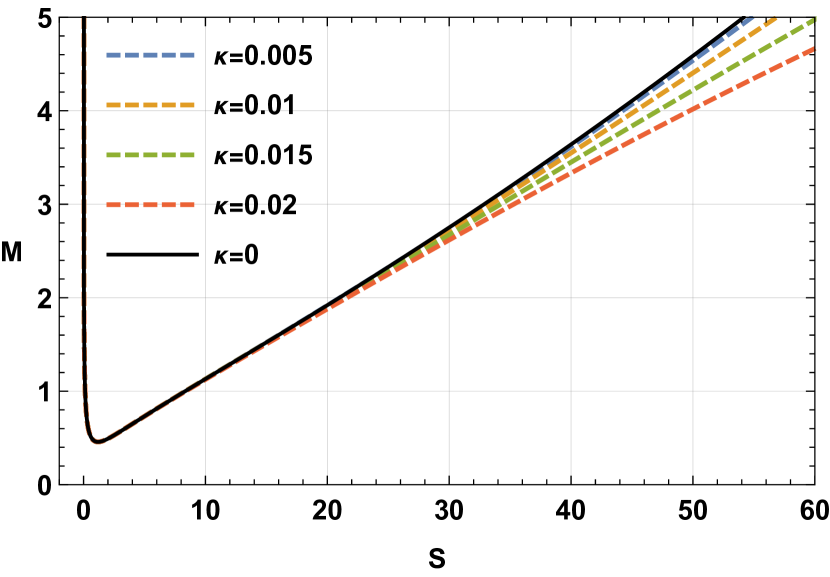
(b) J=0.2,l=3.5

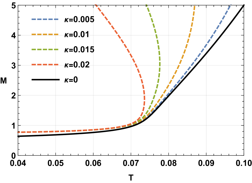
(c) J=0.02,l=5

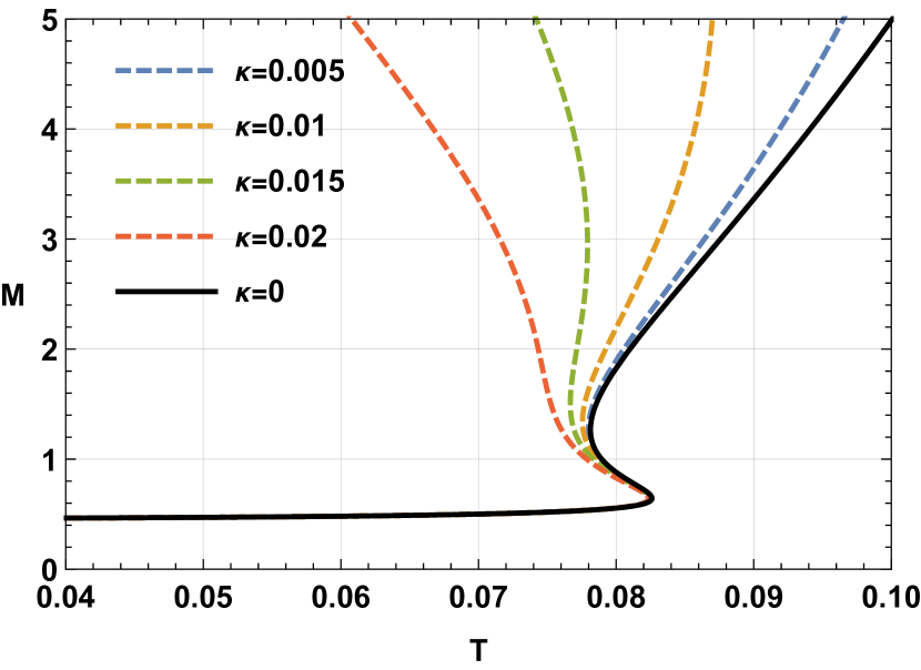
(d) J=0.2,l=3.5

Figure 1: Kerr AdS black hole: Figure (a) and (b) represent $M$ vs $S$ plot for different values of $\kappa,J$ and $l.$ The impact of $\kappa$ parameter is more visible with higher values of $S$. Figure (c) and (d) represents $M$ vs $T$ plot for different value of $\kappa,J$ and $l.$

Similarly, Temperature $T$ is plotted against $S$ in FIG.2. Here we have presented two cases. For the first case, in FIG.2(a), we have considered $J=0.2$ and $l=5$. Here we see four black hole phases. In GB statistics, for critical values of $J$ and $l$, Kerr-Ads black holes exhibit Van der Waals phase transitions as represented by the black solid line in FIG.2(a). In KD statistics, an additional black hole branch which is the ultra-large black hole branch appears as illustrated by the red solid line in FIG.2(c). The appearance of the fourth phase is dependent on the value of the $\kappa$ along with critical values of $J$ and $l.$When the value of $\kappa$ is large, the ultra-large black hole starts to show up at smaller values of KD entropy $S.$ In FIG.2(c), we have considered $J=0.2,l=3.5$ and $\kappa=0.015$ for which we observe four black hole branches. In FIG.2(c) when $S<3.91152$(black dot), a small black hole branch(SBH) is observed represented by a black solid line. Again, within the range $3.91152<S<14.9327$(purple dot), an intermediate black hole branch(IBH) is observed which is represented by the green solid line. A large black hole branch(LBH) is observed within the range $14.9327<S<33.4984$(magenta dot) represented by a blue solid line and finally an ultra large black hole branch(ULBH) is found for the range $S>33.4984.$ On the opposite hand, for $J=0.2$ and $l=3.5$, we observe two black hole branches as shown in FIG.2(b). In FIG.2(d) we consider $J=0.55,l=5$ and $\kappa=0.015$, for which only two black hole branches are observed: a large black hole branch(LBH) for the range $S<53.1069$(blue dot)and a small black hole(SBH) branch for the range $S>53.1069$. The SBH and LBH is represented by the black solid line and the red solid line respectively in FIG.2(d).

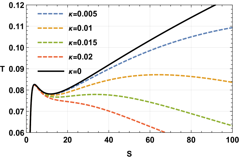
(a) J=0.2, l=3.5

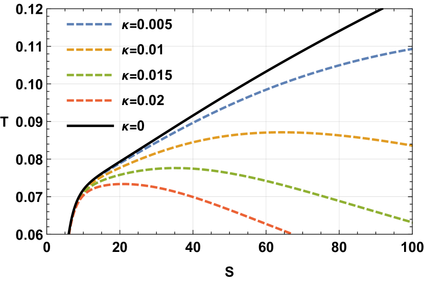
(b) J=0.55, l=5

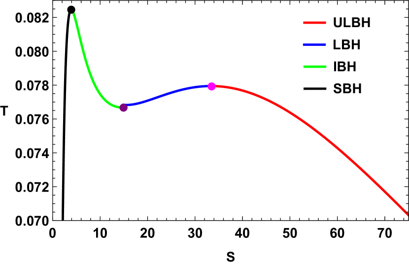
(c) J=0.2, l=3.5, $\kappa$=0.015

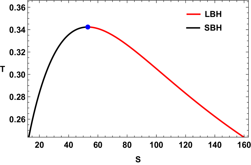
(d) J=0.55, l=1.5, $\kappa$=0.015

Figure 2: Kerr AdS black hole: T vs S plots for different values of $J$ and $l.$ Here SBH, IBH,LBH and ULBH represent small black holes, intermediate black holes, large black holes and ultra large black holes.

To know the thermal stability of these black holes, we calculate the specific heat $(C)$ of the black hole using the formula :

$$C=\frac{dM}{dT}=\frac{dM}{dS}\left(\frac{dT}{dS}\right)^{-1}$$ (18)

The expression for $C$ comes out to be :

$$C=\frac{\mathcal{A}}{\mathcal{B}}$$ (19)

Where,

$$\mathcal{A}=-2\left(\kappa^{2}S^{2}+1\right)\sinh^{-1}(\kappa S)(\pi\kappa l^{2}+\sinh^{-1}(\kappa S))(4\pi^{3}\kappa^{3}J^{2}l^{2}+\pi\kappa l^{2}\sinh^{-1}(\kappa S)^{2}+\\ \sinh^{-1}(\kappa S)^{3})(4\pi^{4}\kappa^{4}J^{2}l^{4}-\pi^{2}\kappa^{2}l^{4}\sinh^{-1}(\kappa S)^{2}-4\pi\kappa l^{2}\sinh^{-1}(\kappa S)^{3}-3\sinh^{-1}(\kappa S)^{4})$$ (20)

and

$$\mathcal{B}=\kappa(48\pi^{8}\kappa^{8}J^{4}l^{8}\sqrt{\kappa^{2}S^{2}+1}+6\pi^{2}\kappa^{2}l^{2}\sinh^{-1}(\kappa S)^{6}(-4\pi\kappa^{2}J^{2}S+l^{2}\sqrt{\kappa^{2}S^{2}+1}-2\pi\kappa^{2}l^{4}S)\\ -2\pi^{3}\kappa^{3}l^{2}\sinh^{-1}(\kappa S)^{5}(\pi\kappa^{2}l^{6}S-24J^{2}(\sqrt{\kappa^{2}S^{2}+1}-\pi\kappa^{2}l^{2}S))\\ -\pi^{4}\kappa^{4}l^{4}\sinh^{-1}(\kappa S)^{4}(l^{4}\sqrt{\kappa^{2}S^{2}+1}-24J^{2}(5\sqrt{\kappa^{2}S^{2}+1}-\pi\kappa^{2}l^{2}S))+96\pi^{5}\kappa^{5}J^{2}l^{6}\sqrt{\kappa^{2}S^{2}+1}\sinh^{-1}(\kappa S)^{3}\\ +8\pi^{6}\kappa^{6}J^{2}l^{6}\sinh^{-1}(\kappa S)^{2}\left(4\pi\kappa^{2}J^{2}S+3l^{2}\sqrt{\kappa^{2}S^{2}+1}\right)+32\pi^{7}\kappa^{7}J^{4}l^{6}(\pi\kappa^{2}l^{2}S+2\sqrt{\kappa^{2}S^{2}+1})\sinh^{-1}(\kappa S)\\ +(3\sqrt{\kappa^{2}S^{2}+1}-20\pi\kappa^{2}l^{2}S)\sinh^{-1}(\kappa S)^{8}+8\pi\kappa l^{2}(\sqrt{\kappa^{2}S^{2}+1}-3\pi\kappa^{2}l^{2}S)\sinh^{-1}(\kappa S)^{7}-6\kappa S\sinh^{-1}(\kappa S)^{9})$$ (21)

In FIG.3, specific heat is plotted against KD entropy S for fix value of $J=0.2$ and $l=3.5.$ Black solid line in FIG.3(a) represents the specific heat at GB statistics($\kappa=0$). As it is illustrated in FIG.3(a), the black line shows only three phases. On the opposite hand, the introduction of KD statistics produces an additional branch for a higher range of entropy. How the phase formation and the singularities are dependent on the $\kappa$ value and entropy range is clearly demonstrated in FIG.3(a). FIG.3(b) is an enlarged version of FIG.3(a) for the entropy range $3.8<S<4.1$. This figure shows how the point at which specific heat diverges, varies with $\kappa$ value. In FIG.3(c) comparison between $C$ VS $S$ plot for $\kappa-0$ and $\kappa=0.015$ is shown for $J=0.2,l=3.5.$ The black solid line is the $C$ vs $S$ plot for $\kappa=0.015$, where specific heat diverges at three points(represented by green dots.) On the other hand, the blue solid line represents $C$ vs $S$ plot in GB statistics ($\kappa=0$). Here only three phases are visible for the same set of values of $J$ and $l.$ Hence the specific heat diverges only at two points. In FIG.3(d), the $C$ vs $S$ graph is shown for $J=0.55,l=1.5$. For this set of values, in the $\kappa=0$ case, the specific heat does not diverge at any point hence there is no phase transition but for non-zero values of $\kappa$, we observe at least one point at which the specific heat diverges.

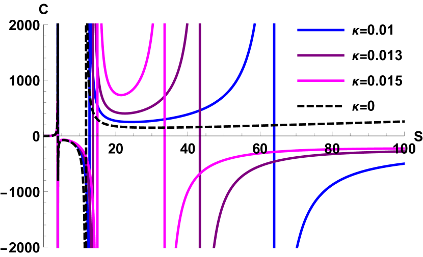
(a) C vs S plot($J=0.2$ and $l=3.5$) for the range $0<S<100$

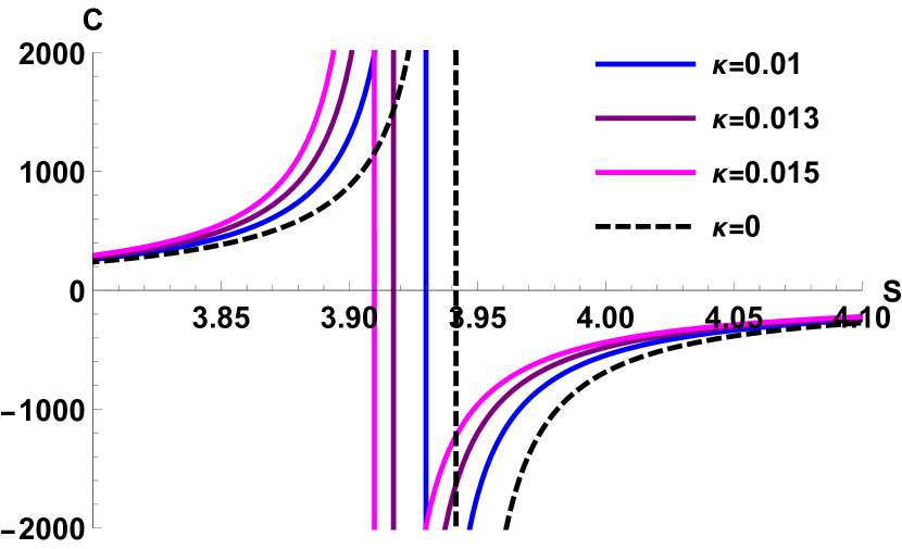
(b) Closer look at $3.8<S<4.1$ range($J=0.2$ and $l=3.5$)

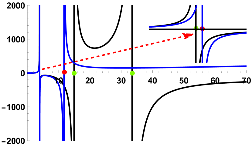
(c) For the blue solid line, $\kappa=0$ and for black solid line $\kappa=0.015$

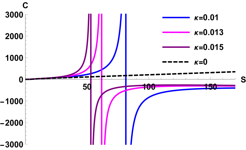
(d) Here $J=0.55,l=1.5$

Figure 3: Kerr AdS black hole: C vs S plots.

It is well known that each point at which specific heat diverges represents a phase transition point. This is explained in FIG.4(a), where we see four black hole phases: a small black hole branch(SBH), an intermediate black hole branch(IBH), a large black hole branch(LBH), and an ultra-large black hole branch(ULBH).

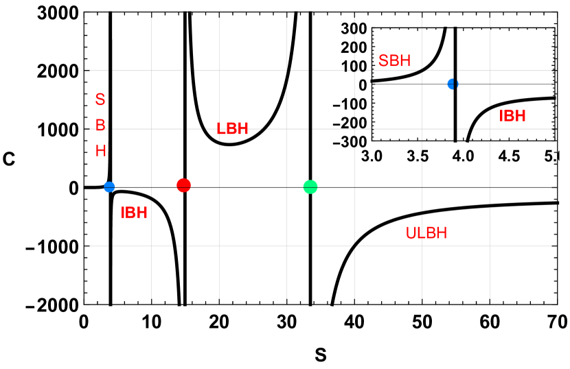
(a) C vs S plot at $J=0.2,\kappa=0.015$ and $l=3.5$

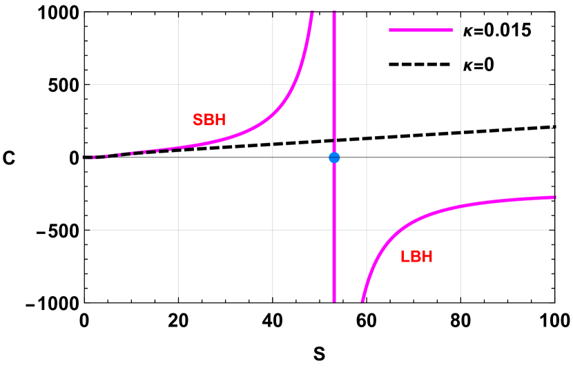
(b) C vs S at $J=0.55,\kappa=0.015$ and $l=1.5$

Figure 4: Kerr AdS black hole: C vs S plots.

There are three phase transition points at which the specific heat diverges represented by blue dot($S=3.91152$) red dot($S=14.9327$) and green dot($S=33.4984$). Within the range $S<3.91152$, a small black hole is observed with positive specific heat, hence it is a thermally stable branch. Within the range $3.91152<S<14.9327$, an intermediate black hole branch is observed with negative specific heat, hence the branch is thermally not stable. Again within the range $14.9327<S<33.4984$, a thermally stable large black hole branch is observed as the specific heat in that range is found to be positive. Finally, a thermally unstable ultra-large black hole is found within the $S>33.4984$ range where the specific heat is negative. In FIG.4(b), $C$ is plotted agaist $S$ for $J=0.55$ and $l=1.5$. Here we observe a Davies-type phase transition point at $S=53.1069$(represented by the blue dot) where the specific heat diverges. For the range $S<53.1069$, a stable small black hole branch(SBH) is seen and for $S>53.1069$, an unstable large black hole branch(LBH) is seen. On the contrary, in GB statistics we do not get any Davies-type phase transition as shown by the black dashed line in FIG.4(b).

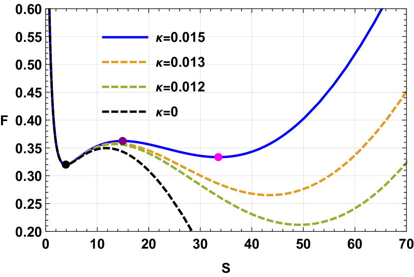
(a) F vs S plot at $J=0.2$ and $l=3.5$

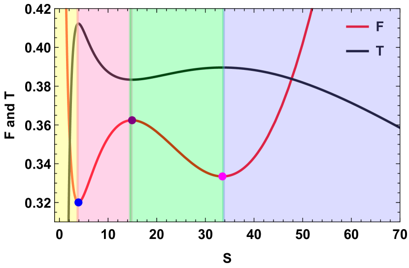
(b) BH Phases in F/T vs S plot($J=0.2,l=3.5$)

(c) F vs S plot at $J=0.55$ and $l=5$

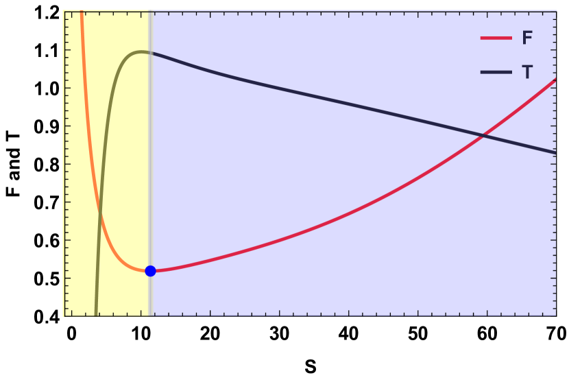
(d) BH Phases in F/T vs S plot($J=0.55,l=5$)

Figure 5: Kerr AdS black hole: F vs S plots.

Gibbs Free energy($F$) provides valuable insight into the characteristics of phase transitions in black holes. The free energy is calculated using the following relation:

$$F=M-TS$$ (22)

here T is the horizon temperature calculated in the equation 17. Using equation 17 and 16, F is calculated as :

$$F=\frac{\mathcal{C}}{\mathcal{D}}$$ (23)

Where,

$$\mathcal{C}=\frac{\kappa S\left(4\pi^{4}\kappa^{4}J^{2}l^{4}-\pi^{2}\kappa^{2}l^{4}\sinh^{-1}(\kappa S)^{2}-4\pi\kappa l^{2}\sinh^{-1}(\kappa S)^{3}-3\sinh^{-1}(\kappa S)^{4}\right)}{\sqrt{\kappa^{2}S^{2}+1}}\\ +2\sinh^{-1}(\kappa S)\left(\pi\kappa l^{2}+\sinh^{-1}(\kappa S)\right)\left(4\pi^{3}\kappa^{3}J^{2}l^{2}+\pi\kappa l^{2}\sinh^{-1}(\kappa S)^{2}+\sinh^{-1}(\kappa S)^{3}\right)$$ (24)

And

$$\mathcal{D}=4\pi^{3/2}\kappa^{5}l^{2}\left(\frac{\sinh^{-1}(\kappa S)}{\kappa}\right)^{3/2}\sqrt{\pi l^{2}+\frac{\sinh^{-1}(\kappa S)}{\kappa}}\sqrt{\frac{4\pi^{3}\kappa^{3}J^{2}l^{2}+\pi\kappa l^{2}\sinh^{-1}(\kappa S)^{2}+\sinh^{-1}(\kappa S)^{3}}{\kappa^{3}}}$$ (25)

FIG.5 represents two scenarios where from the free energy plot, the number of black hole branches can be identified. In FIG5(a) and FIG.5(b), it is seen that for non-zero $\kappa$ value there are at least two black hole branches. On the other hand, the black dashed line in FIG5(a) and FIG.5(b) shows that there are either three or one black hole branches in GB statistics. In FIG.5(c), when $J=0.2,l=3.5,\kappa=0.015$ are taken, the four phases are visible(for better comparability $T$ vs $S$ plot is used as reference). In FIG.5(c), black holes in the yellow region are the small black holes, black holes within the pink region are intermediate black holes, black holes within the green region are large black holes, and finally black holes in the blue region are an ultra large black hole. The phase transitioning points are shown in multicolored dots in the $F$ vs $S$ plot represented by the red solid line in FIG.5(b). Similarly in FIG.5(d) we have used $J=0.2,l=3.5,\kappa=0.015$, where the black holes in the yellow region are small black holes and the black holes lie in the blue region are the large black holes. The phase transition phenomenon is also clearly visible in FIG.6, where parametric plot between $F$ vs $T$ is shown for $J=0.2,l=3.5$ and $\kappa=0.015$

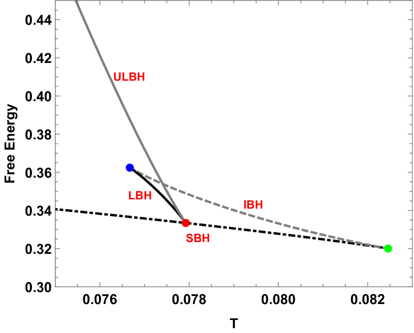
(a) F vs T plot at $J=0.2$ and $l=3.5$

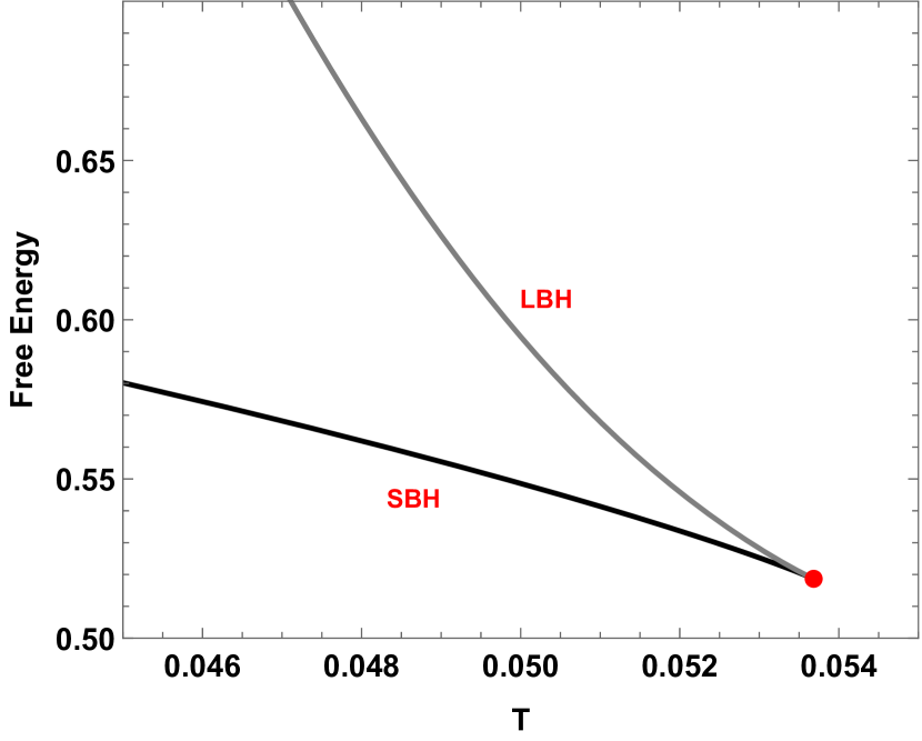
(b) F vs T plot at $J=0.55$ and $l=5$

Figure 6: Kerr AdS black hole: F vs T plots.

Next, we do the free energy landscape analysis to estimate the stability of black holes from the free energy plot. To construct the free energy landscape, we write the off-shell free energy as[173] :

$$F_{e}=F-T_{e}S=-\frac{2\pi^{3/2}l^{2}ST_{e}\sqrt{\frac{\sinh^{-1}(\kappa S)}{\kappa}}-\sqrt{\frac{\pi\kappa l^{2}+\sinh^{-1}(\kappa S)}{\kappa}}\sqrt{\frac{4\pi^{3}\kappa^{3}J^{2}l^{2}+\pi\kappa l^{2}\sinh^{-1}(\kappa S)^{2}+\sinh^{-1}(\kappa S)^{3}}{\kappa^{3}}}}{2\pi^{3/2}l^{2}\sqrt{\frac{\sinh^{-1}(\kappa S)}{\kappa}}}$$ (26)

Here $T_{e}$ is the ensemble temperature. Taking the first derivative of the off-shell or generalized free energy

$$\frac{\partial F_{e}}{\partial S}=(T-T_{e})$$

Hence, a physical black hole is only possible at the extremal point of the off-shell free energy, where $\frac{\partial F_{e}}{\partial S}$ is zero. Again, it can be proved that the second order derivative of $F_{e}$ is related to sign of specific heat through the relation :

$$\left(\frac{\partial^{2}F_{e}}{\partial^{2}S}\right)_{T_{e}=T}=\frac{\partial T}{\partial M}\frac{\partial M}{\partial S}=\frac{T}{C}$$

Hence at the maximum value of off-shell free energy, the black hole is thermally unstable and vice versa. The free energy landscape for Kerr ads black hole in GB statistics is analyzed in [174]. We plot the free energy landscape for Kerr ads in KD statistics in the FIG.7. For this particular analysis, we have considered five temperatures $T_{1}=0.076,T_{2}=0.077,T_{3}=0077924,T_{4}=0.07742,T_{5}=0.080$ and kept $J=0.2,l=3.5$ and $\kappa=0.015$ fixed. Although all the figures are almost self-deprecating, we will explain one of the scenarios in detail. For instance, if we consider the FIG.7(c) where we have plot $F_{e}$ for $T_{e}=T_{2}=0.077$, then we see four black holes in the $F_{e}$ vs $S$ plot which are located at the extremum points. As it is illustrated in FIG.7(a), the $T=T_{2}$ line cuts the $F$ vs $T$ graph at four points: B at SBH, K at IBH, K’ at LBH, and I at ULBH. These four points represent four physical black holes in FIG.7(a). The B point is located at the global minima of the graph, hence this black hole is thermally and globally stable. The K point lies in the local maxima point, this point is thermally and locally unstable. The K’ point is situated in the local minima point, hence this point is thermally stable but globally unstable, and finally, the I point is at global maxima hence this point is both globally and thermally unstable. Therefore we can infer from FIG.7 that points $A,B,C,D,E$ are both thermally and globally stable, $K^{\prime},H,D_{3}$ are thermally stable but only locally stable, $K,G,H^{\prime}$ are thermally and locally unstable and finally $F,J,I,D_{2},L$ are both globally and thermally unstable.

(a)

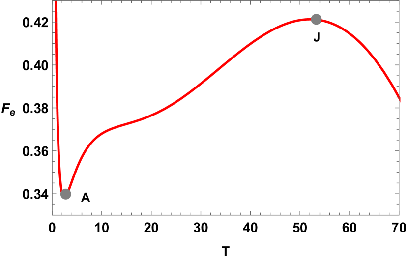
(b) $T_{e}=0.076$

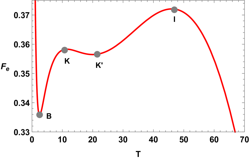
(c) $T_{e}=0.077$

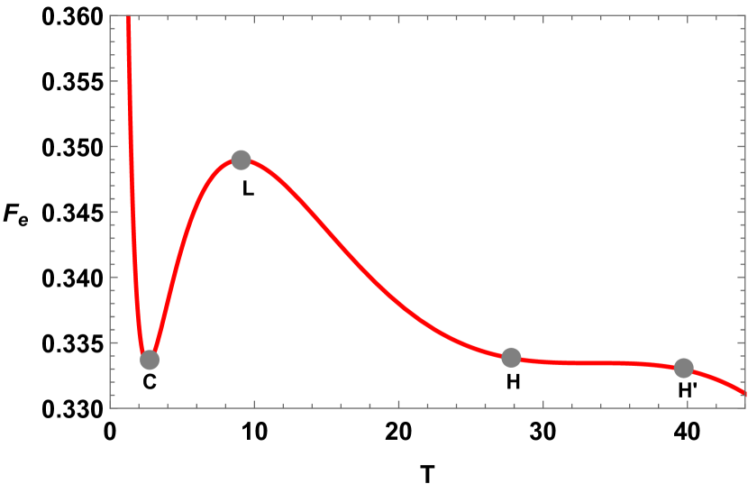
(d) $T_{e}=0.077924$

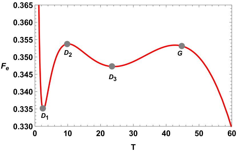
(e) $T_{e}=0.07742$

(f) $T_{e}=0.080$

Figure 7: Kerr AdS black hole: Free energy landscape. For these plots, we have kept $J=0.2,l=3.5$ and $\kappa=0.015$ fixed.

III Thermodynamic topology of Kerr-Ads black holes

Using eq.2 and eq.16, we write the off shell free energy as :

$$\mathcal{F}=M-\frac{S}{\tau}\\ =-\frac{2\pi^{3/2}l^{2}S\sqrt{\frac{\sinh^{-1}(\kappa S)}{\kappa}}-\tau\sqrt{\frac{\pi\kappa l^{2}+\sinh^{-1}(\kappa S)}{\kappa}}\sqrt{\frac{4\pi^{3}\kappa^{3}J^{2}l^{2}+\pi\kappa l^{2}\sinh^{-1}(\kappa S)^{2}+\sinh^{-1}(\kappa S)^{3}}{\kappa^{3}}}}{2\pi^{3/2}l^{2}\tau\sqrt{\frac{\sinh^{-1}(\kappa S)}{\kappa}}}$$ (27)

Using eq.3, components of the vector $\phi$ are found to be :

$$\phi^{r} = \frac{\alpha_{1}}{\beta_{1}}$$ (28)

$$\phi^{\Theta} = -\cot\Theta~{}\csc\Theta.$$ (29)

where

$$\alpha_{1}=-4\pi^{4}\kappa^{4}J^{2}l^{4}\tau-4\pi^{3/2}\kappa^{4}l^{2}\sqrt{\kappa^{2}S^{2}+1}\left(\frac{\sinh^{-1}(\kappa S)}{\kappa}\right)^{3/2}\sqrt{\pi l^{2}+\frac{\sinh^{-1}(\kappa S)}{\kappa}}\\ \sqrt{\frac{4\pi^{3}\kappa^{3}J^{2}l^{2}+\pi\kappa l^{2}\sinh^{-1}(\kappa S)^{2}+\sinh^{-1}(\kappa S)^{3}}{\kappa^{3}}}+\pi^{2}\kappa^{2}l^{4}\tau\sinh^{-1}(\kappa S)^{2}+4\pi\kappa l^{2}\tau\sinh^{-1}(\kappa S)^{3}+3\tau\sinh^{-1}(\kappa S)^{4}$$ (30)

and

$$\beta_{1}=4\pi^{3/2}\kappa^{4}l^{2}\tau\sqrt{\kappa^{2}S^{2}+1}\left(\frac{\sinh^{-1}(\kappa S)}{\kappa}\right)^{3/2}\sqrt{\pi l^{2}+\frac{\sinh^{-1}(\kappa S)}{\kappa}}\sqrt{\frac{4\pi^{3}\kappa^{3}J^{2}l^{2}+\pi\kappa l^{2}\sinh^{-1}(\kappa S)^{2}+\sinh^{-1}(\kappa S)^{3}}{\kappa^{3}}}$$ (31)

Next, we find the zero points or the defects of the vector field. One zero point of the vector field is always $\Theta=\frac{\pi}{2}$ due to the smart choice of the $\Theta$- component of the field. To find the other zero points, we calculate an expression for $\tau$ by solving $\phi^{S}=0$, which is obtained as:

$$\tau=\frac{4\pi^{3/2}\kappa^{4}l^{2}\sqrt{\kappa^{2}S^{2}+1}\left(\frac{\sinh^{-1}(\kappa S)}{\kappa}\right)^{3/2}\sqrt{\frac{\pi\kappa l^{2}+\sinh^{-1}(\kappa S)}{\kappa}}\sqrt{\frac{4\pi^{3}\kappa^{3}J^{2}l^{2}+\pi\kappa l^{2}\sinh^{-1}(\kappa S)^{2}+\sinh^{-1}(\kappa S)^{3}}{\kappa^{3}}}}{-4\pi^{4}\kappa^{4}J^{2}l^{4}+\pi^{2}\kappa^{2}l^{4}\sinh^{-1}(\kappa S)^{2}+4\pi\kappa l^{2}\sinh^{-1}(\kappa S)^{3}+3\sinh^{-1}(\kappa S)^{4}}$$ (32)

One of the key aspects of the study of black hole thermodynamics from a topological perspective is the calculation of topological charge. To calculate the topological charge, we need to identify the branches of the black hole in the $\tau$ vs $S$ graph.From the thermodynamic study, we understand that there are two possible scenarios. In the first scenario, four distinct black hole phases can occur: small black hole (SBH), intermediate black hole (IBH), large black hole (LBH), and ultra-large black hole (ULBH). In the second scenario, only two black hole phases are observed: a small black hole (SBH) and a large black hole (LBH). We present the two scenarios and the corresponding topological charge in the following paragraph.
In the first case, we present the plot of the KD entropy $S$ as a function of $\tau$ in Fig. 8, using the parameters $J=0.2$, $l=3.5$, and $\kappa=0.0015$. This plot reveals four distinct branches of black holes.

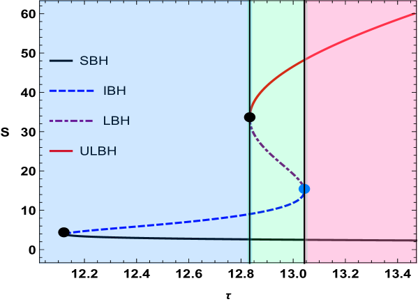
Figure 8: Kerr-Ads black hole : $\tau$ vs $S$ plot. Here we have taken $J=Q=0.2$ and $l=3.5$

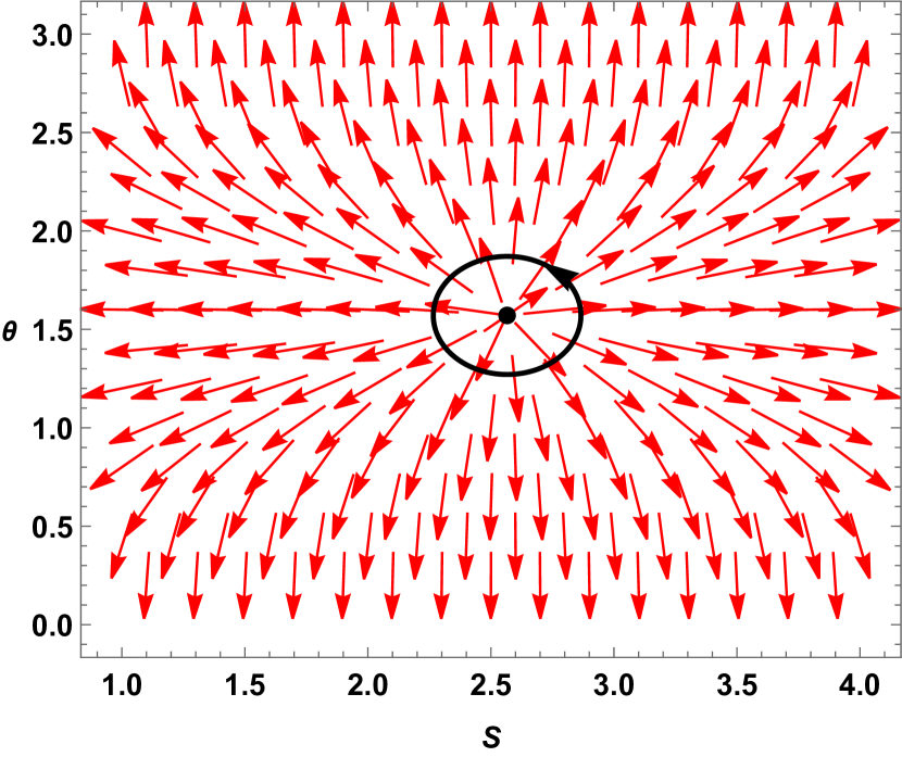
(a)

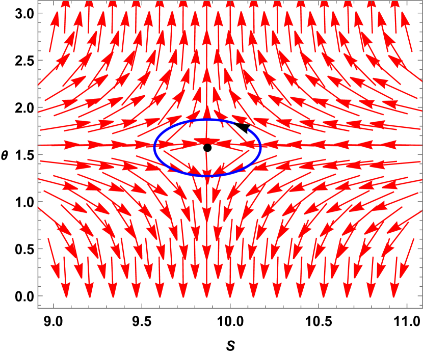
(b)

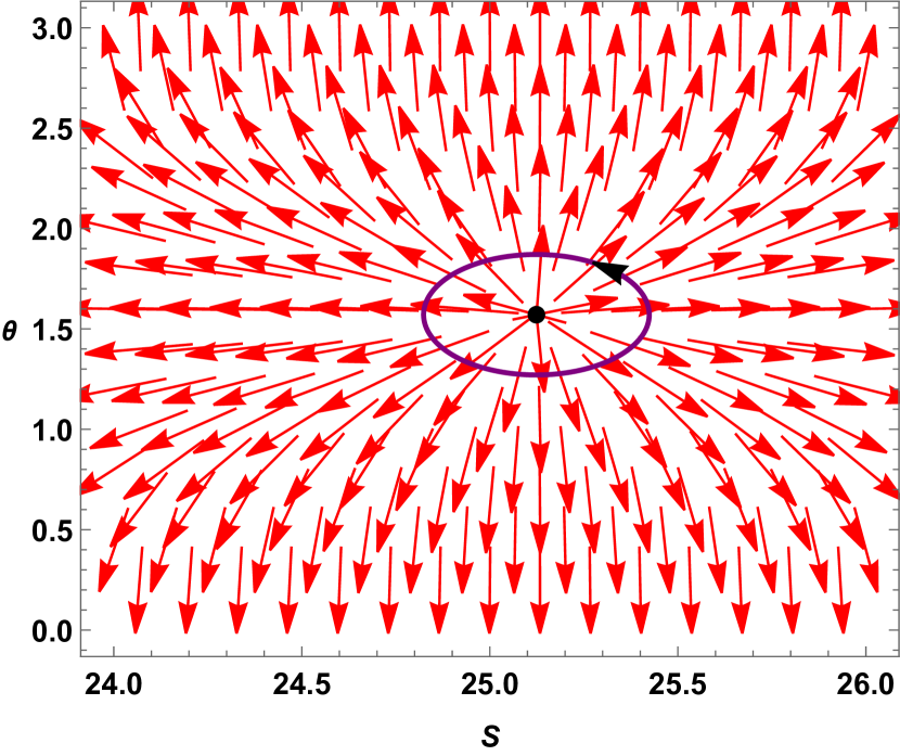
(c)

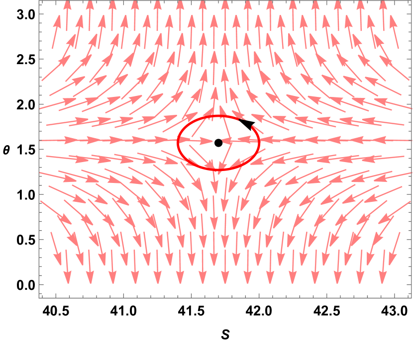
(d)

Figure 9: Kerr-Ads black holes: Vector plots of normalized ($\phi^{S}$,$\phi^{\Theta}$) field on the $S-\Theta$ plane

For the calculation of topological charge, one needs to find the winding number around each zero point of the normalized vector field $(n^{1},n^{2})$ for a particular value of $\tau$. For example for $\tau=12.9$, we get four zero point at $S=2.5657$, $S=9.8711$, $S=25.1238$, and $S=41.7004$. In Figs. 9(a), 9(b), 9(c), and 9(d), we provide vector plots illustrating the normalized components $\phi^{S}$ and $\phi^{\Theta}$ for $\tau=12.9$. Next, contours are formed around each zero point using the eq.9 as :

$$\begin{cases}S=0.3cos\nu+r_{0},\\ \\ \theta=0.2sin\nu+\frac{\pi}{2},\end{cases}$$ (33)

where we have set $r_{1}=0.3$ and $r_{2}=0.2.$ and $r_{0}$ is the zero point around which contours are formed. Substituting the value of $S$ and $\Theta$ in the expression of the normalized field $(n^{1},n^{2})$ we find the deflection using eq.11. This is called the parameterization of the contours. After solving the contour integration, we substitute the value of deflection in the eq.10 and find the winding number. The winding number around a zero point represents the winding number for the entire branch in which the zero point lies. For example, the zero point $S=2.5657$ is on the SBH, hence the winding number around this zero point represents the winding number for the whole branch.
Fig. 10 displays four contour plots, each illustrating the computation of the winding number around the identified zero points. The solid black and red colored contour represents the winding number for SBH and ULBH respectively. On the other hand, the dashed blue colored contour and the dot-dashed purple colored contour represent the winding number for IBH and LBH respectively. As depicted by the black contour in Fig. 10(a), the winding number for $S=2.5657$ (SBH branch) is $+1$. In contrast, Fig. 10(b) shows that the winding number for $S=9.8711$ (IBH branch) is $-1$. Similarly, the dot-dashed purple contour in Fig. 10(c) indicates that the winding number for $S=25.1238$ (LBH branch) is $+1$. Finally, the red contour in Fig. 10(d) demonstrates that the winding number for $S=41.7004$ (ULBH branch) is $-1$. A positive winding number implies stability for the small and large black hole branches. Conversely, the intermediate and ultra-large black hole branches, having negative winding numbers, are unstable. To find the topological charge, all the individual winding number of each branch is added. Hence the total topological charge of the Kerr-AdS black hole in KD statistics is calculated as $\Sigma_{i}w_{i}=1-1+1-1=0$. A creation or generation point is the exact location where an unstable black hole branch vanishes and a stable black hole branch begins. Conversely, an annihilation point is where a stable black hole branch vanishes and an unstable black hole branch starts. Here two annihilation point is identified at $(\tau_{c},S)=(12.1276,3.9115),(12.833,33.4983)$, marked by black dots in Fig. 8 and a generation point is observed at $(\tau_{c},S)=(13.0428,14.9326)$ marked by the blue dot.

(a)

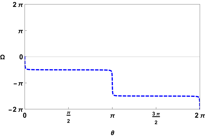
(b)

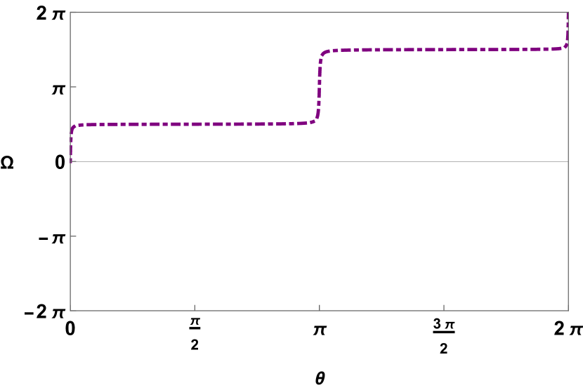
(c)

(d)

Figure 10: Kerr-Ads black holes: Winding number calculations for Kerr-Ads black holes. The black solid line in Fig.10(a) and purple dot dashed line in Fig.10(c) represent the winding number for SBH and LBH respectively which equals $+1$ and the blue solid line in Fig.10(b). The red solid line in Fig.10(d) represents the winding number for IBH and ULBH respectively which equals $-1.$

Moving on to the second case, where two black hole branches are observed as shown in Fig.11(a): a small black hole branch(SBH) and a large black hole branch (LBH). The winding number for SBH is $+1$ which means it is stable and that for LBH is found to be $-1$ which suggests it is an unstable branch. Moreover, we found an annihilation point in $(\tau=2.9211,S=53.1069)$ represented by the black dot in the Fig.11(a).

(a)

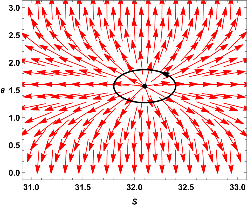
(b)

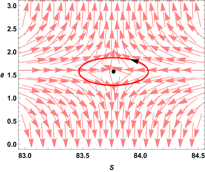
(c)

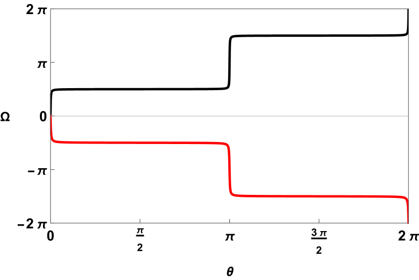
(d)

Figure 11: Kerr-Ads black holes: In Fig.11(a), $\tau$ vs $S$ is plotted for Kerr-Ads black holes when $J=Q=0.5,l=1$ and $\kappa=0.015$ is taken. In Fig.11(b) and Fig.11(c) vector plots are shown in $S-\Theta$ plane where the zero point (S,$\Theta$)= $(35.5982,\pi/2)$ in Fig.11(b) is on the SBH and the zero point (S,$\Theta$)= $(82.9878,\pi/2)$ in Fig.11(c) is on the LBH. The winding number calculation is shown in Fig.26(d) where the black solid line in Fig.11(d) represents winding number for SBH which equals to $+1$ and the red solid line in Fig.11(d) represents winding number for LBH which equals to $-1.$

In Fig. 12(a) and Fig. 12(b), we show the variation of $\kappa$ with $J=0.2$, $l=3.5$, and with $J=0.5$, $l=1$, respectively. Fig. 12(c) illustrates the variation of $J$ with $l=3.5$, and $\kappa=0.015$ held constant. Fig. 12(d), depict the variation of $l$ with $J=0.2$ and $\kappa=0.015$ fixed.
The number of branches in the $\tau$ vs $S$ graph changes with variations in the values of $J$ and $l$. We observe either four or two branches depending on the specific values of these thermodynamic parameters. However, the topological charge remains invariant when the values of $J$, $l$, and $\kappa$ are varied. Most importantly, a change in the topological charge of the Kerr-Sen AdS black hole is observed when transitioning from the GB statistics framework to the KD statistics framework. In GB statistics, the topological charge of the black hole is $+1$, whereas in the KD statistics formalism, it is found to be $0$.

(a)

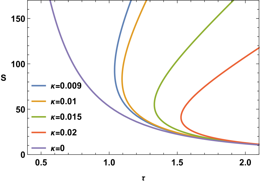
(b)

(c)

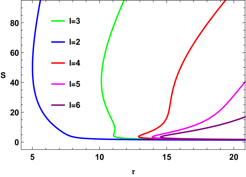
(d)

Figure 12: Variation of $\tau$ vs $S$ plots for Kerr-Ads black holes with different thermodynamic parameter.

In conclusion, for the Kerr-Sen-ads black hole in KD statistics, the topological charge is $0$ and it is observed that, the topological charge is independent of other thermodynamic parameters.

IV Thermodynamic geometry of the Kerr-AdS black holes

The line element for the Ruppeiner metric in the Kerr-AdS black hole could be written as :

$$dS_{R}^{2}=\frac{1}{T}\left(\frac{\partial^{2}M}{\partial S^{2}}dS^{2}+\frac{\partial^{2}M}{\partial J^{2}}dJ^{2}+2\frac{\partial^{2}M}{\partial S\partial J}dSdJ\right)$$

and the line element for the GTD metric in the Kerr-AdS black hole is given by:

$$dS_{G}^{2}=S\left(\frac{\partial M}{\partial S}\right)\left(-\frac{\partial^{2}M}{\partial S^{2}}dS^{2}+\frac{\partial^{2}M}{\partial J^{2}}dJ^{2}\right)$$

We see here from Fig.13 that the Ruppeiner scalar is plotted against the Kaniadakis entropy for $J=0.2$ and $L=3.5$. There are curvature singularities in the Ruppeiner scalar curves for every value of the Kaniadakis parameter and for $\kappa=0.015$ the Ruppeiner curve is separately shown in Fig.13(b) which shows the presence of a singularity at $S=1.184$. From Fig.13(d) we see that there are two more curvature singularities at $S=16.492$ and $33.147$ for the same J and L values for $\kappa=0.015$. Similarly from Fig.14(b) for $J=0.55$ and $L=1.5$ we see only one singularity at $S=53.013$. These singularities found in the Ruppeiner scalar curves do not match with the points of Davies type phase transitions found in the specific heat capacity curves for $\kappa=0.015$ for the same J and L values. The GTD curves shown in Fig.15(b) and Fig.15(d) show a curvature singularity at $S=3.911$ and two more singularities at $S=14.933$ and $33.498$ respectively for $J=0.2$ and $L=3.5$. For $J=0.55$ and $L=1.5$ we see from Fig.16(b) that there happens to be only one singularity at $S=53.107$. Unlike Ruppeiner scalar curves the singularities in the GTD scalar curves match exactly with the points of Davies type phase transitions obtained in the heat capacity curves.

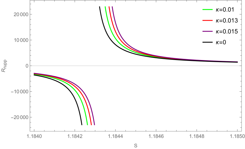
(a) $3.8<S<4.1$ for all $\kappa$

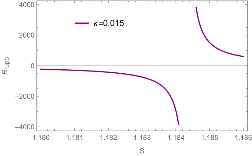
(b) For $\kappa=0.015$

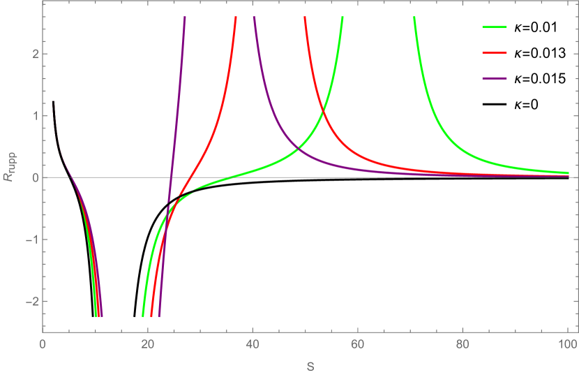
(c) $S>4.1$ for all $\kappa$

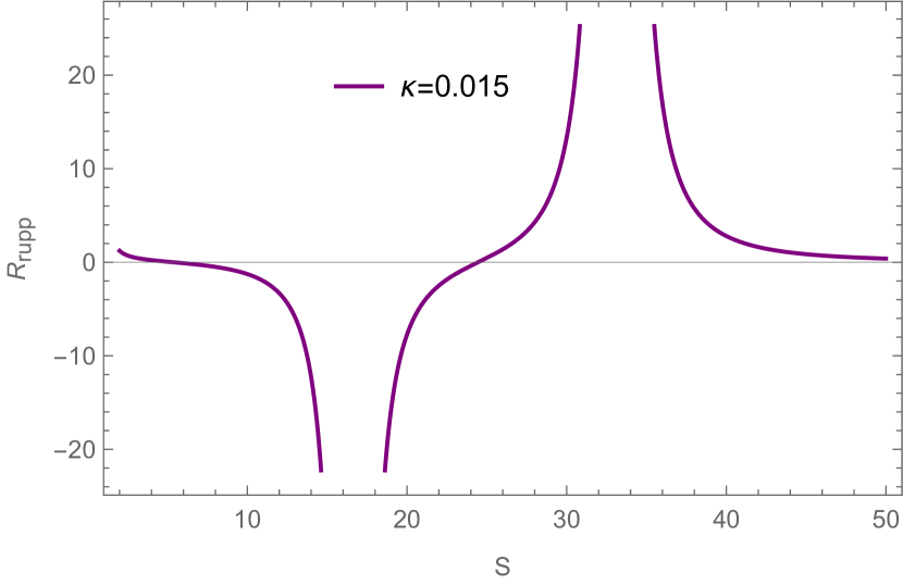
(d) For $\kappa=0.015$

Figure 13: The Ruppeiner scalar versus Entropy plot for Kerr-AdS black hole for $J=0.2$ and $L=3.5$.

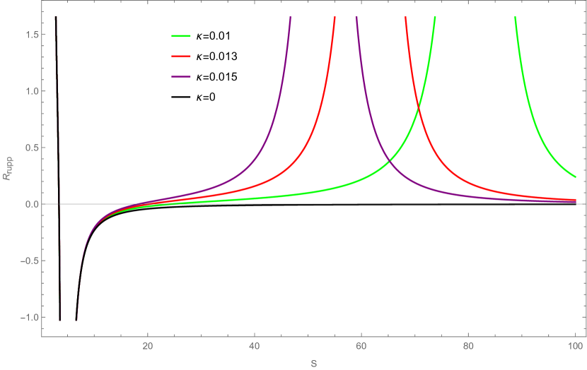
(a) For all $\kappa$

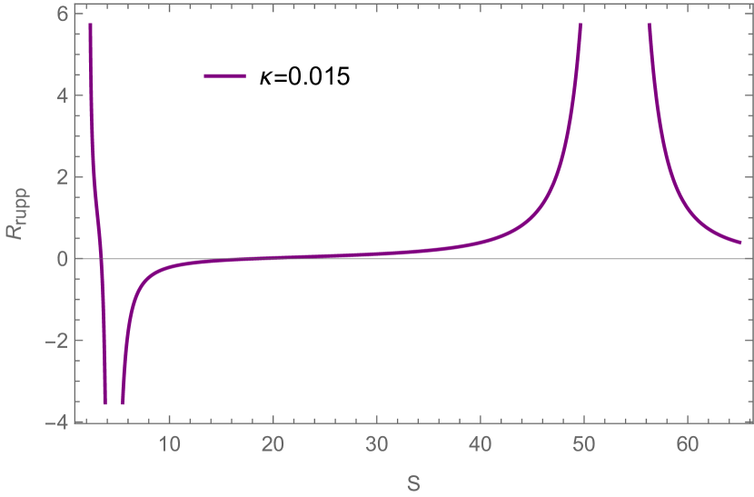
(b) For $\kappa=0.015$

Figure 14: The Ruppeiner scalar versus Entropy plot for Kerr-AdS black hole for $J=0.55$ and $L=1.5$.

(a) $3.8<S<4.1$ for all $\kappa$

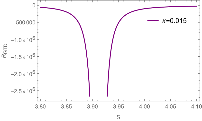
(b) For $\kappa=0.015$

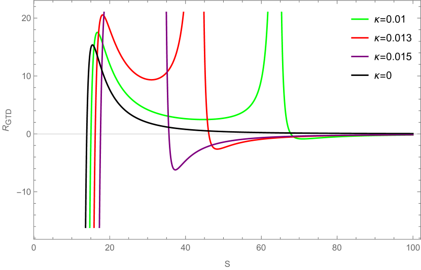
(c) $S>4.1$ for all $\kappa$

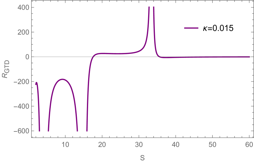
(d) For $\kappa=0.015$

Figure 15: The GTD scalar versus Entropy plot for Kerr-AdS black hole for $J=0.2$ and $L=3.5$.

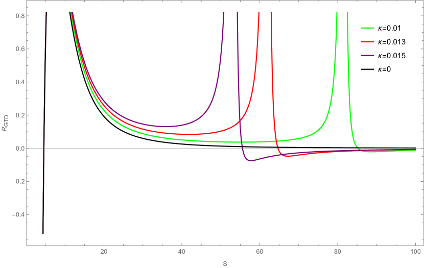
(a) For all $\kappa$

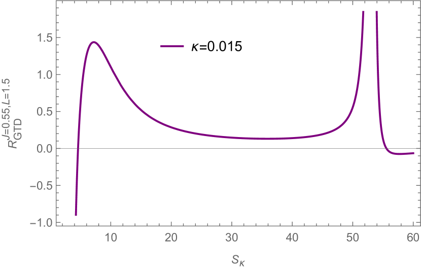
(b) For $\kappa=0.015$

Figure 16: The GTD scalar versus Entropy plot for Kerr-AdS black hole for $J=0.55$ and $L=1.5$.

V Thermodynamics of Kerr-Sen-Ads Black holes

The ADM mass of the Kerr-sen-Ads black hole in terms of entropy is obtained to be

$$M=\frac{\sqrt{S_{\text{BH}}+\pi l^{2}}\sqrt{\pi l^{2}S_{\text{BH}}\left(S_{\text{BH}}+2\pi Q^{2}\right)+S_{\text{BH}}^{3}+4\pi^{3}J^{2}l^{2}}}{2\pi^{3/2}l^{2}\sqrt{S_{\text{BH}}}}$$ (34)

The mass is converted to the KD mass as :

$$M_{KD}=\frac{\sqrt{\pi\kappa l^{2}+\sinh^{-1}(\kappa S)}\sqrt{4\pi^{3}\kappa^{3}J^{2}l^{2}+\pi\kappa l^{2}\sinh^{-1}(\kappa S)\left(2\pi\kappa Q^{2}+\sinh^{-1}(\kappa S)\right)+\sinh^{-1}(\kappa S)^{3}}}{2\pi^{3/2}\kappa^{3/2}l^{2}\sqrt{\sinh^{-1}(\kappa S)}}$$ (35)

The temperature can be evaluated from eq.35 as :

$$T=\frac{dM_{KD}}{dS}\\ =\frac{-4\pi^{4}\kappa^{4}J^{2}l^{4}+\pi^{2}\kappa^{2}l^{2}\left(l^{2}+2Q^{2}\right)\sinh^{-1}(\kappa S)^{2}+4\pi\kappa l^{2}\sinh^{-1}(\kappa S)^{3}+3\sinh^{-1}(\kappa S)^{4}}{4\pi^{3/2}\kappa^{4}l^{2}\sqrt{\kappa^{2}S^{2}+1}\left(\frac{\sinh^{-1}(\kappa S)}{\kappa}\right)^{3/2}\sqrt{\pi l^{2}+\frac{\sinh^{-1}(\kappa S)}{\kappa}}\sqrt{\frac{4\pi^{3}\kappa^{3}J^{2}l^{2}+2\pi^{2}\kappa^{2}l^{2}Q^{2}\sinh^{-1}(\kappa S)+\pi\kappa l^{2}\sinh^{-1}(\kappa S)^{2}+\sinh^{-1}(\kappa S)^{3}}{\kappa^{3}}}}$$ (36)

Similar to the Kerr-Ads black holes, the influence of the KD parameter $\kappa$ on black hole mass becomes more significant at higher values of KD entropy $S$. As illustrated in FIG.17(a) and FIG.17(b), a smaller $\kappa$ corresponds to a wider range of KD entropy $S$ where $M_{KD}$ closely resembles $M_{BH}$. For Kerr-Sen-Ads black holes, apart from the angular momentum $J$ and Ads length $l$, the charge $Q$ proves to be a crucial parameter in determining the thermodynamic property of the black hole. In FIG.17(a) and FIG.17(b), the KD mass of the black hole in KD statistics is plotted for different values of $\kappa$ while keeping $J=0.2,Q=0.2,l=3.5$ and $J=0.5,Q=0.5,l=1$ fixed respectively. The behavior of mass with increasing $\kappa$ values is similar to that observed in Kerr-AdS black holes. In FIG.17(c) and FIG.17(d), mass is plotted against temperature for a better representation of the dependence of mass on the value of $\kappa$. The inclusion of the charge $Q$ parameter is important in determining the number of branches in $M$ vs $T$ graph. Depending on the values of $Q$ along with $J$ and $l$ we see either four branches or two branches in the $M$ vs $T$ graph for non-zero values of $\kappa$. For example in FIG.17(c), if we consider $J=0.2,Q=0.2,l=3.5$, then four branches are observed and on the other hand if $J=0.5,Q=0.5,l=1$ is taken then there are two branches as shown in FIG.1(d).

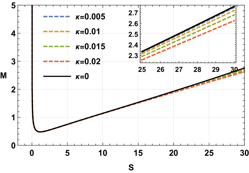
(a) J=0.2, Q=0.2, l=3.5

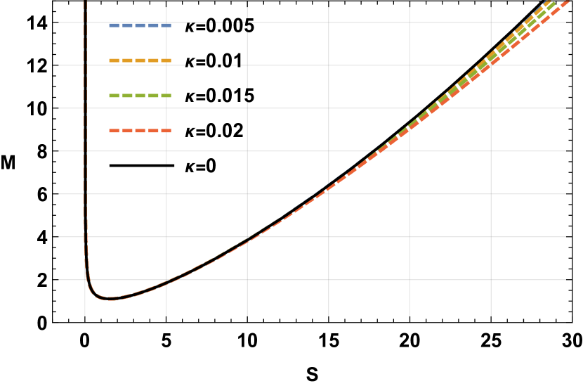
(b) J=0.5, Q=0.5, l=1

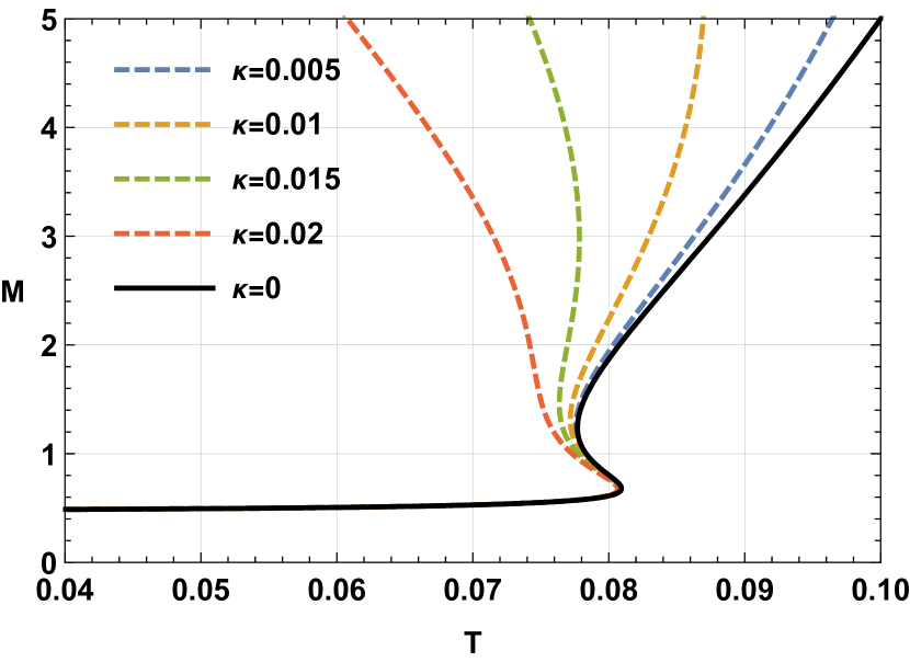
(c) J=0.2, Q=0.2, l=3.5

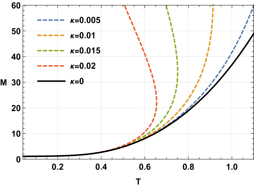
(d) J=0.5, Q=0.5 ,l=1

Figure 17: Kerr-sen-AdS black hole: Figure (a) and (b) represents $M$ vs $S$ plot for different value of $\kappa,J,Q$ and $l.$ The impact of $\kappa$ parameter is more visible with higher values of $S$. Figure (c) and (d) represents $M$ vs $T$ plot for different value of $\kappa,J,Q$ and $l.$

Temperature $T$ is plotted against $S$ in FIG.18 where two possible phase transition types in Kerr-Sen-Ads black hole are presented. In the first case, we have taken $J=0.2,Q=0.2$ and $l=3.5$ in FIG.18(a) for which four black hole phases appeared. The black solid line in FIG.18(a) represents the Van der Waals-like phase transition in GB statistics. For the Kerr-Sen-Ads black hole also, an additional black hole branch comes into sight in KD statistics. We call this branch as the ultra-large black hole branch illustrated by the red solid line in FIG.18(c). In FIG.18(c) four black hole branches are detected: one small black hole branch(SBH) for the range $S<4.1113$(up to the black dot) represented by a black solid line, an intermediate black hole branch(IBH) within the range $4.1113<S<14.1983$(upto the purple dot) represented by a green solid line, a large black hole branch(LBH) within the range $14.9327<S<33.4984$(upto the magenta dot) represented by blue solid line and finally an ultra large black hole branch(ULBH) for the range $S>33.4984$ represented by the red solid line. If we vary the values of $J,Q$, and $l$ a bit, then four black hole branches reduce to two black hole branches as shown in FIG.18(b). For example when we consider $J=0.5,Q=0.5,l=1$ and $\kappa=0.015$ in FIG.18(d), then only two black hole branches are observed: a large black hole branch(LBH) for the range $S<53.1069$(blue dot)and a small black hole(SBH) branch for the range $S>53.1569$.

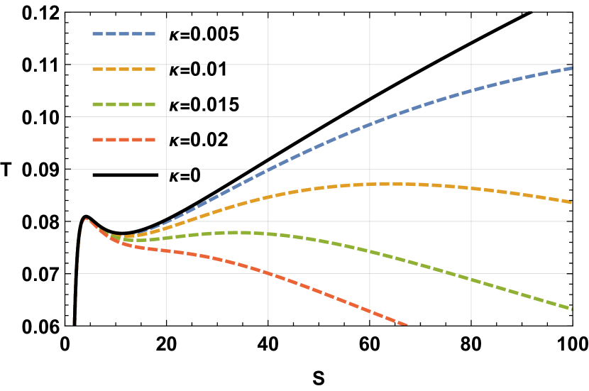
(a) J=0.2,Q=0.2,l=3.5

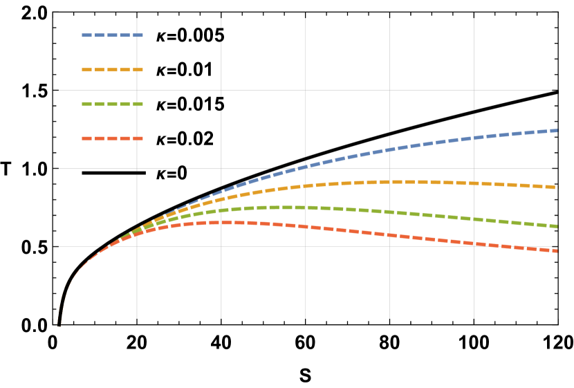
(b) J=0.5, Q=0.5, l=1

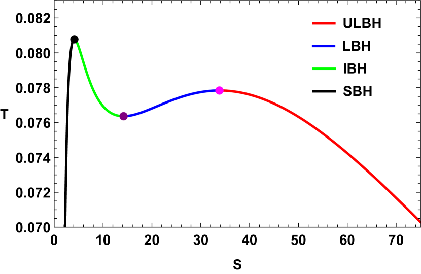
(c) J=0.2, Q=0.2, l=3.5, $\kappa$=0.015

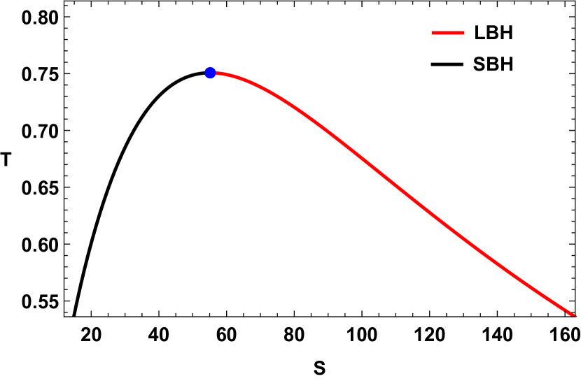
(d) J=0.5, Q=0.5, l=1, $\kappa$=0.015

Figure 18: Kerr-Sen-AdS black hole: T vs S plots for different values of $J,Q$ and $l.$ Here SBH, IBH, LBH, and ULBH represent small black holes, intermediate black holes, large black holes, and ultra-large black holes.

The specific heat $(C)$ of the Kerr-Sen-Ads black hole in KD statistics comes out to be :

$$C=\frac{\mathcal{M}}{\mathcal{N}}$$ (37)

Where,

$$\mathcal{M}=-(2(\kappa^{2}S^{2}+1)\sinh^{-1}(\kappa S)(\pi\kappa l^{2}+\sinh^{-1}(\kappa S))(4\pi^{3}\kappa^{3}J^{2}l^{2}+2\pi^{2}\kappa^{2}l^{2}Q^{2}\sinh^{-1}(\kappa S)+\pi\kappa l^{2}\sinh^{-1}(\kappa S)^{2}+\\ \sinh^{-1}(\kappa S)^{3})(4\pi^{4}\kappa^{4}J^{2}l^{4}-\pi^{2}\kappa^{2}l^{2}(l^{2}+2Q^{2})\sinh^{-1}(\kappa S)^{2}-4\pi\kappa l^{2}\sinh^{-1}(\kappa S)^{3}-3\sinh^{-1}(\kappa S)^{4})$$ (38)

and

$$\mathcal{N}=\kappa(6\pi^{2}\kappa^{2}l^{2}\sinh^{-1}(\kappa S)^{6}(-4\pi\kappa^{2}J^{2}S+l^{2}(\sqrt{\kappa^{2}S^{2}+1}-6\pi\kappa^{2}Q^{2}S)-2\pi\kappa^{2}l^{4}S+2Q^{2}\sqrt{\kappa^{2}S^{2}+1})\\ -2\pi^{3}\kappa^{3}l^{2}\sinh^{-1}(\kappa S)^{5}(l^{2}(12\pi\kappa^{2}l^{2}Q^{2}S+\pi\kappa^{2}l^{4}S-12Q^{2}\sqrt{\kappa^{2}S^{2}+1}+4\pi\kappa^{2}Q^{4}S)-24J^{2}(\sqrt{\kappa^{2}S^{2}+1}-\pi\kappa^{2}l^{2}S)t)\\ -\pi^{4}\kappa^{4}l^{4}\sinh^{-1}(\kappa S)^{4}(-8J^{2}\left(-3\pi\kappa^{2}l^{2}S-2\pi\kappa^{2}Q^{2}S+15\sqrt{\kappa^{2}S^{2}+1}\right)+l^{4}(4\pi\kappa^{2}Q^{2}S+\sqrt{\kappa^{2}S^{2}+1})+\\ l^{2}(8\pi\kappa^{2}Q^{4}S-12Q^{2}\sqrt{\kappa^{2}S^{2}+1})+4Q^{4}\sqrt{\kappa^{2}S^{2}+1})+8\pi^{6}\kappa^{6}J^{2}l^{6}\sinh^{-1}(\kappa S)^{2}(4\pi\kappa^{2}J^{2}S+l^{2}(2\pi\kappa^{2}Q^{2}S+3\sqrt{\kappa^{2}S^{2}+1})+\\ 6Q^{2}\sqrt{\kappa^{2}S^{2}+1})+32\pi^{7}\kappa^{7}J^{2}l^{6}\sinh^{-1}(\kappa S)(J^{2}(\pi\kappa^{2}l^{2}S+2\sqrt{\kappa^{2}S^{2}+1})+l^{2}Q^{2}\sqrt{\kappa^{2}S^{2}+1})+48\pi^{8}\kappa^{8}J^{4}l^{8}\sqrt{\kappa^{2}S^{2}+1}\\ +96\pi^{5}\kappa^{5}J^{2}l^{6}\sqrt{\kappa^{2}S^{2}+1}\sinh^{-1}(\kappa S)^{3}+8\pi\kappa l^{2}\sinh^{-1}(\kappa S)^{7}(-3\pi\kappa^{2}l^{2}S-2\pi\kappa^{2}Q^{2}S+\sqrt{\kappa^{2}S^{2}+1})+\\ (3\sqrt{\kappa^{2}S^{2}+1}-20\pi\kappa^{2}l^{2}S)\sinh^{-1}(\kappa S)^{8}-6\kappa S\sinh^{-1}(\kappa S)^{9})$$ (39)

Using equation eq.37, specific heat is plotted agaist KD entropy S while keeping $J=0.2,Q=0.2,l=3.5,\kappa=0.015$ fixed in FIG.19(a) and $J=0.5,Q=0.5,l=1,\kappa=0.015$ fixed in FIG.19(b). Dashed lines in both the figures represent the specific heat at GB statistics($\kappa=0$) for those particular sets of values. In FIG.19(a), there are three discontinuities for a non-zero $\kappa$ value. However, the dashed line indicates only two discontinuities for $\kappa=0$. This observation suggests that for the parameters $J=0.2$, $Q=0.2$, $l=3.5$, and $\kappa=0.015$, there are four branches. In contrast, for the case of GB statistics with $J=0.2$, $Q=0.2$, $l=3.5$, and $\kappa=0$, there are only three branches. Now coming to the stability of these black hole branches. Branches having a positive value of specific heat is thermally stable and vice versa. As the blue solid line in FIG.19(a) reveals the specific heat diverges at $S=4.1113,S=14.1983$ and $S=33.8221.$ Hence we detect that small black hole branch $(S<4.1113)$ and large black hole branch($14.1983<S<33.8221$) has positive specific heat, on the other hand, intermediate black hole branch ($4.1113<S<14.1983$) and ultra large black hole branch$(S>33.8221)$ has negative specific heat values. It can be inferred that SBH and LBH are thermally stable and IBH and ULBH are thermally unstable. The same is demonstarted in FIG.19(b) for the values $J=0.5,Q=0.5,l=1$ and $\kappa=0.015$. Here instead of four, only two black hole branches are visible. The small black hole branch($S<55.1569$) is seen to be thermally stable and the large black hole branch $S>55.1569$ is found to be thermally unstable. The dashed line shows $C$, in GB statistics which clearly indicates no phase transition for the chosen values of $J,Q$, and $l$.

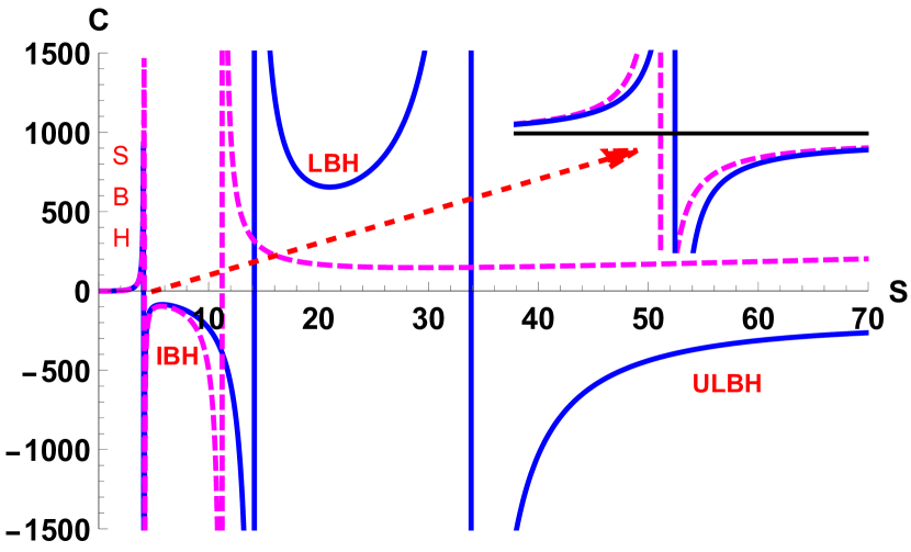
(a) C vs S plot($J=0.2,Q=0.2,\kappa=0.015$ and $l=3.5$

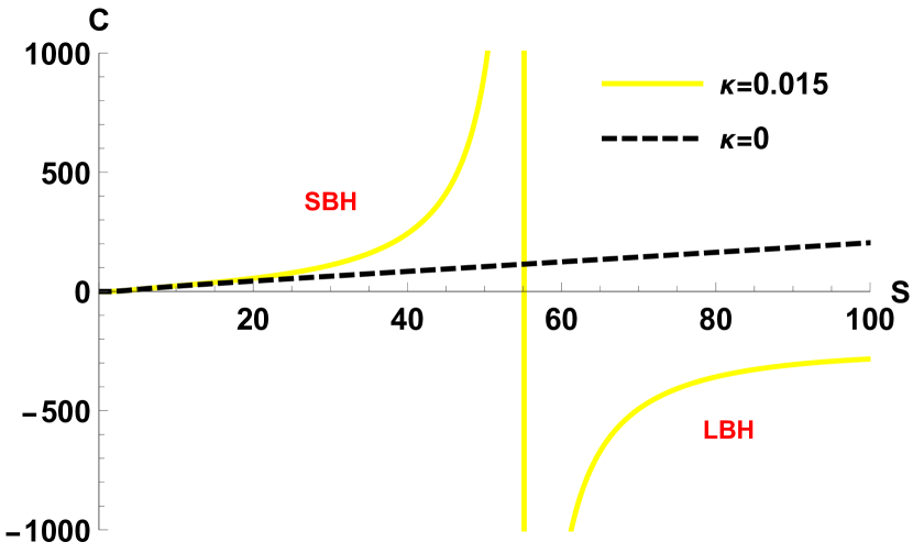
(b) (C vs S plot $J=0.5,Q=0.5,\kappa=0.015$ and $l=1$)

Figure 19: Kerr-Sen-AdS black hole: C vs S plots. Here SBH, IBH, LBH, and ULBH stand for small black hole branch, intermediate black hole branch, large black hole branch, ultra large black hole branch. The dashed line in both the figures suggests C vs S plot for $\kappa=0.$

Gibbs Free energy($F$)is calculated using the following relation:

$$F=M-TS=\frac{\mathcal{F}_{1}}{\mathcal{F}_{2}}$$ (40)

Where, T is the horizon temperature. $\mathcal{F}_{2},\mathcal{F}_{2}$ is obtained to be

$$\mathcal{F}_{1}=\frac{\kappa S\left(4\pi^{4}\kappa^{4}J^{2}l^{4}-\pi^{2}\kappa^{2}l^{2}\left(l^{2}+2Q^{2}\right)\sinh^{-1}(\kappa S)^{2}-4\pi\kappa l^{2}\sinh^{-1}(\kappa S)^{3}-3\sinh^{-1}(\kappa S)^{4}\right)}{\sqrt{\kappa^{2}S^{2}+1}}\\ +2\sinh^{-1}(\kappa S)\left(\pi\kappa l^{2}+\sinh^{-1}(\kappa S)\right)\left(4\pi^{3}\kappa^{3}J^{2}l^{2}+2\pi^{2}\kappa^{2}l^{2}Q^{2}\sinh^{-1}(\kappa S)+\pi\kappa l^{2}\sinh^{-1}(\kappa S)^{2}+\sinh^{-1}(\kappa S)^{3}\right)$$ (41)

And

$$\mathcal{F}_{2}=4\pi^{3/2}\kappa^{5}l^{2}\left(\frac{\sinh^{-1}(\kappa S)}{\kappa}\right)^{3/2}\sqrt{\pi l^{2}+\frac{\sinh^{-1}(\kappa S)}{\kappa}}\\ \sqrt{\frac{4\pi^{3}\kappa^{3}J^{2}l^{2}+2\pi^{2}\kappa^{2}l^{2}Q^{2}\sinh^{-1}(\kappa S)+\pi\kappa l^{2}\sinh^{-1}(\kappa S)^{2}+\sinh^{-1}(\kappa S)^{3}}{\kappa^{3}}}$$ (42)

FIG.20 is the free energy plot for two different sets of values of $J,Q,l$ and $\kappa$. For $J=0.2,Q=0.2,l=3.5$, there are four phases for different $\kappa$ values as shown in FIG.20(a) and for $J=0.5,Q=0.5,l=1$ there are only two phases for different $\kappa$ values. In FIG20(c), when $J=0.2,Q=0.2,l=3.5$ and $\kappa=0.015$ are taken, four phases are clearly visible where, black holes in the yellow region are the small black hole($S<4.1113$), black holes within the pink region are intermediate black holes($4.1113<S<14.1983$), black hole within the green region are large black hole($14.1983<S<33.8221$) and finally black holes in the blue region are ultra large black hole($S>33.8221$). On the other hand, when we use $J=0.5,Q=0.5,l=1$ and $\kappa=0.015$, we detect two black hole branches. Black holes in the yellow region are small black holes $(S<55.1569)$ and the black holes in the blue region are the large black holes($S>55.1569$).

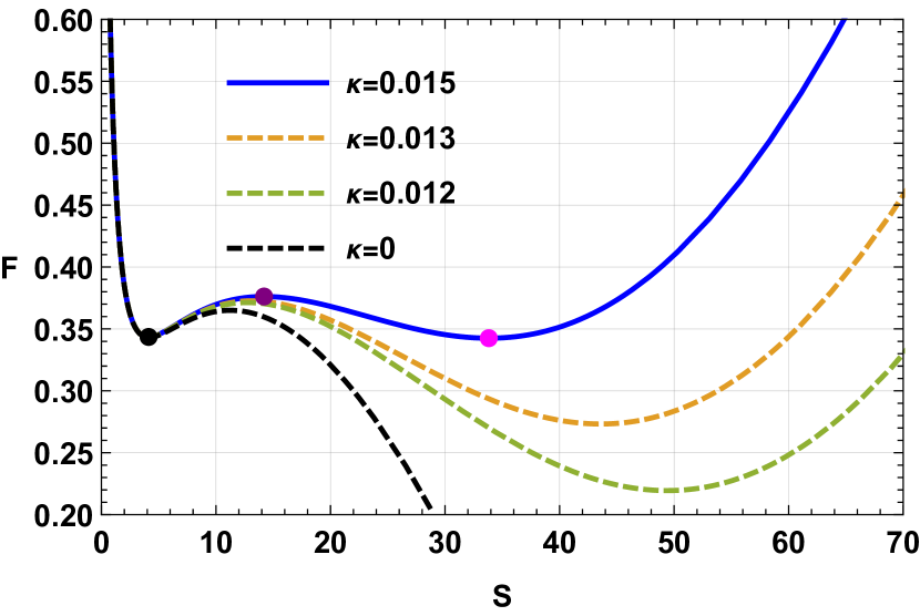
(a) F vs S plot at $J=0.2,Q=0.2,\kappa=0.015$ and $l=3.5$

(b) BH Phases in F vs S plot($J=0.2,Q=0.2,\kappa=0.015,l=3.5$)

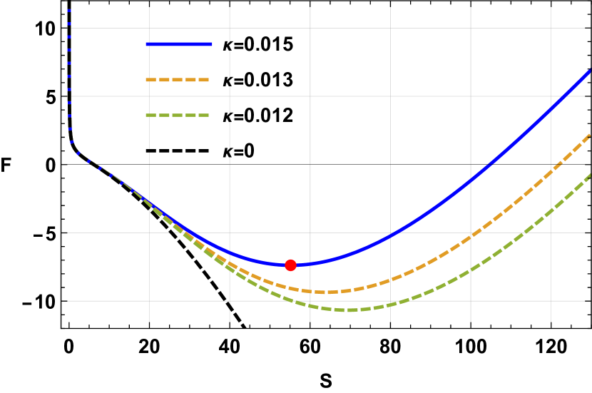
(c) F vs S plot at $J=0.5,Q=0.5,\kappa=0.015$ and $l=1$

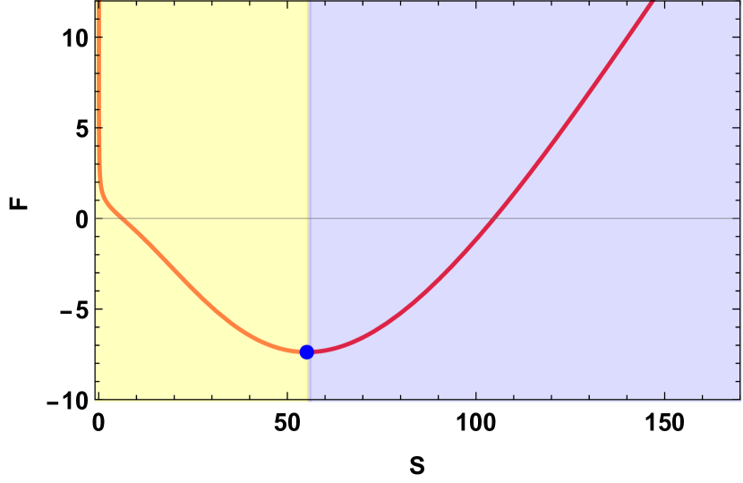
(d) BH Phases in F vs S plot($J=0.5,Q=0.5,\kappa=0.015,l=1$)

Figure 20: Kerr-Sen-AdS black hole: F vs S plots.

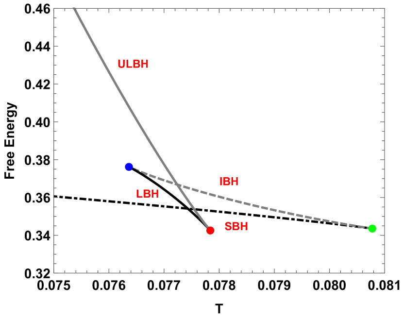
(a) F vs T plot at $J=0.2,Q=0.2,\kappa=0.015$ and $l=3.5$

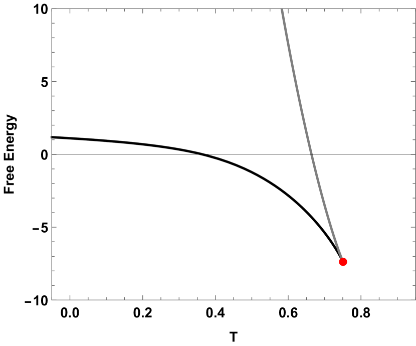
(b) F vs T plot at $J=0.5,Q=0.5,\kappa=0.015$ and $l=1$

Figure 21: Kerr- Sen-AdS black hole: F vs T plots.

To get some insight about the global and local stability of black holes, we construct the free energy landscape. To start with, we write the off shell free energy as :

$$F_{e}=F-T_{e}S=-\frac{2\pi^{3/2}l^{2}ST\sqrt{\frac{\sinh^{-1}(\kappa S)}{\kappa}}-\sqrt{\frac{\pi\kappa l^{2}+\sinh^{-1}(\kappa S)}{\kappa}}\sqrt{\frac{4\pi^{3}\kappa^{3}J^{2}l^{2}+2\pi^{2}\kappa^{2}l^{2}Q^{2}\sinh^{-1}(\kappa S)+\pi\kappa l^{2}\sinh^{-1}(\kappa S)^{2}+\sinh^{-1}(\kappa S)^{3}}{\kappa^{3}}}}{2\pi^{3/2}l^{2}\sqrt{\frac{\sinh^{-1}(\kappa S)}{\kappa}}}$$ (43)

Here $T_{e}$ is the ensemble temperature. The extremal points of the off-shell free energy represent a physical black hole and at the maximum value of off-shell free energy, the black hole is thermally unstable and vice versa. The free energy landscape for Kerr ads in KD statistics is plotted in the FIG.22. From the figures it can be inferred from FIG.7 that points $A,B,C,D,E$ are both thermally and globally stable, $K^{\prime},H,D_{3}$ are thermally stable but only locally stable, $K,G,H^{\prime}$ are thermally and locally unstable and finally $F,J,I,D_{2},L$ are both globally and thermally unstable.

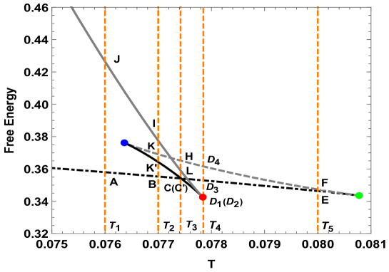
(a)

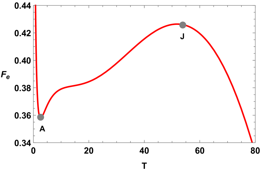
(b) $T_{e}=0.076$

(c) $T_{e}=0.077$

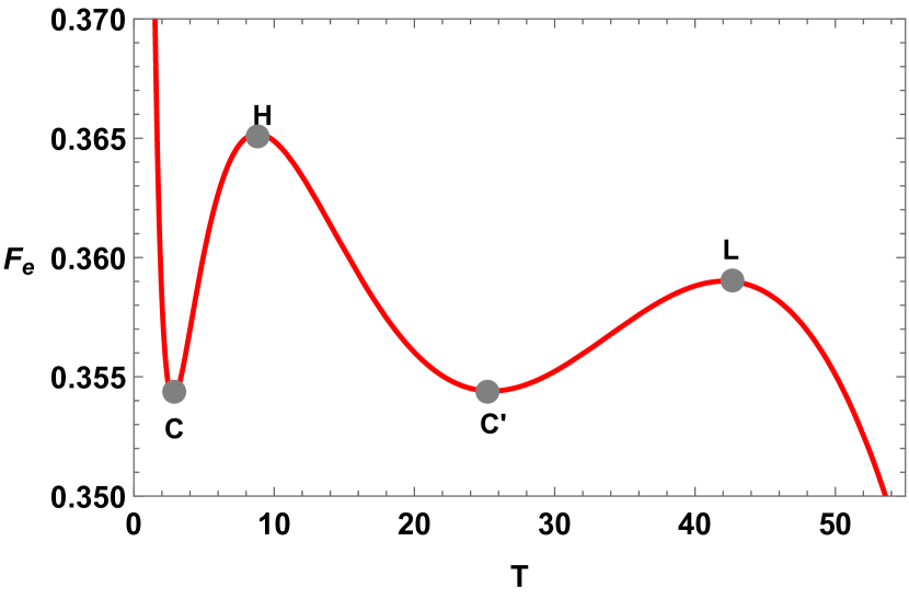
(d) $T_{e}=0.07742$

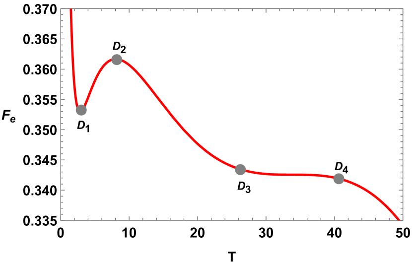
(e) $T_{e}=0.077838$

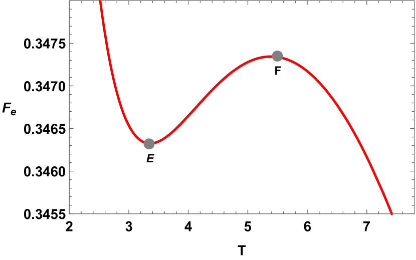
(f) $T_{e}=0.080$

Figure 22: Kerr-Sen-AdS black hole: Free energy landscape. For these plots, we have kept $J=0.2,Q=0.2,l=3.5$, and $\kappa=0.015$ fixed.

VI Thermodynamic Topology of Kerr-sen -Ads black hole

The off-shell free energy is constructed as :

$$\mathcal{F}=M-\frac{S}{\tau}\\ =-\frac{2\pi^{3/2}l^{2}S\sqrt{\frac{\sinh^{-1}(\kappa S)}{\kappa}}-\tau\sqrt{\frac{4\pi^{3}\kappa^{3}J^{2}l^{2}\left(\pi\kappa l^{2}+\sinh^{-1}(\kappa S)\right)+\left(\pi\kappa l^{2}\left(\pi\kappa Q^{2}+\sinh^{-1}(\kappa S)\right)+\sinh^{-1}(\kappa S)^{2}\right)^{2}}{\kappa^{4}}}}{2\pi^{3/2}l^{2}\tau\sqrt{\frac{\sinh^{-1}(\kappa S)}{\kappa}}}$$ (44)

The components of the vector $\phi$ are

$$\phi^{S} = \frac{\alpha_{2}}{\beta_{2}}$$ (45)

$$\phi^{\Theta} = -\cot\Theta~{}\csc\Theta.$$ (46)

where

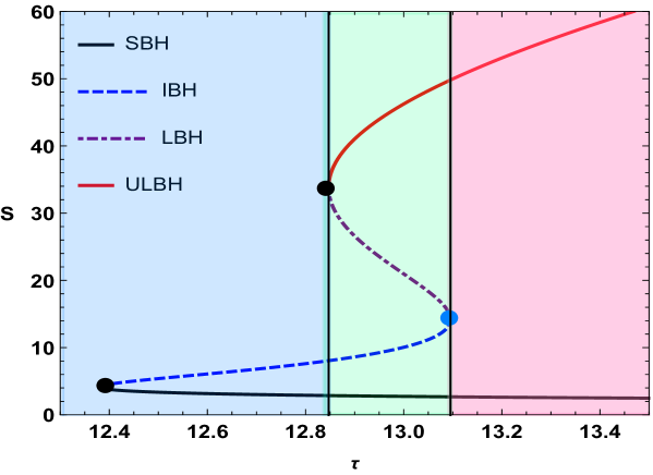
Figure 23: Kerr Sen Ads black hole : $\tau$ vs $S$ plot. Here we have taken $J=Q=0.2$ and $l=3.5$

$$\alpha_{2}=-4\pi^{4}\kappa^{4}J^{2}l^{4}\tau-4\pi^{3/2}\kappa^{4}l^{2}\sqrt{\kappa^{2}S^{2}+1}\left(\frac{\sinh^{-1}(\kappa S)}{\kappa}\right)^{3/2}\sqrt{\pi l^{2}+\frac{\sinh^{-1}(\kappa S)}{\kappa}}\\ \sqrt{\frac{4\pi^{3}\kappa^{3}J^{2}l^{2}+2\pi^{2}\kappa^{2}l^{2}Q^{2}\sinh^{-1}(\kappa S)+\pi\kappa l^{2}\sinh^{-1}(\kappa S)^{2}+\sinh^{-1}(\kappa S)^{3}}{\kappa^{3}}}\\ +\pi^{2}\kappa^{2}l^{2}\tau\left(l^{2}+2Q^{2}\right)\sinh^{-1}(\kappa S)^{2}+4\pi\kappa l^{2}\tau\sinh^{-1}(\kappa S)^{3}+3\tau\sinh^{-1}(\kappa S)^{4}$$ (47)

and

$$\beta_{2}=4\pi^{3/2}\kappa^{4}l^{2}\tau\sqrt{\kappa^{2}S^{2}+1}\left(\frac{\sinh^{-1}(\kappa S)}{\kappa}\right)^{3/2}\sqrt{\pi l^{2}+\frac{\sinh^{-1}(\kappa S)}{\kappa}}\\ \sqrt{\frac{4\pi^{3}\kappa^{3}J^{2}l^{2}+2\pi^{2}\kappa^{2}l^{2}Q^{2}\sinh^{-1}(\kappa S)+\pi\kappa l^{2}\sinh^{-1}(\kappa S)^{2}+\sinh^{-1}(\kappa S)^{3}}{\kappa^{3}}}$$ (48)

The expression for $\tau$ for which $\phi^{S}=0$, is calculated as:

$$\tau=\\ \frac{4\pi^{3/2}\kappa^{4}l^{2}\sqrt{\kappa^{2}S^{2}+1}\left(\frac{\sinh^{-1}(\kappa S)}{\kappa}\right)^{3/2}\sqrt{\frac{\pi\kappa l^{2}+\sinh^{-1}(\kappa S)}{\kappa}}\sqrt{\frac{4\pi^{3}\kappa^{3}J^{2}l^{2}+2\pi^{2}\kappa^{2}l^{2}Q^{2}\sinh^{-1}(\kappa S)+\pi\kappa l^{2}\sinh^{-1}(\kappa S)^{2}+\sinh^{-1}(\kappa S)^{3}}{\kappa^{3}}}}{-4\pi^{4}\kappa^{4}J^{2}l^{4}+2\pi^{2}\kappa^{2}l^{2}Q^{2}\sinh^{-1}(\kappa S)^{2}+\pi^{2}\kappa^{2}l^{4}\sinh^{-1}(\kappa S)^{2}+4\pi\kappa l^{2}\sinh^{-1}(\kappa S)^{3}+3\sinh^{-1}(\kappa S)^{4}}$$ (49)

Next, we present the plot of the KD entropy $S$ as a function of $\tau$ in Fig. 23 for the parameters $J=Q=0.2$, $l=3.5$, and $\kappa=0.0015$. This plot reveals four distinct branches of black holes. In Figs. 24(a), 24(b), 24(c), and 24(d), we provide vector plots illustrating the components $\phi^{S}$ and $\phi^{\Theta}$ with $\tau=13$. We identify zero points of the vector field at $S=2.7377$, $S=10.0419$, $S=20.9662$, and $S=46.2368$.

(a)

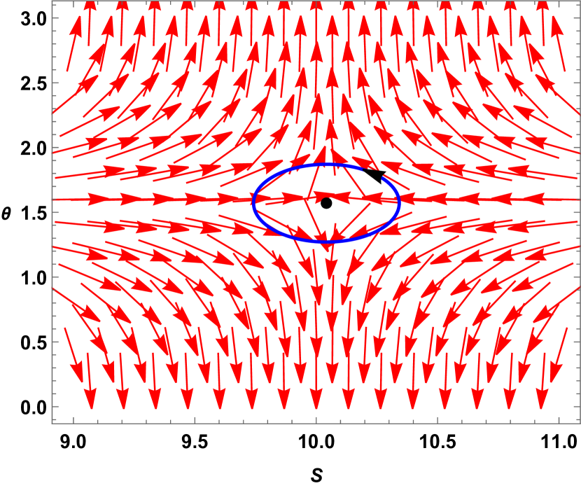
(b)

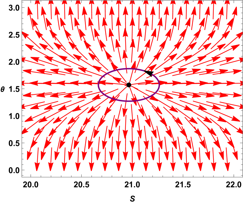
(c)

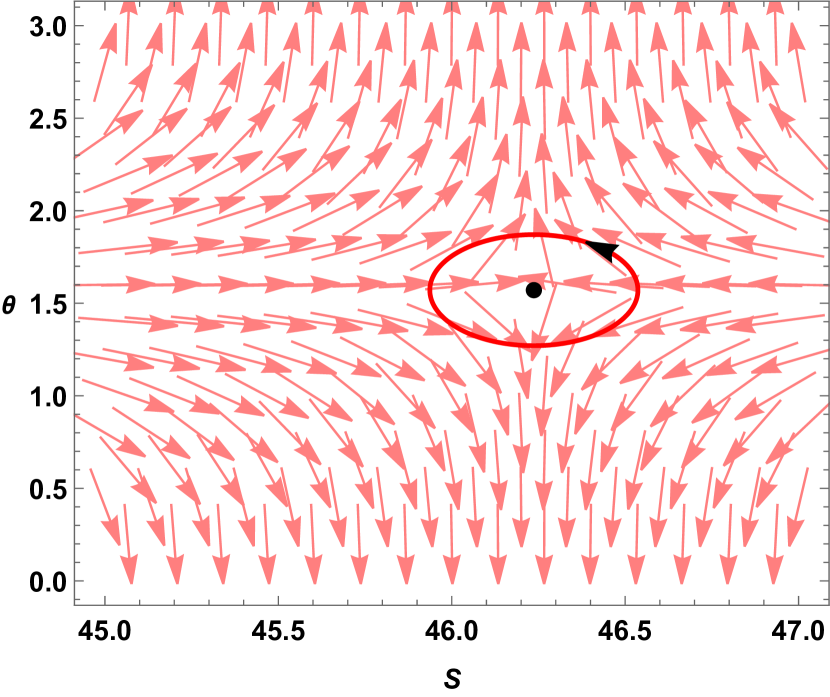
(d)

Figure 24: Kerr-Sen-Ads black holes: Vector plots of normalized ($\phi^{S}$,$\phi^{\Theta}$) field on the $S-\Theta$ plane

Fig. 25 presents four contour plots, each representing the computation of the winding number around these zero points. The colors in each figure correspond to the contours surrounding the zero points in the vector plots, indicating where the winding number is calculated. The winding number associated with $S=2.7377$ and $S=20.9662$ is $+1$, while that for $S=10.0419$ and $S=46.2368$ is $-1$. As the positive winding number suggests, the small and large black hole branches are stable. Conversely, the intermediate and ultra-large black hole branches are unstable as they have negative winding numbers. The total topological charge of the Kerr-Sen-AdS black hole in KD statistics is found to be $1-1+1-1=0$. Additionally, two annihilation points are observed at $(\tau_{c},S)=(12.3799,4.1193),(12.8470,33.8221)$, which is represented by black dots and one generation point is observed at $(\tau_{c},S)=(13.0952,14.1983)$ represented by a blue dot in Fig. 23.

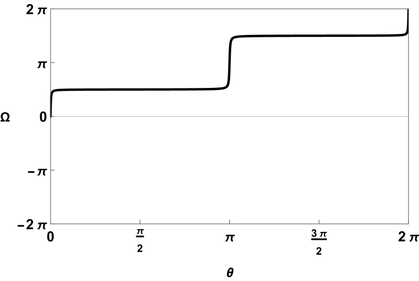
(a)

(b)

(c)

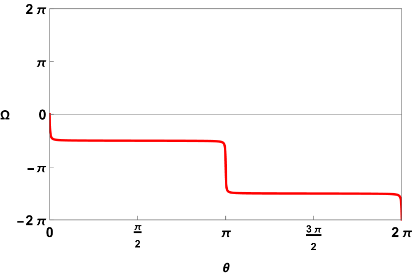
(d)

Figure 25: Kerr-Sen-Ads black holes: Winding number calculations for Kerr-Sen-Ads black holes. The black solid line in Fig.25(a) and puple dot dashed line in Fig.25(c) represents winding number for SBH and LBH respectively which equals to $+1$ and the blue solid line in Fig.25(b). Red solid line in Fig.25(d) represents winding number for IBH and ULBH respectively which euals to $-1.$

Another case is presented in Fig.26, where we see two black hole branches in Fig.26(a): a small black hole branch(SBH) and a large black hole branch (LBH). The winding number for SBH is $+1$ which means it is stable and that for LBH is found to be $-1$ which suggests it is an unstable branch. Moreover we found a annihilation point in $(\tau=1.33207,S=55.1569)$ represented by the black dot in the Fig.26(a)

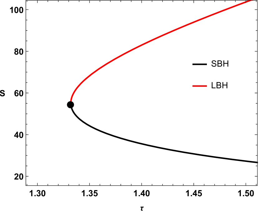
(a)

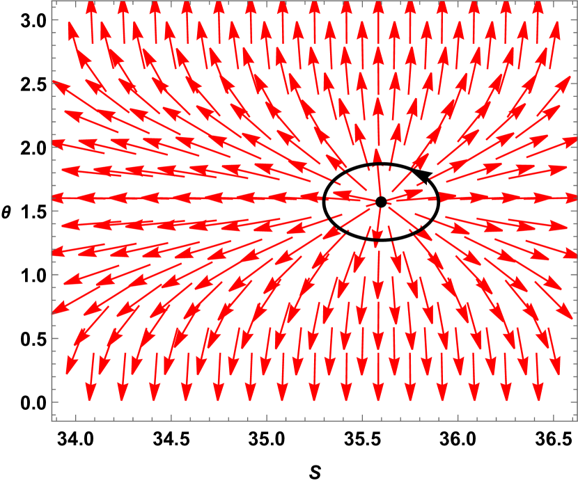
(b)

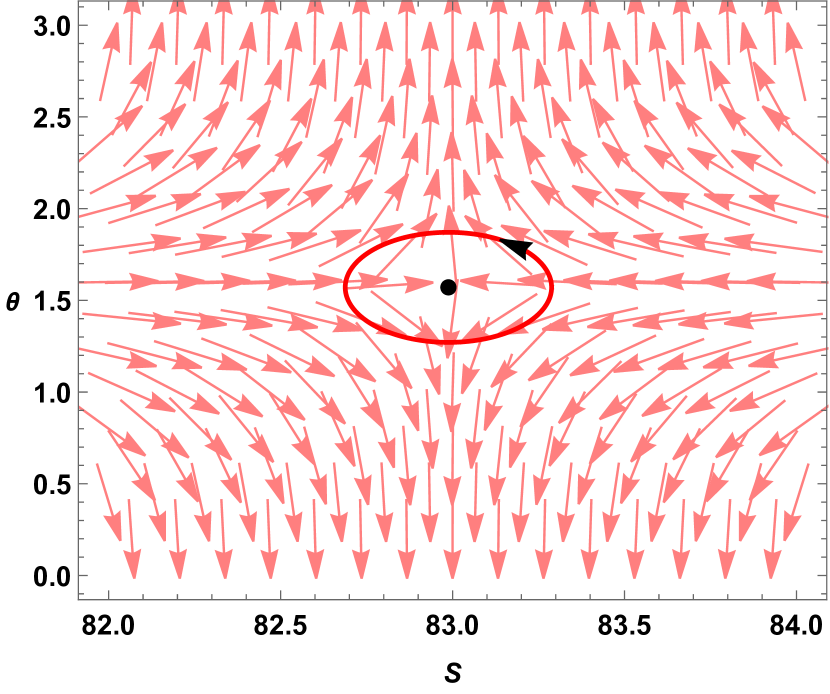
(c)

(d)

Figure 26: Kerr-Sen-Ads black holes: In Fig.26(a), $\tau$ vs $S$ is plotted for Kerr-Sen-Ads black holes when $J=Q=0.5,l=1$ and $\kappa=0.015$ is taken. In Fig.26(b) and Fig.26(c) vectorplots are shown in $S-\theta$ plane where the zero point (S,$\theta$)= $(35.5982,\pi/2)$ in Fig.26(b) is on the SBH and the zero point (S,$\theta$)= $(82.9878,\pi/2)$ in Fig.26(c) is on the LBH. The winding number calculation is shown in Fig.26(d) where the black solid line in Fig.26(d) represents winding number for SBH which equals to $+1$ and the red solid line in Fig.26(d) represents winding number for LBH which euals to $-1.$

The number of branches in the $\tau$ vs $S$ graph changes with a change in the value of $J,Q$ and $l.$ We observe either four or two branches depending on the values of thermodynamic parameters. However, the topological charge remains invariant when the values of $J,Q,l$ and $\kappa$ are varied. Here again, we see a change in the topological charge of Kerr-Sen Ads black hole when we change the framework from GB statistics to KD statistics. In GB statistics, the topological charge of the black hole is $+1$ and the same for the black hole is found to be $0$ in KD statistics formalism.
In Fig. 27(a) and Fig. 27(b), we show the variation of $\kappa$ with $J=Q=0.2$, $l=3.5$, and with $J=Q=0.5$, $l=1$, respectively. Fig. 27(c) illustrates the variation of $J$ with $Q=0.2$, $l=3.5$, and $\kappa=0.015$ held constant. Fig. 27(d) demonstrates the variation of $Q$ while keeping $J=0.2$, $l=3.5$, and $\kappa=0.015$ fixed. Additionally, in Fig. 27(e), we depict the variation of $l$ with $Q=J=0.2$ and $\kappa=0.015$ fixed.

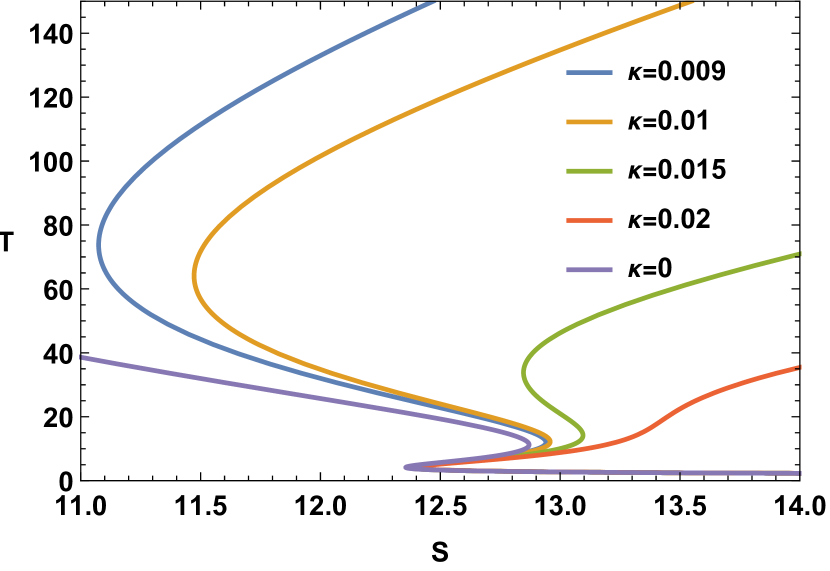
(a)

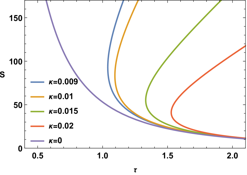
(b)

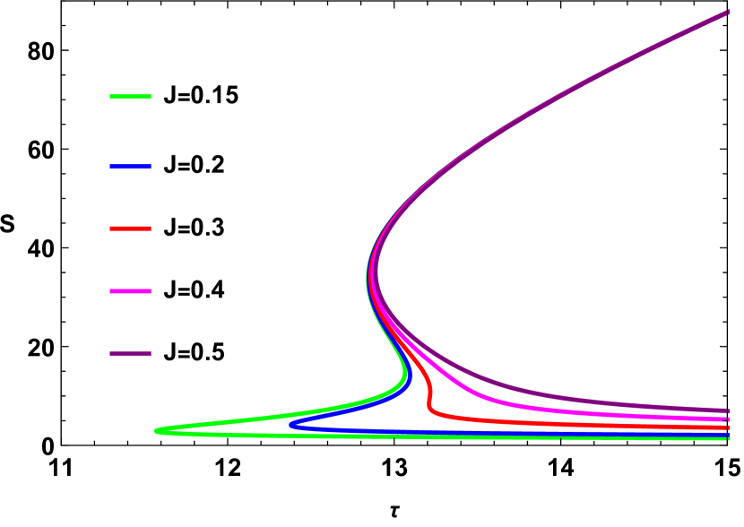
(c)

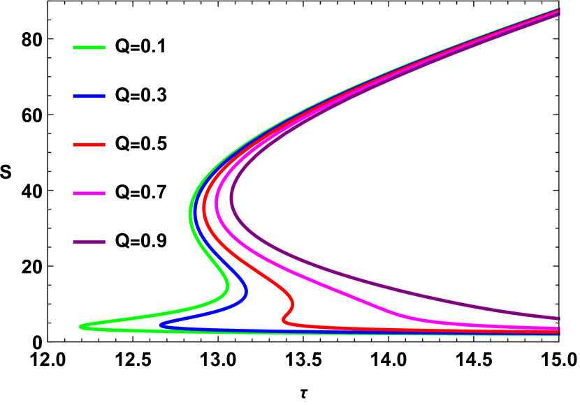
(d)

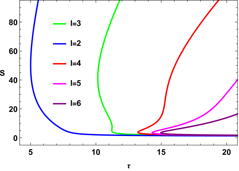
(e)

Figure 27: Variations of $\tau$ vs $S$ plots for kerr-sen-ads black holes with different thermodynamic parameters

In conclusion, for the Kerr-Sen-ads black hole in KD statistics, the topological charge is $0$ and it is observed that, the topological charge is independent of other thermodynamic parameters.

VII Thermodynamic geometry of Kerr-Sen-AdS black holes

The line element for the Ruppeiner metric in the Kerr-Sen-AdS black hole could be written as :

$$dS_{R}^{2}=\frac{1}{T}\left(\frac{\partial^{2}M}{\partial S^{2}}dS^{2}+\frac{\partial^{2}M}{\partial J^{2}}dJ^{2}+\frac{\partial^{2}M}{\partial Q^{2}}dQ^{2}+2\frac{\partial^{2}M}{\partial S\partial J}dSdJ+2\frac{\partial^{2}M}{\partial J\partial Q}dJdQ+2\frac{\partial^{2}M}{\partial S\partial Q}dSdQ\right)$$

and the line element for the GTD metric in the Kerr-Sen-AdS black hole is given by:

$$dS_{G}^{2}=S\left(\frac{\partial M}{\partial S}\right)\left(-\frac{\partial^{2}M}{\partial S^{2}}dS^{2}+\frac{\partial^{2}M}{\partial J^{2}}dJ^{2}+\frac{\partial^{2}M}{\partial Q^{2}}dQ^{2}\right)$$

We see from Fig.28(b) that the Ruppeiner scalar is plotted against the Kaniadakis entropy for $J=Q=0.2$ and $L=3.5$ which has three singularities at $S=1.193,16.184$ and $33.297$ for $\kappa=0.015$ whereas in Fig.29(b) we see that for $J=Q=0.5$ and $L=1$ there is only one singularity at $S=55.100$ for $\kappa=0.015$. The GTD scalar on the other hand has singularities at $S=4.119,14.200$ and $33.822$ for $J=Q=0.2$ and $L=3.5$ as can be seen in Fig.30(b). We see from Fig.31(b) that for $J=Q=0.5$ and $L=1$ there is only one singularity at $S=55.157$. It is worth mentioning that unlike Ruppeiner scalar it is only the GTD scalar that produce singularities which agree with the points of Davies type phase transitions found in the heat capacity curves.

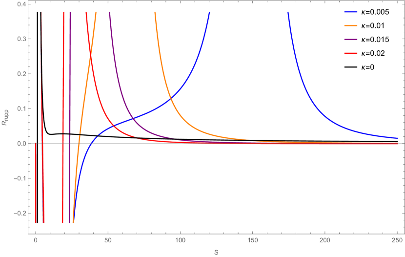
(a) For all $\kappa$

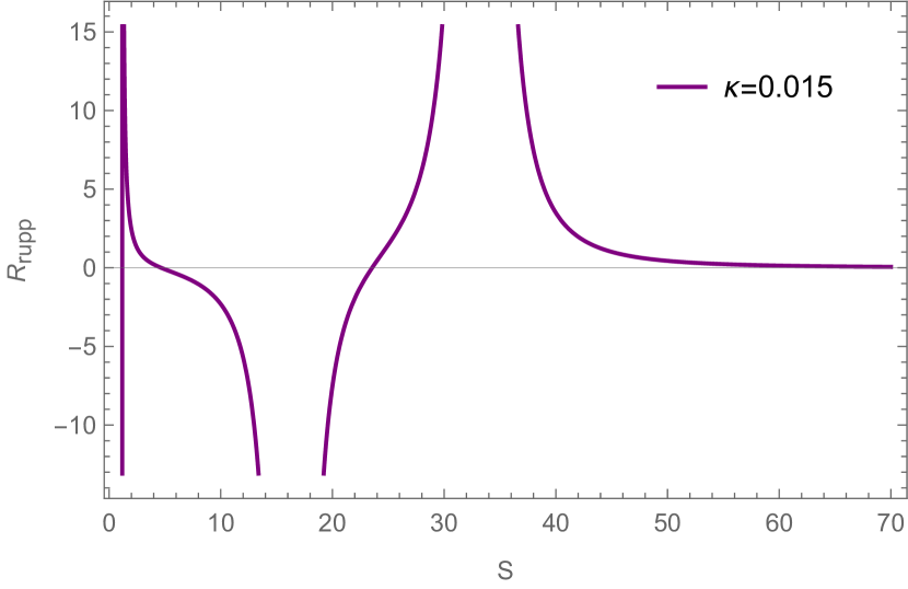
(b) For $\kappa=0.015$

Figure 28: The Ruppeiner scalar versus Entropy plot for Kerr-Sen-AdS black hole for $J=Q=0.2$ and $L=3.5$.

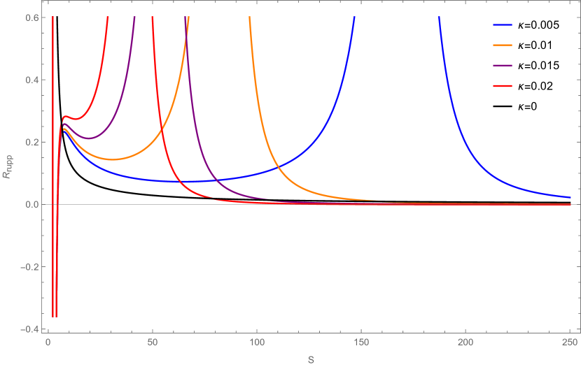
(a) For all $\kappa$

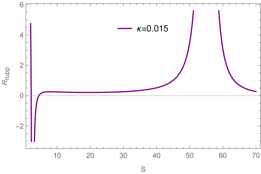
(b) For $\kappa=0.015$

Figure 29: The Ruppeiner scalar versus Entropy plot for Kerr-Sen-AdS black hole for $J=Q=0.5$ and $L=1$.

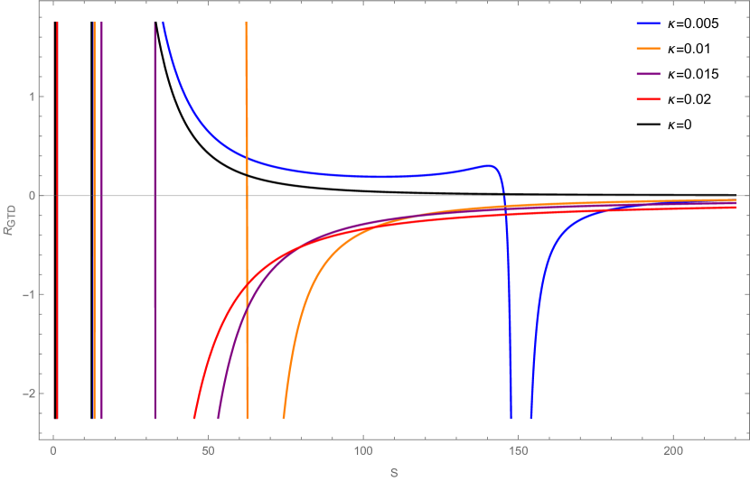
(a) For all $\kappa$

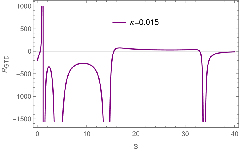
(b) For $\kappa=0.015$

Figure 30: The GTD scalar versus Entropy plot for Kerr-Sen-AdS black hole for $J=Q=0.2$ and $L=3.5$.

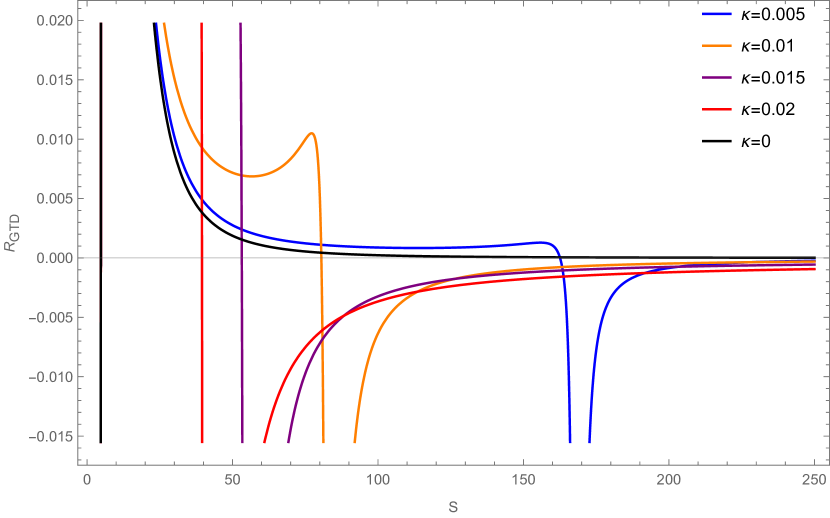
(a) For all $\kappa$

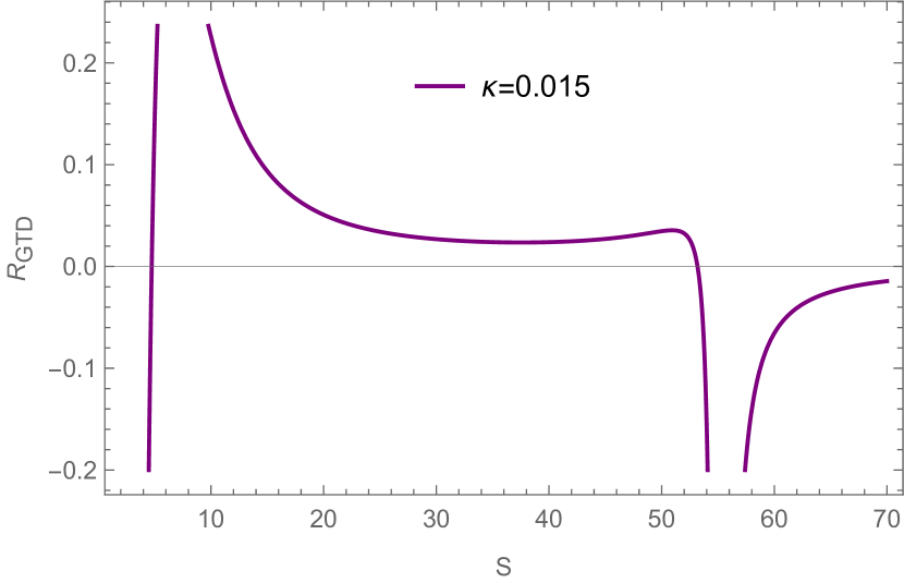
(b) For $\kappa=0.015$

Figure 31: The GTD scalar versus Entropy plot for Kerr-Sen-AdS black hole for $J=Q=0.5$ and $L=1$.

VIII Thermodynamics of Kerr-Newman-Ads Black holes

The ADM mass of the Kerr-Newman-Ads black hole in terms of entropy is obtained to be

$$M=\frac{\sqrt{4\pi^{3}J^{2}l^{2}\left(\pi l^{2}+S\right)+\left(\pi l^{2}\left(\pi Q^{2}+S\right)+S^{2}\right)^{2}}}{2\pi^{3/2}l^{2}\sqrt{S}}$$ (50)

In KD statistics the mass is converted to the KD mass as :

$$M_{KD}=\frac{\sqrt{\frac{4\pi^{3}\kappa^{3}J^{2}l^{2}\left(\pi\kappa l^{2}+\sinh^{-1}(\kappa S)\right)+\left(\pi\kappa l^{2}\left(\pi\kappa Q^{2}+\sinh^{-1}(\kappa S)\right)+\sinh^{-1}(\kappa S)^{2}\right)^{2}}{\kappa^{4}}}}{2\pi^{3/2}l^{2}\sqrt{\frac{\sinh^{-1}(\kappa S)}{\kappa}}}$$ (51)

The other thermodynamic quantities are obtained as :

$$\text{Temperature :}\hskip 28.45274ptT=\\ \frac{\pi^{4}\kappa^{4}\left(-l^{4}\right)\left(4J^{2}+Q^{4}\right)+\pi^{2}\kappa^{2}l^{2}\left(l^{2}+2Q^{2}\right)\sinh^{-1}(\kappa S)^{2}+4\pi\kappa l^{2}\sinh^{-1}(\kappa S)^{3}+3\sinh^{-1}(\kappa S)^{4}}{4\pi^{3/2}\kappa^{4}l^{2}\sqrt{\kappa^{2}S^{2}+1}\left(\frac{\sinh^{-1}(\kappa S)}{\kappa}\right)^{3/2}\sqrt{\frac{4\pi^{3}\kappa^{3}J^{2}l^{2}\left(\pi\kappa l^{2}+\sinh^{-1}(\kappa S)\right)+\left(\pi\kappa l^{2}\left(\pi\kappa Q^{2}+\sinh^{-1}(\kappa S)\right)+\sinh^{-1}(\kappa S)^{2}\right)^{2}}{\kappa^{4}}}}$$ (52)

$$\text{Specific heat :}\hskip 28.45274ptC=\frac{\mathcal{X}}{\mathcal{Y}}$$ (53)

Where,

$$\mathcal{X}=-2(\kappa^{2}S^{2}+1)\sinh^{-1}(\kappa S)(\pi^{4}\kappa^{4}l^{4}(4J^{2}+Q^{4})-\pi^{2}\kappa^{2}l^{2}(l^{2}+2Q^{2})\sinh^{-1}(\kappa S)^{2}-4\pi\kappa l^{2}\sinh^{-1}(\kappa S)^{3}\\ -3\sinh^{-1}(\kappa S)^{4})(\pi^{4}\kappa^{4}l^{4}(4J^{2}+Q^{4})+2\pi^{3}\kappa^{3}l^{2}(2J^{2}+l^{2}Q^{2})\sinh^{-1}(\kappa S)+\pi^{2}\kappa^{2}l^{2}(l^{2}+2Q^{2})\sinh^{-1}(\kappa S)^{2}\\ +2\pi\kappa l^{2}\sinh^{-1}(\kappa S)^{3}+\sinh^{-1}(\kappa S)^{4})$$ (54)

and

$$\mathcal{Y}=\kappa(3\pi^{8}\kappa^{8}l^{8}(4J^{2}+Q^{4})^{2}\sqrt{\kappa^{2}S^{2}+1}+24\pi^{5}\kappa^{5}l^{6}(4J^{2}+Q^{4})\sqrt{\kappa^{2}S^{2}+1}\sinh^{-1}(\kappa S)^{3}\\ +2\pi^{7}\kappa^{7}l^{6}(4J^{2}+Q^{4})\sinh^{-1}(\kappa S)(4J^{2}(\pi\kappa^{2}l^{2}S+2\sqrt{\kappa^{2}S^{2}+1})+l^{2}Q^{2}(\pi\kappa^{2}Q^{2}S+4\sqrt{\kappa^{2}S^{2}+1}))\\ +2\pi^{6}\kappa^{6}l^{6}(4J^{2}+Q^{4})\sinh^{-1}(\kappa S)^{2}(4\pi\kappa^{2}J^{2}S+l^{2}(2\pi\kappa^{2}Q^{2}S+3\sqrt{\kappa^{2}S^{2}+1})\\ +6Q^{2}\sqrt{\kappa^{2}S^{2}+1}))+6\pi^{2}\kappa^{2}l^{2}\sinh^{-1}(\kappa S)^{6}(-4\pi\kappa^{2}J^{2}S-2\pi\kappa^{2}l^{4}S+l^{2}(\sqrt{\kappa^{2}S^{2}+1}-6\pi\kappa^{2}Q^{2}S)+2Q^{2}\sqrt{\kappa^{2}S^{2}+1}))\\ -\pi^{4}\kappa^{4}l^{4}\sinh^{-1}(\kappa S)^{4}(-8J^{2}(-3\pi\kappa^{2}l^{2}S-2\pi\kappa^{2}Q^{2}S+15\sqrt{\kappa^{2}S^{2}+1})+l^{4}(4\pi\kappa^{2}Q^{2}S+\sqrt{\kappa^{2}S^{2}+1})+12l^{2}Q^{2}(\pi\kappa^{2}Q^{2}S-\sqrt{\kappa^{2}S^{2}+1})\\ -18Q^{4}\sqrt{\kappa^{2}S^{2}+1}))-2\pi^{3}\kappa^{3}l^{2}\sinh^{-1}(\kappa S)^{5}(l^{2}(\pi\kappa^{2}l^{4}S+12\pi\kappa^{2}l^{2}Q^{2}S+6\pi\kappa^{2}Q^{4}S-12Q^{2}\sqrt{\kappa^{2}S^{2}+1})-24J^{2}(\sqrt{\kappa^{2}S^{2}+1}-\pi\kappa^{2}l^{2}S))\\ +8\pi\kappa l^{2}\sinh^{-1}(\kappa S)^{7}(-3\pi\kappa^{2}l^{2}S-2\pi\kappa^{2}Q^{2}S+\sqrt{\kappa^{2}S^{2}+1}))+(3\sqrt{\kappa^{2}S^{2}+1}-20\pi\kappa^{2}l^{2}S)\sinh^{-1}(\kappa S)^{8}-6\kappa S\sinh^{-1}(\kappa S)^{9})$$ (55)

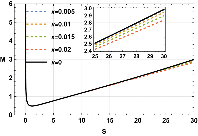
(a) J=0.2, Q=0.2, l=3.5

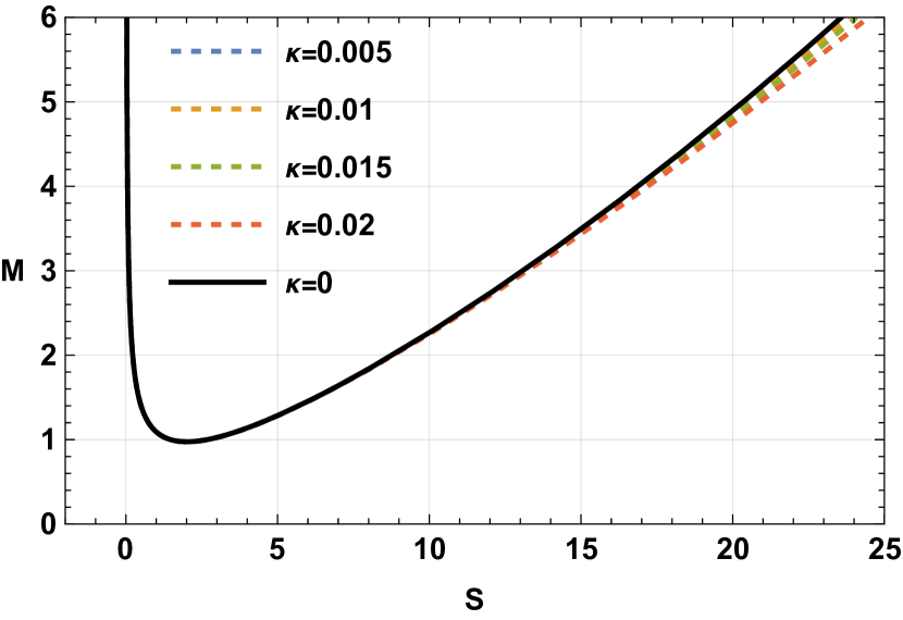
(b) J=0.5, Q=0.5, l=1

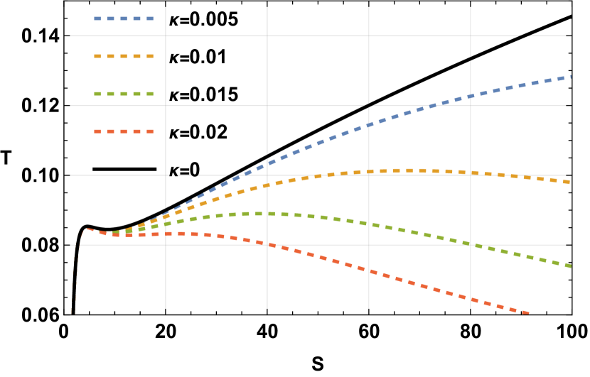
(c) J=0.2,Q=0.2,l=3.5

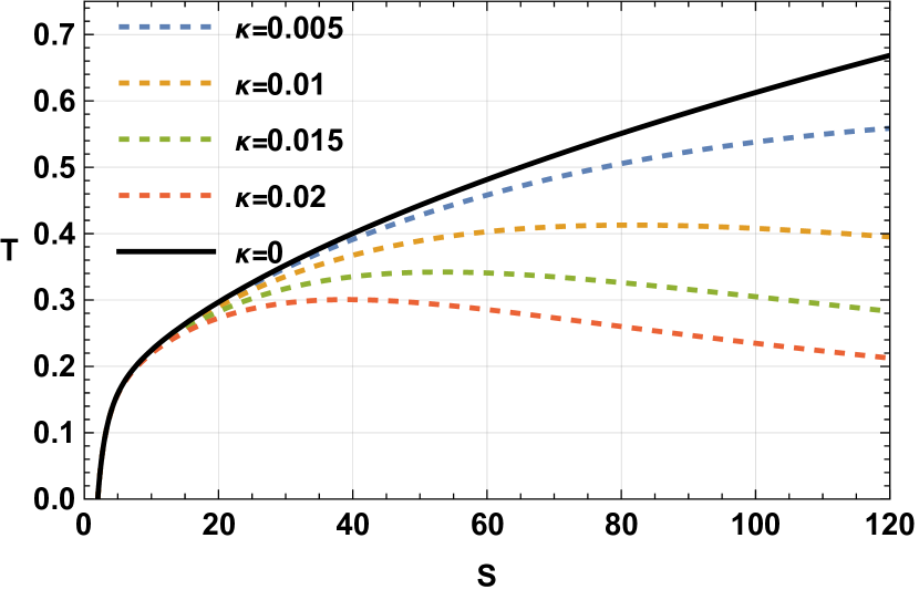
(d) J=0.5, Q=0.5, l=1

Figure 32: Kerr-Newman-AdS black hole: Figure (a) and (b) represents $M$ vs $S$ plot for different value of $\kappa,J,Q$ and $l.$ The impact of $\kappa$ parameter is more visible with higher values of $S$. Figure (c) and (d) represents temperature $T$ vs $S$ plot for different value of $\kappa,J,Q$ and $l.$

In a manner consistent with previous cases, the impact of the KD parameter $\kappa$ on the black hole mass and temperature becomes increasingly pronounced at higher values of KD entropy $S$. Figures 32(a) and 32(b) illustrate the KD mass of the black hole in KD statistics for various $\kappa$ values, with parameters fixed at $J=0.2$, $Q=0.2$, $l=3.2$ in Fig. 32(a) and $J=0.5$, $Q=0.5$, $l=1$ in Fig. 32(b). Figure 32(c) presents the temperature $T$ as a function of entropy $S$, highlighting two types of phase transitions in Kerr-Newman-AdS black holes. For $J=0.2$, $Q=0.2$, and $l=3.2$, shown in Fig. 32(c), four distinct black hole phases are observed. The black solid line represents the phase transition in GB statistics. In contrast, Fig. 32(d) shows $J=0.5$, $Q=0.5$, and $l=1.5$, where only two black hole branches are detected, with no phase transition in GB statistics, as depicted by the black solid line.Figure 33 provides a detailed view of these phase transition phenomena. In Fig. 33(a), with parameters $J=0.2$, $Q=0.2$, $l=3.2$, and $\kappa=0.015$, we identify four black hole branches: a small black hole branch (SBH) for $S<4.5450$ (up to the black dot), an intermediate black hole branch (IBH) for $4.5450<S<10.0505$ (up to the purple dot), a large black hole branch (LBH) for $10.0505<S<38.6597$ (up to the magenta dot), and an ultra-large black hole branch (ULBH) for $S>38.6597$ (beyond the red dot). Altering $J$, $Q$, and $l$ slightly can reduce the number of branches from four to two, as illustrated in Fig. 33(b). For instance, with $J=0.5$, $Q=0.5$, $l=1.5$, and $\kappa=0.015$, we observe only two branches: an LBH branch for $S<53.2136$ (blue dot) and an SBH branch for $S>53.2136$. Figures 33(c) and 33(d) display 3D plots with temperature $T$, entropy $S$, and $l$ as the three axes.

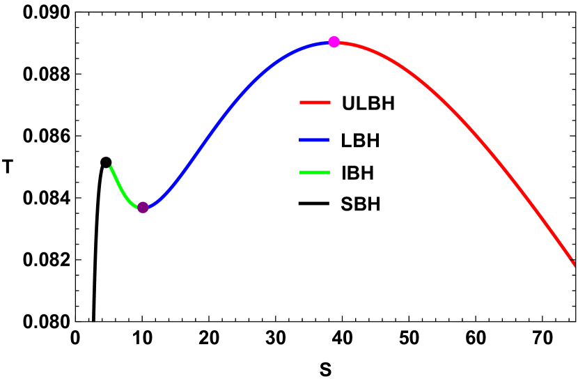
(a) J=0.2, Q=0.2, l=3.5, $\kappa$=0.015 and $l=3.2$

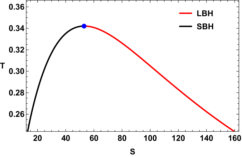
(b) J=0.5, Q=0.5, l=1, $\kappa$=0.015 and $l=1.5$

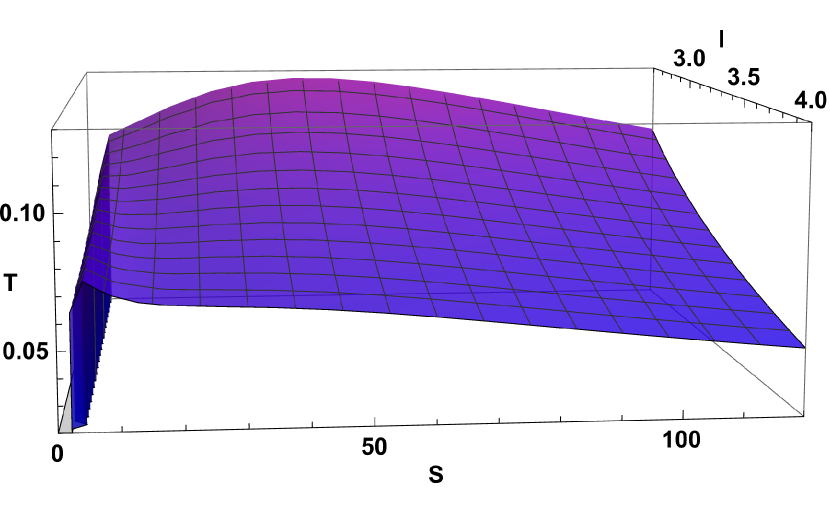
(c) C vs S plot($J=0.2,Q=0.2,\kappa=0.015$ and $l=3.2$

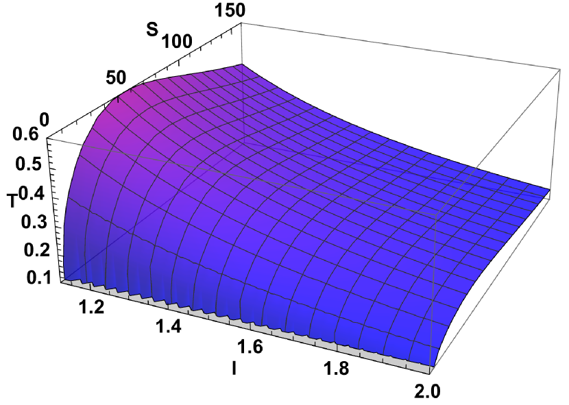
(d) (C vs S plot $J=0.5,Q=0.5,\kappa=0.015$ and $l=1.5$)

Figure 33: Kerr-Newman-AdS black hole: T vs S plots for different values of $J,Q$ and $l.$ Here SBH, IBH, LBH, and ULBH represent small black holes, intermediate black holes, large black holes, and ultra-large black holes.

In FIG.34(a) and FIG.34(b), specific heat is plotted against KD entropy S using equation eq.53, for the set of values $J=0.2,Q=0.2,l=3.2,\kappa=0.015$ and $J=0.5,Q=0.5,l=1.5,\kappa=0.015$ respectively. Dashed lines in both the figures represent the specific heat at GB statistics($\kappa=0$) for those particular sets of values. The locations of the discontinuities in these plots exactly matches with the phase transitioning point observed in the respective $T$ vs $S$ plots.Again,it can be inferred from FIG.34(a) that SBH and LBH are thermally stable and IBH and ULBH are thermally unstable. The same is demonstrated in FIG.34(b) where the small black hole branch is seen to be thermally stable and the large black hole branch is found to be thermally unstable. In FIG.34(c) and FIG.34(d), 3 D plots are shown for better representation.

(a) J=0.2, Q=0.2, l=3.2

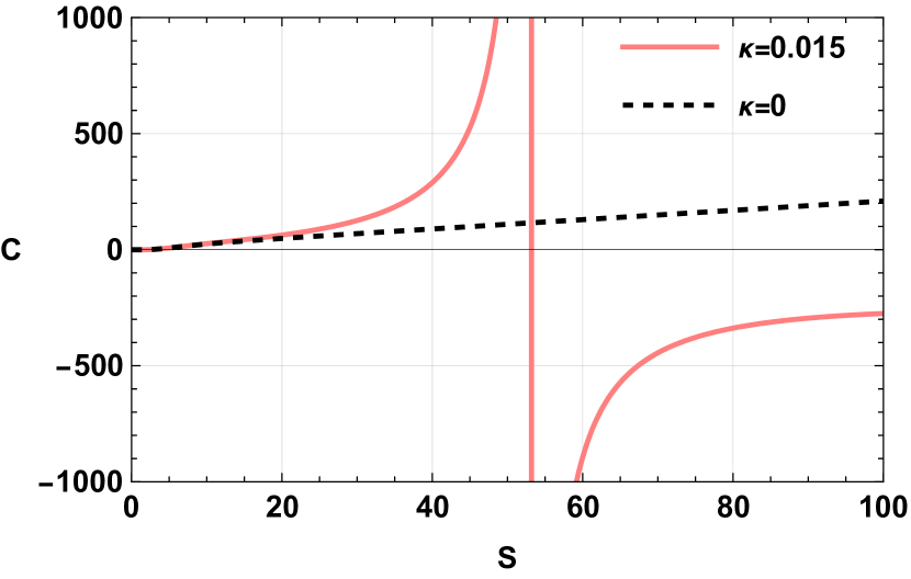
(b) J=0.5, Q=0.5, l=1.5

(c) J=0.2,Q=0.2,l=3.2

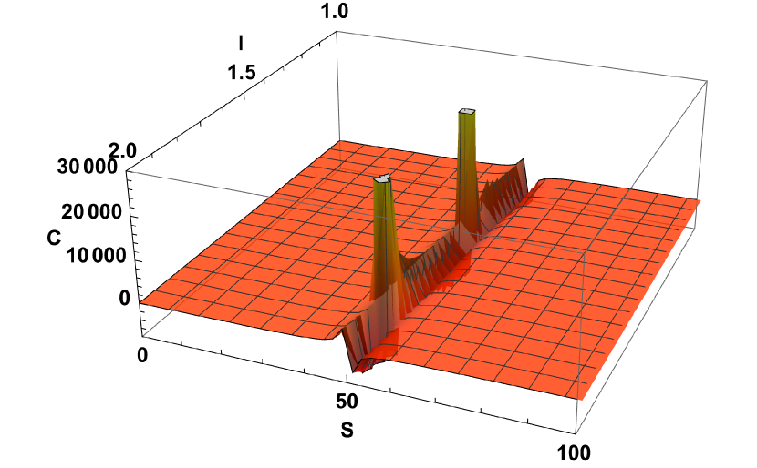
(d) J=0.5, Q=0.5, l=1.5

Figure 34: Kerr-Newman-AdS black hole: Figure (a) and (b) represents $C$ vs $S$ plot for different value of $\kappa,J,Q$ and $l.$ Figure (c) and (d) represents 3D plot of specific heat.

Gibbs Free energy($F$)is calculated using the following relation:

$$F=M-TS=\frac{\mathcal{F}_{3}}{\mathcal{F}_{4}}$$ (56)

Where, T is the horizon temperature. $\mathcal{F}_{3}\mathcal{F}_{4}$ is obtained to be

$$\mathcal{F}_{3}=2\sqrt{\kappa^{2}S^{2}+1}\sinh^{-1}(\kappa S)\left(4\pi^{3}\kappa^{3}J^{2}l^{2}\left(\pi\kappa l^{2}+\sinh^{-1}(\kappa S)\right)+\left(\pi\kappa l^{2}\left(\pi\kappa Q^{2}+\sinh^{-1}(\kappa S)\right)+\sinh^{-1}(\kappa S)^{2}\right)^{2}\right)\\ +\kappa S\left(\pi^{4}\kappa^{4}l^{4}\left(4J^{2}+Q^{4}\right)-\pi^{2}\kappa^{2}l^{2}\left(l^{2}+2Q^{2}\right)\sinh^{-1}(\kappa S)^{2}-4\pi\kappa l^{2}\sinh^{-1}(\kappa S)^{3}-3\sinh^{-1}(\kappa S)^{4}\right)$$ (57)

And

$$\mathcal{F}_{4}=4\pi^{3/2}\kappa^{5}l^{2}\sqrt{\kappa^{2}S^{2}+1}\left(\frac{\sinh^{-1}(\kappa S)}{\kappa}\right)^{3/2}\\ \sqrt{\frac{4\pi^{3}\kappa^{3}J^{2}l^{2}\left(\pi\kappa l^{2}+\sinh^{-1}(\kappa S)\right)+\left(\pi\kappa l^{2}\left(\pi\kappa Q^{2}+\sinh^{-1}(\kappa S)\right)+\sinh^{-1}(\kappa S)^{2}\right)^{2}}{\kappa^{4}}}$$ (58)

FIG.35 is the free energy F vs S plot for Kerr-Newman AdS black hole. In FIG.36, parametric plot between temperature T and free energy F is shown for two different set of values. In FIG.36(a) we have considered $J=0.2,Q=0.2,\kappa=0.015,l=3.2$ and in FIG.36(b) we have taken $J=0.5,Q=0.5,\kappa=0.015,l=1.5$.

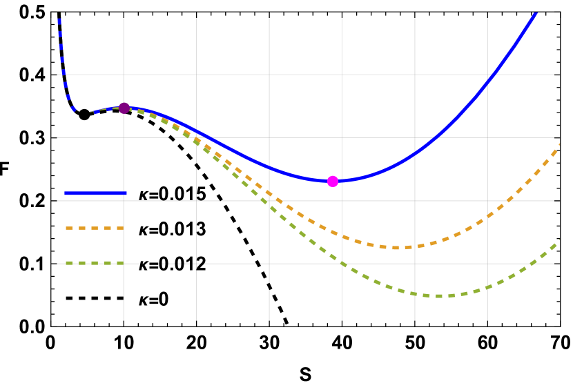
(a) F vs S plot at $J=0.2,Q=0.2$ and $l=3.2$

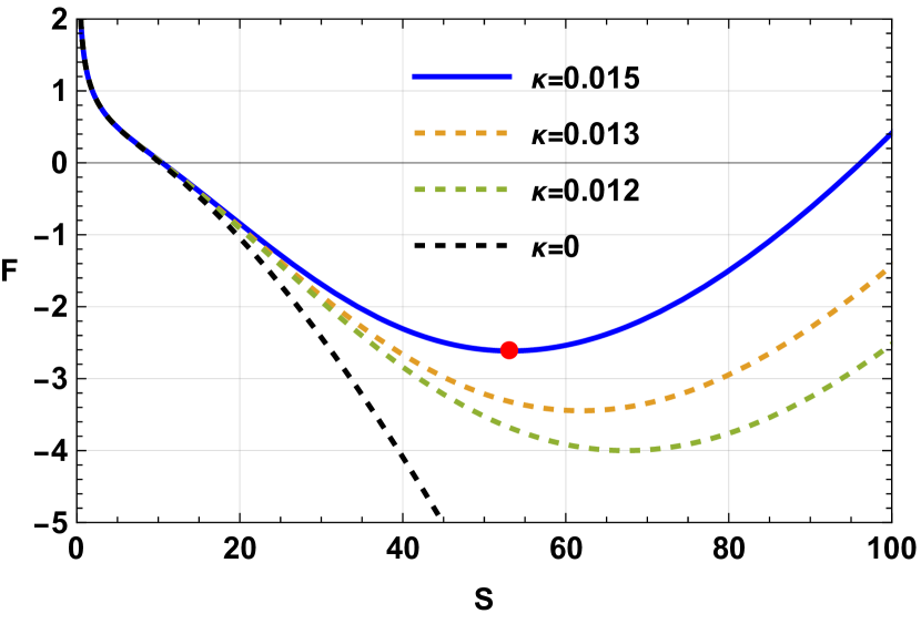
(b) F vs S plot at $J=0.5,Q=0.5$ and $l=1.5$

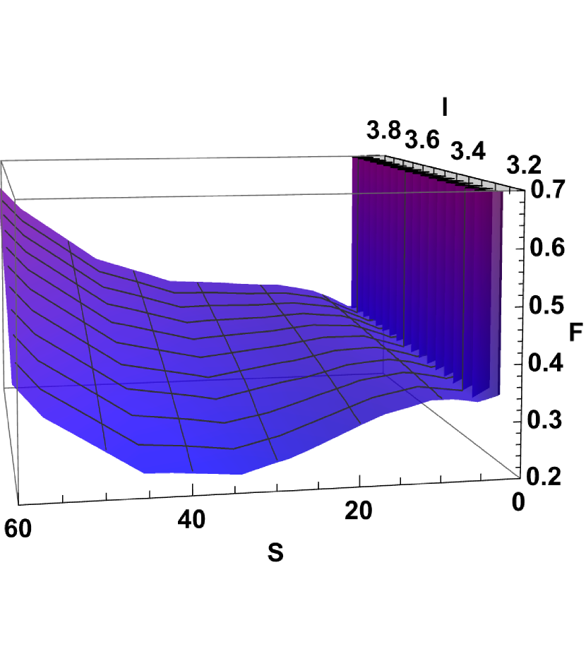
(c) 3D plot at $J=0.2,Q=0.2,\kappa=0.015$

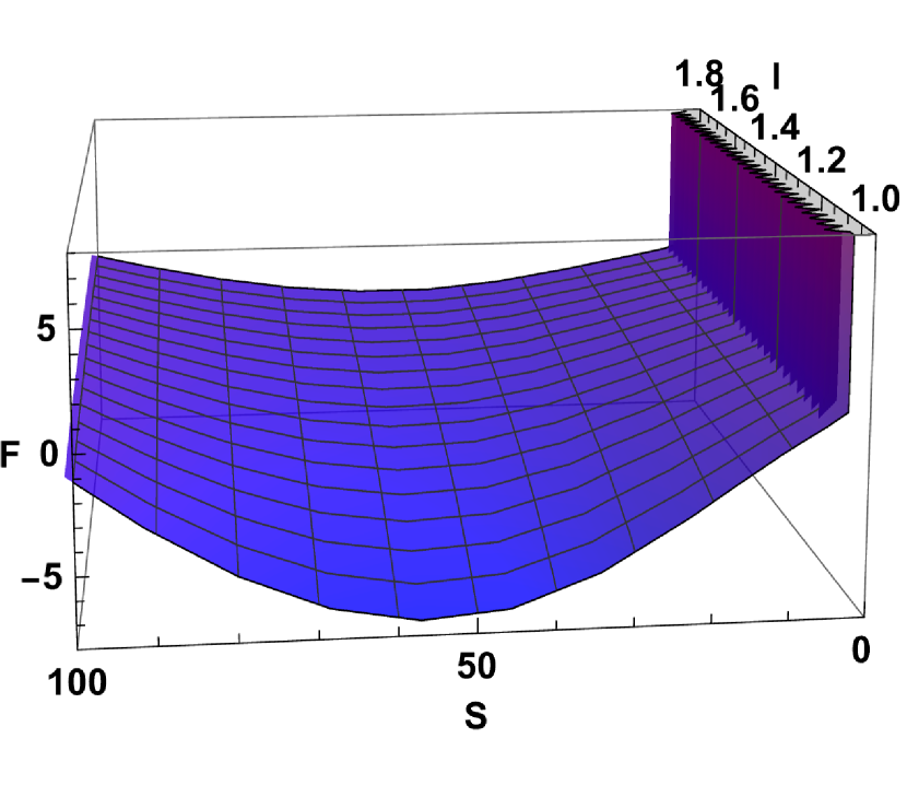
(d) 3D plot at $J=0.5,Q=0.5,\kappa=0.015$

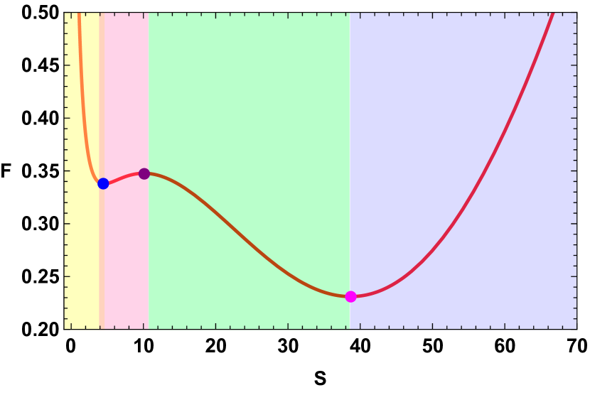
(e) BH Phases in F vs S plot($J=0.2,Q=0.2,l=3.2,\kappa=0.015$)

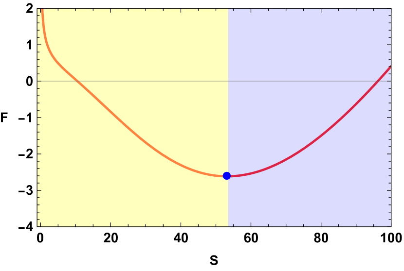
(f) BH Phases in F vs S plot($J=0.5,Q=0.5,\kappa=0.015,l=1.5$)

Figure 35: Kerr-Newman-AdS black hole: F vs S plots.

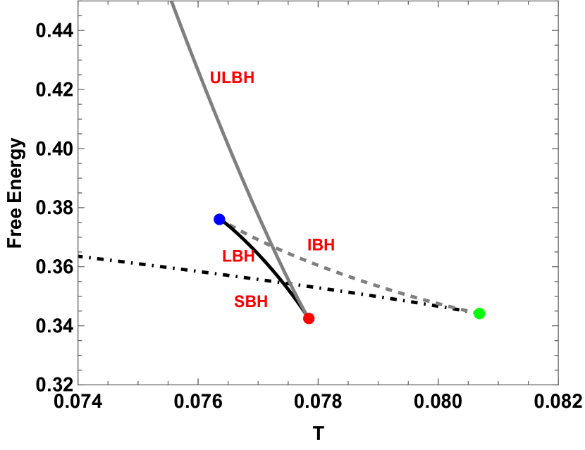
(a) F vs T plot at $J=0.2,Q=0.2,\kappa=0.015$ and $l=3.2$

(b) F vs T plot at $J=0.5,Q=0.5,\kappa=0.015$ and $l=1.5$

Figure 36: Kerr- Newman-AdS black hole: F vs T plots.

The global and local stability of black holes is shown in FIG.37, using t the free energy landscape. The off shell free energy is calculated as :

$$F_{e}=F-T_{e}S=-\frac{2\pi^{3/2}l^{2}ST\sqrt{\frac{\sinh^{-1}(\kappa S)}{\kappa}}-\sqrt{\frac{4\pi^{3}\kappa^{3}J^{2}l^{2}\left(\pi\kappa l^{2}+\sinh^{-1}(\kappa S)\right)+\left(\pi\kappa l^{2}\left(\pi\kappa Q^{2}+\sinh^{-1}(\kappa S)\right)+\sinh^{-1}(\kappa S)^{2}\right)^{2}}{\kappa^{4}}}}{2\pi^{3/2}l^{2}\sqrt{\frac{\sinh^{-1}(\kappa S)}{\kappa}}}$$ (59)

In FIG.37, the points $A,B,C_{2},E$ are both thermally and globally stable, $K^{\prime},D_{2}$ are thermally stable but only locally stable, $K,D_{3}$ are thermally and locally unstable and finally $I,J,C_{3},F$ are both globally and thermally unstable.

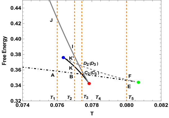
(a)

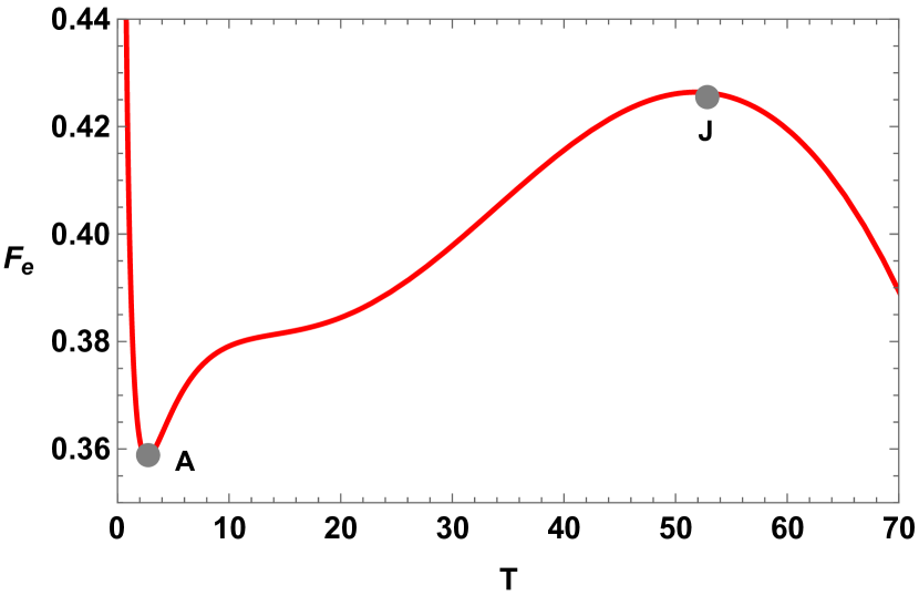
(b) $T_{e}=0.076$

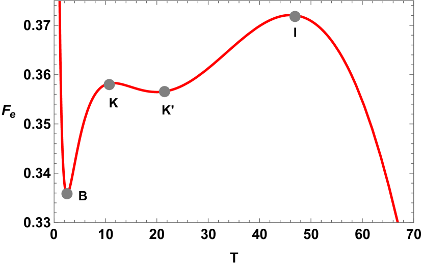
(c) $T_{e}=0.077$

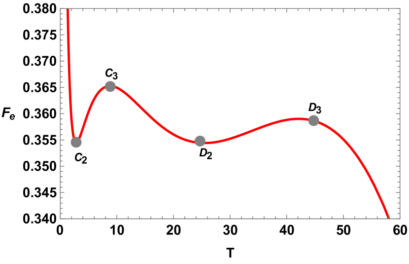
(d) $T_{e}=0.07742$

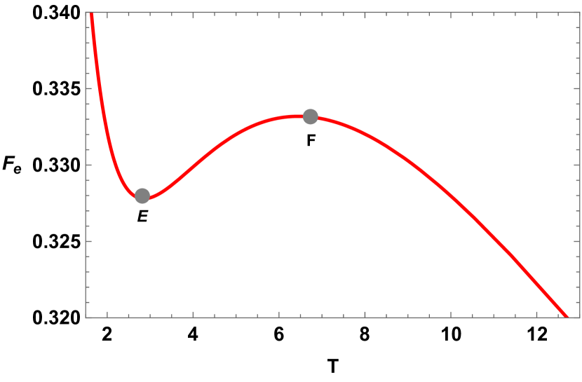
(e) $T_{e}=0.080$

(f) 3D plot for $F_{e}$ for the range $0.077<T<0.078$

Figure 37: Kerr-Newman-AdS black hole: Free energy landscape. For these plots, we have kept $J=0.2,Q=0.2,l=3.5$, and $\kappa=0.015$ fixed.

IX Thermodynamic Topology of Kerr-Newman-AdS black hole

The off-shell free energy for Kerr-Newman-AdS black hole is :

$$\mathcal{F}=M-\frac{S}{\tau}\\ =-\frac{2\pi^{3/2}l^{2}S\sqrt{\frac{\sinh^{-1}(\kappa S)}{\kappa}}-\tau\sqrt{\frac{\pi\kappa l^{2}+\sinh^{-1}(\kappa S)}{\kappa}}\sqrt{\frac{4\pi^{3}\kappa^{3}J^{2}l^{2}+2\pi^{2}\kappa^{2}l^{2}Q^{2}\sinh^{-1}(\kappa S)+\pi\kappa l^{2}\sinh^{-1}(\kappa S)^{2}+\sinh^{-1}(\kappa S)^{3}}{\kappa^{3}}}}{2\pi^{3/2}l^{2}\tau\sqrt{\frac{\sinh^{-1}(\kappa S)}{\kappa}}}$$ (60)

The components of the vector $\phi$ are

$$\phi^{S} = \frac{\alpha_{3}}{\beta_{3}}$$ (61)

$$\phi^{\Theta} = -\cot\Theta~{}\csc\Theta.$$ (62)

where

$$\alpha_{3}=-4\pi^{4}\kappa^{4}J^{2}l^{4}\tau-4\pi^{3/2}\kappa^{4}l^{2}\sqrt{\kappa^{2}S^{2}+1}\left(\frac{\sinh^{-1}(\kappa S)}{\kappa}\right)^{3/2}\\ \sqrt{\frac{4\pi^{3}\kappa^{3}J^{2}l^{2}\left(\pi\kappa l^{2}+\sinh^{-1}(\kappa S)\right)+\left(\pi\kappa l^{2}\left(\pi\kappa Q^{2}+\sinh^{-1}(\kappa S)\right)+\sinh^{-1}(\kappa S)^{2}\right)^{2}}{\kappa^{4}}}\\ -\pi^{4}\kappa^{4}l^{4}Q^{4}\tau+\pi^{2}\kappa^{2}l^{4}\tau\sinh^{-1}(\kappa S)^{2}+2\pi^{2}\kappa^{2}l^{2}Q^{2}\tau\sinh^{-1}(\kappa S)^{2}+4\pi\kappa l^{2}\tau\sinh^{-1}(\kappa S)^{3}+3\tau\sinh^{-1}(\kappa S)^{4}$$ (63)

and

$$\beta_{3}=4\pi^{3/2}\kappa^{4}l^{2}\tau\sqrt{\kappa^{2}S^{2}+1}\left(\frac{\sinh^{-1}(\kappa S)}{\kappa}\right)^{3/2}\\ \sqrt{\frac{4\pi^{3}\kappa^{3}J^{2}l^{2}\left(\pi\kappa l^{2}+\sinh^{-1}(\kappa S)\right)+\left(\pi\kappa l^{2}\left(\pi\kappa Q^{2}+\sinh^{-1}(\kappa S)\right)+\sinh^{-1}(\kappa S)^{2}\right)^{2}}{\kappa^{4}}}$$ (64)

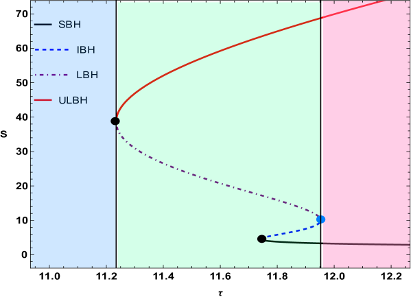
Figure 38: Kerr Newman black hole : $\tau$ vs $S$ plot. Here we have taken $J=Q=0.2$ and $l=3.2$

The expression for $\tau$ for which $\phi^{S}=0$, is calculated as:

$$\tau=\\ \frac{4\pi^{3/2}\kappa^{4}l^{2}\sqrt{\kappa^{2}S^{2}+1}\left(\frac{\sinh^{-1}(\kappa S)}{\kappa}\right)^{3/2}\sqrt{\frac{4\pi^{3}\kappa^{3}J^{2}l^{2}\left(\pi\kappa l^{2}+\sinh^{-1}(\kappa S)\right)+\left(\pi\kappa l^{2}\left(\pi\kappa Q^{2}+\sinh^{-1}(\kappa S)\right)+\sinh^{-1}(\kappa S)^{2}\right)^{2}}{\kappa^{4}}}}{-4\pi^{4}\kappa^{4}J^{2}l^{4}-\pi^{4}\kappa^{4}l^{4}Q^{4}+\pi^{2}\kappa^{2}l^{4}\sinh^{-1}(\kappa S)^{2}+2\pi^{2}\kappa^{2}l^{2}Q^{2}\sinh^{-1}(\kappa S)^{2}+4\pi\kappa l^{2}\sinh^{-1}(\kappa S)^{3}+3\sinh^{-1}(\kappa S)^{4}}$$ (65)

The KD entropy $S$ as a function of $\tau$ is presented in Fig. 38 for the parameters $J=Q=0.2$, $l=3.2$, and $\kappa=0.0015$. As expected there are four distinct branches of black holes. in the $\tau$ vs $S$ plot. In FIG .39(a)-FIG. 39(b) we provide vector plots for illustrating the components $\phi^{S}$ and $\phi^{\Theta}$ with $\tau=11.8$. We identify zero points of the vector field at $S=3.7899$, $S=5.8937$, $S=15.8937$, and $S=64.9428$.

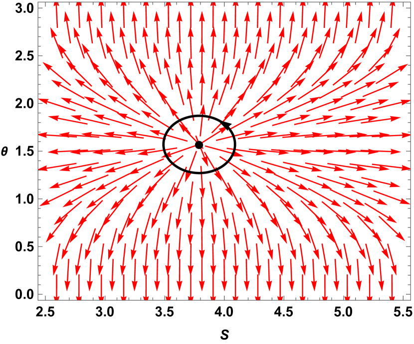
(a)

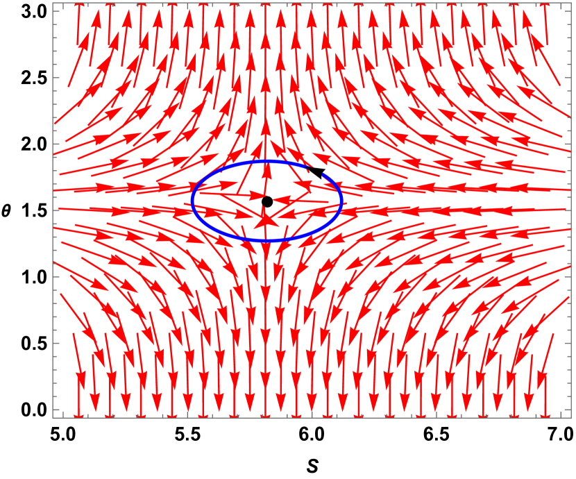
(b)

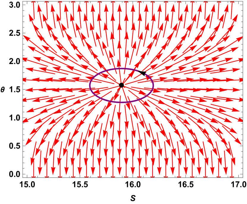
(c)

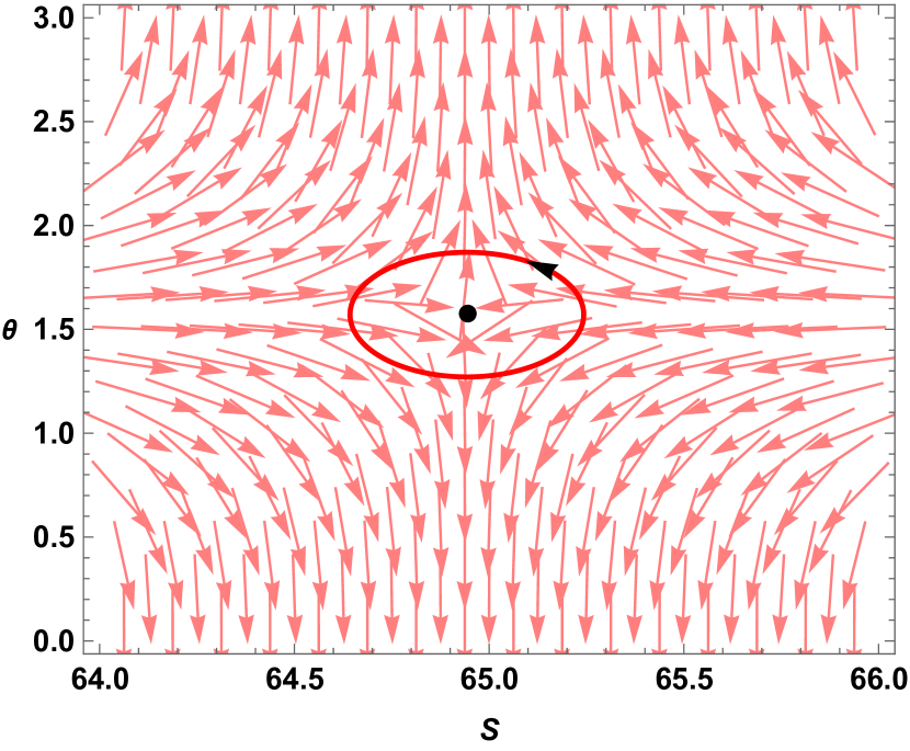
(d)

Figure 39: Kerr-Newman-AdS black holes: Vector plots of normalized ($\phi^{S}$,$\phi^{\Theta}$) field on the $S-\Theta$ plane

In FIG. 40, we presents four contour plots, each representing the computation of the winding number around these zero points. The colors in each figure correspond to the contours surrounding the zero points in the vector plots, indicating where the winding number is calculated. The winding number associated with $S=3.7899$ and $S=15.8937$ is $+1$, while that for $S=5.8186$ and $S=15.9428$ is $-1$. As the positive winding number suggests, the small and large black hole branches are stable. Conversely, the intermediate and ultra-large black hole branches are unstable as they have negative winding numbers. The total topological charge of the Kerr-Newman-AdS black hole in KD statistics is found to be $1-1+1-1=0$. Additionally, two annihilation points are observed at $(\tau_{c},S)=(11.7419,4.5450),(11.2342,38.6597)$, which is represented by black dots and one generation point is observed at $(\tau_{c},S)=(11.9527,10.0505)$ represented by a blue dot in Fig. 38.

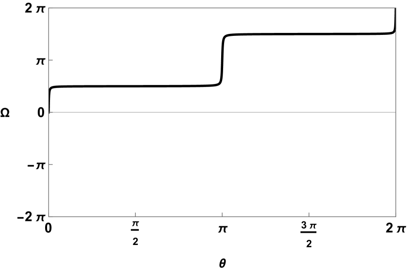
(a)

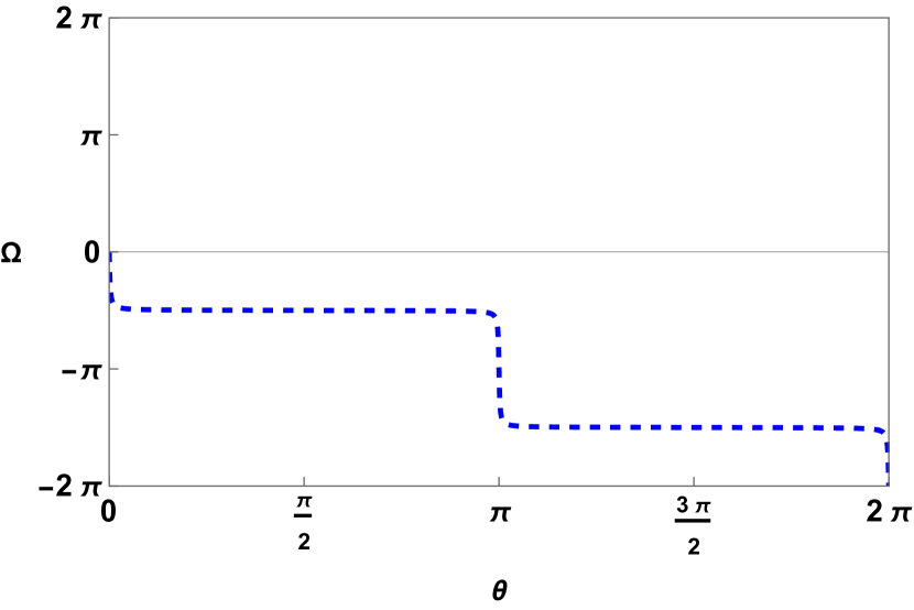
(b)

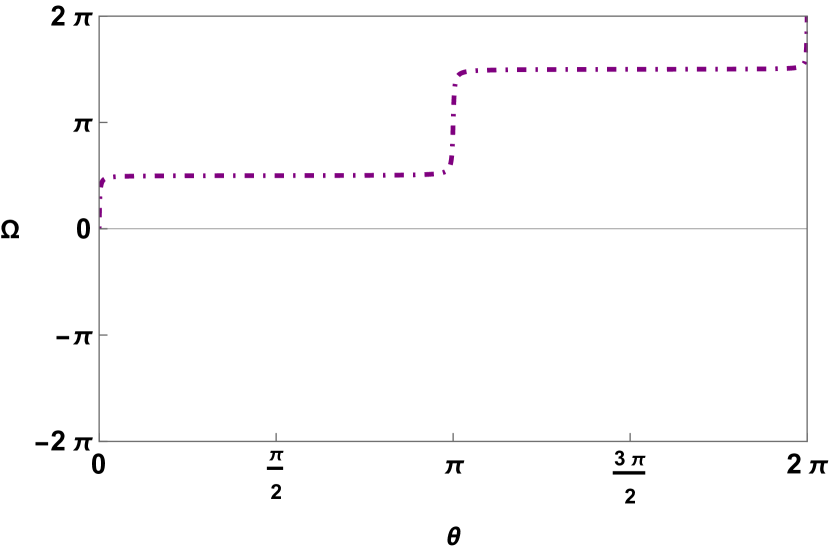
(c)

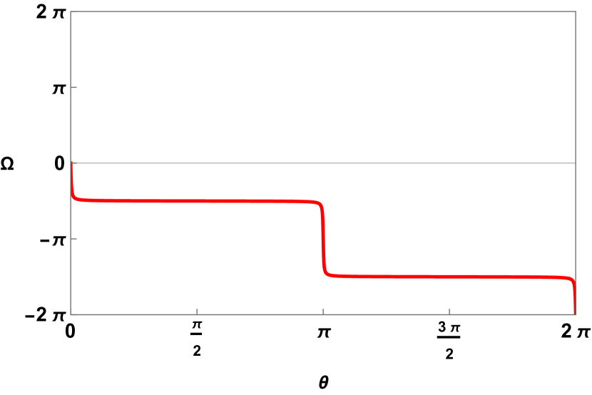
(d)

Figure 40: Kerr-Newman-AdS black holes: Winding number calculations for Kerr-Newman-AdS black holes. The black solid line in Fig.40(a) and puple dot dashed line in Fig.40(c) represents winding number for SBH and LBH respectively which equals to $+1$ and the blue solid line in Fig.40(b). Red solid line in Fig.40(d) represents winding number for IBH and ULBH respectively which euals to $-1.$

In Fig.41, we see two black hole branches: a small black hole branch(SBH) and a large black hole branch (LBH). The winding number for SBH is $+1$ which means it is stable and that for LBH is found to be $-1$ which suggests it is an unstable branch. Moreover we found a annihilation point in $(\tau=2.9231,S=53.2136)$ represented by the black dot in the Fig.41(a)

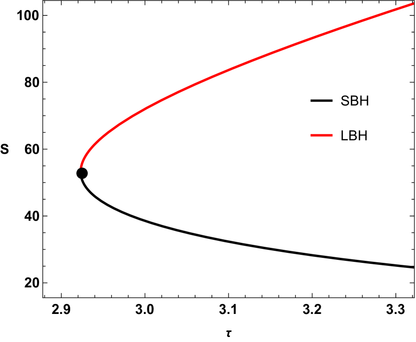
(a)

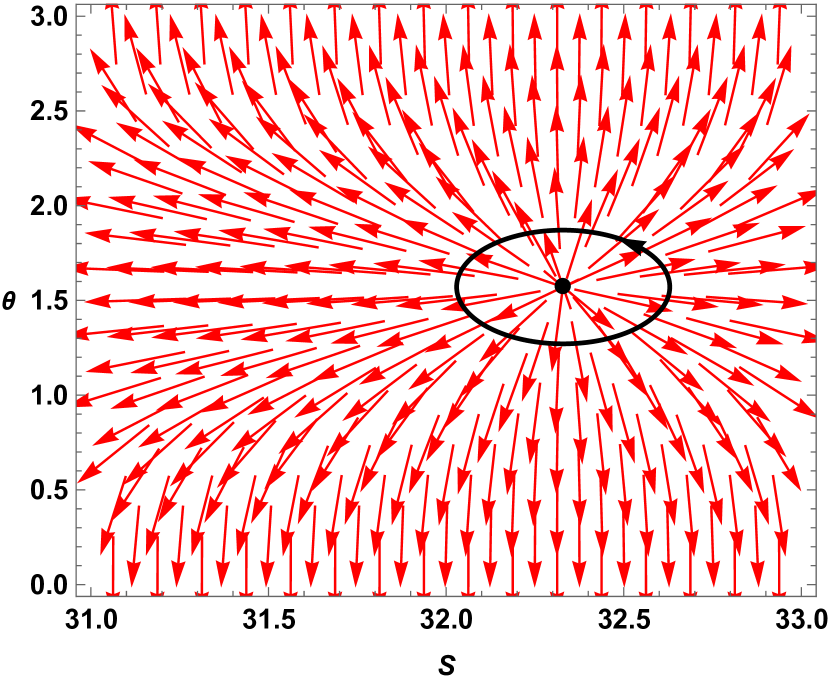
(b)

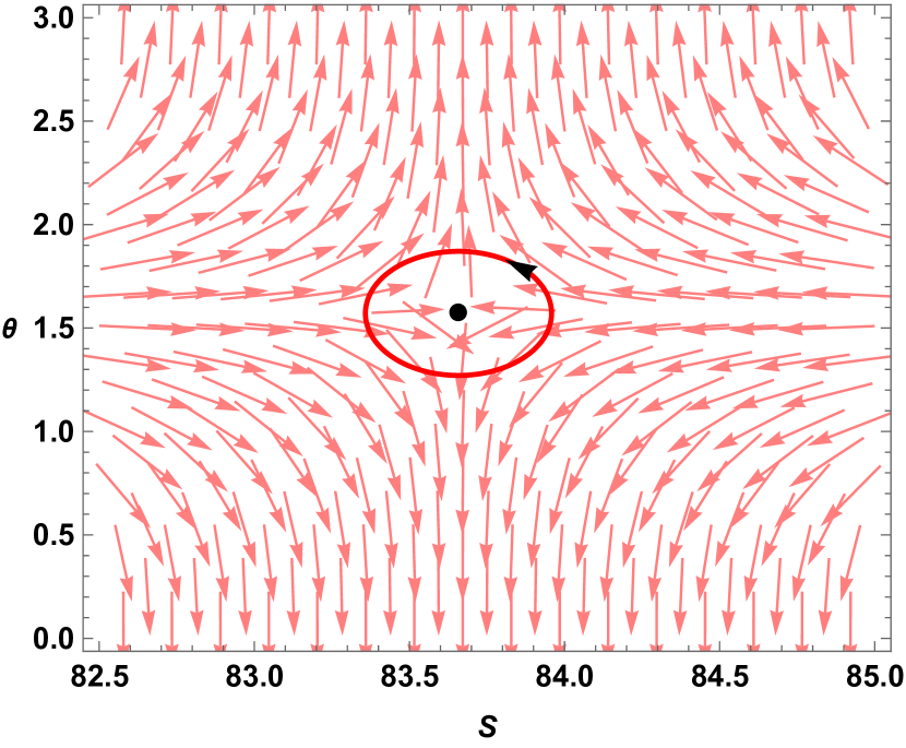
(c)

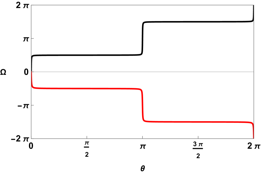
(d)

Figure 41: Kerr-Newman-AdS black holes: In Fig.41(a), $\tau$ vs $S$ is plotted for Kerr-Newman-AdS black holes when $J=Q=0.5,l=1.5$ and $\kappa=0.015$ is taken. In Fig.41(b) and Fig.41(c) vectorplots are shown in $S-\theta$ plane where the zero point (S,$\theta$)= $(32.3295,\pi/2)$ in Fig.41(b) is on the SBH and the zero point (S,$\theta$)= $(83.6580,\pi/2)$ in Fig.41(c) is on the LBH. The winding number calculation is shown in Fig.41(d) where the black solid line in Fig.41(d) represents winding number for SBH which equals to $+1$ and the red solid line in Fig.41(d) represents winding number for LBH which euals to $-1.$

The number of branches in the $\tau$ vs $S$ graph changes with a change in the value of $J,Q$ and $l.$ We observe either four or two branches depending on the values of thermodynamic parameters. However, the topological charge remains invariant when the values of $J,Q,l$ and $\kappa$ are varied. In Fig. 42(a) and Fig. 42(b), we show the variation of $\kappa$ with $J=Q=0.2$, $l=3.2$, and with $J=Q=0.5$, $l=1.5$, respectively. Fig. 42(c) illustrates the variation of $J$ with $Q=0.2$, $l=3.2$, and $\kappa=0.015$ held constant. Fig. 42(d) demonstrates the variation of $Q$ while keeping $J=0.2$, $l=3.2$, and $\kappa=0.015$ fixed. Additionally, in Fig. 42(e), we depict the variation of $l$ with $Q=J=0.2$ and $\kappa=0.015$ fixed.

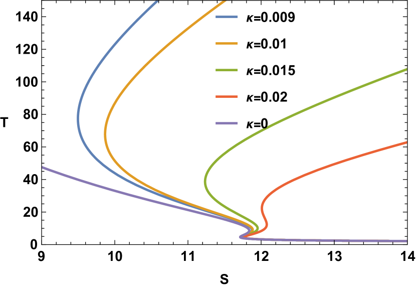
(a)

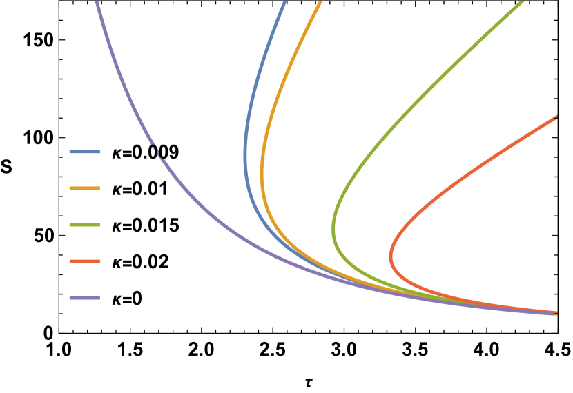
(b)

(c)

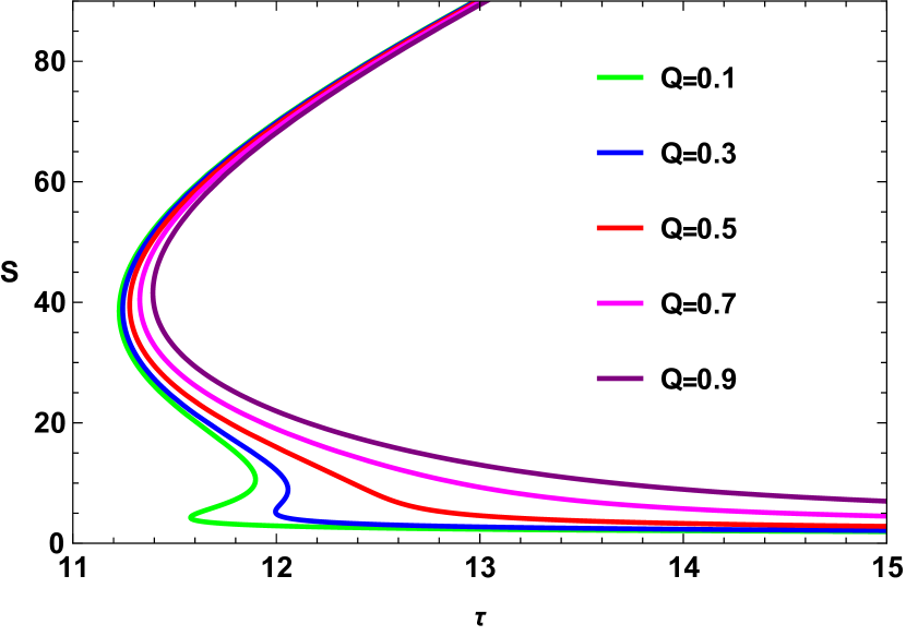
(d)

(e)

Figure 42: Variations of $\tau$ vs $S$ plots for kerr-sen-ads black holes with different thermodynamic parameters

In conclusion, for the Kerr-Newman-AdS black hole in KD statistics, the topological charge is $0$ and it is observed that, the topological charge is independent of other thermodynamic parameters.

X Thermodynamic geometry of Kerr-Newman-AdS black holes

The line element for the Ruppeiner metric in the Kerr-Newman-AdS black hole could be written as :

$$dS_{R}^{2}=\frac{1}{T}\left(\frac{\partial^{2}M}{\partial S^{2}}dS^{2}+\frac{\partial^{2}M}{\partial J^{2}}dJ^{2}+\frac{\partial^{2}M}{\partial Q^{2}}dQ^{2}+2\frac{\partial^{2}M}{\partial S\partial J}dSdJ+2\frac{\partial^{2}M}{\partial J\partial Q}dJdQ+2\frac{\partial^{2}M}{\partial S\partial Q}dSdQ\right)$$

and the line element for the GTD metric in the Kerr-Newman-AdS black hole is given by:

$$dS_{G}^{2}=S\left(\frac{\partial M}{\partial S}\right)\left(-\frac{\partial^{2}M}{\partial S^{2}}dS^{2}+\frac{\partial^{2}M}{\partial J^{2}}dJ^{2}+\frac{\partial^{2}M}{\partial Q^{2}}dQ^{2}\right)$$

We see from Fig.43(b) that the Ruppeiner scalar is plotted against the Kaniadakis entropy for $J=Q=0.2$ and $L=3.2$. We see the Ruppeiner scalar curve has three singularities at $S=1.174,12.392$ and $38.407$ for $\kappa=0.015$ whereas in Fig.44(b) we see that for $J=Q=0.5$ and $L=1.5$ there is only one singularity at $S=53.090$ for $\kappa=0.015$. The GTD scalar on the other hand has singularities at $S=4.545,10.051$ and $38.659$ for $J=Q=0.2$ and $L=3.2$ as can be seen in Fig.45(b). We see from Fig.46(b) that for $J=Q=0.5$ and $L=1.5$ there is only one singularity at $S=53.214$. The singularities in the GTD scalar curves agree with the points of Davies type phase transitions obtained from the heat capacity curves.

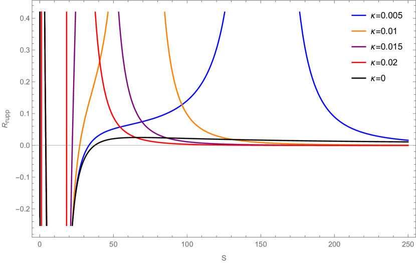
(a) For all $\kappa$

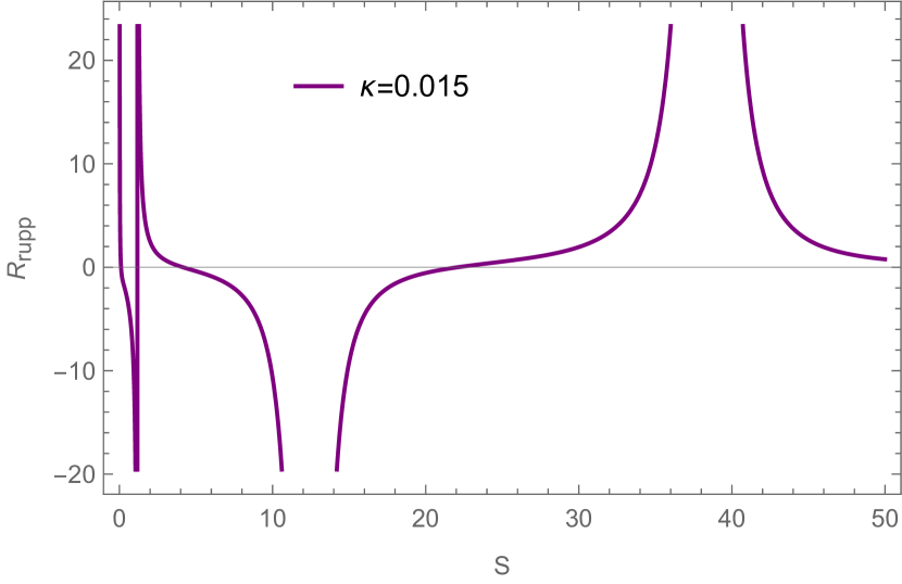
(b) For $\kappa=0.015$

Figure 43: The Ruppeiner scalar versus Entropy plot for Kerr-Newman-AdS black hole for $J=Q=0.2$ and $L=3.2$.

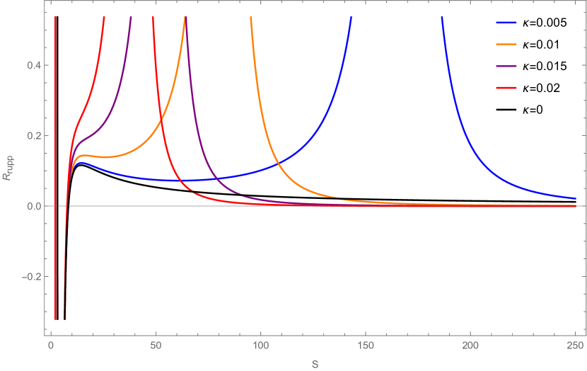
(a) For all $\kappa$

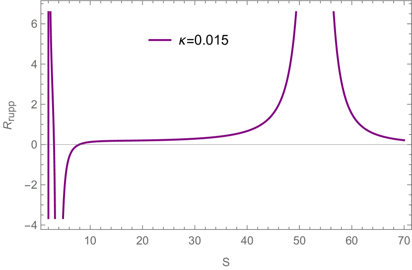
(b) For $\kappa=0.015$

Figure 44: The Ruppeiner scalar versus Entropy plot for Kerr-Newman-AdS black hole for $J=Q=0.5$ and $L=1.5$.

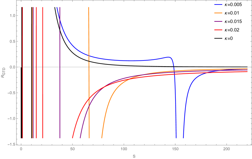
(a) For all $\kappa$

(b) For $\kappa=0.015$

Figure 45: The GTD scalar versus Entropy plot for Kerr-Newman-AdS black hole for $J=Q=0.2$ and $L=3.2$.

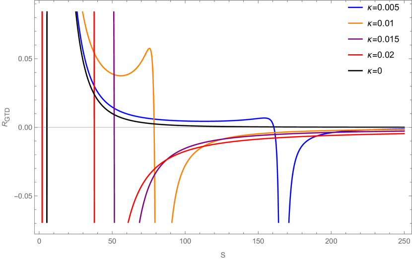
(a) For all $\kappa$

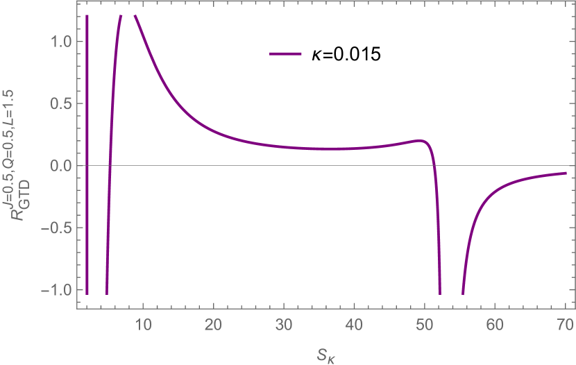
(b) For $\kappa=0.015$

Figure 46: The GTD scalar versus Entropy plot for Kerr-Newman-AdS black hole for $J=Q=0.5$ and $L=1.5$.

XI Conclusions

In this paper, we studied the thermodynamic properties and phase transitions in rotating anti-de Sitter (AdS) black holes by applying the Kaniadakis entropy framework. We analyzed three rotating AdS black hole systems: the Kerr-AdS-black hole, the Kerr-Sen-AdS black hole, and the Kerr-Newman-AdS black hole. We assessed their thermodynamic quantities, phase transitions, thermodynamic topology and thermodynamic geometry within the Kaniadakis statistical framework.

We first evaluated the thermodynamic quantities of each black hole using Kaniadakis entropy. For all three black holes, the impact of the Kaniadakis parameter $\kappa$ on the black hole mass and temperature becomes more pronounced at higher values of Kaniadakis entropy $S$. The range of $S$ within which the black hole mass in Kaniadakis statistics approximates the mass in Gibbs-Boltzmann statistics varies with $\kappa$. In the $T$ vs. $S$ diagram, Gibbs-Boltzmann statistics typically show either one or three branches: one branch indicates no phase transition, while three branches correspond to a Van der Waals-like small-intermediate-large black hole phase transition. In contrast, when using Kaniadakis entropy, we observe either two or four branches. Besides the small-intermediate-large black hole branches, an additional branch, the ultra-large black hole branch (ULBH), emerges. The number of branches in the $T$ vs. $S$ diagram depended on the thermodynamic parameters of the black hole system.

Next, we examined the heat capacity of all three black hole systems. In Gibbs-Boltzmann statistics, the number of discontinuities in the heat capacity versus entropy is either zero or two. Conversely, in Kaniadakis statistics, the number of discontinuities is either one or three. The sign of the heat capacity indicates the stability of the system. In Kaniadakis statistics, we find either two stable and two unstable branches or one stable and one unstable branch. In Gibbs-Boltzmann statistics, we found either two stable and one unstable branch or just one stable branch.

We also studied the free energy $F$ as a function of $S$ and $T$ for each black hole system. Moreover, we used the free energy landscape to estimate the stability of the black hole solutions. By constructing an off-shell free energy with an ensemble temperature $T_{e}$, we determined that a physical black hole can only exist at the extremal points of the off-shell free energy. Thus, at the maximum point of the off-shell free energy curve, a black hole is considered unstable, whereas at the minimum point, the black hole is considered stable. This approach allows us to analyze both the global and local stability of each black hole.

Next,we investigated the thermodynamic topology of each black hole system. In our analysis, using the off shell free energy method, all the black holes are treated as topological defects.The winding numbers at those defects is calculated in order to understand the topology of the thermodynamic spaces of these black holes.Our primary motivation was to explore the impact of KD entropy on the topological charge of the black hole.Our analysis revealed that, under KD statistics, the topological charge for all three black hole systems is $0$, whereas in Gibbs-Boltzmann (GB) statistics, the charge is $+1$. Furthermore, in KD statistics, we observed one generation point and one annihilation point, while in GB statistics, we found one annihilation point and one generation point. This indicates that transitioning from GB to KD statistics results in change of the topological charge and the topological class of these rotating black holes.The topological charge is found to be independent of all the thermodynamic parameter in both the statistics.

This paper also explored the thermodynamic geometry of these rotating AdS black holes by applying the Ruppeiner and geometrothermodynamic (GTD) formalisms. Our analysis revealed that singularities in the scalar curvature are present in both statistical frameworks. Notably, in the Ruppeiner formalism, these singularities do not align with the Davies points observed in the heat capacity curves previously analyzed. Conversely, in the GTD formalism, the singularities in the scalar curvature matches exactly with the Davies points found in the heat capacity curves.

Hence the impact of KD entropy on thermodynamic phase space of rotating Ads black hole is found to be very crucial.This is confirmed by the study of thermodynamic topology and thermodynamic geometry in this paper.It would be interesting to see how KD entropy and other non extensive entropy correction impact the thermodynamics of different black hole systems in different ensembles,other than the canonical ensemble. We plan to address this in our future works.

XII Acknowledgments

BH would like to thank DST-INSPIRE, Ministry of Science and Technology fellowship program, Govt. of India for awarding the DST/INSPIRE Fellowship[IF220255] for financial support.

References

- [1] J. D. Bekenstein, Black holes and entropy, Phys. Rev. D 7, 2333-2346 (1973) doi:10.1103/PhysRevD.7.2333
- [2] S. W. Hawking, Black hole explosions, Nature 248, 30-31 (1974) doi:10.1038/248030a0
- [3] S. W. Hawking, Particle Creation by Black Holes, Commun. Math. Phys. 43, 199-220 (1975) [erratum: Commun. Math. Phys. 46, 206 (1976)] doi:10.1007/BF02345020
- [4] J. M. Bardeen, B. Carter and S. W. Hawking, The Four laws of black hole mechanics, Commun. Math. Phys. 31, 161-170 (1973) doi:10.1007/BF01645742
- [5] R. M. Wald, Entropy and black-hole thermodynamics, Phys. Rev. D 20, 1271-1282 (1979) doi:10.1103/PhysRevD.20.1271
- [6] Jacob D Bekenstein. Black-hole thermodynamics, Physics Today, 33(1):24–31, 1980.
- [7] R. M. Wald, The thermodynamics of black holes, Living Rev. Rel. 4, 6 (2001) doi:10.12942/lrr-2001-6 [arXiv:gr-qc/9912119 [gr-qc]].
- [8] S.Carlip, Black Hole Thermodynamics, Int. J. Mod. Phys. D 23, 1430023 (2014) doi:10.1142/S0218271814300237 [arXiv:1410.1486 [gr-qc]].
- [9] A.C.Wall, A Survey of Black Hole Thermodynamics, [arXiv:1804.10610 [gr-qc]].
- [10] P.Candelas and D.W.Sciama, Irreversible Thermodynamics of Black Holes, Phys. Rev. Lett. 38, 1372-1375 (1977) doi:10.1103/PhysRevLett.38.1372
- [11] S. Mahapatra, P. Phukon and T. Sarkar, Phys. Rev. D 84, 044041 (2011) doi:10.1103/PhysRevD.84.044041 [arXiv:1103.5885 [hep-th]].
- [12] P. C. W. Davies, Thermodynamic Phase Transitions of Kerr-Newman Black Holes in De Sitter Space, Class. Quant. Grav. 6, 1909 (1989) doi:10.1088/0264-9381/6/12/018
- [13] S. W. Hawking and D. N. Page, Thermodynamics of Black Holes in anti-De Sitter Space, Commun. Math. Phys. 87, 577 (1983) doi:10.1007/BF01208266
- [14] A. Curir, Rotating black holes as dissipative spin-thermodynamical systems, General Relativity and Gravitation, 13, 417, (1981) doi:10.1007/BF00756588
- [15] Anna Curir, Black hole emissions and phase transitions, General Relativity and Gravitation, 13, 1177, (1981) doi:10.1007/BF00759866
- [16] D. Pavon and J. M. Rubi, Nonequilibrium Thermodynamic Fluctuations of Black Holes, Phys. Rev. D 37, 2052-2058 (1988) doi:10.1103/PhysRevD.37.2052
- [17] D. Pavon, Phase transition in Reissner-Nordstrom black holes, Phys. Rev. D 43, 2495-2497 (1991) doi:10.1103/PhysRevD.43.2495
- [18] O. Kaburaki, Critical behavior of extremal Kerr-Newman black holes, Gen. Rel. Grav. 28, 843 (1996)
- [19] R. G. Cai, Z. J. Lu and Y. Z. Zhang, Critical behavior in (2+1)-dimensional black holes, Phys. Rev. D 55, 853-860 (1997) doi:10.1103/PhysRevD.55.853 [arXiv:gr-qc/9702032 [gr-qc]].
- [20] R. G. Cai and J. H. Cho, Thermodynamic curvature of the BTZ black hole, Phys. Rev. D 60, 067502 (1999) doi:10.1103/PhysRevD.60.067502 [arXiv:hep-th/9803261 [hep-th]].
- [21] Y. H. Wei, Thermodynamic critical and geometrical properties of charged BTZ black hole, Phys. Rev. D 80, 024029 (2009) doi:10.1103/PhysRevD.80.024029
- [22] K. Bhattacharya, S. Dey, B. R. Majhi and S. Samanta, General framework to study the extremal phase transition of black holes, Phys. Rev. D 99, no.12, 124047 (2019) doi:10.1103/PhysRevD.99.124047 [arXiv:1903.03434 [gr-qc]].
- [23] D. Kastor, S. Ray and J. Traschen, Enthalpy and the Mechanics of AdS Black Holes, Class. Quant. Grav. 26, 195011 (2009) doi:10.1088/0264-9381/26/19/195011 [arXiv:0904.2765 [hep-th]].
- [24] B. P. Dolan, The cosmological constant and the black hole equation of state, Class. Quant. Grav. 28, 125020 (2011) doi:10.1088/0264-9381/28/12/125020 [arXiv:1008.5023 [gr-qc]].
- [25] B. P. Dolan, Pressure and volume in the first law of black hole thermodynamics, Class. Quant. Grav. 28, 235017 (2011) doi:10.1088/0264-9381/28/23/235017 [arXiv:1106.6260 [gr-qc]].
- [26] B. P. Dolan, Compressibility of rotating black holes, Phys. Rev. D 84, 127503 (2011) doi:10.1103/PhysRevD.84.127503 [arXiv:1109.0198 [gr-qc]].
- [27] B. P. Dolan, Where Is the PdV in the First Law of Black Hole Thermodynamics?, doi:10.5772/52455 [arXiv:1209.1272 [gr-qc]].
- [28] D. Kubiznak and R. B. Mann, P-V criticality of charged AdS black holes, JHEP 07, 033 (2012) doi:10.1007/JHEP07(2012)033 [arXiv:1205.0559 [hep-th]].
- [29] D. Kubiznak, R. B. Mann and M. Teo, Black hole chemistry: thermodynamics with Lambda, Class. Quant. Grav. 34, no.6, 063001 (2017) doi:10.1088/1361-6382/aa5c69 [arXiv:1608.06147 [hep-th]].
- [30] K. Bhattacharya, B. R. Majhi and S. Samanta, Van der Waals criticality in AdS black holes: a phenomenological study, Phys. Rev. D 96, no.8, 084037 (2017) doi:10.1103/PhysRevD.96.084037 [arXiv:1709.02650 [gr-qc]].
- [31] David Kubizˇn´ak and Robert B. Mann. P-v criticality of charged AdS black holes. Journal of High Energy Physics, 2012(7),2012.
- [32] Natacha Altamirano, David Kubizˇn ´ak, and Robert B. Mann. Reentrant phase transitions in rotating anti–de sitter black holes. Physical Review D, 88(10),2013.
- [33] Natacha Altamirano, David Kubizˇn´ak, Robert B Mann, and Zeinab Sherkatghanad. Kerr-ads analogue of triple point and solid/liquid/gas phase transition. Classical and Quantum Gravity, 31(4):042001, 2014.
- [34] Shao-Wen Wei and Yu-Xiao Liu. Triple points and phase diagrams in the extended phase space of charged gauss-bonnet black holes in ads space., Phys. Rev. D, 90:044057,2014.
- [35] Antonia M. Frassino, David Kubiznak, Robert B. Mann, and Fil Simovic, ,Multiple reentrant phase transitions and triple points in lovelock thermodynamics., Journal of High Energy Physics, 2014(9),2014.
- [36] Rong-Gen Cai, Li-Ming Cao, Li Li, and Run-Qiu Yang. P-v criticality in the extended phase space of gauss-bonnet black holes in AdS space. Journal of High Energy Physics, 2013(9), 2013
- [37] Hao Xu, Wei Xu, and Liu Zhao. Extended phase space thermodynamics for third-order lovelock black holes in diverse dimensions., The European Physical Journal C, 74(9),2014.
- [38] Brian P Dolan, Anna Kostouki, David Kubizˇn´ak, and Robert B Mann. Isolated critical point from lovelock gravity. Classical and Quantum Gravity, 31(24):242001, 2014
- [39] Robie A. Hennigar, W. G. Brenna, and Robert B. Mann. P-v criticality in quasitopological gravity., Journal of High Energy Physics, 2015(7), 2015.
- [40] Robie Hennigar and Robert Mann. Reentrant phase transitions and van der waals behaviour for hairy black holes. Entropy17(12):8056–8072, 2015.
- [41] Robie A. Hennigar, Robert B. Mann, and Erickson Tjoa. Superfluid black holes. Physical Review Letters 118(2),2017.
- [42] De-Cheng Zou,Ruihong Yue, and Ming Zhang. Reentrant phase transitions of higher-dimensional ads black holes in drgt massive gravity. The European Physical Journal C, 77(4),2017.
- [43] Gogoi, Naba Jyoti and Phukon, Prabwal. Thermodynamic geometry of 5D -charged black holes in extended thermodynamic space. Phys. Rev. D, 103(126008),2021. doi:10.1103/PhysRevD.103.126008.
- [44] J. Sadeghi, M. Shokri, S. Gashti Noori and M. R. Alipour, RPS thermodynamics of Taub–NUT AdS black holes in the presence of central charge and the weak gravity conjecture. Gen. Rel. Grav. 54 (2022)
- [45] Y. Ladghami, B. Asfour, A. Bouali, A. Errahmani and T. Ouali, 4D-EGB black holes in RPS thermodynamics, Phys. Dark Univ. 41 (2023),
- [46] X. Kong, Z. Zhang and L. Zhao, Restricted phase space thermodynamics of charged AdS black holes in conformal gravity, Chin. Phys. C 47 (2023)
- [47] M. R. Alipour, J. Sadeghi and M. Shokri, WGC and WCCC of black holes with quintessence and cloud strings in RPS space, Nucl. Phys. B 990 (2023)
- [48] T. Wang and L. Zhao, Black hole thermodynamics is extensive with variable Newton constant, Phys. Lett. B 827 (2022)
- [49] G. Zeyuan and L. Zhao, Restricted phase space thermodynamics for AdS black holes via holography, Class. Quant. Grav. 39 (2022)
- [50] Z. Gao, X. Kong and L. Zhao, Thermodynamics of Kerr-AdS black holes in the restricted phase space, Eur. Phys. J. C 82 (2022)
- [51] S. Dutta and G. S. Punia, String theory corrections to holographic black hole chemistry, Phys. Rev. D 106, no.2, 026003 (2022)
- [52] T. F. Gong, J. Jiang and M. Zhang, Holographic thermodynamics of rotating black holes, JHEP 06, 105 (2023)
- [53] W. Cong, D. Kubiznak, R. B. Mann and M. R. Visser, Holographic CFT phase transitions and criticality for charged AdS black holes, JHEP 08, 174 (2022)
- [54] M. R. Visser, Holographic thermodynamics requires a chemical potential for color, Phys. Rev. D 105, no.10, 106014 (2022)
- [55] C. Tsallis and L. J. L. Cirto, Eur. Phys. J. C 73, 2487 (2013).
- [56] H. Quevedo, M. N. Quevedo and A. Sanchez, Eur. Phys. J. C 79, 229 (2019).
- [57] C. Tsallis, J. Statist. Phys. 52, 479 (1988).
- [58] J. D. Barrow, Phys. Lett. B 808, 135643 (2020).
- [59] S. Nojiri, S. D. Odintsov and V. Faraoni, Phys. Rev. D 105, 044042 (2022).
- [60] A. Rényi, Acta Math. Acad. Sci. Hung. 10, 193 (1959).
- [61] B. D. Sharma and D. P. Mittal, J. Comb. Inf. Syst. Sci. 2, 122 (1977).
- [62] G. Kaniadakis, Physica A 296, 405 (2001).
- [63] G. Kaniadakis, Phys. Rev. E 66, 056125 (2002).
- [64] G. Kaniadakis, Phys. Rev. E 72, 036108 (2005).
- [65] G. Kaniadakis, M. Lissia and A. M. Scarfone, Phys. Rev. E 71, 046128 (2005).
- [66] G. Kaniadakis, P. Quarati and A. M. Scarfone, Physica 305, 76 (2002).
- [67] G. G. Luciano, Entropy 24, 1712 (2022).
- [68] H. Moradpour, A.H. Ziaie, M. Kord Zangeneh, Eur. Phys. J. C 80, 732 (2020).
- [69] A. Lymperis, S. Basilakos and E. N. Saridakis, Eur. Phys. J. C 81, 1037 (2021).
- [70] N. Drepanou, A. Lymperis, E. N. Saridakis and K. Yesmakhanova, Eur. Phys. J. C 82, 449 (2022).
- [71] A. Sheykhi, [arXiv:2302.13012 [gr-qc]].
- [72] Giuseppe Gaetano Luciano and Emmanuel Saridakis,2023,arXiv.2308.12669,gr-qc,
- [73] A. Hernández-Almada, G. Leon, J. Magaña, M. A. García-Aspeitia, V. Motta, E. N. Saridakis and K. Yesmakhanova, Mon. Not. Roy. Astron. Soc. 511, 4147 (2022).
- [74] A. Hernández-Almada, G. Leon, J. Magaña, M. A. García-Aspeitia, V. Motta, E. N. Saridakis, K. Yesmakhanova and A. D. Millano, Mon. Not. Roy. Astron. Soc. 512, 5122 (2022).
- [75] G. Lambiase, G. G. Luciano and A. Sheykhi, [arXiv:2307.04027 [gr-qc]].
- [76] I. Cimidiker, M. P. Dabrowski and H. Gohar, Class. Quant. Grav. 40, 145001 (2023).
- [77] A. Kempf, G. Mangano and R. B. Mann, Phys. Rev. D 52, 1108 (1995).
- [78] L. Buoninfante, G. G. Luciano, L. Petruzziello and F. Scardigli, Phys. Lett. B 824, 136818 (2022).
- [79] Jafar Sadeghi and Mohammad Ali S. Afshar and Mohammad Reza Alipour and Saeed Noori Gashti,2024,arXiv 2407.20779gr-qc
- [80] Kumar.N,Relativistic correction to black hole entropy. Gen Relativ Gravit 56, 47 (2024).
- [81] H. Quevedo and A. Sanchez, Geometric description of BTZ black holes thermodynamics, Phys. Rev. D 79, 024012 (2009) doi:10.1103/PhysRevD.79.024012 [arXiv:0811.2524 [gr-qc]].
- [82] M. Akbar, H. Quevedo, K. Saifullah, A. Sanchez and S. Taj, Thermodynamic Geometry Of Charged Rotating BTZ Black Holes, Phys. Rev. D 83, 084031 (2011) doi:10.1103/PhysRevD.83.084031 [arXiv:1101.2722 [gr-qc]].
- [83] S. H. Hendi and R. Naderi, Geometrothermodynamics of black holes in Lovelock gravity with a nonlinear electrodynamics, Phys. Rev. D 91, no.2, 024007 (2015) doi:10.1103/PhysRevD.91.024007 [arXiv:1510.06269 [hep-th]].
- [84] T. Sarkar, G. Sengupta and B. Nath Tiwari, On the thermodynamic geometry of BTZ black holes, JHEP 11, 015 (2006) doi:10.1088/1126-6708/2006/11/015 [arXiv:hep-th/0606084 [hep-th]].
- [85] S. H. Hendi, A. Sheykhi, S. Panahiyan and B. Eslam Panah, Phase transition and thermodynamic geometry of Einstein-Maxwell-dilaton black holes, Phys. Rev. D 92, no.6, 064028 (2015) doi:10.1103/PhysRevD.92.064028 [arXiv:1509.08593 [hep-th]].
- [86] R. Banerjee, B. R. Majhi and S. Samanta, Thermogeometric phase transition in a unified framework, Phys. Lett. B 767, 25-28 (2017) doi:10.1016/j.physletb.2017.01.040 [arXiv:1611.06701 [gr-qc]].
- [87] K. Bhattacharya and B. R. Majhi, Thermogeometric description of the van der Waals like phase transition in AdS black holes, Phys. Rev. D 95, no.10, 104024 (2017) doi:10.1103/PhysRevD.95.104024 [arXiv:1702.07174 [gr-qc]].
- [88] K. Bhattacharya and B. R. Majhi, Thermogeometric study of van der Waals like phase transition in black holes: an alternative approach, Phys. Lett. B 802, 135224 (2020) doi:10.1016/j.physletb.2020.135224 [arXiv:1903.10370 [gr-qc]].
- [89] N. J. Gogoi, G. K. Mahanta and P. Phukon, Geodesics in geometrothermodynamics (GTD) type II geometry of 4D asymptotically anti-de-Sitter black holes, Eur. Phys. J. Plus 138, no.4, 345 (2023) doi:10.1140/epjp/s13360-023-03938-x
- [90] P. Kumar, S. Mahapatra, P. Phukon and T. Sarkar, Geodesics in Information Geometry : Classical and Quantum Phase Transitions, Phys. Rev. E 86, 051117 (2012) doi:10.1103/PhysRevE.86.051117 [arXiv:1210.7135 [cond-mat.stat-mech]].
- [91] P.V.P. Cunha, E. Berti, and C.A.R. Herdeiro, Light Ring Stability in Ultra-Compact Objects, Phys. Rev. Lett. 119, 251102 (2017).
- [92] P.V.P. Cunha, and C.A.R. Herdeiro, Stationary Black Holes and Light Rings, Phys. Rev. Lett. 124, 181101 (2020).
- [93] S.-W. Wei, Topological charge and black hole photon spheres, Phys. Rev. D 102, 064039 (2020).
- [94] M. Guo and S. Gao, Universal properties of light rings for stationary axisymmetric spacetimes, Phys. Rev. D 103, 104031 (2021).
- [95] M. Guo, Z. Zhong, J. Wang, and S. Gao, Light rings and long-lived modes in quasiblack hole spacetimes, Phys. Rev. D 105, 024049 (2022).
- [96] S.-P. Wu and S.-W. Wei, Topology of light rings for extremal and nonextremal Kerr-Newman-Taub-NUT black holes without Z2 symmetry, Phys. Rev. D 108, 104041 (2023).
- [97] P.V.P. Cunha, C.A.R. Herdeiro, and J.P.A. Novo, Light rings on stationary axisymmetric spacetimes: blind to the topology and able to coexist, Phys. Rev. D 109, 064050 (2024).
- [98] S.-W. Wei and Y.-X. Liu, Topology of equatorial timelike circular orbits around stationary black holes, Phys. Rev. D 107, 064006 (2023).
- [99] X. Ye and S.-W. Wei, Topological study of equatorial timelike circular orbit for spherically symmetric (hairy) black holes, J. Cosmol. Astropart. Phys. 07 (2023) 049.
- [100] X. Ye and S.-W. Wei, Novel topological phenomena of timelike circular orbits for charged test particles, arXiv:2406.13270.
- [101] S.-W. Wei and Y.-X. Liu, Topology of black hole thermodynamics, Phys. Rev. D 105, 104003 (2022).
- [102] S.-W. Wei, Y.-X. Liu, and R.B. Mann, Black Hole Solutions as Topological Thermodynamic Defects, Phys. Rev. Lett. 129, 191101 (2022).
- [103] Y. S. Duan, The structure of the topological current,SLAC-PUB-3301,1984.
- [104] Yi-Shi Duan and Mo-Lin Ge. SU(2) Gauge Theory and Electrodynamics with N Magnetic Monopoles,Sci.Sin 9,1072,1979
- [105] P.K. Yerra and C. Bhamidipati, Topology of black hole thermodynamics in Gauss-Bonnet gravity, Phys. Rev. D 105, 104053 (2022).
- [106] P.K. Yerra and C. Bhamidipati, Topology of Born-Infeld AdS black holes in 4D novel Einstein-Gauss-Bonnet gravity. Phys. Lett. B 835, 137591 (2022).
- [107] M.B. Ahmed, D. Kubiznak, and R.B. Mann, Vortex/anti-vortex pair creation in black hole thermodynamics, Phys. Rev. D 107, 046013 (2023).
- [108] N.J. Gogoi and P. Phukon, Topology of thermodynamics in -charged black holes, Phys. Rev. D 107, 106009 (2023).
- [109] M. Zhang and J. Jiang, Bulk-boundary thermodynamic equivalence: a topology viewpoint, J. High Energy Phys. 06 (2023) 115.
- [110] M.R. Alipour, M.A.S. Afshar, S.N. Gashti, and J. Sadeghi, Topological classification and black hole thermodynamics, Phys. Dark Univ. 42, 101361 (2023).
- [111] Z.-M. Xu, Y.-S. Wang, B. Wu, and W.-L. Yang, Riemann surface, winding number and black hole thermodynamics, arXiv:2305.05916.
- [112] M.-Y. Zhang, H. Chen, H. Hassanabadi, Z.-W. Long, and H. Yang, Topology of nonlinearly charged black hole chemistry via massive gravity, Eur. Phys. J. C 83, 773 (2023).
- [113] T.N. Hung and C.H. Nam, Topology in thermodynamics of regular black strings with Kaluza-Klein reduction, Eur. Phys. J. C 83, 582 (2023).
- [114] J. Sadeghi, M.R. Alipour, S.N. Gashti, and M.A.S. Afshar, Bulk-boundary and RPS thermodynamics from topology perspective, arXiv:2306.16117.
- [115] P.K. Yerra, C. Bhamidipati and S. Mukherji, Topology of critical points and Hawking-Page transition, Phys. Rev. D 106, 064059 (2022).
- [116] Z.-Y. Fan, Topological interpretation for phase transitions of black holes, Phys. Rev. D 107, 044026 (2023).
- [117] N.-C. Bai, L. Li and J. Tao, Topology of black hole thermodynamics in Lovelock gravity, Phys. Rev. D 107, 064015 (2023).
- [118] N.-C. Bai, L. Song, and J. Tao, Reentrant phase transition in holographic thermodynamics of Born-Infeld AdS black hole, Eur. Phys. J. C 84, 43 (2024).
- [119] R. Li, C.H. Liu, K. Zhang, and J. Wang, Topology of the landscape and dominant kinetic path for the thermodynamic phase transition of the charged Gauss-Bonnet AdS black holes, Phys. Rev. D 108, 044003 (2023).
- [120] P.K. Yerra, C. Bhamidipati, and S. Mukherji, Topology of critical points in boundary matrix duals, arXiv:2304.14988.
- [121] C.X. Fang, J. Jiang and M. Zhang, Revisiting thermodynamic topologies of black holes, J. High Energy Phys. 01 (2023) 102.
- [122] Y.-Z. Du, H.-F. Li, Y.-B. Ma, and Q. Gu, Topology and phase transition for EPYM AdS black hole in thermal potential, arXiv:2309.00224.
- [123] P.K. Yerra, C. Bhamidipati, and S. Mukherji, Topology of Hawking-Page transition in Born-Infeld AdS black holes, J. Phys. Conf. Ser. 2667, 012031 (2023).
- [124] K. Bhattacharya, K. Bamba, and D. Singleton, Topological interpretation of extremal and Davies-type phase transitions of black holes, Phys. Lett. B 854, 138722 (2024)
- [125] H. Chen, M.-Y. Zhang, H. Hassanabadi, B.C. Lutfuoglu, and Z.-W. Long, Topology of dyonic AdS black holes with quasitopological electromagnetism in Einstein-Gauss-Bonnet gravity, arXiv:2403.14730.
- [126] B. Hazarika, N.J. Gogoi, and P. Phukon, Revisiting thermodynamic topology of Hawking-Page and Davies type phase transitions, arXiv:2404.02526.
- [127] C.H. Liu and J. Wang, The topological natures of the Gauss-Bonnet black hole in AdS space, Phys. Rev. D 107, 064023 (2023).
- [128] D. Wu, Topological classes of rotating black holes, Phys. Rev. D 107, 024024 (2023).
- [129] D. Wu and S.-Q. Wu, Topological classes of thermodynamics of rotating AdS black holes, Phys. Rev. D 107, 084002 (2023).
- [130] N. Chatzifotis, P. Dorlis, N.E. Mavromatos, and E. Papantonopoulos, Thermal stability of hairy black holes, Phys. Rev. D 107, 084053 (2023).
- [131] S.-W. Wei, Y.-P. Zhang, Y.-X. Liu, and R.B. Mann, Implementing static Dyson-like spheres around spherically symmetric black hole, Phys. Rev. Res. 5, 043050 (2023).
- [132] Y. Du and X. Zhang, Topological classes of black holes in de-Sitter spacetime, Eur. Phys. J. C 83, 927 (2023).
- [133] C. Fairoos and T. Sharqui, Int. J. Mod. Phys. A 38, 2350133 (2023).
- [134] D. Chen, Y. He, and J. Tao, Thermodynamic topology of higher-dimensional black holes in massive gravity, Eur. Phys. J. C 83, 872 (2023).
- [135] N.J. Gogoi and P. Phukon, Thermodynamic topology of 4d dyonic AdS black holes in different ensembles, Phys. Rev. D 108, 066016 (2023).
- [136] J. Sadeghi, S.N. Gashti, M.R. Alipour, and M.A.S. Afshar, Bardeen black hole thermodynamics from topological perspective, Ann. Phys. (Amsterdam) 455, 169391 (2023).
- [137] M.S. Ali, H.E. Moumni, J. Khalloufi, and K. Masmar, Topology of Born-Infeld-AdS black hole phase transition, Ann. Phys. (Amsterdam) 465, 169679 (2024).
- [138] D. Wu, Classifying topology of consistent thermodynamics of the four-dimensional neutral Lorentzian NUT-charged spacetimes, Eur. Phys. J. C 83, 365 (2023).
- [139] D. Wu, Consistent thermodynamics and topological classes for the four-dimensional Lorentzian charged Taub-NUT spacetimes, Eur. Phys. J. C 83, 589 (2023).
- [140] D. Wu, Topological classes of thermodynamics of the four-dimensional static accelerating black holes, Phys. Rev. D 108, 084041 (2023).
- [141] J. Sadeghi, M.A.S. Afshar, S.N. Gashti, and M.R. Alipour, Thermodynamic topology and photon spheres in the hyperscaling violating black holes, Astropart. Phys. 156, 102920 (2024).
- [142] F. Barzi, H.E. Moumni, and K. Masmar, Rényi topology of charged-flat black hole: Hawking-Page and Van-der-Waals phase transitions, JHEAp 42, 63 (2024).
- [143] M.U. Shahzad, A. Mehmood, S. Sharif, and A. Övgün, Criticality and topological classes of neutral Gauss-Bonnet AdS black holes in 5D, Ann. Phys. (Amsterdam) 458, 169486 (2023).
- [144] C.-W. Tong, B.-H. Wang, and J.-R. Sun, Topology of black hole thermodynamics via Rényi statistics, arXiv:2310.09602.
- [145] A. Mehmood and M.U. Shahzad, Thermodynamic topological classifications of well-known black holes, arXiv:2310.09907.
- [146] M. Rizwan and K. Jusufi, Topological classes of thermodynamics of black holes in perfect fluid dark matter background, Eur. Phys. J. C 83, 944 (2023).
- [147] C. Fairoos, Topological interpretation of black hole phase transition in Gauss-Bonnet gravity, Int. J. Mod. Phys. A 39, 2450030 (2024).
- [148] D. Chen, Y. He, J. Tao, and W. Yang, Topology of Hořava-Lifshitz black holes in different ensembles, Eur. Phys. J. C 84, 96 (2024).
- [149] J. Sadeghi, M.A.S. Afshar, S.N. Gashti, and M.R. Alipour, Thermodynamic topology of black holes from bulk-boundary, extended, and restricted phase space perspectives, Ann. Phys. (Amsterdam) 460, 169569 (2023).
- [150] B. Hazarika and P. Phukon, Thermodynamic topology of Horava Lifshitz black hole in two ensembles, arXiv:2312.06324.
- [151] N.J. Gogoi and P. Phukon, Thermodynamic topology of 4D Euler-Heisenberg-AdS black hole in different ensembles, Phys. Dark Univ. 44, 101456 (2023).
- [152] M.-Y. Zhang, H. Chen, H. Hassanabadi, Z.-W. Long, and H. Yang, Thermodynamic topology of Kerr-Sen black holes via Rényi statistics, arXiv:2312.12814.
- [153] J. Sadeghi, M.A.S. Afshar, S.N. Gashti, and M.R. Alipour, Topology of Hayward-AdS black hole thermodynamics, Phys. Scripta 99, 025003 (2024).
- [154] B. Hazarika and P. Phukon, Thermodynamic topology of black holes in f(R) gravity, PETP 2024, 043E01 (2024).
- [155] A. Malik, A. Mehmood, and M.U. Shahzad, Thermodynamic topological classification of higher dimensional and massive gravity black holes, Ann. Phys. (Amsterdam) 463, 169617 (2024).
- [156] M.U. Shahzad, A. Mehmood, A. Malik, and A. Övgün, Topological behavior of 3D regular black hole with zero point length, Phys. Dark Univ. 44, 101437 (2024).
- [157] S.-P. Wu and S.-W. Wei, Thermodynamical topology of quantum BTZ black hole, arXiv:2403.14167.
- [158] H. Chen, M.-Y. Zhang, H. Hassanabadi, and Z.-W. Long, Thermodynamic topology of phantom AdS black holes in massive gravity, arXiv:2404.08243.
- [159] B. Hazarika and P. Phukon, Topology of restricted phase space thermodynamics in Kerr-Sen-AdS black holes, arXiv:2405.02328.
- [160] Z.-Q. Chen and S.-W. Wei, Thermodynamical topology with multiple defect curves for dyonic AdS black holes, arXiv:2405.07525.
- [161] B.E. Panah, B. Hazarika, and P. Phukon, Thermodynamic topology of topological black hole in F(R)-ModMax gravity’s rainbow, arXiv:2405.20022.
- [162] H. Wang and Y.-Z. Du, Topology of the charged AdS black hole in restricted phase space, arXiv:2406.08793.
- [163] A.S. Mohamed and E.E. Zotos, Motion of test particles and topological interpretation of generic rotating regular black holes coupled to non-linear electrodynamics, Astron. Comput. 48, 100853 (2024).
- [164] D. Wu, S.-Y. Gu, X.-D. Zhu, Q.-Q. Jiang, and S.-Z. Yang, Topological classes of thermodynamics of the static multi-charge AdS black holes in gauged supergravities: novel temperature-dependent thermodynamic topological phase transition, J. High Energy Phys. 06 (2024) 213.
- [165] X.-D. Zhu, D. Wu, D. Wen, Topological classes of thermodynamics of the rotating charged AdS black holes in gauged supergravities, Phys. Lett. B 856 (2024) 138919.
- [166] F. Weinhold, Thermodynamics and geometry, Physics Today 29, 23 (1976).
- [167] G. Ruppeiner, Thermodynamics: A riemannian geometric model, Physical Review A 20, 1608 (1979).
- [168] G. Ruppeiner, Riemannian geometry in thermodynamic fluctuation theory, Reviews of Modern Physics 67, 605 (1995).
- [169] R. Mrugala, On equivalence of two metrics in classical thermodynamics, Physica A: Statistical Mechanics and its Applications 125, 631 (1984).
- [170] J. E. Aman, I. Bengtsson, and N. Pidokrajt, Geometry of black hole thermodynamics, General Relativityand Gravitation,35, 1733 (2003).
- [171] H. Quevedo, Geometrothermodynamics, Journal of Mathematical Physics 48 (2007).
- [172] H. Quevedo, Geometrothermodynamics of black holes, Gen. Rel. Grav. 40, 971 (2008), arXiv:0704.3102 [gr-qc].
- [173] J. W. York, Black-hole thermodynamics and the Euclidean Einstein action, Phys. Rev. D 33, 2092 (1986)
- [174] Yang, Si-Jiang and Zhou, Run and Wei, Shao-Wen and Liu, Yu-Xiao,2022,Physical Review D 105