Gauge-invariant optical selection rules for excitons
Abstract
Presently, the optical selection rules for excitons under circularly-polarized light are manifestly gauge-dependent. Recently, Fernando et al. introduced a gauge-invariant, quantized interband index. This index may improve the topological classification of material excited states because it is intrinsically an inter-level quantity. In this work, we expand on this index to introduce its chiral formulation, and use it to make the selection rules gauge-invariant. We anticipate this development to strengthen the theory of quantum materials, especially two-dimensional semiconductor photophysics.
I Introduction
Excitons in semiconductors are excited states with electron-hole pairs bound by mutual Coulomb interactions [1, 2]. Their ability to mediate light-matter interactions allows them to play significant roles in phenomena such as optoelectronic, spintronic, and valleytronic properties in a wide array of material systems at the forefront of contemporary condensed matter research, particularly two-dimensional (2D) semiconductors [3, 4, 5, 6, 7, 8, 9, 10, 11]. Example systems include materials such as hexagonal boron nitride (hBN) [12, 13, 14, 15], transition-metal dichalcogenides (TMDs) [16, 17, 18, 19, 20], gapped graphene systems [21, 22, 23, 24], and 2D photonic devices such as light-emitting diodes (LEDs) and lasers [9]. Excitonic effects can have a significant influence on the optical response of solids [25, 26, 27, 28, 29], which can provide valuable information about material properties such as band structure [30, 31], and act as a sensor for probing charge ordering and quantum phases [32] (e.g., Mott insulators in twisted bilayer moiré superlattices [33], and fractional quantum Hall states in twisted bilayer MoTe2 [34]). Excitons therefore offer a lucrative platform to study fundamental quantum phenomena, along with applications in tunable materials devices such as future excitonic-carrier devices in quantum computation and excitonic circuits [9]. Therefore, it is important to have a unified theoretical framework to determine excitonic properties, which can offer important insights for experiments and device applications. A crucial step in predicting the excitonic response is determining whether a bright or dark exciton is formed in response to light. This is determined by the optical selection rules for excitons.
The original optical selection rules for excitons [35] can be explained by the hydrogen model, since the constituent electron-hole pairs form hydrogen-like bound states [1, 2]. For conventional semiconductors, these rules would state that in dipole-allowed materials like TMDs, s-like excitons are optically active, while p-like excitons are optically inactive; and that in dipole-forbidden materials, the optically active excitons are p-like states, while s-like states are optically inactive [22]. However, it was recently shown that for 2D systems, the states near the band edge may be of multiple orbital and spin components, and the bands can have nontrivial topological characteristics arising from band topology (including Berry phase effects) [22, 23, 36]. This nontrivial topology was accounted for by Refs. [22, 23] when they proposed new optical selection rules for excitons under circularly polarized light. These modified rules build on the fact that the optical response of excitons depends on the oscillator strength (which relies on the exciton envelope function), and the interband velocity matrix element characterized by angular momentum. Then, whether a bright or dark exciton shows for a given angular momentum is governed by the selection rule:
| (1) |
where is from the system’s discrete -fold rotational symmetry, is the angular momentum quantum number, and is the winding number of the interband dipole matrix element in left and right circular polarization, where is the momentum operator and are the chiral unit vectors, for unit vectors and in momentum space . These new selection rules Eq. (1) have since been experimentally verified (e.g., in Ref. [24]), and are key to understanding the photophysics of semiconductors.
Yet, despite their success, these modified selection rules
may arguably be considered incomplete from a theoretical standpoint due to their inherent gauge-dependence,
which arises from requiring a hydrogenic gauge that
doesn’t allow singularities at the band edge
[22, 23].
This gauge-dependence
might impose limitations on the scope of theoretical
calculations involving the selection rules,
and therefore impact
the potential to verify experiment and propose new physical applications.
We address this issue in this work
by making the selection rules
gauge-invariant.
We do this using the interband index Eq. (3)
for fully-gapped 2D,
Hermitian quantum systems that was proposed in Ref. [37, 38].
We introduce and use its chiral formulation
Eq. (4) to make the selection rules
Eq. (1) into gauge-invariant
selection rules Eq. (5).
This gauge-invariance
may strengthen the theory of excitonic optical selection rules,
thereby making associated phenomenology more accessible for
both theoretical and experimental work.
II Quantized, gauge-invariant interband index
Drawing from Ref. [37], consider the time-independent Schrödinger equation for an -level non-degenerate Hamiltonian :
| (2) |
where are orthonormal instantaneous eigenstates associated with eigenvalues . Then, we define the interband index :
| (3) | ||||
where we used the Hellman-Feynman-type relation (for ) in the last equality. Above, we used the definitions: is the total derivative with respect to and ; ; is the unit tangential vector at a point on the loop (see Fig. 1); for some that parameterizes the loop ; and , where For brevity, we henceforth drop the differential elements . is the number of Berry singularities in level : It is the difference between the line integral of the standard Berry connection along , and the area integral of the Berry curvature over the region specified by the loop. Therefore, is the quantized ‘amount’ by which Stokes’ theorem fails. Then, is the net number of Berry singularities between the levels considered. Notice that in the case without gauge singularities, reduces to as .
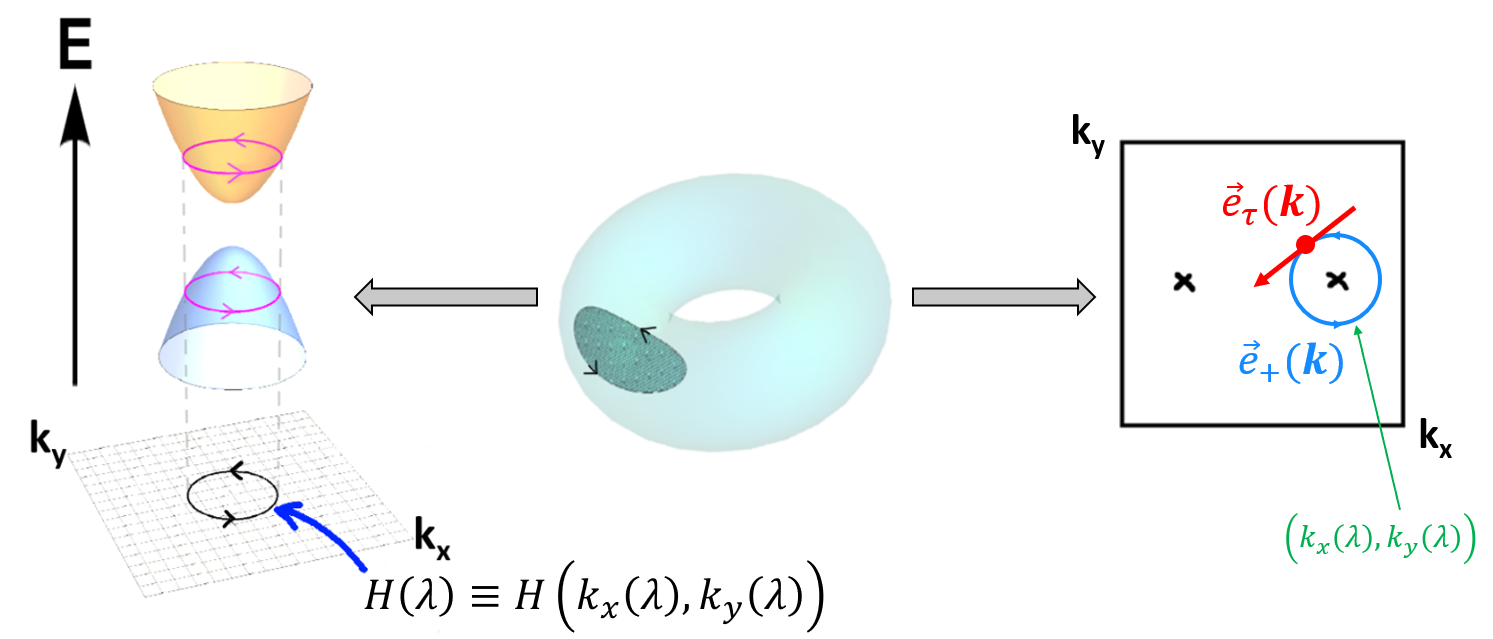
The -dependent form in Eq. (3) makes it clear that the vector may be replaced by an appropriate vector that preserves a winding property of the matrix element . Therefore, we introduce another physically-useful formulation of the interband index in terms of the chiral unit vectors (see Fig. 1):
| (4) |
All the terms in the definitions of the interband index work together to
give a quantized, gauge-invariant quantity.
III Gauge-invariant optical selection rules for excitons
The chiral unit vectors are known to decompose the interband matrix element into chiral components and . These may respectively correspond to left- and right-circularly polarized photon modes ( and ) [22]. This means that the complex-valued yield two unique vector fields with possibly different winding patterns over -space. Since is the -space derivative of the Hamiltonian, we observe that the winding number of is simply the interband line integral in our chiral formulation of the interband index Eq. (4). Therefore, we rid the optical selection rules Eq. (1) of their explicit gauge-dependence by rewriting them as:
| (5) |
One could argue that the above selection rule Eq. (5) strengthens the theory of excitons due to explicit gauge-invariance.
We computationally verified Eq. (5) by calculating (and ) for the biased bilayer graphene model that is used as an example in Ref. [23]. From Ref. [23, 39, 40]:
| (6) |
where , is the interlayer hopping amplitude, is the energy gap, and we set the factor .
To calculate the winding number given by the line integral in Eq. (4), we numerically discretized a circular counterclockwise loop (see Fig. 1) around the band edge point , and used finite differences (a central difference) to compute the derivatives of the Hamiltonian . To calculate , we discretized the two-dimensional -space grid in the region inside the circular loop, and computed for each energy level the phases from both the Berry curvature and Berry connection integrals separately. For the integral, we used the standard numerical technique given in Ref. [41] to determine the phase of the product of overlap matrices around each closed rectangular path of the -space grid, but only for the rectangles inside the circular loop. The integral was obtained by summing the phases of the individual overlap matrices along each segment of each closed rectangular path. We used Python and MATLAB for our numerical simulations. Separately, we verified our results using analytic expressions for wavefunctions and derivatives using the Hamiltonian Eq. (6), using Mathematica.
Without the interlayer hopping term (i.e. ), the
biased bilayer graphene system has symmetry
and yielded and (i.e. and from Eq. (5)),
as expected in Ref. [23].
Non-zero reduces to and should give .
Using ,
we got and (i.e. and ), as expected.
However, we caution against using this reasoning
to determine which excitons show,
without first calculating
the oscillator strength explicitly. This is because the mapping involving may be many-to-one,
while the full calculation might specify a many-to-many relation in the sense that different
may result from the same (as we saw
when mapping ).
IV Conclusion
We showed how the interband index
Eq. (4) may be used to make
the gauge-dependent optical selection rules for excitons
Eq. (1)
gauge-invariant Eq. (5).
This gauge-invariance may broaden the scope
of the types of theoretical calculations that may be
done, since we now
do not need to fix the gauge or transform between
different gauges.
This may lead to fewer ambiguities in physical interpretations that stem from gauge-dependence, since
we now have a unified theoretical framework
that is consistent across different materials and models.
By this enhancement of the predictive power of theoretical models,
our new selection rules may now
allow for clearer physical insights into excitonic effects,
since they may allow for more-accurate comparisons
between theoretical simulations and experiments
(which are typically gauge-invariant).
This may lead to potentially new phenomena
and advances in material design (especially of quantum
materials possessing novel electronic and optical properties),
which may be achievable in the near-term
given today’s high rate of advances in
interband physics and topological
effects in systems like
multilayer graphene, TMDs,
Moiré heterostructures, qubits,
and even other kinds of quasiparticles that can couple with each other (e.g., excitons, magnons, polaritons, polarons, plasmons, and phonons).
These advantages may directly influence the development
of advanced materials and technologies, with potential applications in
optoelectronics, photovoltaics, quantum computing, excitonics, spintronics, and other exciting research fronts in contemporary materials science and condensed matter physics.
We acknowledge helpful discussions with Ting Cao and Di Xiao at the University of Washington.
References
- [1] Wannier, Gregory H., ”The structure of electronic excitation levels in insulating crystals”, Physical Review, vol. 52, no. 3, pp. 191, 1937.
- [2] Cohen, Marvin L and Louie, Steven G, Fundamentals of condensed matter physics, Cambridge University Press, 2016.
- [3] Koch, S. W., Kira, M., Khitrova, G., and Gibbs, H. M., ”Semiconductor excitons in new light”, Nature Materials, vol. 5, no. 7, pp. 523–531, 2006.
- [4] Martins Quintela, M. F. C., Henriques, J. C. G., Tenório, L. G. M., and Peres, N. M. R., ”Theoretical methods for excitonic physics in 2D materials”, Physica Status Solidi (b), vol. 259, pp. 2200097, 2022.
- [5] Mak, Kin Fai, Xiao, Di, and Shan, Jie, ”Light–valley interactions in 2D semiconductors”, Nature Photonics, vol. 12, no. 8, pp. 451–460, 2018.
- [6] Chu, Junwei, Wang, Yang, Wang, Xuepeng, Hu, Kai, Rao, Gaofeng, Gong, Chuanhui, Wu, Chunchun, Hong, Hao, Wang, Xianfu, Liu, Kaihui, and others, ”2D polarized materials: ferromagnetic, ferrovalley, ferroelectric materials, and related heterostructures”, Advanced Materials, vol. 33, no. 5, pp. 2004469, 2021.
- [7] Latini, Simone and Ronca, Enrico and De Giovannini, Umberto and Hübener, Hannes and Rubio, Angel, ”Cavity control of excitons in two-dimensional materials”, Nano Letters, vol. 19, no. 6, pp. 3473–3479, 2019.
- [8] Selig, Malte, Berghäuser, Gunnar, Richter, Marten, Bratschitsch, Rudolf, Knorr, Andreas, and Malic, Ermin, ”Dark and bright exciton formation, thermalization, and photoluminescence in monolayer transition metal dichalcogenides”, 2D Materials, vol. 5, no. 3, pp. 035017, 2018.
- [9] Xiao, Jun, Zhao, Mervin, Wang, Yuan, and Zhang, Xiang, ”Excitons in atomically thin 2D semiconductors and their applications”, Nanophotonics, vol. 6, no. 6, pp. 1309–1328, 2017.
- [10] Yu, Hongyi, Cui, Xiaodong, Xu, Xiaodong, and Yao, Wang, ”Valley excitons in two-dimensional semiconductors”, National Science Review, vol. 2, no. 1, pp. 57–70, 2015.
- [11] Quintela, MFC Martins and Pedersen, T Garm, ”Anisotropic linear and nonlinear excitonic optical properties of buckled monolayer semiconductors”, Physical Review B, vol. 107, no. 23, pp. 235416, 2023.
- [12] Pedersen, Thomas Garm, ”Intraband effects in excitonic second-harmonic generation”, Physical Review B, vol. 92, no. 23, pp. 235432, 2015.
- [13] Cudazzo, Pierluigi, Sponza, Lorenzo, Giorgetti, Christine, Reining, Lucia, Sottile, Francesco, and Gatti, Matteo, ”Exciton band structure in two-dimensional materials”, Physical Review Letters, vol. 116, no. 6, pp. 066803, 2016.
- [14] Galvani, Thomas, Paleari, Fulvio, Miranda, Henrique P. C., Molina-Sánchez, Alejandro, Wirtz, Ludger, Latil, Sylvain, Amara, Hakim, and Ducastelle, François, ”Excitons in boron nitride single layer”, Physical Review B, vol. 94, no. 12, pp. 125303, 2016.
- [15] Koskelo, Jaakko, Fugallo, Giorgia, Hakala, Mikko, Gatti, Matteo, Sottile, Francesco, and Cudazzo, Pierluigi, ”Excitons in van der Waals materials: From monolayer to bulk hexagonal boron nitride”, Physical Review B, vol. 95, no. 3, pp. 035125, 2017.
- [16] Grüning, Myrta and Attaccalite, Claudio, ”Second harmonic generation in h-BN and MoS2 monolayers: Role of electron-hole interaction”, Physical Review B, vol. 89, no. 8, pp. 081102, 2014.
- [17] Trolle, Mads L., Tsao, Yao-Chung, Pedersen, Kjeld, and Pedersen, Thomas G., ”Observation of excitonic resonances in the second harmonic spectrum of MoS2”, Physical Review B, vol. 92, no. 16, pp. 161409, 2015.
- [18] Gao, Shiyuan, Liang, Yufeng, Spataru, Catalin D., and Yang, Li, ”Dynamical excitonic effects in doped two-dimensional semiconductors”, Nano Letters, vol. 16, no. 9, pp. 5568–5573, 2016.
- [19] Qiu, Diana Y., Da Jornada, Felipe H., and Louie, Steven G., ”Screening and many-body effects in two-dimensional crystals: Monolayer MoS2”, Physical Review B, vol. 93, no. 23, pp. 235435, 2016.
- [20] Olsen, Thomas, Latini, Simone, Rasmussen, Filip, and Thygesen, Kristian S., ”Simple screened hydrogen model of excitons in two-dimensional materials”, Physical Review Letters, vol. 116, no. 5, pp. 056401, 2016.
- [21] Pedersen, Thomas G., Jauho, Antti-Pekka, and Pedersen, Kjeld, ”Optical response and excitons in gapped graphene”, Physical Review B—Condensed Matter and Materials Physics, vol. 79, no. 11, pp. 113406, 2009.
- [22] T. Cao, M. Wu, and S. G. Louie, ”Unifying optical selection rules for excitons in two dimensions: Band topology and winding numbers,” Physical Review Letters, vol. 120, no. 8, p. 087402, 2018.
- [23] X. Zhang, W.-Y. Shan, and D. Xiao, ”Optical selection rule of excitons in gapped chiral fermion systems,” Physical Review Letters, vol. 120, no. 7, p. 077401, 2018.
- [24] L. Ju, L. Wang, T. Cao, T. Taniguchi, K. Watanabe, S. G. Louie, F. Rana, J. Park, J. Hone, F. Wang, et al., ”Tunable excitons in bilayer graphene,” Science, vol. 358, no. 6365, pp. 907-910, 2017.
- [25] Leung, Kevin and Whaley, K. B., ”Electron-hole interactions in silicon nanocrystals”, Physical Review B, vol. 56, no. 12, pp. 7455, 1997.
- [26] Albrecht, Stefan, Reining, Lucia, Del Sole, Rodolfo, and Onida, Giovanni, ”Ab initio calculation of excitonic effects in the optical spectra of semiconductors”, Physical Review Letters, vol. 80, no. 20, pp. 4510, 1998.
- [27] Benedict, Lorin X., Shirley, Eric L., and Bohn, Robert B., ”Optical absorption of insulators and the electron-hole interaction: An ab initio calculation”, Physical Review Letters, vol. 80, no. 20, pp. 4514, 1998.
- [28] Rohlfing, Michael and Louie, Steven G., ”Electron-hole excitations and optical spectra from first principles”, Physical Review B, vol. 62, no. 8, pp. 4927, 2000.
- [29] Onida, Giovanni, Reining, Lucia, and Rubio, Angel, ”Electronic excitations: density-functional versus many-body Green’s-function approaches”, Reviews of Modern Physics, vol. 74, no. 2, pp. 601, 2002.
- [30] Boyd, R. W., Nonlinear Optics, 3rd ed., Elsevier Science Publishing Co., Inc., New York, 2008.
- [31] Yu, P. Y. and Cardona, M., Fundamentals of Semiconductors: Physics and Materials Properties, Springer, New York, 2010.
- [32] Chang, Yu-Tzu and Chan, Yang-Hao, ”Diagrammatic approach to excitonic effects on nonlinear optical response”, Physical Review B, vol. 109, no. 15, pp. 155437, 2024.
- [33] Xu, Yang, Kang, Kaifei, Watanabe, Kenji, Taniguchi, Takashi, Mak, Kin Fai, and Shan, Jie, ”A tunable bilayer Hubbard model in twisted WSe2”, Nature Nanotechnology, vol. 17, no. 9, pp. 934–939, 2022.
- [34] Cai, Jiaqi, Anderson, Eric, Wang, Chong, Zhang, Xiaowei, Liu, Xiaoyu, Holtzmann, William, Zhang, Yinong, Fan, Fengren, Taniguchi, Takashi, Watanabe, Kenji, and others, ”Signatures of fractional quantum anomalous Hall states in twisted MoTe2”, Nature, vol. 622, no. 7981, pp. 63–68, 2023.
- [35] R. J. Elliott, ”Intensity of optical absorption by excitons,” Physical Review, vol. 108, no. 6, p. 1384, 1957.
- [36] Xiao, Di, Chang, Ming-Che, and Niu, Qian, ”Berry phase effects on electronic properties”, Reviews of Modern Physics, vol. 82, no. 3, pp. 1959–2007, 2010.
- [37] T. Fernando and T. Cao, ”Quantized interband topological index in two-dimensional systems,” Physical Review B, vol. 108, no. 8, p. L081111, 2023.
- [38] C. Xu, J. Wu, and C. Wu, ”Quantized interlevel character in quantum systems,” Physical Review A, vol. 97, no. 3, p. 032124, 2018.
- [39] C.-H. Park and S. G. Louie, ”Tunable excitons in biased bilayer graphene,” Nano Letters, vol. 10, no. 2, pp. 426-431, 2010.
- [40] E. McCann and V. I. Fal’ko, ”Landau-level degeneracy and quantum Hall effect in a graphite bilayer,” Physical Review Letters, vol. 96, no. 8, p. 086805, 2006.
- [41] T. Fukui, Y. Hatsugai, and H. Suzuki, ”Chern numbers in discretized Brillouin zone: efficient method of computing (spin) Hall conductances,” Journal of the Physical Society of Japan, vol. 74, no. 6, pp. 1674-1677, 2005.