Understanding the Local Geometry of Generative
Model Manifolds

Abstract

Deep generative models learn continuous representations of complex data manifolds using a finite number of samples during training. For a pre-trained generative model, the common way to evaluate the quality of the manifold representation learned, is by computing global metrics like Fréchet Inception Distance using a large number of generated and real samples. However, generative model performance is not uniform across the learned manifold, e.g., for foundation models like Stable Diffusion generation performance can vary significantly based on the conditioning or initial noise vector being denoised. In this paper we study the relationship between the local geometry of the learned manifold and downstream generation. Based on the theory of continuous piecewise-linear (CPWL) generators, we use three geometric descriptors – scaling ($\psi$), rank ($\nu$), and complexity ($\delta$) – to characterize a pre-trained generative model manifold locally. We provide quantitative and qualitative evidence showing that for a given latent, the local descriptors are correlated with generation aesthetics, artifacts, uncertainty, and even memorization. Finally we demonstrate that training a reward model on the local geometry can allow controlling the likelihood of a generated sample under the learned distribution.

a rhodesian ridgeback with

a city in the background

$\rho=0$                    $\rho=1$                    $\rho=1.5$

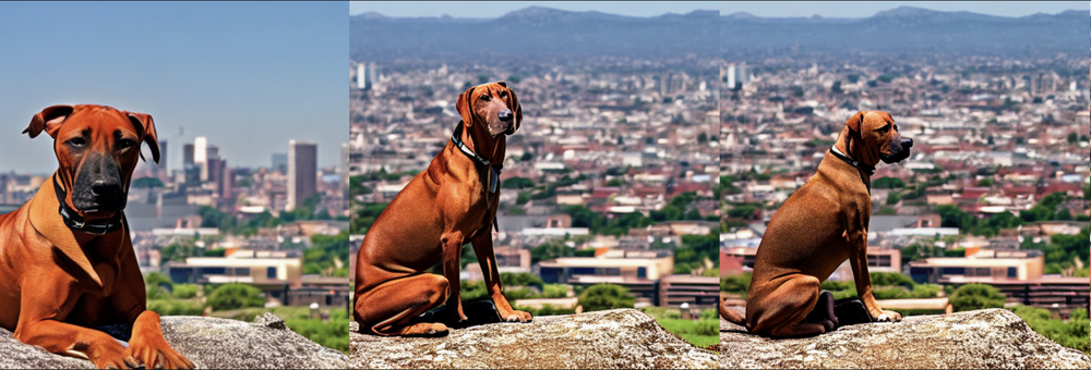
a beagle with a city

in the background

$\rho=0$                    $\rho=-1$                    $\rho=-1.5$

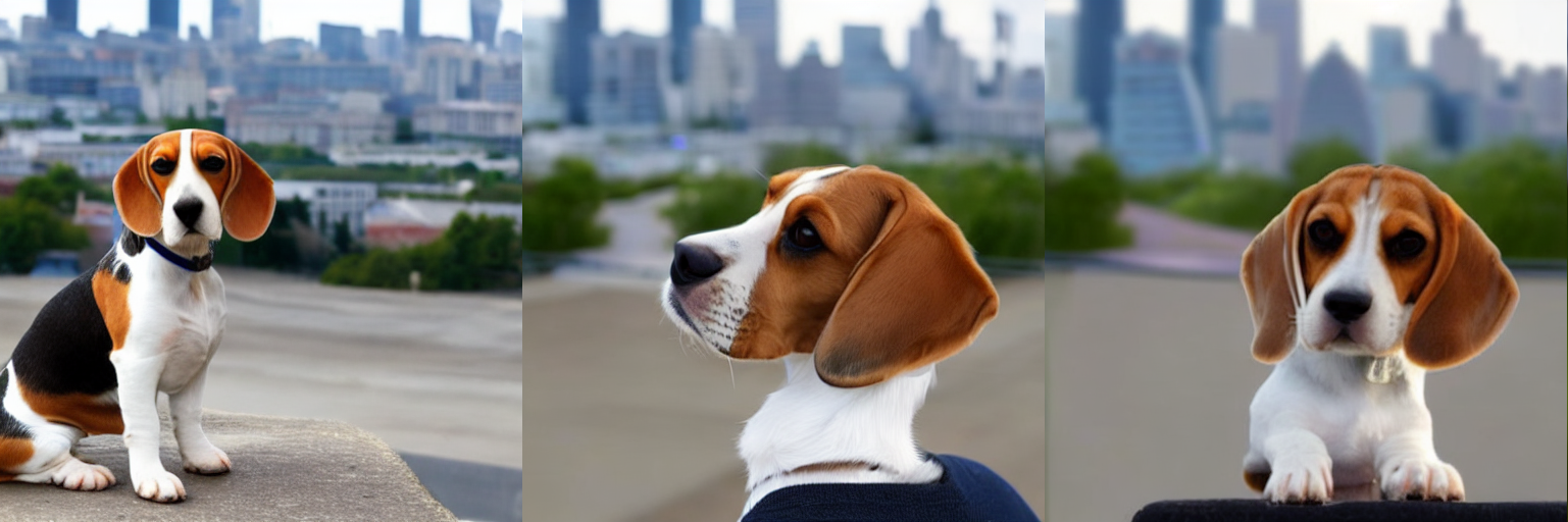
Figure 1: Controlling sampling diversity using geometry guidance. We train a reward model on the geometric descriptor local scaling computed for the decoder of Stable Diffusion [22]. Positive (top-row) or negative guidance $\rho$ (bottom-row) via this reward model allows decreasing (top-row) or increasing (bottom-row) the likelihood of the generated samples under the learned distribution. As we decrease likelihood more background elements come into view and the focus on the subject decreases, vice-versa when increasing the likelihood.

Latent Domain, $Z\in\mathbb{R}^{2}$

Data Manifold, $\text{Im}(\mathcal{G})\in\mathbb{R}^{3}$

$z\sim U(Z)$

$x=\mathcal{G}(z)$

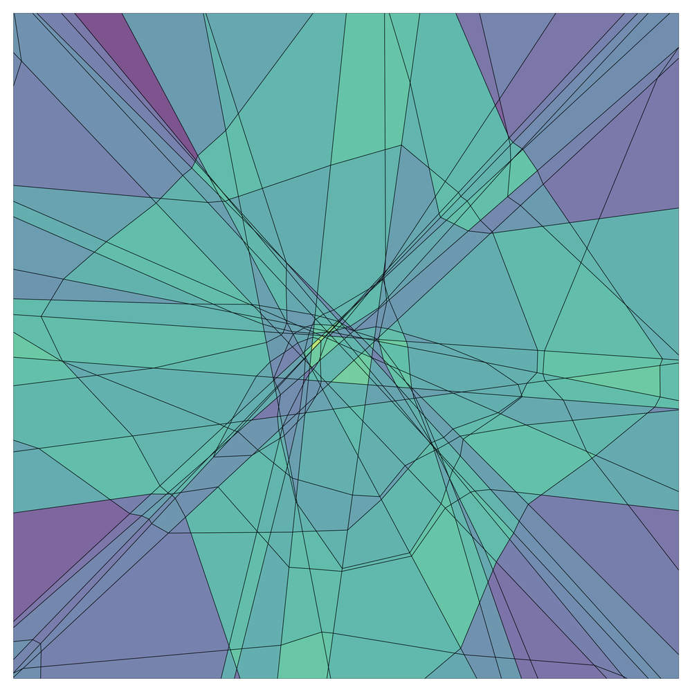
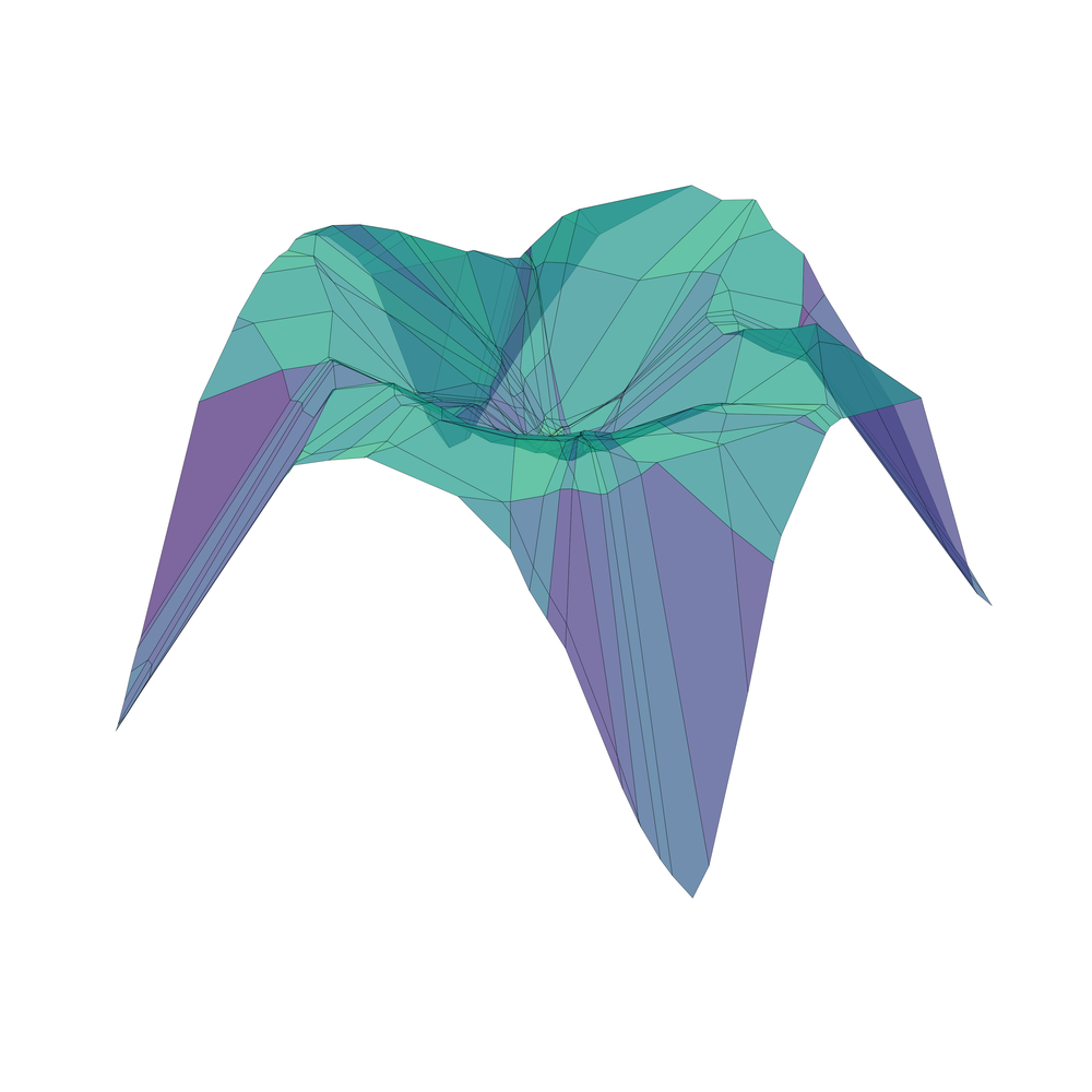
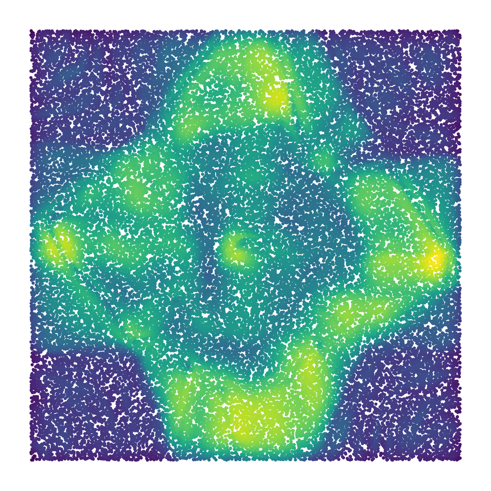
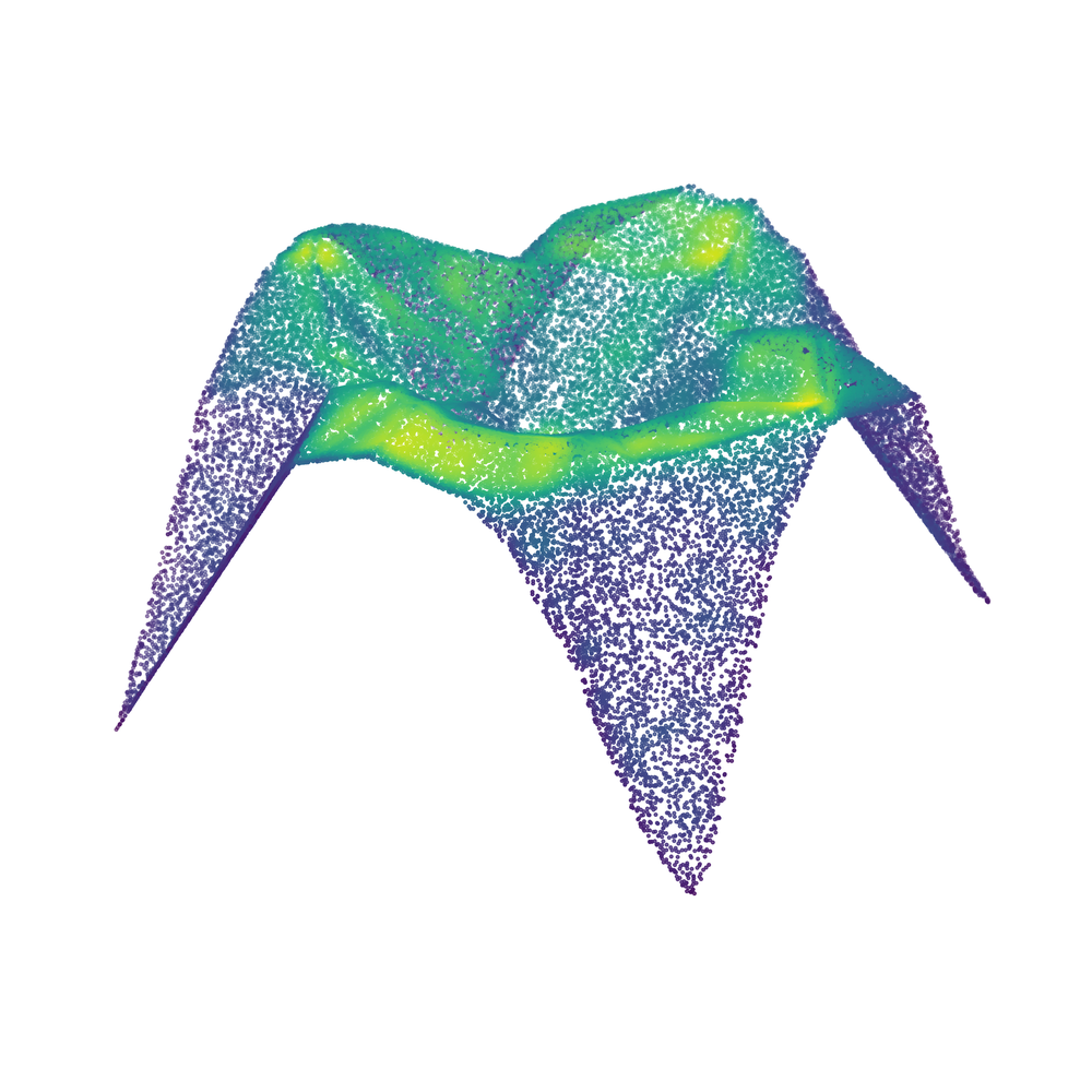
Figure 2: Exact geometry of a CPWL manifold. For a toy continuous piece-wise linear (CPWL) generator $\mathcal{G}:\mathbb{R}^{2}\rightarrow\mathbb{R}^{3}$, we provide analytically computed visualization of the input space partition, i.e., arrangement of linear regions (left) and learned CPWL manifold (middle-left). Each piece for this example, is colored by the piecewise-constant scaling induced by $\mathcal{G}$ that is analytically computed. Uniform samples from the latent domain (middle-right) and generated samples (right) are presented, colored by the estimated density at each sample using a gaussian kernel density estimator in $\mathbb{R}^{3}$. We see that for any sample $z\in\omega$, the estimated density ($\uparrow$ green) is inversely proportional with the scaling ($\downarrow$ green) for region $\omega$.

1 Introduction

In recent years, deep generative models have emerged as a powerful tool in machine learning, capable of synthesizing realistic data across diverse domains [15, 16, 22]. With the rapid increase in generation performance of such generative models, we have seen a demand for more fine-grained methods for evaluation. For example, global metrics of generation such as Fréchet Inception Distance (FID) are sensitive to both the fidelity and diversity of generated samples – precision and recall [23] were proposed to disentangle these two factors and quantify them separately. With the advent of foundational generative models like Stable Diffusion [22], human evaluation of images in a fine-grained manner has become the modus operandi for evaluation. In such cases, evaluating generative models extend beyond assessing mere sample fidelity and conditional alignment, to broader concerns about bias and memorization/duplication. The trend therefore shows a strong need for fine-grained understanding of the generative model behavior apart from what we can derive from global generation metrics. In this paper we look for answers to the following question:

Question.

For any sample generated using a pre-trained generative model, how is the local geometry of the learned manifold related to qualitative aspects of the sample?

We believe this question is especially significant 1) for models trained with large heterogeneous data distributions. Due to the heterogeneity, generation performance can vary significantly based on the sampling rate of the data manifold when training data is prepared. 2) For any pre-trained generative model without access to the training distribution, since computing global metrics like FID, precision or recall require the training data as ground truth.

How do we characterize the learned manifold?

To answer the question above, we require methods to derive local characteristics of a pre-trained generative model manifold for any given latent-sample pair $\{\bm{z},\bm{x}\}$. A large class of generative models – comprised of convolutions, skip-connections, pooling, or any continuous piece-wise linear (CPWL) operation – fall under the umbrella of CPWL generative models. Any CPWL operator, can be characterized exactly in-terms of the 1) knots/regions in the input space partition of the CPWL operator, where every knot denotes the location of a second-order change in the function and 2) the region-wise linear/affine operation, which scales, rotates, and translates any input region while mapping it to the output [1]. We therefore propose using the three geometric descriptors to characterize the learned manifold of a CPWL generator:

• Local rank ($\nu$), that characterizes the local dimensionality of the learned manifold around $x$.

• Local scaling ($\psi$), that characterizes the local change of volume by the generative model for an infinitesimal volume around $z$.

• Local complexity ($\delta$), that approximates the smoothness of the generative model manifold in terms of second order changes in the input-output mapping.

Geometric descriptors such as local scaling, complexity or rank of Deep Neural Networks, have previously been used to measure function complexity [8] and expressivity [19, 20], to evaluate the quality of representations learned with a self-supervised objective [6], for interpretability and visualization of DNNs, [10], to understand the learning dynamics in reinforcement learning [4], to explain grokking, i.e., delayed generalization and robustness in classifiers [13], increase fairness in generative models [11], control sampling in generative models [12], and maximum likelihood inference in the latent space [18].

Our contributions.

In this paper, through rigorous experiments on large text-to-image latent diffusion models and smaller generative models, we demonstrate the correlation between the local geometric descriptors with generation aesthetics, diversity, and memorization of examples. We provide insights into how these manifest for different sub-populations under the generated distribution. We also show that the geometry of the data manifold is heavily influenced by the training data which enables applications in out-of-distribution detection and reward modeling to control the output distribution. Our empirical results present the following major observations, which can also be considered novel contributions of this paper:

• C1. The local geometry on the generative model manifold is distinct from the off manifold geometry. Local scaling and local rank are indicative whether a $\{z,x\}$ pair is out-of-distribution.

• C2. A strong relationship exists between the geometric descriptors and generation fidelity, aesthetics, diversity amd memorization in large text-to-image latent diffusion models.

• C3. By training a surrogate model on the local geometry of Stable Diffusion, we can perform reward guidance to increase/decrease sampling uncertainty.

The paper is organized as follows: In Sec. 2 we define the local descriptors from first principles of CPWL generators. In Sec.3 we first show that for a toy DDPM [9] C1. holds. Following that we present visual and quantitative results showing C1. for Stable Diffusion. We also provide qualitative evidence for C2. for samples from the real Imagenet manifold. In Sec. 3.3.4 we draw connections between the local descriptors and 1) generation quality 2) uncertainty, and 3) memorization for Stable Diffusion. Finally in Sec. 4 we demonstrate how local geometry can be used as a reward signal to guide generation, providing evidence for C3.

2 Geometric Descriptors of the Learned Data Manifold

2.1 Continuous Piecewise-Linear Generative Models

Consider a generative network $\mathcal{G}$, which can be the decoder of a Variational Autoencoder (VAE) [17], the generator of a Generative Adversarial Network (GAN) [7] or an unrolled denoising diffusion implicit model (DDIM) [24]. Suppose, $\mathcal{G}:\mathbb{R}^{E}\rightarrow\mathbb{R}^{D}$ is a deep neural network with $L$ layers, input space dimensionality $E$ and output space dimensionality $D$. For any such generator, if the layers comprise affine operations such as convolutions, skip-connections, or max/avg-pooling, and the non-linearities are continuous piecewise-linear such as leaky-ReLU, ReLU, or periodic triangle, then the generator is a continuous piecewise-linear or piecewise-affine operator [1, 10]. This implies that the $\mathcal{G}:\mathbb{R}^{E}\rightarrow\mathbb{R}^{D}$ mapping can be expressed in terms of a subdivision of the input space into linear regions $\Omega$ and each region $\omega$ being mapped to the output data manifold via an affine opearation. The continuous data manifold or image of the generator $\text{Im}(\mathcal{G})$ can be written as the union of sets:

$$\text{Im}(\mathcal{G})=\bigcup_{\forall\omega\in\Omega}\{\bm{A}_{\omega}z+\bm{b}_{\omega}\forall z\in\omega\},$$ (1)

where, $\Omega$ is the partition of the latent space ${\mathbb{R}}^{E}$ into continuous piecewise-linear regions, $\bm{A}_{\omega}$ and $\bm{b}_{\omega}$ are the slope and offset parameters of the affine mapping from latent space vectors $z\in\omega$ to the data manifold. For the class of continuous piecewise-linear (CPWL) neural network based generative models, $\Omega$, $\bm{A}_{\omega}$, and $\bm{b}_{\omega}$ are functions of the neurons/parameters of the network. For a generator with $L$ layers, $\bm{A}_{\omega}$ and $\bm{b}_{\omega}$ can be expressed in closed-form in terms of the weights and the region-wise activation pattern of neurons for each layer. We refer the readers to Lemma 1 of [10] for details.

2.2 Local Geometry of Continuous Piecewise-Linear Generative Models

For any CPWL function, the input-output mapping can be expressed in terms of the input space subdivision $\Omega$ and the set of piecewise-affine parameters $\{\bm{A}_{\omega},\bm{b}_{\omega}\forall\omega\in\Omega\}$. In this section, we discuss how the local properties of the manifold can also be defined in terms of the regions $\omega$ or the region-wise affine parameters.

2.2.1 Local complexity, $\delta$

For CPWL functions, a general notion of complexity is based on the number of intervals or pieces of the function. For CPWL neural networks, a similar notion of complexity based on number of linear regions was proposed by [8]. We define local complexity of a CPWL generator as the following.

Definition 1. For a CPWL generator with input partition $\Omega$, the local complexity $\delta_{z}$ for a $P$-dimensional neighborhood of radius $r$ around latent vector $\bm{z}$ is

$$\delta_{\bm{z}} =\sum_{\forall\omega\cap V_{\bm{z}}\neq\emptyset}\mathds{1}_{\omega}$$ (2)

$$\text{where }V_{\bm{z}} =\{\bm{x}\in{\mathbb{R}}^{E}:||\mathbf{B}(\bm{x}-\bm{z})||_{1}<r\}.$$ (3)

Here, $\mathbf{B}$ is an orthonormal matrix of size $P\times E$ with $P\leq E$, $||.||_{1}$ is the $\ell_{1}$ norm operator and $r$ is a radius parameter denoting the size of the locality to compute $\delta$ for. The sum over regions $\omega\in V_{\bm{z}}$ requires computing $\Omega\cap V_{\bm{z}}$ which can be computationally intractable for high dimensions. A proxy for computing the partition for $V_{\bm{z}}$ with small $r$ is counting the number of non-linearities within $V_{\bm{z}}$, since for small $r$, the one can assume that the non-linearities do not fold inside $V_{\bm{z}}$, therefore providing an upper bound on the number of regions according to Zaslavsky’s Theorem [26]. To compute local complexity, we use the method described in [13] to estimate the number of knots intersecting $V_{\bm{z}}$.

Local complexity of CPWL neural networks have previously been connected to the expressivity of Deep Neural Networks [8, 21]. From a geometric standpoint local complexity tells us the smoothness of the learned function for a given locality. While local complexity is defined in terms of the neighborhood of a latent vector $\bm{z}$, in this paper we use it interchangeably with the local complexity of the data manifold around point $\bm{x}=\mathcal{G}(\bm{z})$.

2.2.2 Local scaling, $\psi$

Definition 2.

For a CPWL manifold produced by generator $\mathcal{G}$, the local scaling $\psi_{\omega}$ is constant for every region $\omega$ denoting logarithm of the scaling induced by the affine slope $\bm{A}_{\omega}$ for all vectors $\bm{z}\in\omega$. Local scaling for $\omega$ can therefore be expressed as

$$\psi_{\omega} =\log(\sqrt{\det(\bm{A}_{\omega}^{T}\bm{A}_{\omega})})=\sum_{i}^{k}\text{log}(\sigma_{i})\mathds{1}_{\{\sigma_{i}\neq 0\}},$$ (4)

where, $\{\sigma_{i}\}_{i=0}^{i=k}$, are the non-zero singular values of $\bm{A}_{\omega}$.

Suppose $\mathcal{G}$ has a uniform latent distribution, meaning every region $\omega$ has a uniform probability density function at the input. Under an injectivity assumption for an input space region $\omega$ and $S=\{\bm{A}_{\omega}\bm{z}+\bm{b}_{\omega}\forall\bm{z}\in\omega\}$ the output density on $S$, $p_{S}(\bm{x})\propto\frac{1}{e^{\psi_{\omega}}}$. Therefore for an injective mapping, local scaling can be considered an un-normalized likelihood measure, where higher local scaling for any given $z\in\omega$ signals lower posterior density. For two regions $\omega\in\Omega$ and $\omega^{\prime}\in\Omega$, the difference in uncertainty can therefore be written as:

$$H_{\omega}-H_{\omega^{\prime}}=\psi_{\omega}-\psi_{\omega^{\prime}},$$ (5)

where, $H_{\omega},H_{\omega^{\prime}}$ are the conditional entropy on the manifold for input space regions $\omega$ and $\omega^{\prime}$.

2.2.3 Local rank, $\nu$.

Definition 3. For a CPWL manifold produced by generator $\mathcal{G}$, local rank $\nu_{\omega}$ is the smooth rank of the the per-region affine slope $\bm{A}_{\omega}$ and can be expressed as:

$$\nu_{\omega} =\exp\left(-\sum_{i}^{k}\alpha_{i}\log(\alpha_{i})\right)$$

$$\text{where }\alpha_{i} =\frac{\sigma_{i}}{\sum_{i}^{k}\sigma_{i}}+\epsilon.$$

Here, $\{\sigma_{i}\}_{i=0}^{i=k}$ are non-zero singular values of $\bm{A}_{\omega}$ and $\epsilon=10^{-30}$ is a constant. The local rank $\nu_{\omega}$ therefore denotes the dimensionality of the tangent space on the data manifold.

$t=0.88T$

$t=0.66T$

$t=0.44T$

$t=0.22T$

$t=0$

$z^{t}$

$\psi^{t}$

$\delta^{t}$

$\nu^{t}$

Figure 3: Local geometric descriptors $\{\psi^{t},\delta^{t},\nu^{t}\}$ computed over the input domain of a 2D toy diffusion model producing distribution $z^{t}$ via reverse diffusion at noise level $t$, for an initial $z^{T}=\mathcal{N}(\mathbf{0},\mathbf{I})$. For any input vector, descriptors are computed by conditioning the diffusion model on $t$. We see that with decreasing $t$, local scaling $\psi$ and local rank $\nu^{t}$ decreases and local complexity $\delta^{t}$ increases in the proximity of the support of $z^{0}$, i.e., the learned manifold by the diffusion model. Therefore, at any $t$ during the reverse diffusion process, we can use the local descriptors computed for lower noise scales, for example $t=0.22T$, to guide generation towards or away from $z^{0}$.

2.3 Example: Toy generator trained on a $f:\mathbb{R}^{2}\rightarrow\mathbb{R}^{3}$ task

Setup. We train a toy generator $\mathcal{G}:{\mathbb{R}}^{2}\rightarrow{\mathbb{R}}^{3}$ with depth 3 and width 20, to map the 2-dimensional latent domain $[-10,10]^{2}$ onto a toy 2-manifold in a 3-dimensional output space. We train the generator with a regression loss on a ground truth manifold defined as a mixture of five gaussian functions. In Fig. 2-left, we present analytically computed visualization [10] of the piece-wise linear manifold learned by the generator as well as the latent space partition $\Omega$ represented by dark lines. Every black line represents a non-linearity of the function that folds/bends the latent space while going from ${\mathbb{R}}^{2}$ to ${\mathbb{R}}^{3}$. Therefore, the black lines are knots of the continuous piecewise affine spline generator. Each convex region $\omega$ formed by the intersection of the black lines, is mapped to $\text{Im}(\mathcal{G})$ via per region parameters as described in Equation 1. Each region in the input and output partition is colored by $\psi_{\omega}$. We also use a kernel density estimator (KDE) to estimate the density of generated samples (right) on the data manifold for a uniform latent distribution (middle-right), and color samples with the estimated density.

Observations. After training the generator, the pre-activation zero-level sets (Fig. 2) of neurons are positioned where changes to the slope of the manifold is required. The density of linear regions, i.e., local complexity is higher in the center and lower towards the edges. $\bm{A}_{\omega}$ is full-rank $\forall\omega\in\Omega$. Contrasting the KDE estimate of density and local scaling, we can see that for higher $\psi$ (blue hue) we have lower estimated density (blue hue) and vice-versa.

3 Exploring Generative Model Manifolds using Descriptors

In this Section we will be exploring the geometry of the data manifolds learned by various generative models, e.g., denoising diffusion probabilistic models, latent diffusion models like Stable Diffusion [22].

3.1 DDPM trained on toy $f:\mathbb{R}^{2}\rightarrow\mathbb{R}^{2}$ generation task.

Setup. We train a denoising diffusion probabilistic model [9] on a toy dataset to visualize how the local geometry of the learned manifold varies with 1) de-noising steps/noise levels 2) gradient descent steps. In Fig. 3 we present the local complexity $\delta^{t}$, local scaling $\psi^{t}$ and local rank $\nu^{t}$ at timesteps $t\in\{6,17,28,39,50\}$. We consider a grid of points in the 2D data space and compute the local descriptors at each point. Note that we drop the $\omega$ notation as we don’t compute $\Omega$ and no longer compute the scaling and rank in a region-wise fashion. To obtain $\bm{A}_{\omega}$ at any vector $z\in\omega$ where $\omega$ is unknown, we can take the input-output jacobian at $z$ (see Eq. 1). We add a superscript $t$ to denote the descriptors being computed for the learned output manifold at denoising step $t$. $\psi^{t}$ and $\nu^{t}$ therefore denotes the local scaling and rank by the mapping from $t$ to $t+1$.

Observations. We see that the local complexity is higher around the support of $z^{t}$ for all noise levels $t$ and both training steps shown in Fig. 3 and Fig. 19. Both local scaling and rank are lower around the data manifold until the last few diffusion timesteps, when the variance of $\psi$ and $\nu$ diminishes. The qualitative results suggest that given two diffusion models (here one is an early checkpoint and the other is a late checkpoint), local geometry around the training data for the better trained model would have higher $\delta^{t}$, and lower $\psi^{t},\mu^{t}$.

3.2 VAE training dynamics for MNIST

Setup. We train a Variational Auto Encoder (VAE) on the MNIST dataset with width 128 and depth 5 for both encoder and decoder. We add Gaussian noise with standard deviation $\{0,0.0001,0.001,0.01,0.1\}$ to the training data. Initialization was not kept fixed. In Fig. 4, we present plots showing the training dynamics of local complexity and scaling, averaged over all test dataset points from MNIST.

$\delta$

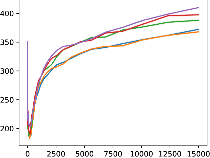
$\psi$

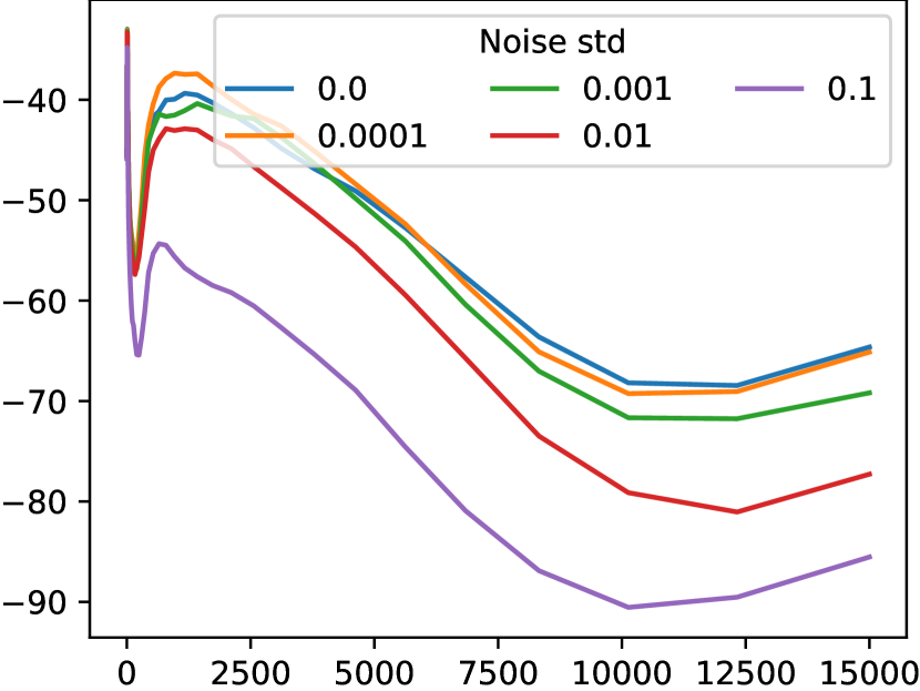
optimization steps

Figure 4: Training dynamics of geometric descriptors for a VAE trained on MNIST with additive noise. As training progresses local complexity $\delta$ increases and local scaling $\psi$ decreases suggesting an increase in expressivity and decrease in uncertainty on the data manifold. At latter time-steps, $\psi\downarrow\text{ and }\delta\uparrow\text{if noise std. is increased}$.

Observations. By increasing the noise we control the puffiness of the target manifold. We observe that as the noise standard deviation is increased there is 1) increase in $\delta$ indicating the manifold becomes less smooth 2) decrease in local scaling indicating that the uncertainty decreases. We can also observe an initial dip in both local complexity and local scaling. This is similar to what was observed for discriminative models in [13] where a double descent behavior was reported in the local complexity training dynamics of classification models. Based on these results, contrary to the observation in [13], generative models do not have a double descent in local complexity however we do observe a double ascent in local scaling. Our observations suggest that the training dynamics need to be taken into account, when comparing the local manifold geometry between two separately trained models.

3.3 Pre-trained Latent Diffusion Foundation Model

In this section we explore the local geometry of a pre-trained latent diffusion model namely Stable Diffusion v1.4 [22]. Stable Diffusion (SD) comprises of an unconditional vector quantized VAE (VQVAE) and a conditional diffusion model in the latent space of the VQVAE. The diffusion model is trained to map a gaussian distribution to the latent domain of the decoder, therefore we focus our experiments on studying the geometry of the unconditional decoder.

$\delta$

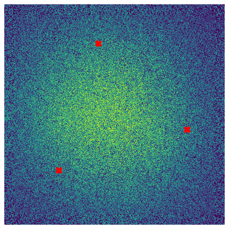
$\psi$

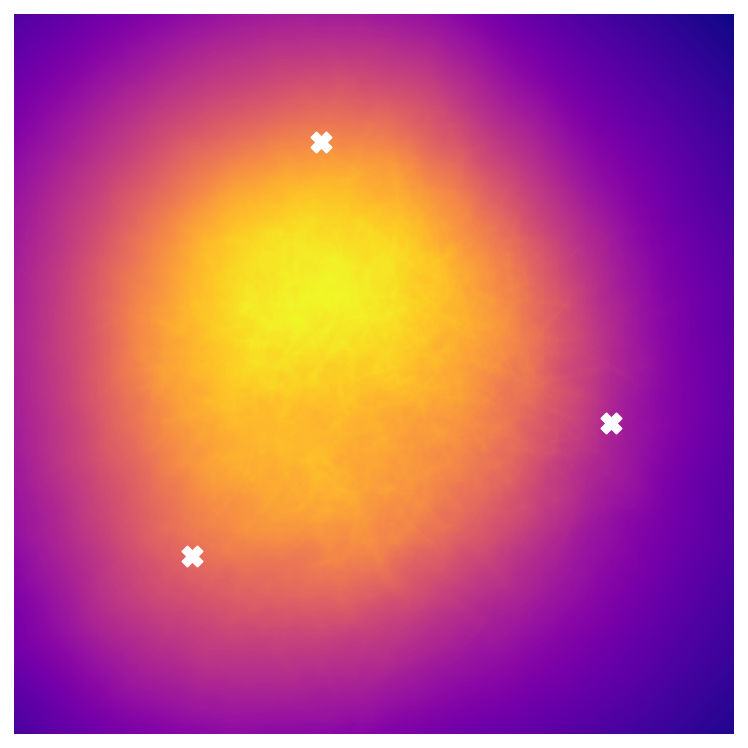
$\nu$

Anchors

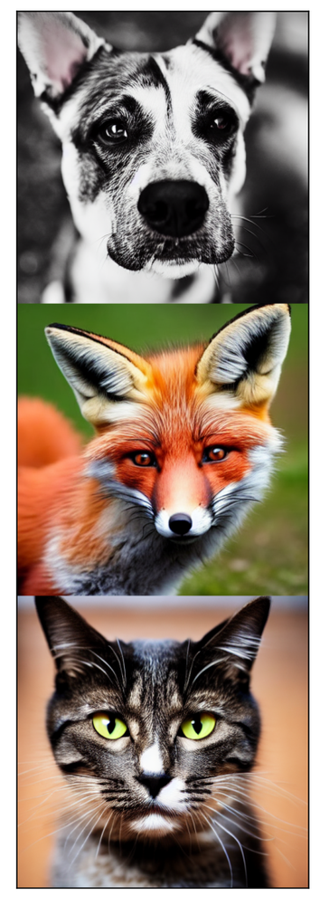
Figure 5: Geometry of the Stable Diffusion latent space. Geometric descriptors (left, middle-left, middle-right) visualized on a 2D latent space subspace, that passes through the latent representations of "a fox", "a cat" and "a dog" (right), denoted via markers on the 2D subspace descriptor. In Appendix, we provide denoised images for different high/low descriptor regions from the subspace. We see that in the convex hull of the three anchor latent vectors $\psi\uparrow$, $\nu\downarrow$ and $\delta\uparrow$. Moreover we see that in the convex hull, the local rank $\nu$ undergoes sharp changes which are not visible towards the edges of the domain.

Figure 6: Local Scaling for encoded ImageNet images. ImageNet images ordered along the columns (from left to right), with increasing local scaling $\psi$ of the Stable Diffusion decoder learned manifold. We observe that ImageNet samples with lower values of $\psi$ contain simpler backgrounds with modal representation of the object category. Conversely for higher $\psi$ we have increasing diversity both in background and foreground features.

3.3.1 Visualizing the local geometry

Setup.

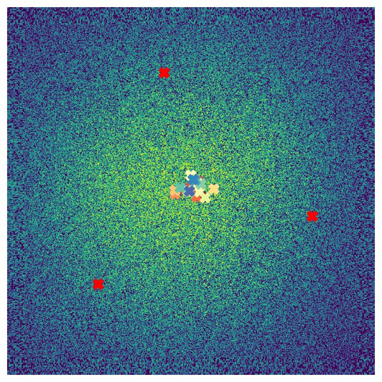
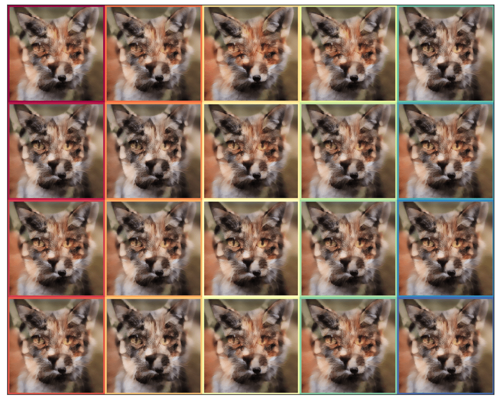
Figure 25: Decoded images (right) using $20$ latents (left) from the 2D subspace, with highest $\delta$. Each image bounding box (right) is color coded according to the corresponding latent vector (left).

We use three prompts "a cat", "a dog" and "a fox" to generate three latent vectors using the SD diffusion model. We consider a 2D slice in the latent space, going through the three denoised latents, and compute the local descriptors on a $512\times 512$ uniformly spaced grid. We compute $\delta$ for a $4$-dimensional neighborhood of radius $r=0.00001$. To make $A_{\omega}\mathds{1}_{z\in\omega}$ computation tractable, for any latent vector $z$ we take a $120$-dimensional random orthonormal projection of the SD decoder manifold [3] and compute the input-output jacobian with the projection as the output. We use a JAX implementation of Stable Diffusion on TPU resulting in $3.6s$ required for computing jointly $\delta$, $\psi$, and $\nu$ for one latent vector $z$. In Fig. 5 we present the $\delta,\psi,\nu$, on the 2D slice, along with decoded versions of the three latent vectors, used to compute the 2D slice. In Appendix Figs. 25, 26, 21, 22, 23, and  24 we present generated images from the high or low local descriptor regions from the 2D slice.

Observations.

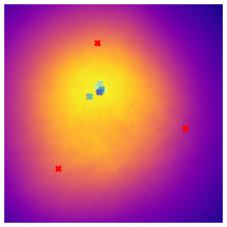
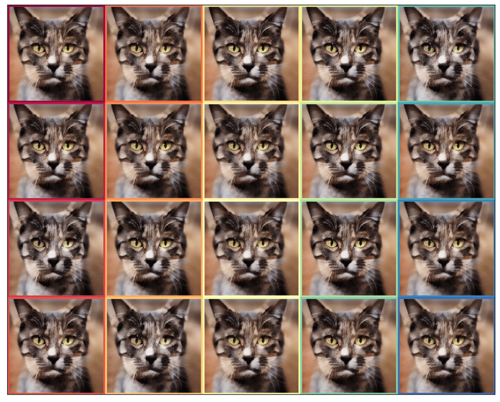
Figure 21: Decoded images (right) using $20$ latents (left) from the 2D subspace, with highest $\psi$. Each image bounding box (right) is color coded according to the corresponding latent vector (left).

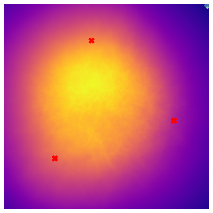
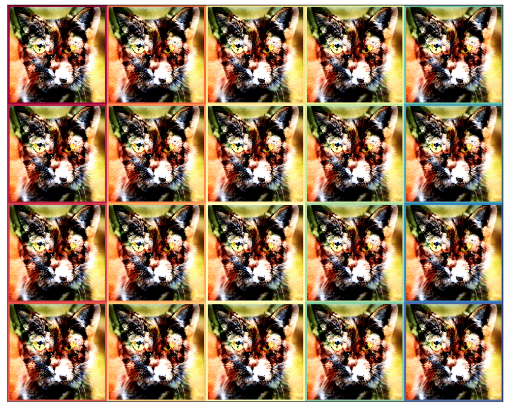
Figure 22: Decoded images (right) using $20$ latents (left) from the 2D subspace, with lowest $\psi$. Each image bounding box (right) is color coded according to the corresponding latent vector (left). Selected latents lie outside the domain of the VQGAN latent space.

Similar to what was observed for a DDPM trained on toy data (see Sec. 3.1), we observe that 1) in the convex hull of the three denoised latents, we have higher complexity indicating its proximity to the SD decoder data manifold 2) lower rank in the convex hull affirms that the convex hull has proximity to the data manifold as well. However we see a sparse collection of latents for which the rank drops further 3) as we move inside the convex hull, local scaling increases. This indicates that a convex combination of "a fox", "a cat" and "a dog" is higher uncertainty w.r.t the SD decoder. However if we move away from the convex hull we see that both $\delta$ and $\psi$ decreases while rank increases. This indicates that as we move away from the data manifold, the local scaling descriptor collapses as such regions are no longer within the support/latent domain of the SD decoder. This is further illustrated through qualitative examples in Appendix Fig. 21 and Fig. 22.

3.3.2 Local geometry of ImageNet

Setup.

Given the observations from the previous sections, we ask the question "What can local geometry of a foundation model say about a dataset?". To find an answer, we consider $20K$ samples from Imagenet with resolution higher or equal to $512\times 512$, encode the samples using the SD encoder, and study the local geometry of the SD decoder manifold for the encoded Imagenet latents. In Fig. 6 we present samples from Imagenet ordered with increasing $\psi$. In Appendix Fig. 14 we present images where the manifold dimensionality is the lowest and highest for the Imagenet samples considered.

Observations.

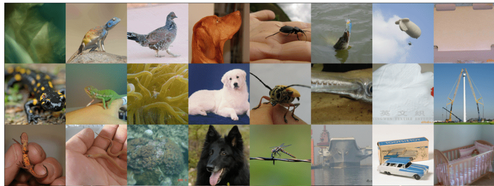
High local scaling, $\psi\uparrow$

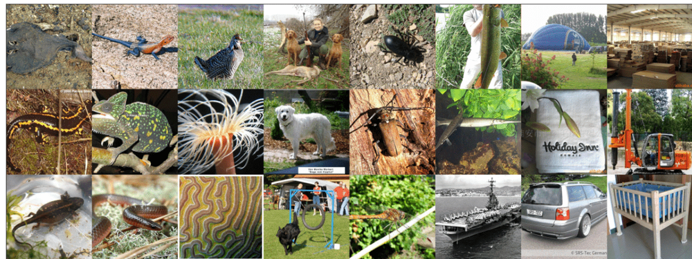
Figure 15: Imagenet images with high and low local scaling for the stable diffusion decoder. Each coordinate in both left and right image grids, correspond to the same imagenet class.

In Fig. 6 each column represents a local scaling level set, with increasing values from left to right. Recall that in Eq. 5 we show that increase in local scaling is equivalent to increase in uncertainty. In this figure, we can see that for lower uncertainty images we have more modal features in the images, i.e., the samples have less background elements and are focused on the subject corresponding to the Imagenet class. For higher uncertainty images, we see that images have more outlier characteristics. For images with higher local in Fig. 14, we see that the backgrounds have higher frequency elements compared to lower rank images. For higher rank images, the dimensionality of the manifold is higher locally, therefore allowing more noise dimensions on the manifold. In Appendix. Fig. 15 we present class-wise examples for high and low local scaling images.

Local Scaling, $\psi$

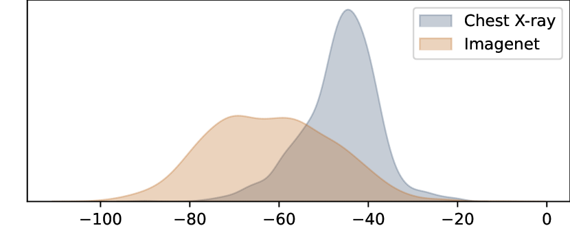
Local Rank, $\nu$

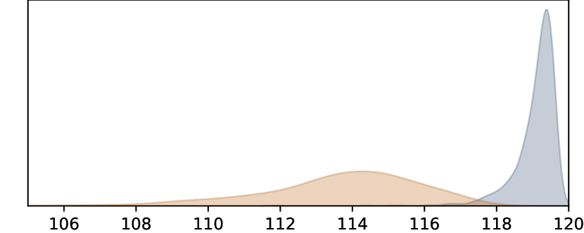
Figure 7: Geometry distinguishes out-of-distribution regions. We encode chest X-ray vs Imagenet images and present here local scaling (left) and local rank (right) distributions computed for the Stable Diffusion decoder. Here chest X-ray images are representative of out-of-distribution samples with respect to the Stable Diffusion learned distribution, and Imagenet images are considered in-distribution. We see that for OOD samples, the expected $\psi$ is higher, showing higher uncertainty under the learned distribution. The local rank is also higher for OOD samples, which correlates with our observations from Fig. 5. These results indicate that the local geometry can be used to characterize samples that are out-of-distribution with respect to a pre-trained generative model.

3.3.3 Detecting Out-of-Distribution Samples

Setup.

To study if the geometric descriptors are discriminative of out-of-distribution samples, we consider evaluating the metrics for $20K$ randomly selected Imagenet samples representing in-domain images for Stable Diffusion and $20K$ X-Ray images from the CheXpert [14] dataset representing out-of-domain images for Stable Diffusion. We present the distributions in Fig. 7.

Observations.

We see that X-ray images have higher uncertainty and higher local rank in expectation compared to Imagenet images. Especially for local rank $\nu$, Chest X-ray images from Chexpert and imagenet image distributions are almost separable. This corroborates with our visualizations from Fig. 5, where away from the convex hull of the denoised latents, we see an increase in $\nu$.

3.3.4 Relationship with Quality, Diversity & Memorization

Quality and diversity of generation for a pre-trained model, is directly connected to the estimation of the target manifold. In this section, we study the relationship between the geometric descriptors and generation quality (good estimation of the manifold), generation diversity (large support of the learned distribution) and memorization (interpolation of the target manifold at a data point).

Setup.

The experiments are organized as such:

$\bullet$ We denoise a fixed set of latent vectors using a) varying guidance scale $\{0,1,3,5,7.5,9\}$ to control quality-diversity trade-off or, b) with memorized/non-memorized prompts by Stable Diffusion. We obtain memorized prompts for SD from [25] and non-memorized prompts from the COCO dataset validation set.

$\bullet$ For a) $50K$ real ImageNet images b) $50K$ synthetic images generated by SD from increasing descriptor level sets we compute the Vendi Score [5] of clip embeddings, the aesthetic score predicted by an aesthetic reward model and a artifact reward model. For the synthetic Imagenet images, we use a guidance scale of $7.5$ and the prompt template "an image of $p$" where $p$ is a randomly class from Imagenet.

Observations.

We see in Fig. 8-bottom that for higher classifier free guidance scales during denoising, uncertainity is lower especially during the final denoising steps. This shows a clear correlation with quality since higher guidance scales result in higher quality images [22]. We also see that for higher guidance scales local rank $\nu$ is $\downarrow$ and local complexity $\delta$ is $\downarrow$ as well. For memorized prompts, in Fig. 8-top, we see that the $\psi$ is significantly lower than non-memorized prompts, indicating very low uncertainity in memorized samples compared to non-memorized samples. We also observe the manifold to be higher dimensional for memorized prompts and smoother.

Local Scaling, $\psi$

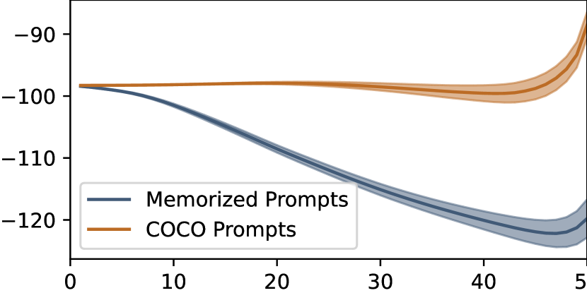
Local Rank, $\nu$

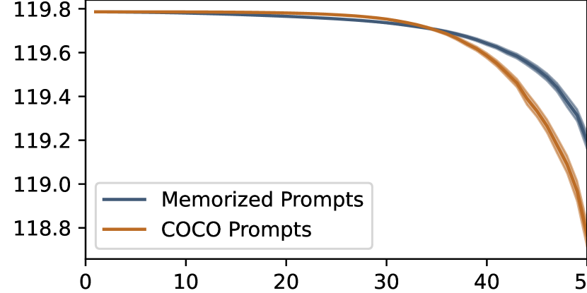
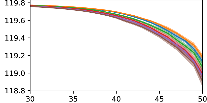
Local Complexity, $\delta$

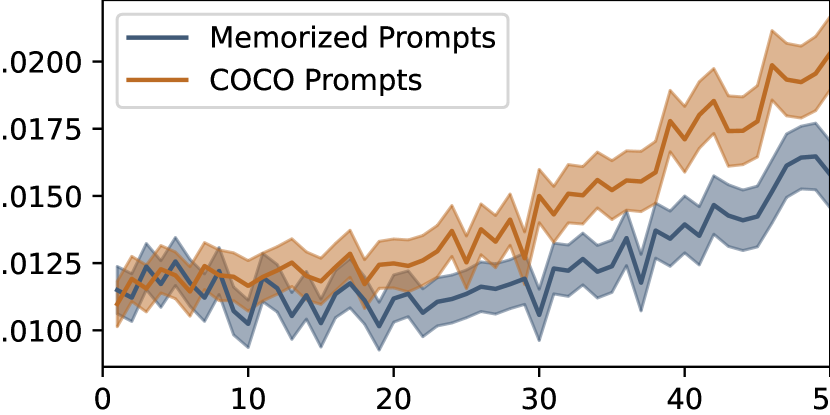
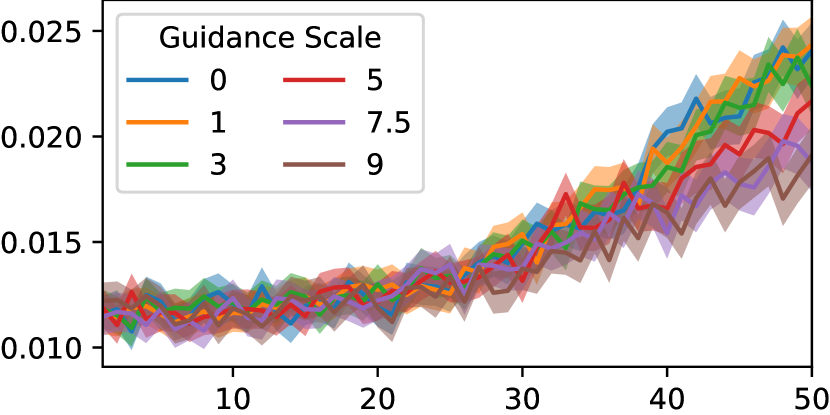
Denoising steps

Figure 8: Local geometry of denoising trajectories. Geometric descriptors computed for the VQGAN decoder, during $50$ stable diffusion denoising steps, for (top) 100 COCO and 100 memorized prompts [25] with guidance scale $7.5$ and (bottom) 100 COCO prompts with varying guidance scales. For each prompt or guidance scale, we start from the same seeds. Shaded region represents 95% confidence interval. We see that the local geometry trajectories are discriminative of memorization, as well as increased quality when stronger classifier free guidance is used.

Figure 9: Local Geometry level sets for Imagenet images. Vendi scores, Aesthetic scores and Artifact scores computed for 50k generated and real samples of ImageNet from local scaling (top) and local rank (bottom) descriptor level sets of Stable Diffusion. Scores are computed for each level set separately. Synthetic samples are generated using a guidance scale of $7.5$. We see that diversity increases for higher scaling and rank level sets for both real and synthetic data. But the aesthetic/artifact score remains more or less constant for synthetic data, since a high guidance scale is used. This shows that by using local geometry to guide generation, we can increase the diversity of generation while maintaining generation aesthetics.

In Fig.9, we see that with increasing $\psi$ and $\nu$ diversity increases, however for very high $\psi$, i.e., very uncertain images, the diversity collapses. This is due to the higher $\psi$ level sets converging towards the anti-modes of the learned distribution. We see that for real images, aesthetic and artifact scores (higher if without artifacts) get reduced for higher local scaling and rank level sets. However for generated images for higher uncertainty the rewards saturate. This is an indication that even with less perceptual/aesthetic changes, we can generate higher uncertainty images.

4 Guiding Generation With Geometry

Reward Modeling. In the previous chapters, we established that geometric descriptors are correlated with out-of-distribution detection, memorization, and aesthetics. Our primary focus has been on analyzing the geometry of the learned data manifold. In this section, we demonstrate that these geometric descriptors can be utilized to intervene in the latent representations of generative models, resulting in meaningful effects on the generated examples. Leveraging recent instance-level guidance methods, such as those described in the Universal Guidance paper [2], we can effectively influence the latents to produce significant alterations in the generated outputs. To guide the generation process, we employ local scaling as our geometric descriptor. We use classifier guidance to perform gradient ascent with step size $\rho$ on gradients derived from local scaling. This method allows us to steer the generative process by maximizing the local scaling descriptor, thus altering the generated examples in a controlled manner.

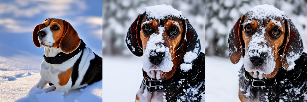
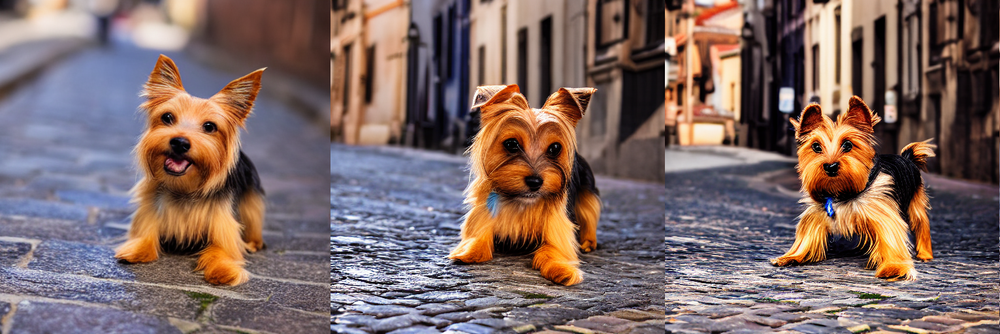
Figure 10: Reward guidance on stable diffusion (maximizing the reward). Local scale reward guidance increases from left to right in each picture, with the first image showing no reward guidance. We observe maximizing the reward leads to sharper details, improved sharpness and contrast, and higher diversity in the images. Prompts used for generation from top to bottom: “a Rhodesian ridgeback with a city in the background”, “a Beagle in the snow”, “a Australian terrier on a cobblestone street”

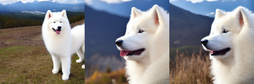
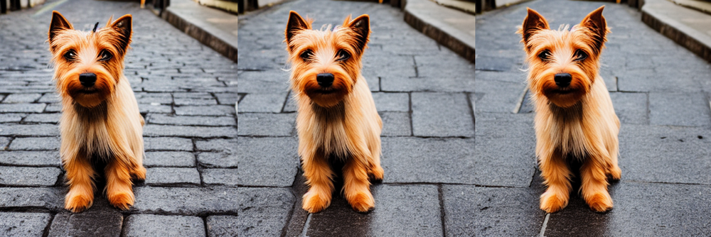
Figure 11: Reward guidance on stable diffusion (minimizing the reward). Local scale reward guidance decreases from left to right in each picture, with the first image showing no reward guidance. We observe that decreasing the local scale leads to minimized uncertainty, resulting in a noticeable blurring effect and loss of details in the image. Prompts used for generation from top to bottom:“a Beagle with a city in the background”, “a Samoyed with a mountain in the background”, “a Australian terrier on a cobblestone street”.

To enable universal guidance, we need to compute the gradient of the reward function. In our context, this entails calculating the Hessian matrix, which is computationally expensive. Instead, we train a reward model to approximate local scaling, given noisy latents at time step $t$ of the diffusion chain. We transform the regression task of estimating a continuous local scaling value into a classification task by first determining the maximum and minimum range of local scaling values for the ImageNet dataset. We then discretize this range into five uniform bins. Our training data collection process is as follows: For each image in the ImageNet dataset, we sample 10 time steps, apply noise to the encoded latents according to the sampled time step, and compute the corresponding local scaling. Subsequently, we train a classification model on pairs of latents and their associated local scaling bins.

Our experiments reveal that maximizing local scaling in the manifold of a stable diffusion model directly correlates with adding texture to the generated images. Moreover, this approach enhances diversity based on single images. By optimizing the local scaling descriptor, the generative model is guided towards producing more varied and textured outputs. This approach is notable because traditional methods for diversity guidance generally function at the distribution level. Our method, however, focuses on maximizing the inherent diversity as preserved by the model within its learned manifold, effectively steering the generated images towards the extremities of the distribution. This instance-level intervention allows for a more detailed and precise enhancement of diversity, presenting a novel approach to guiding generative models.

As seen from Fig. 10 maximizing the reward results in added details in form of sharpening the image, adding texture and contrast. We also observe that if we move towards minimizing the reward, the images tend to loose fine-grained details as seen in Fig. 20.

5 Conclusion & Future Directions

In this paper, we proposed a novel self-assessment approach to evaluate generative models using geometry-based descriptors – local scaling ($\psi$), local rank ($\nu$) and local complexity ($\delta$) - effectively while utilizing only the model’s architecture and weights. Our approach characterizes uncertainty, dimensionality, and smoothness of the learned manifold without requiring original training data or human evaluators. Our experiments demonstrated how these descriptors relate to generation quality, aesthetics, diversity, and biases. We showed that the geometry of the data manifold impacts out-of-distribution detection, model comparison, and reward modeling, enabling better control of output distribution. While using the geometry of manifolds offers a novel approach to self-assess generative models, we acknowledge two main limitations that warrant further investigation. First, the geometry of the learned manifold is inherently influenced by the training dynamics of the model. A deeper understanding of this relationship is needed to fully leverage geometric analysis for model assessment and improvement. Second, the computational complexity of our method, particularly the calculation of the Jacobian matrix, poses a practical challenge, especially for large-scale models. Future work should explore more efficient algorithms or approximations to address this limitation.

Appendix A Appendix / Supplemental material

Appendix B Broader Impact Statement

Our proposed framework for assessing and guiding generative models through manifold geometry offers several potential benefits to society. By providing a more objective and automated approach, we can significantly reduce the cost and time associated with human evaluation, making the auditing and mitigation of biases in large-scale models more accessible and efficient. This has implications for promoting fairness and equity in AI systems, particularly in domains where biases can have significant societal consequences.

Furthermore, our approach can empower researchers and practitioners to better understand the relationship between the geometry of learned representations and various aspects of model behavior, such as generation quality, diversity, and bias. This deeper understanding can inform the development of more robust and reliable generative models, leading to advancements in various fields, including art, design, healthcare, and education.

However, we recognize that our approach is not without limitations and potential risks. While it can be a valuable tool for identifying and mitigating biases, it should not and cannot fully replace human annotators, especially in high-risk domains where human judgment and contextual understanding are crucial. Our method focuses on reducing costs and improving the auditing process, but it should not be used as a standalone approach.

Moreover, the increased automation enabled by our approach raises concerns about the potential displacement of human annotators, leading to job losses and economic disruptions. While our method addresses some aspects of model evaluation, it is not comprehensive and cannot assess all facets of model behavior. Therefore, it should be used with caution and in conjunction with other evaluation methods, including human expertise.

Appendix C Extra Figures

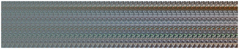
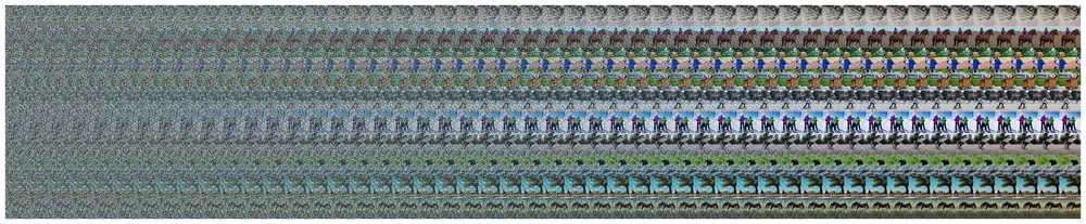
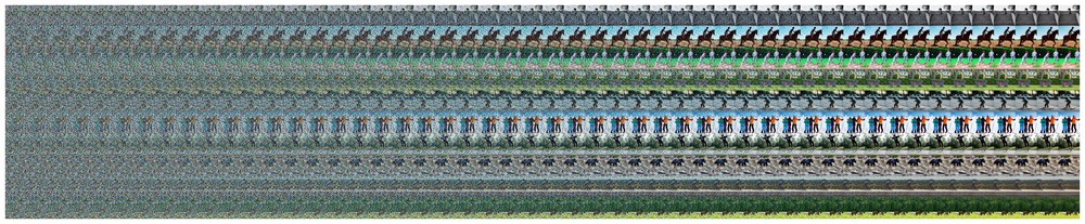
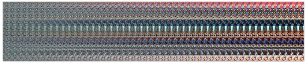
Figure 12: Images generated during 50 diffusion denoising steps for top to bottom, COCO prompts generated with guidance scale 1,5,9 and memorized prompts generated with guidance scale 7.5. Higher guidance scale images, as well as memorized images, tend to resolve faster during the denoising process.

Local scaling (log), $\psi$

Figure 13: Sub-population differences of local descriptors in generated data. Separation between the $\psi$ distributions for $1000$ images generated for each prompt in a photo of a {rich, poor} swiss person (left) and a photo of a {bartender, crane operator} (right). We see that the uncertainty as expressed by $\psi$ can vary between sub-populations indicating an underlying bias in generation diversity.

Low local rank, $\nu\downarrow$

High local rank, $\nu\uparrow$

Figure 14: Images with the lowest (left) and highest (right) local rank $\nu$ from a set of $20000$ randomly sampled ImageNet dataset samples. Low rank images contain simpler textures for every class compared to the high rank samples. This is because for images with higher local rank, the learned manifold is higher dimensional therefore allowing higher independent degrees of variations locally for the generated images.

Low local scaling, $\psi\downarrow$

Figure 16: Bivariate $(\epsilon,\psi)$ and $(\epsilon,\nu)$ distributions for training samples in green (top), and $(\delta,\psi)$, $(\nu,\psi)$ distributions for training in green and generated samples in red (bottom). Local complexity $\delta$ exhibits linear correlation with $\epsilon$ and $\psi$. Lowest $\epsilon$ samples also have lowest $\delta$, indicating that good reconstruction requires linear interpolation of the data manifold. Local rank $\nu$ uncorrelated with $\epsilon$. Both $\delta$ and $\nu$ exhibit some linear relationship with $\psi$. Note that the modes of real and generated samples for the $(\psi,\delta)$ and $(\psi,\nu)$ distributions are not completely aligned.

Figure 17: Local scaling dynamics while fine-tuning a latent diffusion model on Chest-Xray images. The local scaling is computed for generated chest-xray images, where we can see a reduction of local scaling, i.e., uncertainty.

Increasing $\psi\rightarrow$

Increasing $\delta\rightarrow$

Increasing $\nu\rightarrow$

Train

Gen.

Figure 18: Geometric descriptors of the data manifold. Level sets of data manifold descriptors for a Beta-VAE trained unconditionally on MNIST. From left to right, we present training samples (top row) and generated samples (bottom row) for linearly increasing level sets of local scaling ($\psi$) from $[-80,-42]$, local complexity ($\delta$) from $[0,120]$ and local rank ($\nu$) from $[1.5,5.5]$. Not all level sets had an equal number of samples from training/generated distributions. We see that for higher $\psi$, we have more outlier samples whereas for lower $\psi$ we have modal samples. For increasing $\delta$ we see that the quality of generated samples decreases and the diversity of samples is reduced as well. For higher $\nu$ digits become more regularly shaped.

$t=6$

$t=17$

$t=28$

$t=39$

$t=50$

$z^{t}$

$\psi^{t}$

$\delta^{t}$

$\nu^{t}$

Figure 19: After 11395 optimization steps. Geometry of a diffusion model input-output mapping, trained to on a toy 2D distribution. Local scaling lower around data manifold, local complexity higher around manifold, rank is lower around manifold as well. t=50 has considerably low variance in local scaling showing that final timestep has a diminishing change of density.

Figure 20: Reward guidance on stable diffusion (maximizing the reward).

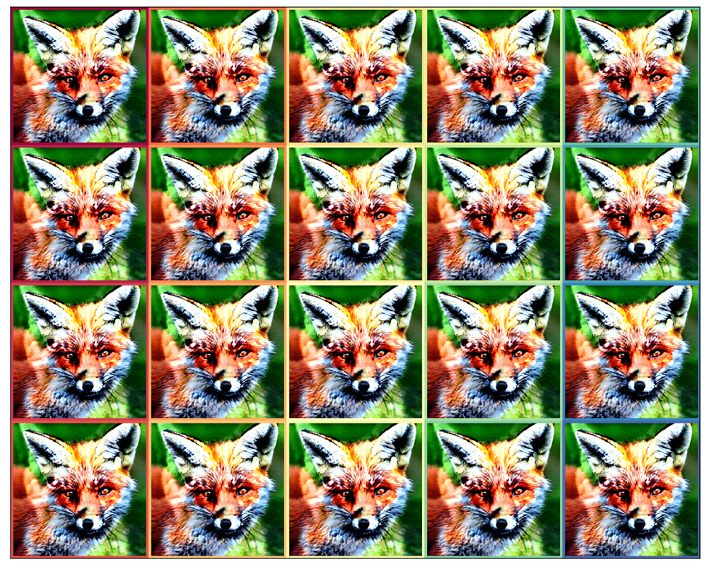
Figure 23: Decoded images (right) using $20$ latents (left) from the 2D subspace, with highest $\nu$. Each image bounding box (right) is color coded according to the corresponding latent vector (left). Selected latents lie outside the domain of the VQGAN latent space.

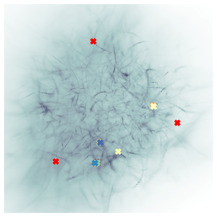
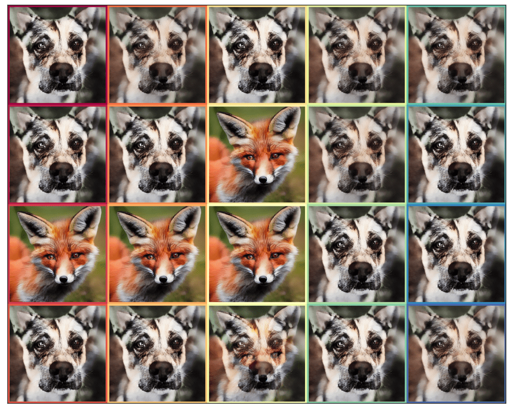
Figure 24: Decoded images (right) using $20$ latents (left) from the 2D subspace, with lowest $\nu$. Each image bounding box (right) is color coded according to the corresponding latent vector (left).

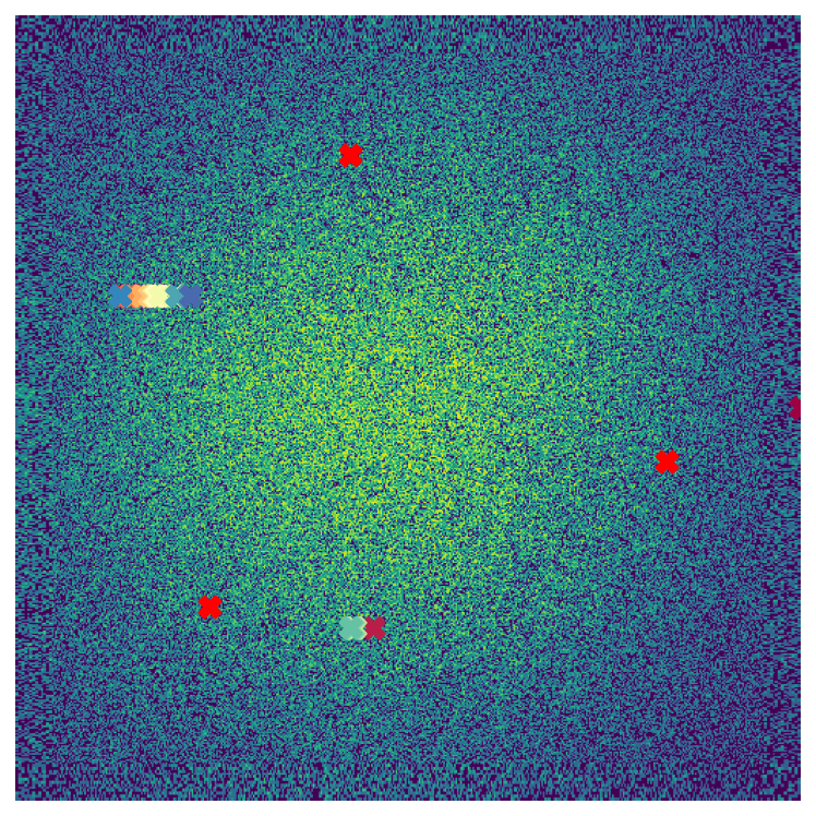
Figure 26: Decoded images (right) using $20$ latents (left) from the 2D subspace, with lowest $\delta$. Each image bounding box (right) is color coded according to the corresponding latent vector (left).

$\psi$

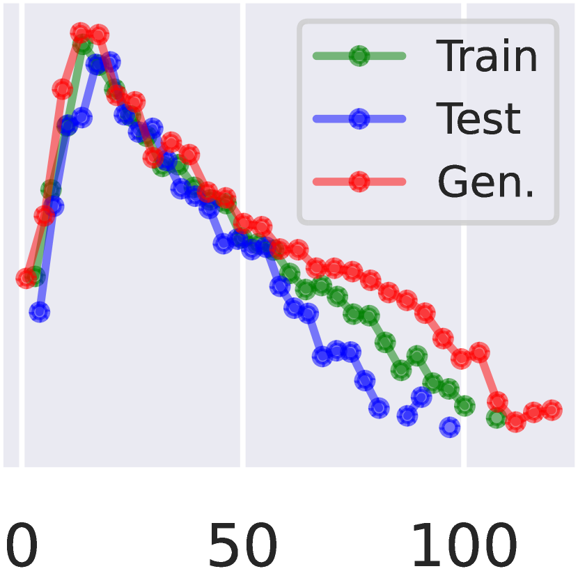
$\delta$

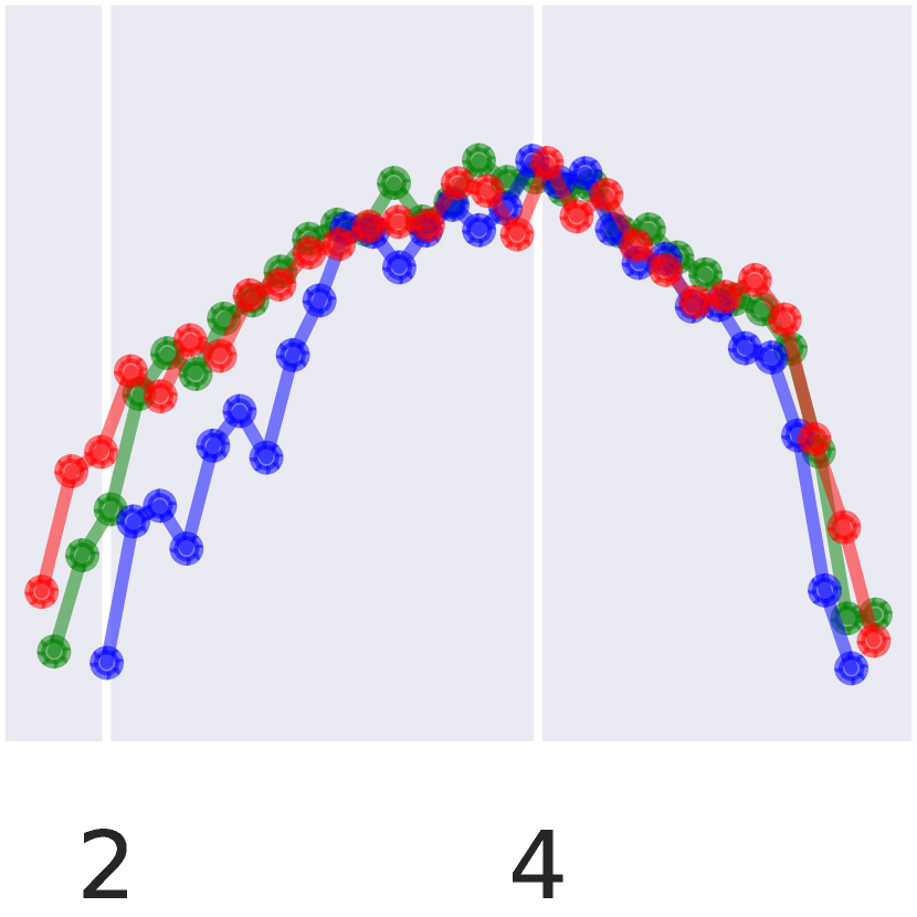
$\nu$

Figure 27: Vendi score [5] calculated for samples from different local descriptor level sets of a Beta-VAE. We take upto $150$ samples from each level set and compute vendi score seperately for the MNIST train dataset, test dataset and generated samples.

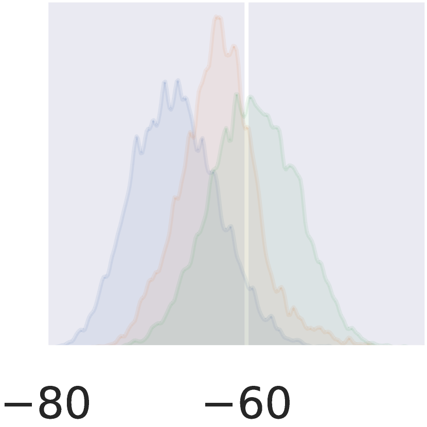
$\psi$

$\delta$

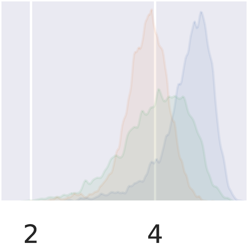
$\nu$

Figure 28: Sub-population differences of local descriptors in training data. Class-wise local descriptor distributions for a Beta-VAE trained unconditionally on MNIST. We use the VAE encoder to obtain latent vectors for the training dataset and compute descriptors using the VAE decoder. We can observe class specific separation in the distributions indicating that geometric properties may be different for different sub-populations within the training dataset.

References

- [1] Randall Balestriero et al. A spline theory of deep learning. In International Conference on Machine Learning, pages 374–383. PMLR, 2018.
- [2] Arpit Bansal, Hong-Min Chu, Avi Schwarzschild, Soumyadip Sengupta, Micah Goldblum, Jonas Geiping, and Tom Goldstein. Universal guidance for diffusion models. In Proceedings of the IEEE/CVF Conference on Computer Vision and Pattern Recognition, pages 843–852, 2023.
- [3] Richard G Baraniuk and Michael B Wakin. Random projections of smooth manifolds. Foundations of computational mathematics, 9(1):51–77, 2009.
- [4] Setareh Cohan, Nam Hee Kim, David Rolnick, and Michiel van de Panne. Understanding the evolution of linear regions in deep reinforcement learning. Advances in Neural Information Processing Systems, 35:10891–10903, 2022.
- [5] Dan Friedman and Adji Bousso Dieng. The vendi score: A diversity evaluation metric for machine learning. Transactions on Machine Learning Research, 2023.
- [6] Quentin Garrido, Randall Balestriero, Laurent Najman, and Yann Lecun. Rankme: Assessing the downstream performance of pretrained self-supervised representations by their rank. In International Conference on Machine Learning, pages 10929–10974. PMLR, 2023.
- [7] I. J Goodfellow, J. Pouget-Abadie, M. Mirza, B. Xu, D. Warde-Farley, S. Ozair, A. Courville, and Y. Bengio. Generative adversarial nets. In Proceedings of the 27th International Conference on Neural Information Processing Systems, pages 2672–2680. MIT Press, 2014.
- [8] Boris Hanin and David Rolnick. Complexity of linear regions in deep networks. arXiv preprint arXiv:1901.09021, 2019.
- [9] Jonathan Ho, Ajay Jain, and Pieter Abbeel. Denoising diffusion probabilistic models. Advances in neural information processing systems, 33:6840–6851, 2020.
- [10] Ahmed Imtiaz Humayun, Randall Balestriero, Guha Balakrishnan, and Richard G Baraniuk. Splinecam: Exact visualization and characterization of deep network geometry and decision boundaries. In Proceedings of the IEEE/CVF Conference on Computer Vision and Pattern Recognition, pages 3789–3798, 2023.
- [11] Ahmed Imtiaz Humayun, Randall Balestriero, and Richard Baraniuk. Magnet: Uniform sampling from deep generative network manifolds without retraining. In International Conference on Learning Representations, 2021.
- [12] Ahmed Imtiaz Humayun, Randall Balestriero, and Richard Baraniuk. Polarity sampling: Quality and diversity control of pre-trained generative networks via singular values. In CVPR, pages 10641–10650, 2022.
- [13] Ahmed Imtiaz Humayun, Randall Balestriero, and Richard Baraniuk. Deep networks always grok and here is why. arXiv preprint arXiv:2402.15555, 2024.
- [14] Jeremy Irvin, Pranav Rajpurkar, Michael Ko, Yifan Yu, Silviana Ciurea-Ilcus, Chris Chute, Henrik Marklund, Behzad Haghgoo, Robyn Ball, Katie Shpanskaya, et al. Chexpert: A large chest radiograph dataset with uncertainty labels and expert comparison. In Proceedings of the AAAI conference on artificial intelligence, pages 590–597, 2019.
- [15] Tero Karras, Samuli Laine, and Timo Aila. A style-based generator architecture for generative adversarial networks. In Proceedings of the IEEE/CVF Conference on Computer Vision and Pattern Recognition, pages 4401–4410, 2019.
- [16] Tero Karras, Samuli Laine, Miika Aittala, Janne Hellsten, Jaakko Lehtinen, and Timo Aila. Analyzing and improving the image quality of stylegan. In Proc. CVPR, pages 8110–8119, 2020.
- [17] Diederik P Kingma and Max Welling. Auto-encoding variational bayes. arXiv preprint arXiv:1312.6114, 2013.
- [18] Line Kuhnel, Tom Fletcher, Sarang Joshi, and Stefan Sommer. Latent space non-linear statistics. arXiv preprint arXiv:1805.07632, 2018.
- [19] Ben Poole, Subhaneil Lahiri, Maithreyi Raghu, Jascha Sohl-Dickstein, and Surya Ganguli. Exponential expressivity in deep neural networks through transient chaos. In Advances In Neural Information Processing Systems, pages 3360–3368, 2016.
- [20] Maithra Raghu, Ben Poole, Jon Kleinberg, Surya Ganguli, and Jascha Sohl Dickstein. On the expressive power of deep neural networks. In ICML, pages 2847–2854, 2017.
- [21] Maithra Raghu, Ben Poole, Jon Kleinberg, Surya Ganguli, and Jascha Sohl-Dickstein. On the expressive power of deep neural networks. arXiv preprint arXiv:1606.05336, 2016.
- [22] Robin Rombach, Andreas Blattmann, Dominik Lorenz, Patrick Esser, and Björn Ommer. High-resolution image synthesis with latent diffusion models. 2022 ieee. In CVF Conference on Computer Vision and Pattern Recognition (CVPR), pages 10674–10685, 2021.
- [23] Mehdi SM Sajjadi, Olivier Bachem, Mario Lucic, Olivier Bousquet, and Sylvain Gelly. Assessing generative models via precision and recall. arXiv preprint arXiv:1806.00035, 2018.
- [24] Jiaming Song, Chenlin Meng, and Stefano Ermon. Denoising diffusion implicit models. arXiv preprint arXiv:2010.02502, 2020.
- [25] Yuxin Wen, Yuchen Liu, Chen Chen, and Lingjuan Lyu. Detecting, explaining, and mitigating memorization in diffusion models. In The Twelfth International Conference on Learning Representations, 2024.
- [26] Thomas Zaslavsky. Facing up to arrangements: Face-count formulas for partitions of space by hyperplanes: Face-count formulas for partitions of space by hyperplanes, volume 154. American Mathematical Soc., 1975.