Simple Macroeconomic Forecast Distributions for the G7 Economies

Abstract

We present a simple method for predicting the distribution of output growth and inflation in the G7 economies. The method is based on point forecasts published by the International Monetary Fund (IMF), as well as robust statistics from the the empirical distribution of the IMF’s past forecast errors while imposing coherence of prediction intervals across horizons. We show that the technique yields calibrated prediction intervals and performs similar to, or better than, more complex time series models in terms of statistical loss functions. We provide a simple website with graphical illustrations of our forecasts, as well as time-stamped data files that document their real time character.

1 Introduction

Macroeconomic forecasts feature prominently in economic policy debates, and outlooks are often compared in the cross-section of economically similar countries across the globe. While the academic literature on macroeconomic forecasting has long appreciated the importance of measuring and communicating forecast uncertainty (as represented, e.g., by distributions and prediction intervals), the broader policy debate is still dominated by point forecasts. This may partly be due to the fact that for many countries including the Group of 7 economies (henceforth G7, including Canada, France, Germany, Italy, Japan, the United Kingdom and the United States) real-time forecast distributions are not readily available. In case of the G7 and recent editions of macroeconomic forecasting reports issued by their central banks, four of the seven reports did not explicitly quantify uncertainty. Table 1 and Appendix A provide details. Note that among the many economic organizations that issue forecasts, central banks take a leading role in terms of both societal impact and technical sophistication. If anything, we thus expect their coverage of forecast uncertainty to be more advanced than that of other economic organizations. Hence, quantitative information on macroeconomic forecast uncertainty is often unavailable, even for well-informed readers who invest the time to consult rather specialized documents.

Motivated by the discrepancy between macroeconomic forecasting in practice versus academia, we develop simple macroeconomic forecast distributions for growth and inflation in the G7 countries. These distributions are based on two main ingredients: Point forecasts provided by the International Monetary Fund (IMF), as well as appropriate quantiles from the empirical distribution of the IMF’s past forecast errors that we adjust for coherent prediction intervals across horizons. Our approach is deliberately simple and fully automatic, transparent, and based on publicly available data only. We collect all data, forecasts and prediction intervals with time stamps that document their real time character in a public GitHub repository (Becker et al., 2023). The repository also links to the website https://probability-forecasting.shinyapps.io/macropi/ where we provide graphical illustrations of all considered prospective forecasts and prediction intervals across the G7.

Transparent measurement and communication of forecast uncertainty is particularly important in economics, where forecasts are regularly used to motivate far-reaching policy decisions. In the last decades, various central bank related research initiatives have promoted probabilistic forecasting in macroeconomics. While these initiatives have inspired academic research on the topic, their impact on central bank decisions like interest rate settings has often been unclear (c.f. Conrad and Enders, 2024). For the U.S., the Survey of Professional Forecasters (SPF; Croushore and Stark, 2019) managed by the Federal Reserve Bank of Philadelphia has published probabilistic forecasts since 1968. For Europe, the ECB has maintained a similar survey since 2002 (Bowles et al., 2007). Both forecast surveys are made available in real time, following a clear release calendar. Probabilistic forecasts are available in the form of ‘histograms’, i.e., participants’ subjective probabilities for various outcome ranges (such as GDP growth between 0 and 2 percent). Given that the SPF and ECB-SPF collect forecasts (i.e., numbers) rather than forecasting methods (i.e., program code and data), the statistical techniques or judgmental components underlying the histogram-type forecasts are not known. Moreover, it is well known that the format of survey questionnaires as well as characteristics of forecasters influence the obtained results (e.g. Glas and Hartmann, 2022; Pavlova, 2024). By contrast, our forecast distributions are based on specified data inputs (IMF point forecasts, historical realizations data) and statistical techniques. Furthermore, we use a different (and arguably simpler) representation of forecast uncertainty via prediction intervals, and cover the G7 economies.

Country	Name of Central Bank	uncertainty quantified
Canada	Bank of Canada	no
France	Banque de France	no
Germany	Deutsche Bundesbank	no
Italy	Banca d’Italia	no
Japan	Bank of Japan	somewhat
United Kingdom	Bank of England	yes
United States	Federal Reserve	yes

Table 1: State of uncertainty quantification for macroeconomic forecasts that are issued by the central banks of the G7 countries. For each central bank, we consulted the “flagship” report containing forecasts for inflation and real GDP growth, often titled “Macroeconomic Projections”, “Economic Outlook” or “Monetary Policy Report” (depending on availability) and checked whether that document’s centrally communicated forecasts are accompanied by an explicit quantification of uncertainty. For more details on the reports and our protocol for extracting the information contained therein, see Section A in the appendix.

Based on work by Adams et al. (2021), a recent project by Federal Reserve Bank of New York (2024) provides probabilistic forecasts of real GDP growth, inflation and unemployment in the US. While similar in spirit, our forecast distributions are based on public data (rather than proprietary survey forecast data), and cover all G7 economies. In line with the IMF’s World Economic Outlook, our forecasts are bi-annual (rather than monthly). Furthermore, our methodology is somewhat simpler, in that we do not attempt to predict the distribution of forecast errors by means of additional variables. Schick (2024) incorporates SPF forecasts into an AR-GARCH model to forecast quantiles of U.S. GDP Growth. Reifschneider and Tulip (2019) describe prediction intervals presented by the U.S. Federal Reserve, based on root mean squared forecasting errors. The intervals’ coverage level depends on the distribution of forecast errors, amounting to roughly 70 percent under a normal distribution. Elder et al. (2005) evaluate prediction intervals implied by the Bank of England’s ‘fan charts’, which are based on a skewed distribution reflecting the Bank’s judgment. Compared to these parametric approaches, our proposed technique considers empirical quantiles of absolute forecast errors, thus avoiding restrictive functional form assumptions. The robustness of quantiles is an important advantage in turbulent times like the recent corona pandemic, whose extreme observations are handled plausibly and automatically by quantiles. By contrast, non-robust estimation methods based on squared errors are dominated by these observations. This leads to difficult questions about how to handle extreme observations in practice, with many studies resorting to ad-hoc choices of the sample period. See Lenza and Primiceri (2022) and Knüppel et al. (2023, Section 5) for further discussion.

Finally, our paper relates to a growing body of academic literature on how to construct forecast distributions of macroeconomic variables. Our proposed approach intends to be as simple as possible (in terms of data requirements and statistical techniques), subject to being reasonably competitive in terms of statistical performance. Studies like Clements (2010), Krüger (2017), Ganics et al. (2022) and Krüger and Plett (2024) indicate that forecast distributions based on past point forecast errors perform similar to, or better than, subjective histogram-type forecasts as provided by the SPF and ECB-SPF. These findings motivate our use of the IMF as an external point forecast, together with a suitable set of historical forecast errors. See Qu et al. (2024) for recent evidence on the good performance of IMF point forecasts relative to private sector survey forecasts. Compared to studies that create ‘self-contained’ forecast distributions based on multivariate time series data (see e.g. Clark et al., 2024, and the references therein), our use of the IMF as an external point forecast greatly reduces data requirements and modeling complexity. For our purposes, this simplification outweighs the inherent benefits of producing a self-contained forecast. More broadly, the principle of constructing forecast distributions based on a history of point forecasts and associated realizations has proven successful in many empirical contexts across the disciplines. Walz et al. (2024) and Angelopoulos et al. (2023) provide further discussion in the context of meteorology and machine learning, respectively.

The remainder of this paper is organized as follows. Section 2 contains methodology for computing empirical quantiles in the current setup. In particular, we discuss techniques for ensuring that forecasts are coherent across multiple horizons, as well as assumptions about the (a)symmetry of forecast errors. Section 3 describes relevant benchmark methods and presents empirical results on the forecasting performance of the proposed method. In our empirical analysis, we show that the method yields calibrated prediction intervals (with coverage close to its nominal level), and performs at least as well as the benchmarks in terms of the interval score, a statistical loss function for prediction intervals. Section 4 concludes. The appendix contains details on Table 1, as well as further empirical results and robustness checks. Replication materials for the paper are available from Becker et al. (2023).

2 Methods

2.1 Constructing Prediction Intervals

This paper aims to provide a calibrated probabilistic assessment of macroeconomic indicators in an accessible manner: First, the format of the probabilistic forecasts should be easily understandable to facilitate their communication and second, the methodology should be simple, to make the forecast generation transparent and readily reproducible.
We use prediction intervals as a method for capturing uncertainty. This format has been shown to be successful in a meteorological (Mass et al., 2009; Raftery, 2016) and public health (Bracher et al., 2021b; Cramer et al., 2022) context. While conveying less information than, for instance, a full probability distribution, they are easier to use and understand for non-statisticians: For a given confidence level $\tau\in(0,1)$, a prediction interval is represented by only two numbers $u^{\tau}>l^{\tau}$, the upper and lower endpoints of the interval.
We use an existing series of point forecasts for macroeconomic indicators, and construct a prediction interval for a given level $\tau$ around the point forecast $\hat{y}$ in the following way:

$$\begin{split}u^{\tau}&=\hat{y}+c^{u,\tau}\\ l^{\tau}&=\hat{y}+c^{l,\tau},\end{split}$$ (1)

with $c^{u,\tau}>c^{l,\tau}$. Note that $c^{l,\tau}$ can, but does not have to, be negative. To get a finer representation of the predictive distribution, one can construct these intervals for multiple levels of $\tau$. Given $\tau$, we obtain values for the upper and lower prediction bands $c^{u,\tau}\text{ and }c^{l,\tau}$ from past data on forecasts and realizations, according to the following methodology.

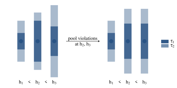
Figure 1: Illustration of the PAVA-type correction procedure of Algorithm 1 used in cases where the monotonicity constraint is not upheld across horizons. The figure shows prediction intervals for two confidence levels $\tau_{1}$ (dark blue) and $\tau_{2}$ (light blue), with $\tau_{1}<\tau_{2}$, and three horizons $h_{1}<h_{2}<h_{3}$. The prediction intervals for level $\tau_{1}$ violate the constraint (5) at horizons $h_{2}$ and $h_{3}$. As a result, prediction intervals at both levels $\tau_{1}$ and $\tau_{2}$ are pooled at $h_{2}$ and $h_{3}$, averaged, and thereafter assigned to both horizons. For illustration purposes, all forecasts were centered at the same value.

For a given country and forecast target, suppose we have access to a past series of forecasts $\{\hat{y}_{t,h}\}_{t=1,...,T}$, as well as to the corresponding realized values $\{y_{t}\}_{t=1,...,T}$. The series of forecasts must have both sufficient history and still be ongoing. The target year is indexed by $t$ and the forecast horizon by $h$. The latter denotes the time difference between the date the forecast is made (the “forecast origin”) and the end of year $t$, when the quantity realizes.
Given these forecast-observation pairs, we construct sets

$$\mathcal{E}^{abs}_{t,h}=\{\hat{e}^{abs}_{t^{*},h}|t-R\leq t^{*}<t\}$$ (2)

based on the absolute forecast errors

$$\hat{e}^{abs}_{t,h}=|y_{t}-\hat{y}_{t,h}|.$$ (3)

For a discussion of why we choose absolute forecast errors rather than raw error values, we refer to Section 2.2. In cases where $h$ is larger than one year and the directly preceding target year(s) have not yet completed, the size of the set (2) is kept fixed at $R$ by incorporating the appropriate number of previous years. Apart from practical constraints imposed by a limited sample size, the choice of $R$ reflects a trade-off between stability (which suggests a large value of $R$) and emphasizing recent observations (which suggests a small value of $R$); see e.g. Gneiting et al. (2005, Section 3).
Given (2), we obtain the lower $l$ and upper $u$ endpoints of a prediction interval of desired level $\tau$ via adding and subtracting the empirical $\tau-$quantile of (2) to the current point forecast:

$$\begin{split}u^{\tau}_{t,h}&=\hat{y}_{t,h}+q^{\tau}\left(\mathcal{E}_{t,h}\right)\\ l^{\tau}_{t,h}&=\hat{y}_{t,h}-q^{\tau}\left(\mathcal{E}_{t,h}\right),\end{split}$$ (4)

where $q^{\tau}$ refers to the empirical quantile function. Due to the monotonicity of the empirical quantile function $q^{\tau}$ in $\tau$ , quantile crossing is avoided by construction across different levels of $\tau$. Note also that we obtain a symmetric interval since here $c^{l,\tau}=-c^{u,\tau}$.
As discussed by Hyndman and Fan (1996), several methods for computing empirical quantiles are implemented in R (R Core Team, 2023) and other statistical programming environments. As detailed in Section 3.2, we will give preference to combinations of an empirical quantile method and window length $R$ that, subject to data availability and the chosen confidence levels, allow extraction of quantiles directly from the order statistics of the forecast errors in $\mathcal{E}_{t,h}$ and thus do not rely on interpolation between observed values. This choice is motivated by simplicity, in that interval endpoints that stem directly from observed forecast errors seem easier to understand.
Many economic organizations (such as the IMF) simultaneously issue forecasts for multiple future years. Here we impose the assumption that the length of prediction intervals should not decrease with the forecast horizon. This assumption is intuitively appealing, and also aligns with theoretical notions of optimal forecasting in stationary time series models (see e.g. Patton and Timmermann, 2011; Krüger and Plett, 2024). In general, a sufficient condition for the assumption is that

$$\begin{split}c^{u,\tau}_{t,h}&\leq c^{u,\tau}_{t,h^{\prime}},\textrm{ for all }h<h^{\prime},\text{ and}\\ c^{l,\tau}_{t,h}&\geq c^{l,\tau}_{t,h^{\prime}},\textrm{ for all }h<h^{\prime};\end{split}$$ (5)

for the case of a symmetric method (with $c^{l,\tau}=-c^{u,\tau}$), it is sufficient to check either one of the inequalities. We impose this restriction on the values $c^{l,\tau},c^{u,\tau}$ rather than directly on the length of the prediction interval in order to simplify the adjustment mechanism in case of violations. In particular, if monotonicity is violated, we enforce it via the pool-adjacent-violators (PAVA) type reordering outlined in Algorithm 1. See e.g. de Leeuw et al. (2009) for background on the PAVA algorithm. In short, the procedure amounts to iteratively merging predictive intervals at all confidence levels in case of violations, until the condition in (5) is upheld across all horizons. Since the PAVA type reordering is applied to all considered quantile levels if there is a violation of (5) at one level, the reordering does not cause any quantile crossing.

The initial solution is $c^{u,\tau}_{t,h}(0):=q^{\tau}\left(\mathcal{E}_{t,h}\right)$, where $q$ is the chosen empirical quantile function. The index for the blocks is $r=1,...,B$ where $B$ is initially the number of forecast horizons.

while there exists $r,\tau^{\prime}$ such that: $c^{u,\tau^{\prime}}_{t,r}(k)>c^{u,\tau^{\prime}}_{t,r+1}(k)$ do

     For all values of $\tau$: Merge $c^{u,\tau}_{t}(k)-$values from blocks $r$ and $r+1$ into block $r$ and average. Merge $c^{l,\tau}_{t}(k)-$values from blocks $r$ and $r+1$ into block $r$ and average.

end while

Algorithm 1 PAVA-type algorithm for symmetric prediction invervals.

2.2 Absolute versus Raw Errors

As noted previously, we rely on absolute errors to construct prediction intervals. We next compare absolute errors to raw,“directional” errors given by

$$\hat{e}^{d}_{t,h}=y_{t}-\hat{y}_{t,h}.$$ (6)

The relevant sets of errors $\mathcal{E}^{d}_{t,h}$ are constructed analogously and the prediction interval endpoints can be calculated as

$$u^{\tau}_{t,h} =\hat{y}_{t,h}+q^{\frac{1+\tau}{2}}\left(\mathcal{E}_{t,h}\right)$$

$$l^{\tau}_{t,h} =\hat{y}_{t,h}+q^{\frac{1-\tau}{2}}\left(\mathcal{E}_{t,h}\right).$$

A major drawback of this method is as follows: Especially when few past observations of the series are available, and with smaller confidence levels such as $\tau=0.5$, it is possible that either the $\frac{1-\tau}{2}$-quantile is positive or the $\frac{1+\tau}{2}$-quantile is negative. In particular, this means that the point forecast would not be contained in the prediction interval that is constructed “around” it. This type of one-sided behavior seems practically relevant in the empirical setup we consider below.
On the other hand, prediction intervals based on “directional” errors are entirely unrestricted, whereas the use of absolute errors (4) comes at the cost of implicitly assuming that the distribution of forecast errors is symmetric around zero (c.f. Breth, 1982). This is a rather stringent assumption. It implies that the point forecast corresponds to the median functional of the forecast distribution. Furthermore, symmetry implies that the median functional equals the mean functional. In this sense, the assumption of symmetric forecast errors sidesteps the debate about which functional of the forecast distribution is being addressed by a given point forecast (e.g. Elliott et al., 2005; Manski, 2018). From a statistical perspective, the assumption that forecast errors are symmetric around zero regularizes the estimate of the forecast error distribution. This form of regularization seems beneficial if its implied assumptions are at least approximately correct, and if the sample size is small, as is the case in our application. In the related context of estimating a conditional (rather than unconditional) distribution of forecast errors, Krüger and Plett (2024) find that imposing symmetry around zero is helpful in terms of forecasting performance.
Table 2 sketches these and further considerations for deciding between absolute versus directional errors. In view of these arguments, we opt to use absolute errors as our default option. Of course, this choice reflects a weighting of the different criteria mentioned in Table 2, which is necessarily subjective.

Absolute Errors			Directional Errors
Shape of prediction interval
$+$	Prediction intervals are centered around the existing point forecast. This may be seen as intuitive.		$-$	Prediction intervals are not centered around the point forecast and may not even contain it. Especially for intervals with a high nominal level of confidence, this may be seen as unintuitive.
Assumptions
$-$	True distribution of forecast errors must be symmetric around zero (otherwise, use of absolute errors is suboptimal in large samples). Accordingly, the external point forecast is interpreted as referring to the median functional, which coincides with the mean functional in this case.		$+$	No distributional assumption on forecast errors required. Accordingly, no assumption regarding the interpretation of the external point forecast.
$+$	Implicit symmetry assumption on distribution of forecast errors regularizes quantile estimation, which can be beneficial in small samples (c.f. Breth, 1982).		$-$	No regularization, and quantile estimation can be challenging in small samples.
In our application (Section 3): Scores and calibration
$+$	Coverage rates are close to nominal.		$-$	Interval scores are mostly similar to absolute error method, but coverage rates are often substantially below nominal rates.

Table 2: Advantages and disadvantages of using either absolute error calculation (left column) or direct error calculation (right column) for constructing forecast intervals. Advantageous points are indicated with $+$, disadvantageous points with $-$.

2.3 Assessing Forecast Accuracy

In assessing the quality of our forecasts, we follow the paradigm to ‘maximize sharpness subject to calibration’ postulated by Gneiting et al. (2007). Sharpness means that the forecast distribution should be as narrow as possible. Calibration means that the forecast distribution should be coherent with observed outcomes. In practice, there is a clear trade-off between both objectives. For example, a forecast distribution with all probability mass in one point (indicating no uncertainty) would be perfect in terms of sharpness, but likely poor in terms of calibration. In order to assess the calibration of probabilistic forecasts in an interval format, a simple method is to compare the empirical and nominal interval coverage rates. That is, a $\tau\%$ coverage interval should over time cover roughly $\tau\%$ of observations. As argued by Raftery (2016), forecasts users tend to view calibration as a crucial feature of a trustworthy forecast. A proper scoring rule can then be used to evaluate the forecast sharpness in conjunction with its calibration properties. Briefly, a scoring rule is called proper if it encourages forecasters to state what they think is the correct prediction (Winkler, 1996; Gneiting and Raftery, 2007). Given the format of our forecast, the interval score (Gneiting and Raftery, 2007) is a natural choice of scoring rule:

$$\text{IS}_{\tau}(F,y)=(u-l)+\frac{2}{1-\tau}(l-y)1(y<l)+\frac{2}{1-\tau}(y-u)1(y>u),$$ (7)

for a given confidence level $\tau$ and the corresponding prediction interval $[l,u]$ implied by the forecast distribution $F$. Here we consider scores in negative orientation, i.e., smaller scores correspond to better forecasts. The first summand of Equation (7) can be interpreted as a penalty for dispersion (i.e., lack of sharpness) of the forecast distribution, corresponding to wide prediction intervals, such that $u-l$ is large. The second summand can be seen as a penalty for overprediction, such that the outcome $y$ is smaller than the interval’s lower endpoint $l$. Conversely, the third summand of (7) represents a penalty for underprediction. Given that (weighted) sums of proper scoring rules are again proper (Gneiting and Raftery, 2007), we can average scores for different levels of $\tau=\tau_{1},\ldots,\tau_{K}$ in order to obtain a summary measure of forecast performance. In the following, we consider a weighted average with weights $w_{1},...,w_{K}$ as proposed by Bracher et al. (2021a). Specifically, we set $K=2$, $\tau_{1}=0.5$ and $\tau_{2}=0.8$, and thereby $w_{1}=\frac{1-\tau_{1}}{2}=0.25$ and $w_{2}=\frac{1-\tau_{2}}{2}=0.1$. Since we focus on generating prediction intervals, we do not incorporate the point (median) prediction into the interval score. The latter is externally provided by the IMF in our empirical setup.

3 Empirical Results for the G7 Economies

In this section, we apply the methods described in Section 2 to the IMF’s World Economic Outlook (WEO) forecasts.

3.1 Data and Forecast Targets

The WEO’s merit relative to other forecast sources has been established in studies such as Timmermann (2007) and Qu et al. (2024), which is why we consider it a promising candidate for this analysis. Started in 1990, the WEO has issued bi-annual forecasts for multiple (up to six) years into the future, for several variables including real GDP growth and inflation (International Monetary Fund, 2024). The code that downloads and processes the current WEO dataset from the IMF website is available in a public GitHub repository (Becker et al., 2023).
For both the calculation of forecast errors and the subsequent evaluation of forecasts, we use the truth values that are included in the WEO data. As is typical for macroeconomic data, these are updated over time, due to relevant information becoming available retrospectively. For example, the best estimate of GDP in the year 2022 is typically different in spring 2023 (the first WEO estimate) than in fall 2023 (the second WEO estimate). While earlier studies of the WEO, such as Timmermann (2007), choose different truth values depending on the forecast horizon, we opt for a consistent choice and mainly use the truth value that is published in the fall release following the year in question (e.g., fall 2023 for 2022). When constructing forecast intervals in spring, we however take a pragmatic approach and use the spring release’s truth value for the directly preceding year, as the fall release for this year is not available until six months later.
Our analysis focuses on the G7 economies and forecasts for the current and next year. We compute these forecasts at each bi-annual forecast date (spring and fall) covered by the IMF. This concise selection allows an accurate review and communication of results. We generally pool forecast evaluation results across the seven countries in order to increase the sample size. Of course, given the dependence of observations across countries, this step does not simply increase our effective sample size by seven.
We focus on 80% and 50% prediction intervals. As argued by Raftery (2016), an 80% interval satisfies the intuitive notion that a prediction interval should ‘typically’ cover the realizing outcome, while often being reasonably short (i.e., sharp) in practice. The $50\%$ interval is additionally constructed to provide further characterization of the forecast distribution for interested users, and to serve as a further check of the validity of the methodology.

3.2 Choice of Tuning Parameters

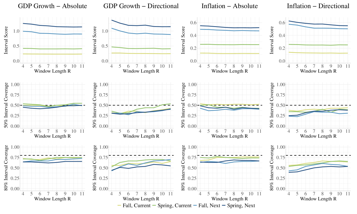
Figure 6: Interval scores and empirical coverage rates in the training sample (2001-2012), for both targets and error extraction methods, and for various choices of the rolling window length $R$. Interval scores are averaged for the $50\%$ and $80\%$ interval. The column header indicates the target and error extraction method.

The IMF data set covers forecasts and realizations for the period 1990-2023. We split the data into a training sample ranging from 1990-2012, and a hold-out sample ranging from 2013-2023. Note that next-year forecasts are only available for target year 1991 and onward, so that the training set is reduced by one observation for the two next-year horizons.
Our method contains two main tuning parameters to be chosen: The time window $R$ of past data used for quantile estimation, and the choice between absolute and directional forecast errors. Our choice of these parameters is guided by practical and conceptual concerns (see Section 2 and Table 2) and by empirical performance in the training data. In particular, we did not look at the hold-out data for choosing tuning parameters.
Tables 4 and Figure 6 in the appendix summarize the training sample performance of various combinations of the tuning parameters. Based on these results, and the considerations in Section 2, we use a rolling window of $R=11$ observations, the absolute error method, and the default empirical quantile method (type = 7) of the quantile function in R. Our training sample results in Figure 6 indicate that shorter window lengths $R<11$ perform worse in terms of the IS. The difference in performance is particularly pronounced for very short window lengths $4\leq R<7$, and at longer forecast horizons. By contrast, the benefit of increasing $R$ from $8$ to $11$ is remarkably small in all empirical setups (absolute and directional errors, all forecast horizons). Hence the marginal benefit of increasing the sample size seems to vanish rapidly as $R$ increases. We exclude choices $R>11$ since we cannot evaluate their performance given the time span of our training data, while an extension of the training data would have reduced the time span of our holdout sample, thus limiting our ability to assess out-of-sample performance. From a statistical perspective, using a short window length $R$ ensures adaptability to potential structural breaks (c.f. Inoue et al., 2017). We find that coverage rates on the training data are generally more favorable for the absolute than for the directional error method, sometimes on the order of about 10 percentage points (see Table 4), while interval scores are similar.
In addition to good training sample performance, the combination of $R=11$ and the absolute error method is attractive in terms of computation and automated transparency of the algorithm facilitating communication: The endpoints of the $80\%$ prediction interval can simply be computed as plus or minus the $9$th largest absolute error in the $11$ years preceding the forecast date. Similarly, the endpoints of the $50\%$ interval can be computed from the $6$th largest absolute error. Figure 2 illustrates this calculation.

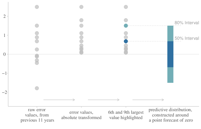
Figure 2: Illustration of the process that we use to construct prediction intervals at the $50\%$ and $80\%$, using forecasts and realized values from the International Monetary Fund World Economic Outlook forecast data.

3.3 Benchmark Models

In order to put the performance of our proposed method in perspective, we compare it to three benchmarks. For the first benchmark (denoted AR), we compute point predictions from an autoregressive model of order one, estimated via ordinary least squares. We fit the model to quarterly data on the predictand (inflation or GDP growth) obtained from the OECD, and construct a forecast of the annual series as a weighted sum of quarterly forecasts. See Section B.1 for details. We then construct prediction intervals from empirical quantiles of the model’s past forecast errors, analogous to our proposed procedure for the IMF forecasts.
For the second benchmark (denoted BVAR), we consider a Bayesian vector autoregressive model specification proposed by Primiceri (2005) and Del Negro and Primiceri (2015), and implemented in the R package bvarsv (Krüger, 2015). In our main results, we consider two quarterly system variables (inflation and GDP growth) obtained from the OECD. In a robustness check described below, we add an index of financial stress as a third variable. Section B.1 provides details. As for the IMF forecasts (and for the AR model), we then construct prediction intervals from empirical quantiles of the BVAR’s past forecast errors.
For the third benchmark (denoted BVAR-direct), we use the same model specification as BVAR, but compute prediction intervals directly from the model’s forecast distribution. That is, the forecast distribution is based on the model’s parametric assumptions, rather than on the empirical distribution of the model’s past point forecast errors.
In order to roughly match the timing of IMF forecasts, we equip the benchmarks for the spring forecasts with data up until the first quarter, and the benchmarks for the fall forecasts with data up until the third quarter.
The AR and BVAR benchmarks are analogous to our proposed methodology (based on IMF forecasts), except that they use a different point forecast. Hence they allow to assess the competitiveness of the IMF’s point forecasts. While AR is simple and transparent, BVAR is much more flexible, allowing for time-varying parameters. The latter comes at the cost of increased complexity (in particular, choice of prior parameters and simulation of the posterior distribution based estimation via Markov chain Monte Carlo methods). In contrast to AR and BVAR, BVAR-direct is fully based on parametric modeling assumptions.

3.4 Forecast Performance on the Hold-Out Data

Here we use the 2013-2023 hold-out data for evaluating the model configuration ($R=11$, absolute error method) chosen as described above. As noted in Section 3.1, we use the first fall release for defining the truth value against which we evaluate the predictions. Figure 3 shows interval scores, whereas Figure 4 shows empirical coverage of the intervals.
For inflation, IMF-based forecasts tend to perform best at the shortest horizon (fall, current year), whereas scores are otherwise similar for all models. The decomposition into the score components is also similar, with dispersion accounting for a sizeable portion of the penalties. Empirical coverage values tend to stay close to nominal levels, for all methods.
For GDP growth, the IMF-based forecasts tend to receive better interval scores than competing methods, across all horizons. The score decomposition is similar for next-year forecasts across methods, with overprediction making up the largest portion, followed by dispersion. Recall that the over- and underprediction components scale linearly with the distance of forecast interval and realized value. Thereby, years such as 2020 with pronounced negative growth rates, which generally were not anticipated a year or more in advance, enter particularly heavily into the overprediction component. Concerning calibration, all methods attain close to nominal empirical coverage levels. The IMF-extracted forecasts overall show little variability in empirical coverage across horizons and countries, but are slightly less well calibrated at the $50\%$ level than competing methods.
All in all, we conclude that IMF-extracted forecasts attain similar or sometimes slightly better performance than competing methods, for both targets and main evaluation metrics used.
Figure 5 shows the average length of the prediction intervals of IMF-extracted probabilistic forecasts, separately for each combination of target variable and forecast horizon. For both inflation and real GDP growth, lengths shrink considerably between next-year and same-year horizons, as well as between the two same-year horizons. The reduction in size is less considerable between the two next-year horizons, especially for inflation, suggesting that the average level of confidence stays mostly similar from one-and-a-half years to one year out from the target. This result is in accordance with Qu et al. (2019), who find no significant evidence that the WEO’s average forecast accuracy improves during this time period.

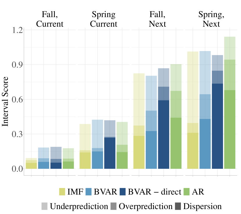
(a) Inflation

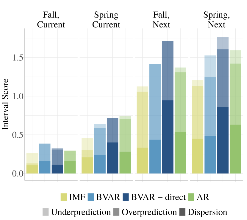
(b) Real GDP growth

Figure 3: Interval scores (IS), separately for (a) inflation and (b) real GDP growth, evaluation period 2013-2023. The IS is decomposed into overprediction, underprediction and dispersion, as indicated by the shaded areas. Scores are computed as a weighted average of individual scores at the $50\%$ and $80\%$ level.

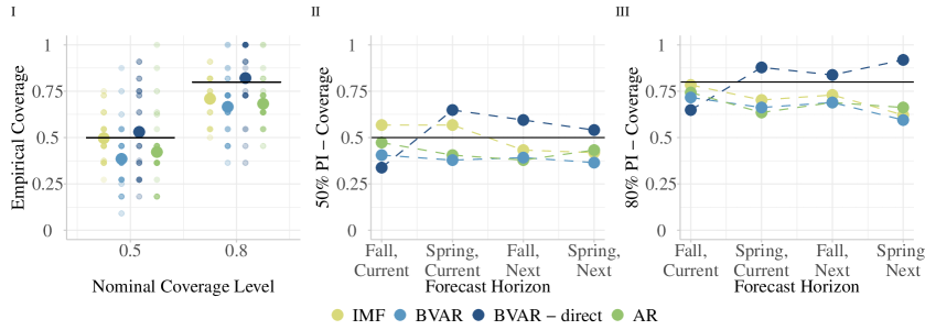
(a) Inflation

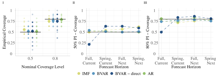
(b) Real GDP growth

Figure 4: Empirical prediction interval coverage levels, for (a) inflation and (b) real GDP growth, evaluation period 2013-2023. In each panel, (I) shows the overall empirical coverage for all methods, with translucent smaller points in the background representing individual coverage for each country-horizon pair, indicating underlying variability in coverage levels. (II) and (III) show coverage levels by forecast horizon, for 50% and 80% nominal coverage, respectively.

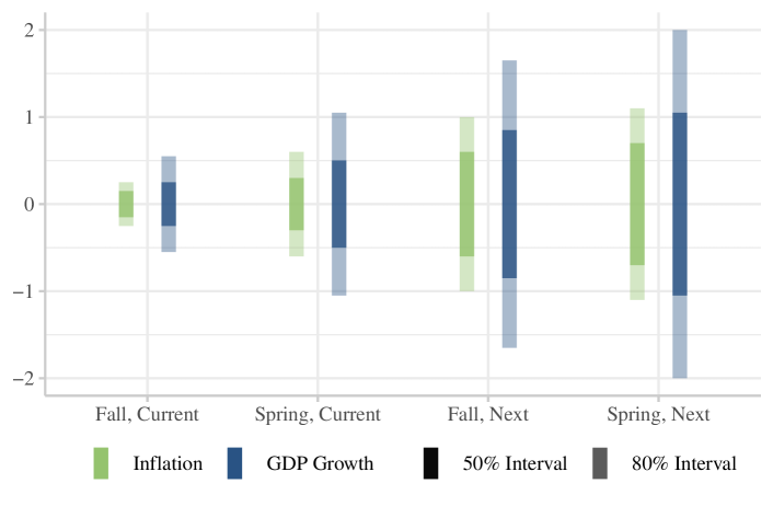
Figure 5: Average length of prediction intervals for IMF-extracted probabilistic forecasts, in the years 2013-2023.

3.5 Robustness Checks

Here we describe two robustness checks on potentially important implementation choices of our empirical setup.

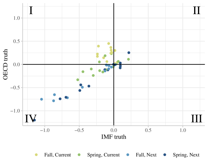
Figure 7: Difference in interval scores (IS) of IMF-extracted and BVAR - direct forecasts $\text{IS}(\text{IMF})-\text{IS}(\text{BVAR-direct})$, when using competing truth values as outcome data. Score differences from using IMF truth values are shown on the x axis, analogously for OECD truth values on the y-axis. Each data point corresponds to one combination of horizon, target variable, and country. Values in quadrants “II” and “IV” represent agreement between the two truth sources on which forecasts are better. Values in quadrant “I” represent instances where the IMF truth prefers the IMF forecasts, but the OECD truth prefers the BVAR forecasts. Values in quadrant “I” represent instances where the IMF truth prefers the BVAR forecasts, but the OECD truth prefers the IMF forecasts.

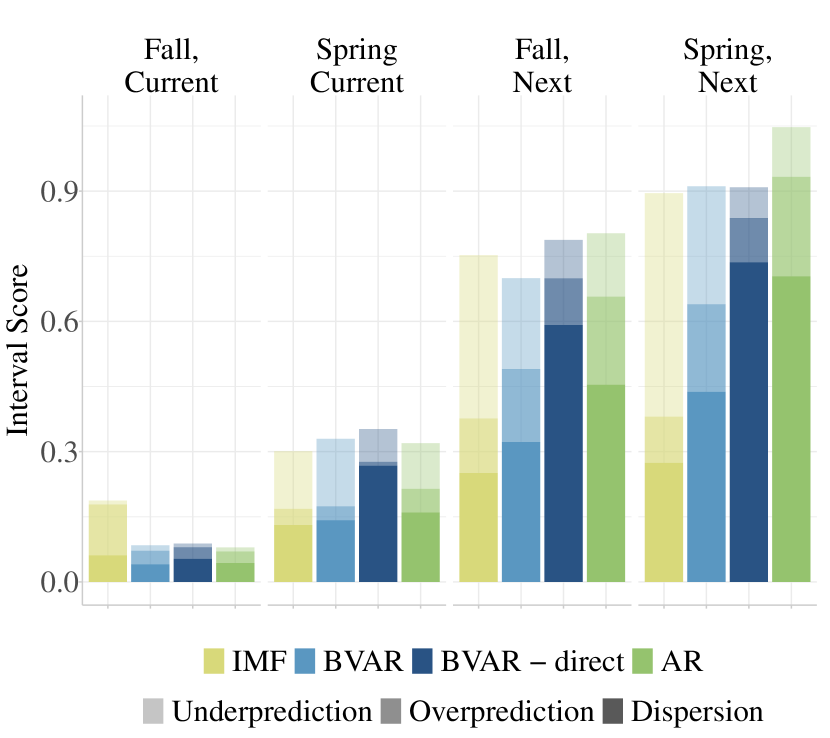
(a) Inflation

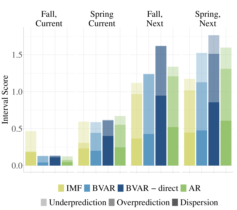
(b) Real GDP growth

Figure 8: Same as Figure 3, but using OECD truth values as the outcome data.

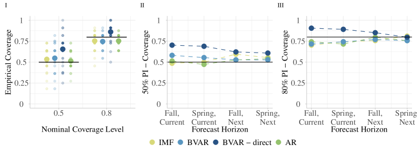
(b) Real GDP growth

Figure 9: Same as Figure 4, but using OECD truth values as the outcome data.

First, we note that the results in Figures 3 and 4 are based on annual truth values provided by the IMF. By contrast, the benchmark models described in Section 3.3 are fitted to higher-frequency (quarterly) data that are not provided by the IMF, and were thus chosen from another source (OECD). While we made our best effort to choose compatible series, full consistency between the two sources seems unrealistic given the complexity of international macroeconomic aggregates. As a consequence, our use of IMF data for evaluation may pose an unfair disadvantage to the benchmark models that were fitted on OECD data. To examine this possibility, we consider an alternative set of annual truth data that we construct from quarterly OECD data. We use these truth data for both the calculation of forecast errors and the subsequent evaluation. Figure 7 in the appendix studies how this change affects interval scores. The figure focuses on the comparison between the IMF-based forecasts and BVAR-direct as an illustrative benchmark method. In a majority of setups (countries, variables and horizons), the different choice of truth value does not change the model ranking between the IMF and BVAR-direct. However, for the shortest horizon (fall, current year), the model ranking is typically reversed in favor of the BVAR-direct method. These results are confirmed by Figures 8 and 9 in the appendix. Thus, while the IMF-based forecasts remain competitive at the other forecast horizons, their good performance at the shortest horizon vanishes when using OECD rather than IMF truth values. While somewhat unsatisfactory, this finding is plausible from a statistical perspective: The shortest forecast horizon is characterized by fairly high predictability since relevant components of the predictand (e.g., GDP growth in 2022) are known when the forecast is issued (e.g., September 2022). In this low-noise setting, the details of the definition of the truth value matter. Hence the IMF-based model outperforms the benchmarks when evaluated against IMF data, whereas the benchmarks prevail when evaluated against OECD data. This effect is not present at longer forecast horizons, where predictability is much lower, so that differences in the definition of the truth value are dominated by other sources of forecast error.

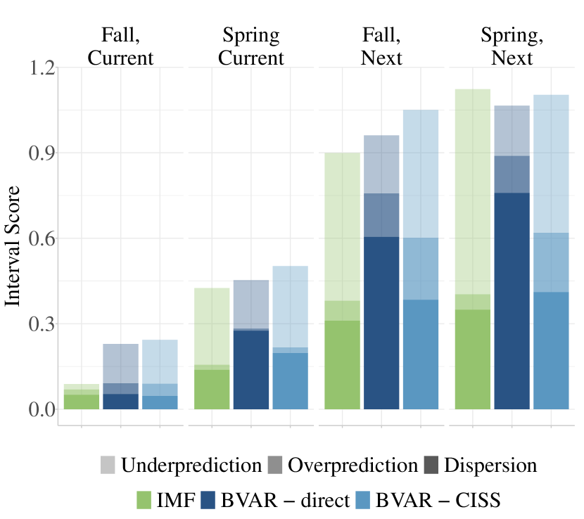
(a) Inflation

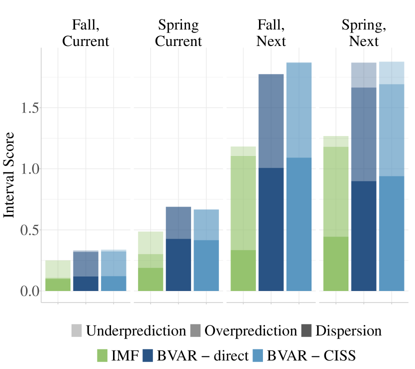
(b) Real GDP growth

Figure 10: Same setup as Figure 3, but with the two BVAR specifications. ‘BVAR-direct’ is the same method as in Figure 3, whereas ‘BVAR-CISS’ additionally includes data from the CISS financial stability index. Here we exclude Japan and Canada from scoring, as we lack predictions from the BVAR - CISS model for these countries.

Second, following Adrian et al. (2019), a recent strand of literature discusses the role of financial stress indexes for predicting inflation and GDP growth. To relate to this discussion, we consider augmenting the BVAR benchmark models by the CISS summary indicator of financial stress (Holló et al., 2012). As shown by Figure 10 in the appendix, the BVAR variant including CISS does not systematically outperform the variant without CISS, in terms of interval scores. Thus, our finding that the IMF-based prediction intervals perform competitively remains intact when augmenting the BVAR benchmarks by information on financial stress.

3.6 Outlook: Prospective Real-Time Forecasts and Evaluation

In addition to the analysis presented so far, we plan to employ the same method in real time and make the resulting probabilistic forecasts publicly available. This is motivated by a lack of easily available probabilistic forecasts for some G7 countries, as discussed in the introduction.
Initial releases of the forecasts for October 2023 and April 2024 are available in a public GitHub repository (Becker et al., 2023), ensuring transparency and accountability through time stamps. The latter repository also links to the website https://probability-forecasting.shinyapps.io/macropi/ on which we provide concise visualizations of all forecasts and prediction intervals. Moreover, we plan to deposit a preregistration protocol (Becker et al., 2023) in which we make a commitment regarding how we will evaluate forecasts in 2029, after collecting five years of prospective forecasts and prediction intervals.

4 Conclusion

This paper presents a method for predicting the distribution of output growth and inflation in the G7 economies. Our method aims to be as simple as possible, subject to being ‘reasonably competitive’, in the sense that we see no straightforward way to improving empirical forecasting performance. While we use point forecasts from the IMF, our suggested procedure can in principle be employed for point forecasts from any source, including macroeconomic model-based forecasts, judgmental forecasts (issued, e.g., by central banks and surveys) or forecasts based on statistical or machine learning models, possibly using a large number of input variables. As an important (and often critical) practical requirement, an informative history of out-of-sample forecast errors must be available in order to estimate the distribution of forecast errors. Our positive empirical results on the IMF forecasts display the common finding that point forecasts by economic institutions are not easy to beat by means of purely statistical models (see e.g. Faust and Wright, 2013).

Appendix

Appendix A Uncertainty Quantification in Central Bank Reports

Protocol for extracting information about uncertainty quantification

We are searching for concretely quantified statements about the uncertainty surrounding macro-economic forecasts in the G7’s central banks’ “flagship” reports for communicating their growth and inflation projections. For this, we applied the following protocol.
We note that this protocol does not necessarily provide a comprehensive view about central banks’ handling of uncertainty quantification and that each central bank might issue explicitly quantified statements about the uncertainty surrounding their macroeconomic forecasts elsewhere. The protocol thus only provides a snapshot view of whether and how central banks communicate uncertainty in their “flagship” reports for macroeconomic projections.

1. Selection of Document.
   For each country, we searched (via the Google search engine) for “[the respective central bank]” + “Macroeconomic Projections”. Subsequently, we selected the first pdf document that stemmed from that central bank and contained forecasts for both GDP growth and inflation. Often, this document would carry the name “Macroeconomic Projections”, alternatively usually ”Monetary Policy Report” or “Economic Outlook”.

2. Information extraction given document

   1. Information around forecasts
      Via a combination of manual and automated search, we navigated to the place in the document that contained macroeconomic forecasts for GDP growth and inflation. These would typically be communicated in a graphical and/or table format. For each graph or table, we checked whether any information additional to a forecast of central tendency was supplied. We also checked the directly surrounding text.

   2. Searching for key terms
      To avoid missing any additional information concerning uncertainty around the communicated forecasts, we additionally searched the document for the following key terms:

      • uncertainty

      • confidence (bands)

      • quantile

      • mean

      • median

      • probabilistic

      • range

      • interval

      Given a match, we determined from context whether the given statement contained any uncertainty quantification for the macroeconomic forecasts in the document.

Country	Name of Central Bank	Name of Document	Edition	UQ present	Form of UQ
Canada	Bank of Canada	Monetary Policy Report	April 2024	no	-
France	Banque de France	Macroeconomic Projections France	September 2023	no	-
Germany	Deutsche Bundesbank	Monthly Report	December 2023	no	-
Italy	Banca d’Italia	Macroeconomic Projections for the Italian economy	April 2024	no	-
Japan	Bank of Japan	Outlook for Economic Activity and Prices	January 2024	somewhat	truncated range of board members’ votes
United Kingdom	Bank of England	Monetary Policy Report	February 2024	yes	fan chart
United States	Federal Reserve	Monetary Policy Report	April 2024	yes	fan chart

Table 3: State of uncertainty quantification for macroeconomic forecasts that are issued by the central banks of the G7 countries. For each central bank, we consulted the “flagship” report containing forecasts for inflation and real GDP growth, often titled “Macroeconomic Projections”, “Economic Outlook” or “Monetary Policy Report” (depending on availability) and checked whether that document’s centrally communicated forecasts are accompanied by an explicit quantification of uncertainty.
¹The latest available report as of Mid April 2024.
²Not all monthly reports contain macroeconomic forecasts - the most recent publication containing them was thus chosen.
³These can’t be interpreted as quantiles of the forecast distribution, as every board member is presumably forecasting a central functional (mean, median, etc.) of the forecast distribution.

Appendix B Details on Empirical Results

B.1 Data for Benchmark Models

CPI: quarterly index data downloaded from https://stats.oecd.org on March 18, 2024; OECD identifier: CPALTT01. We compute inflation rates as logarithmic growth rates of the CPI levels provided by the raw data.
GPD: quarterly growth rates of real GDP downloaded from https://data-explorer.oecd.org/ on March 21; OECD identifier: Table 0102.
CISS: daily values of the CISS index downloaded from https://data.ecb.europa.eu/ on March 18, 2024; series identifier: CISS.D.[country code].Z0Z.4F.EC.SS_CIN.IDX, where country code is a country code (DE = Germany, FR = France, GB = Great Britain, IT = Italy, US = United States of America). We compute quarterly levels of the CISS index by averaging all daily levels within the quarter.
For evaluating forecasts of CPI and GDP, we obtain annual observations as a weighted sum of seven quarterly growth rates, as detailed e.g. in Patton and Timmermann (2011) or Section A.2 of the online supplement for Krüger and Plett (2024). We also use this representation to compute BVAR forecast distributions of the annual predictands, based on the quarterly data to which the BVAR models are fitted.

B.2 Training Sample Performance

			Interval Score			50% Cvg.			80% Cvg.
	Horizon		absolute	directional		absolute	directional		absolute	directional
GDP Growth	Fall, Current		0.23	0.24		0.49	0.43		0.76	0.65
	Spring, Current		0.41	0.41		0.56	0.54		0.76	0.67
	Fall, Next		0.91	0.88		0.49	0.42		0.73	0.70
	Spring, Next		1.14	1.15		0.50	0.40		0.64	0.55
Inflation	Fall, Current		0.12	0.12		0.52	0.44		0.76	0.64
	Spring, Current		0.26	0.25		0.43	0.39		0.75	0.65
	Fall, Next		0.47	0.50		0.40	0.31		0.67	0.54
	Spring, Next		0.52	0.55		0.42	0.38		0.67	0.54

Table 4: Interval scores and interval coverage rates in the training sample (2001-2012), for the directional and the absolute error extraction method. In each block, that is, separately for each combination of target series, horizon, and evaluation metric, the better performing method is highlighted, .

B.3 Choice of Truth Source

(a) Inflation

B.4 Including a Financial Stability Index into the BVAR Benchmark

References

- Adams et al. (2021) Adams, P. A., T. Adrian, N. Boyarchenko, and D. Giannone (2021): “Forecasting macroeconomic risks,” International Journal of Forecasting, 37, 1173–1191.
- Adrian et al. (2019) Adrian, T., N. Boyarchenko, and D. Giannone (2019): “Vulnerable growth,” American Economic Review, 109, 1263–1289.
- Angelopoulos et al. (2023) Angelopoulos, A. N., S. Bates, et al. (2023): “Conformal prediction: A gentle introduction,” Foundations and Trends® in Machine Learning, 16, 494–591.
- Becker et al. (2023) Becker, F., F. Krüger, and M. Schienle (2023): “Macroeconomic prediction intervals - GitHub repository,” Available at https://github.com/KITmetricslab/MacroPI/.
- Bowles et al. (2007) Bowles, C., R. Friz, V. Genre, G. Kenny, A. Meyler, and T. Rautanen (2007): “The ECB Survey of Professional Forecasters (SPF)- A review after eight years’ experience,” ECB Occasional Paper no. 59.
- Bracher et al. (2021a) Bracher, J., E. L. Ray, T. Gneiting, and N. G. Reich (2021a): “Evaluating epidemic forecasts in an interval format,” PLOS Computational Biology, 17, 1–15.
- Bracher et al. (2021b) Bracher, J., D. Wolffram, J. Deuschel, K. Görgen, J. L. Ketterer, A. Ullrich, S. Abbott, M. V. Barbarossa, D. Bertsimas, S. Bhatia, et al. (2021b): “A pre-registered short-term forecasting study of COVID-19 in Germany and Poland during the second wave,” Nature Communications, 12, 5173.
- Breth (1982) Breth, M. (1982): “Nonparametric estimation for a symmetric distribution,” Biometrika, 69, 625–634.
- Clark et al. (2024) Clark, T. E., F. Huber, G. Koop, M. Marcellino, and M. Pfarrhofer (2024): “Investigating Growth-at-Risk using a multicountry non-parametric quantile factor model,” Journal of Business & Economic Statistics, forthcoming.
- Clements (2010) Clements, M. P. (2010): “Explanations of the inconsistencies in survey respondents’ forecasts,” European Economic Review, 54, 536–549.
- Conrad and Enders (2024) Conrad, C. and Z. Enders (2024): “The limits of the ECB’s inflation projections,” SUERF policy brief, No 945.
- Cramer et al. (2022) Cramer, E. Y., E. L. Ray, V. K. Lopez, J. Bracher, A. Brennen, A. J. Castro Rivadeneira, A. Gerding, T. Gneiting, K. H. House, Y. Huang, et al. (2022): “Evaluation of individual and ensemble probabilistic forecasts of COVID-19 mortality in the United States,” Proceedings of the National Academy of Sciences, 119, e2113561119.
- Croushore and Stark (2019) Croushore, D. and T. Stark (2019): “Fifty years of the Survey of Professional Forecasters,” Economic Insights, 4, 1–11.
- de Leeuw et al. (2009) de Leeuw, J., K. Hornik, and P. Mair (2009): “Isotone optimization in R: Pool-adjacent-violators algorithm (PAVA) and active set methods,” Journal of Statistical Software, 32, 1–24.
- Del Negro and Primiceri (2015) Del Negro, M. and G. E. Primiceri (2015): “Time varying structural vector autoregressions and monetary policy: A corrigendum,” The Review of Economic Studies, 82, 1342–1345.
- Elder et al. (2005) Elder, R., G. Kapetanios, T. Taylor, and T. Yates (2005): “Assessing the MPC’s fan charts,” Bank of England Quarterly Bulletin, Autumn, 326–348.
- Elliott et al. (2005) Elliott, G., A. Timmermann, and I. Komunjer (2005): “Estimation and testing of forecast rationality under flexible loss,” The Review of Economic Studies, 72, 1107–1125.
- Faust and Wright (2013) Faust, J. and J. H. Wright (2013): “Forecasting Inflation,” in Handbook of Economic Forecasting, ed. by G. Elliott and A. Timmermann, Elsevier, vol. 2, 2–56.
- Federal Reserve Bank of New York (2024) Federal Reserve Bank of New York (2024): “Outlook-at-Risk: Real GDP growth, unemployment, and inflation,” Available at https://www.newyorkfed.org/research/policy/outlook-at-risk, accessed on February 25, 2024.
- Ganics et al. (2022) Ganics, G., E. Mertens, and T. E. Clark (2022): “What is the predictive value of SPF point and density forecasts?” Federal Reserve Bank of Cleveland, Working Paper No. 22-37.
- Glas and Hartmann (2022) Glas, A. and M. Hartmann (2022): “Uncertainty measures from partially rounded probabilistic forecast surveys,” Quantitative Economics, 13, 979–1022.
- Gneiting et al. (2007) Gneiting, T., F. Balabdaoui, and A. E. Raftery (2007): “Probabilistic forecasts, calibration and sharpness,” Journal of the Royal Statistical Society Series B: Statistical Methodology, 69, 243–268.
- Gneiting and Raftery (2007) Gneiting, T. and A. E. Raftery (2007): “Strictly proper scoring rules, prediction, and estimation,” Journal of the American statistical Association, 102, 359–378.
- Gneiting et al. (2005) Gneiting, T., A. E. Raftery, A. H. Westveld, and T. Goldman (2005): “Calibrated probabilistic forecasting using ensemble model output statistics and minimum CRPS estimation,” Monthly Weather Review, 133, 1098–1118.
- Holló et al. (2012) Holló, D., M. Kremer, and M. Lo Duca (2012): “CISS-a composite indicator of systemic stress in the financial system,” ECB Working paper No. 1426.
- Hyndman and Fan (1996) Hyndman, R. J. and Y. Fan (1996): “Sample quantiles in statistical packages,” The American Statistician, 50, 361–365.
- Inoue et al. (2017) Inoue, A., L. Jin, and B. Rossi (2017): “Rolling window selection for out-of-sample forecasting with time-varying parameters,” Journal of Econometrics, 196, 55–67.
- International Monetary Fund (2024) International Monetary Fund (2024): “World Economic Outlook Database,” Data retrieved from International Monetary Fund. Downloaded via code available at https://github.com/fredbec/imfpp, using direct download link https://www.imf.org/-/media/Files/Publications/WEO/WEO-Database/WEOhistorical.ashx.
- Knüppel et al. (2023) Knüppel, M., F. Krüger, and M.-O. Pohle (2023): “Score-based calibration testing for multivariate forecast distributions,” Preprint, arXiv:2211.16362.
- Krüger (2015) Krüger, F. (2015): bvarsv: Bayesian Analysis of a Vector Autoregressive Model with Stochastic Volatility and Time-Varying Parameters, R package version 1.1.
- Krüger (2017) Krüger, F. (2017): “Survey-based forecast distributions for euro area growth and inflation: Ensembles versus histograms,” Empirical Economics, 53, 235–246.
- Krüger and Plett (2024) Krüger, F. and H. Plett (2024): “Prediction intervals for economic fixed-event forecasts,” Annals of Applied Statistics, 18, 2635–2655.
- Lenza and Primiceri (2022) Lenza, M. and G. E. Primiceri (2022): “How to estimate a vector autoregression after March 2020,” Journal of Applied Econometrics, 37, 688–699.
- Manski (2018) Manski, C. F. (2018): “Survey measurement of probabilistic macroeconomic expectations: progress and promise,” NBER Macroeconomics Annual, 32, 411–471.
- Mass et al. (2009) Mass, C., S. Joslyn, J. Pyle, P. Tewson, T. Gneiting, A. Raftery, J. Baars, J. M. Sloughter, D. Jones, and C. Fraley (2009): “PROBCAST: A web-based portal to mesoscale probabilistic forecasts,” Bulletin of the American Meteorological Society, 90, 1009 – 1014.
- Patton and Timmermann (2011) Patton, A. J. and A. Timmermann (2011): “Predictability of output growth and inflation: A multi-horizon survey approach,” Journal of Business & Economic Statistics, 29, 397–410.
- Pavlova (2024) Pavlova, L. (2024): “Framing effects in consumer expectations surveys,” ZEW Discussion Papers No. 24-036.
- Primiceri (2005) Primiceri, G. E. (2005): “Time varying structural vector autoregressions and monetary policy,” The Review of Economic Studies, 72, 821–852.
- Qu et al. (2019) Qu, R., A. Timmermann, and Y. Zhu (2019): “Do any economists have superior forecasting skills?” Working paper, available at https://dx.doi.org/10.2139/ssrn.3479463.
- Qu et al. (2024) ——— (2024): “Comparing forecasting performance with panel data,” International Journal of Forecasting, 40, 918–941.
- R Core Team (2023) R Core Team (2023): R: A Language and Environment for Statistical Computing, R Foundation for Statistical Computing, Vienna, Austria.
- Raftery (2016) Raftery, A. E. (2016): “Use and communication of probabilistic forecasts,” Statistical Analysis and Data Mining, 9, 397–410.
- Reifschneider and Tulip (2019) Reifschneider, D. and P. Tulip (2019): “Gauging the uncertainty of the economic outlook using historical forecasting errors: The Federal Reserve’s approach,” International Journal of Forecasting, 35, 1564–1582.
- Schick (2024) Schick, M. (2024): “Real-time Nowcasting Growth-at-Risk using the Survey of Professional Forecasters,” Working paper, available at https://dx.doi.org/10.2139/ssrn.4859937.
- Timmermann (2007) Timmermann, A. (2007): “An evaluation of the World Economic Outlook forecasts,” IMF Staff Papers, 54, 1–33.
- Walz et al. (2024) Walz, E.-M., A. Henzi, J. Ziegel, and T. Gneiting (2024): “Easy uncertainty quantification (EasyUQ): Generating predictive distributions from single-valued model output,” SIAM Review, 66, 91–122.
- Winkler (1996) Winkler, R. L. (1996): “Scoring rules and the evaluation of probabilities,” Test, 5, 1–26.