Aliasing and Label-Independent Decomposition of Risk: Beyond the bias–variance trade-off

Abstract

A central problem in data science is to use potentially noisy samples of an unknown function to predict function values for unseen inputs. In classical statistics, the predictive error is understood as a trade-off between the bias and the variance that balances model simplicity with its ability to fit complex functions. However, over-parameterized models exhibit counter-intuitive behaviors, such as “double descent” in which models of increasing complexity exhibit decreasing generalization error. We introduce an alternative paradigm called the generalized aliasing decomposition. We explain the asymptotically small error of complex models as a systematic “de-aliasing” that occurs in the over-parameterized regime. In the limit of large models, the contribution due to aliasing vanishes, leaving an expression for the asymptotic total error we call the invertibility failure of very large models on few training points. Because the generalized aliasing decomposition can be explicitly calculated from the relationship between model class and samples without seeing any data labels, it can answer questions related to experimental design and model selection before collecting data or performing experiments. We demonstrate this approach using several examples, including classical regression problems and a cluster expansion model used in materials science.

Predictive models allow scientists and engineers to extend data and anticipate outcomes for unseen cases. A key issue for these models is the problem of how to understand and minimize generalization error. Traditionally, people thought about generalization error in terms of a trade-off between bias and variance, but that trade-off does not adequately explain the error curves for many models, especially models with more parameters than data points but also highly structured scientific and engineering data. In this work, we introduce a new decomposition, generalized aliasing decomposition, that explains a wide variety of error curves in predictive models for both small (classical) models and for large, overparametrized models. This decomposition explains complex generalization curves, including double and multiple descent, without referencing data labels.

I Introduction

Simple models are generally preferred for many reasons, including interpretability and computational expense [1, 2, 3, 4, 5, 6, 7], but one of the more important justifications for parsimony is a need to balance over- and under-fitting. Models with few parameters avoid making wild predictions but coarsely interpolate the observed data without much fidelity (high bias), while over-parameterized models fit the sampled data well with wild swings in between data points (high variance). The unquestioned goal has been to find the “sweet spot” of model complexity that balances bias and variance, i.e., a faithful model of marginal complexity (see Figure 1, left panel).

While the foregoing story has long been the central dogma of statistics, we now know this view of the fitting problem is not the whole story (see [8] for the bias-variance decomposition for neural networks and [9] for a more thorough presentation of the topic). For extremely over-parameterized models (i.e., more parameters than samples), prediction errors often actually decrease with additional parameters. This phenomenon was recently coined “double descent”[9], although aspects of the phenomena had been known much earlier [10]. More generally, prediction errors may exhibit complex, “multiple descents” [11, 12, 13, 14, 15, 16, 17, 18].

Nonconvex risk curves are most famously recognized in neural networks[19, 20], though this behavior has been observed in various other settings as well (see [10] for a thorough review). Several recent attempts have been made to explain this behavior, focusing on regression and the simplest case of “double descent”, although recent studies show that risk curves may be far more complicated [11]. In [14, 17], the bias–variance decomposition is expanded to explain this non-convex behavior, relying on the interplay between the model design and the actual data. Several other efforts have been made to clarify the relationship between the model class, inherent algorithmic bias, testing and training data, and the appearance of nonmonotonic loss and generalization curves. We do not present a comprehensive summary, but direct the interested reader to [21, 13, 12, 18] that clarify the nature of double descent and its apparent reliance on the structure of the testing and training data sets.

In contrast to these approaches, we build on insights from signal processing [20] and introduce a novel decomposition (34), which we refer to as the generalized aliasing decomposition summarized in the right panel of Figure 1.

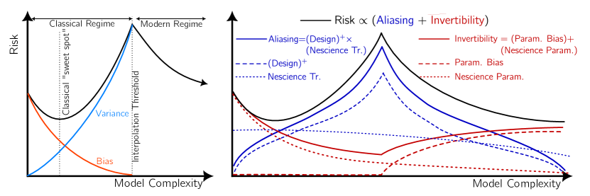
Figure 1: (Left panel) Generalization errors are traditionally understood in terms of the bias–variance trade-off which are difficult to predict in the modern “interpolating” regime. (Right panel) The Generalized Aliasing Decomposition explains generalization curves as contributions from Aliasing (blue) and Invertibility (red). The former explains the structure of mid-sized models, while the latter explains the error for both very small and very large models. Aliasing is further decomposed as contributions coming from the (pseudo) inverse of the traditional design matrix (dashed blue) that account for nonmonotonic structure in the generalization curve and a monotonically decreasing nescience transform that accounts for the scale. The invertibility error is further decomposed in terms of a monotonically increasing parameter bias and monotonically deceasing contributions from nescient parameters. This intuitive, interpretable decomposition applies throughout both classical and modern regimes.

Using this decomposition, we demonstrate that a nonconvex generalization curve is a generic phenomenon, which includes, as a special case, aliasing in the Fourier representation of a time series wherein high-frequency (noisy) components of a signal alias with the lower-frequency (modeled) components, corrupting the representation. Aliasing errors can often be reduced by including more terms in the model class than are required simply from the dimensionality of the data.

The aliasing error is decomposed as the product of the inverse of the classical design matrix and a term we call the nescience transform. The contribution from the design matrix explains much of the nonmonotonic behavior of the generalization curve. Model error due to aliasing increases when the most recently added model terms are linearly dependent on already fitted aspects of the model in the sampled subspace. While this aliasing error is generally maximized at the interpolation threshold, leading to the simplest version of double descent, it is not necessarily maximized there, and real-world sampling strategies can produce complex but understandable error curves (see Figure 4, for example). The scale of the aliasing errors is determined by the norm of the nescience transform. Finally, the asymptotic error is determined by an invertibility term, which can be further decomposed as a sum of bias in the modeled parameters and contributions from the nescient parameters.

Taken collectively, this decomposition explains all the qualitative features of generic risk curves. It further clarifies the roles of model structure, data sampling, data labels, and the learning algorithm in a way that is intuitive while formally facilitating key modeling decisions such as the choice of model class, experimental design, regularization, and learning algorithm.

I.1 Aliasing and Decomposing Risk

To provide a common vocabulary, we start with the familiar example of fitting one-dimensional data to a polynomial. The example illustrates a phenomenon we call the label-independent decomposition of risk and shows that double descent and nonconvex behavior of the generalization curve is a general behavior in fitting problems.

In regression, data $\bm{y}$ are given at samples of an independent variable $t$ and usually decomposed as the sum of an unknown signal $f_{\bm{\theta}}(t)$ parameterized by $\bm{\theta}$ and noise $\xi$:

$$y_{i} =f_{\bm{\theta}}(t_{i})+\xi_{i},$$ (1)

where the subscript $i$ refers to particular data sample. For linear regression the signal is a linear combination of basis functions $f(t)=\sum_{j}\Phi_{j}(t)\theta_{j}$, so that the fundamental regression equation (1) becomes

$$\bm{y} =\mathbf{M}\bm{\theta}+\xi,$$ (2)

where the design matrix $\mathbf{M}$ is composed of samples of basis functions, $\mathbf{M}_{ij}=\Phi_{j}(t_{i})$.

As an illustration, consider a polynomial fit on an interval $[a,b]$, and take the basis functions to be the usual monomial basis $\{1,t,t^{2},t^{3},\dots,t^{d}\}$ for some $d>0$; so $\Phi_{j}=t^{j-1}$, and the design matrix $\mathbf{M}$ is the Vandermonde matrix

$$\mathbf{M}=\begin{pmatrix}1&t_{1}&t_{1}^{2}&\dots&t_{1}^{d}\\ 1&t_{2}&t_{2}^{2}&\dots&t_{2}^{d}\\ \vdots&&&&\vdots\\ 1&t_{n}&t_{n}^{2}&\dots&t_{n}^{d}\end{pmatrix}.$$ (3)

Inferred parameter values $\hat{\bm{\theta}}$ are found by inverting the design matrix. Since $\mathbf{M}$ is generally not square, an appropriate pseudoinverse is used: $\hat{\bm{\theta}}=\mathbf{M}^{+}\bm{y}$. The Moore–Penrose pseudoinverse is the standard choice for linear regression, including this motivating example [23]. Other cases may require an algorithmic solution, but common algorithmic choices, such as stochastic gradient descent, are known to produce similar “norm-minimizing” solutions (see [24, 25, 17], for example).

Finally, predictions at unobserved values of the independent variable are constructed

$$\hat{f}(t)=\sum_{j}\Phi_{j}(t)\hat{\bm{\theta}}_{j}.$$ (4)

A primary quantity of interest is the so-called generalization error or population risk

$$R_{\bm{\theta}}(\hat{f})=\mathbb{E}_{t}[(y(t)-\hat{f}(t))^{2}],$$ (5)

where the expectation $\mathbb{E}$ is taken over a (usually theoretical) distribution of all of the data (not just the training samples), and the dependence of $R_{\bm{\theta}}$ on the model class itself is implicit. A primary goal in data science is to identify the model class and degree of complexity that minimizes risk (5).

II Results

With the context given above in place, we now describe our general results. We first assume that the model functions $\Phi$ may be extended to form a complete set over the space of all possible predictions (including the training points). The Weierstrass approximation theorem [23] guarantees that any continuous function on a closed interval $[a,b]$ can be approximated arbitrarily well by a polynomial; so if the full signal (modeled and unmodeled) is a continuous function, then the infinite monomial basis $\{1,t,t^{2},\dots\}$ is complete, and an appropriate extension for our example.

Because the basis functions $\Phi$ are complete, we can also represent the noise component $\xi$ of the signal as an expansion in $\Phi$. Thus, the fundamental ansatz for our analysis is

$$\bm{y}(t) =f(t)=\sum_{j}\Phi_{j}(t)\theta_{j}.$$ (6)

That is to say, the noisy signal $\bm{y}(t)$ is an abstract vector in a (potentially infinite-dimensional) vector space $\mathcal{D}$ expressed in some basis as

$$\bm{y} =\mathbf{M}\bm{\theta},$$ (7)

where $\mathbf{M}$ is a bounded linear transformation mapping the vector $\bm{\theta}$ in the parameter space $\Theta$ to $\bm{y}$ in the data space $\mathcal{D}$. In the case of fitting a polynomial on an interval $[a,b]$, the operator $\mathbf{M}$ could be thought of as a generalized Vandermonde matrix with countably infinite many rows corresponding to rational points of $[a,b]$ and countably infinitely many columns corresponding to $t^{j}$ for each nonnegative integer $j$.

Performing linear regression on samples of $\bm{y}(t)$ and making predictions at unobserved values of $t$ corresponds to partitioning $\mathcal{D}$ into a direct sum $\mathcal{T}\oplus\mathcal{P}$ of training $\mathcal{T}$ and prediction $\mathcal{P}$ subspaces. We write $\bm{y}$ in this decomposition as $\bm{y}=(\bm{y}_{\mathcal{T}},\bm{y}_{\mathcal{P}})$. We assume that $\mathcal{T}$ has finite dimension $n$, but $\mathcal{P}$ need not be finite-dimensional. The learning problem is this: Given observations in $\bm{y}_{\mathcal{T}}$, predict the components of $\bm{y}_{\mathcal{P}}$. In practice, this is done by similarly partitioning the representation space $\Theta=\mathcal{M}\oplus\mathcal{U}$ into a modeled $\mathcal{M}$ and an unmodeled $\mathcal{U}$ subspace so that $\bm{\theta}=(\bm{\theta}_{\mathcal{M}},\bm{\theta}_{\mathcal{U}})$. With these partitions, the relationship of (7) between data and coordinates takes the block representation described in the definition below.

Definition.

Denote the decomposition of the labeled data as

$$\left(\begin{array}[]{c}\bm{y}_{\mathcal{T}}\\ \bm{y}_{\mathcal{P}}\end{array}\right) =\left(\begin{array}[]{cc}\mathbf{M}_{\mathcal{T}\mathcal{M}}&\mathbf{M}_{\mathcal{T}\mathcal{U}}\\ \mathbf{M}_{\mathcal{P}\mathcal{M}}&\mathbf{M}_{\mathcal{P}\mathcal{U}}\\ \end{array}\right)\left(\begin{array}[]{c}\bm{\theta}_{\mathcal{M}}\\ \bm{\theta}_{\mathcal{U}}\end{array}\right),$$ (14)

where the linear transformation $\mathbf{M}_{\mathcal{T}\mathcal{M}}:\mathbb{R}^{m}\to\mathbb{R}^{n}$ is the usual design matrix and we call the linear transformation $\mathbf{M}_{\mathcal{T}\mathcal{U}}$ the nescience transformation.

We use the word nescience in the definition to emphasize the fact that the unmodeled part of the function $f$ is effectively unknown to us (noise, for example). Because $\mathbf{M}$ is bounded and linear, the subblocks $\mathbf{M}_{\mathcal{T}\mathcal{U}}$, $\mathbf{M}_{\mathcal{P}\mathcal{M}}$, and $\mathbf{M}_{\mathcal{P}\mathcal{U}}$ are also bounded linear transformations.

In the case of fitting a polynomial of degree at most $d$ on $n$ training points $t_{1},\dots t_{n}$, the design matrix (upper left block) $\mathbf{M}_{\mathcal{T}\mathcal{M}}$ is the Vandermonde matrix in  (3) and the nescience transformation (upper right block) is the semi-infinite matrix

$$\mathbf{M}_{\mathcal{T}\mathcal{U}}=\begin{pmatrix}t_{1}^{d+1}&t_{1}^{d+2}&\dots\\ t_{2}^{d+1}&t_{2}^{d+2}&\dots\\ \vdots&\vdots\\ t_{n}^{d+1}&t_{n}^{d+2}&\dots\\ \end{pmatrix}.$$

The rows of the lower blocks correspond to the points in $[a,b]\setminus\{t_{1},\dots,t_{n}\}$. The columns of the lower left block correspond to the monomials $1,t,t^{2},\dots,t^{d}$ (spanning the space $\mathcal{M}$) evaluated at the points of $[a,b]\setminus\{t_{1},\dots,t_{n}\}$. The columns of the lower right block correspond to the unmodeled monomials $t^{d+1},t^{d+2},\dots$ (spanning $\mathcal{U}$), evaluated at points of $[a,b]\setminus\{t_{1},\dots,t_{n}\}$.

We learn the modeled parameters $\hat{\bm{\theta}}_{\mathcal{M}}$ using some pseudoinverse $\mathbf{M}_{\mathcal{T}\mathcal{M}}^{+}$ of the design matrix $\mathbf{M}_{\mathcal{T}\mathcal{M}}$:

$$\hat{\bm{\theta}}_{\mathcal{M}} =\mathbf{M}_{\mathcal{T}\mathcal{M}}^{+}\,\bm{y}_{\mathcal{T}}.$$ (15)

Inferring only $\hat{\bm{\theta}}_{\mathcal{M}}$ is equivalent to assuming that the unmodeled parameters vanish, so $\hat{\bm{\theta}}_{\mathcal{U}}=\bm{0}$ and $\hat{\bm{\theta}}=(\hat{\bm{\theta}}_{\mathcal{M}},\bm{0})$. However, the true representation of the training data $\bm{y}_{\mathcal{T}}$ includes contributions from both the modeled and nescient components of $\bm{\theta}$:

$$\bm{y}_{\mathcal{T}}=\mathbf{M}_{\mathcal{T}\mathcal{M}}\bm{\theta}_{\mathcal{M}}+\mathbf{M}_{\mathcal{T}\mathcal{U}}\bm{\theta}_{\mathcal{U}}.$$

Notice that the nescient term $\mathbf{M}_{\mathcal{T}\mathcal{U}}\bm{\theta}_{\mathcal{U}}$ corresponds to the noise in (1). The inferred parameters $\hat{\bm{\theta}}_{\mathcal{M}}$ are distorted by the nescience term, which, in our extended representation, takes the form:

$$\hat{\bm{\theta}}_{\mathcal{M}} =\left(\mathbf{M}_{\mathcal{T}\mathcal{M}}^{+}\mathbf{M}_{\mathcal{T}\mathcal{M}}\right)\bm{\theta}_{\mathcal{M}}+\left(\mathbf{M}_{\mathcal{T}\mathcal{M}}^{+}\mathbf{M}_{\mathcal{T}\mathcal{U}}\right)\bm{\theta}_{\mathcal{U}}.$$ (16)

For conceptual clarity, we write this as

$$\hat{\bm{\theta}}=\left(\begin{array}[]{c}\hat{\bm{\theta}}_{\mathcal{M}}\\ 0\end{array}\right) =\left(\begin{array}[]{cc}\mathbf{M}_{\mathcal{T}\mathcal{M}}^{+}\mathbf{M}_{\mathcal{T}\mathcal{M}}&\mathbf{M}_{\mathcal{T}\mathcal{M}}^{+}\mathbf{M}_{\mathcal{T}\mathcal{U}}\\ 0&0\end{array}\right)\bm{\theta}$$ (20)

$$=\left(\begin{array}[]{cc}\mathbf{B}&\mathbf{A}\\ 0&0\end{array}\right)\bm{\theta},$$ (23)

where we have defined

$$\mathbf{A}=\mathbf{M}_{\mathcal{T}\mathcal{M}}^{+}\mathbf{M}_{\mathcal{T}\mathcal{U}}\quad\text{ and }\quad\mathbf{B}=\mathbf{M}_{\mathcal{T}\mathcal{M}}^{+}\mathbf{M}_{\mathcal{T}\mathcal{M}},$$ (24)

and $\bm{\theta}$ is the vector of parameters that represents the complete signal precisely.

We call $\mathbf{A}$ the generalized aliasing operator. It quantifies how the effects of the unmodeled, nescient parameters $\bm{\theta}_{\mathcal{U}}$ are redirected into the modeled parameters. Note that $\mathbf{A}$ depends not only on the partition between modeled parameters and unmodeled modes, but also on the partition between training points and prediction points and the choice of pseudoinverse (or the choice of learning algorithm more generally).

In the case of Fourier series, the concept of aliasing refers to the distortion of a low-frequency signal by high-frequency modes. Expressed in the form we have described, Fourier aliasing is found from $\mathbf{A}=\mathbf{M}_{\mathcal{T}\mathcal{M}}^{+}\mathbf{M}_{\mathcal{T}\mathcal{U}}$, expressed in the Fourier basis for uniform samples (see Section II.II.3 for more on aliasing for Fourier series), where it can be expressed in closed-form. More generally, $\mathbf{A}$ quantifies how unmodeled components affect the signal at the sampled points, leading to a misrepresentation of the inferred modeled parameters that we call generalized aliasing.

II.1 Error Decomposition and Analysis

The model described above uses $\hat{\bm{\theta}}=(\hat{\bm{\theta}}_{\mathcal{M}},\bm{0})$ to approximate the true function $\bm{y}$ with the model output:

$$\hat{\bm{y}} =\mathbf{M}\hat{\bm{\theta}}=\mathbf{M}\mathbf{M}_{\mathcal{T}\mathcal{M}}^{+}\bm{y}_{\mathcal{T}}=\mathbf{M}(\mathbf{B}\bm{\theta}_{\mathcal{M}}+\mathbf{A}\bm{\theta}_{\mathcal{U}}).$$ (25)

Comparing this with the true $\bm{y}=\mathbf{M}\bm{\theta}$, we are interested in the risk (5), which, assuming that the points $t$ are drawn from a uniform distribution, is

$$R_{\bm{\theta}}(\hat{\bm{y}}) =\mathbb{E}_{t}[(\bm{y}(t)-\hat{\bm{y}}(t))^{2}]=\sum_{t}(\bm{y}(t)-\hat{\bm{y}}(t))^{2}$$

$$=\|\bm{y}-\hat{\bm{y}}\|^{2}$$ (26)

$$=\left\|\mathbf{M}\begin{pmatrix}\mathbf{I}_{m}-\mathbf{B}&-\mathbf{A}\\ 0&\mathbf{I}\end{pmatrix}\bm{\theta}\right\|^{2},$$ (27)

where the norm $\|\cdot\|$ is the $2$-norm $\|\cdot\|_{2}$. This motivates the definition of the parameter error operator

$$\mathbf{E}_{\bm{\theta}}=\left(\begin{array}[]{cc}\mathbf{I}_{m}-\mathbf{B}&-\mathbf{A}\\ 0&\mathbf{I}\end{array}\right).$$ (30)

We have used the subscript $\bm{\theta}$ to indicate that $\mathbf{E}_{\bm{\theta}}\bm{\theta}$ represents errors in the inferred parameters, rather than the errors $\bm{y}-\hat{\bm{y}}$ in the signal.

II.1.1 Bias and Variance

For a fixed decomposition $\Theta=\mathcal{M}\oplus\mathcal{U}$, the estimator $\hat{\bm{y}}$ and the operators $\mathbf{A}$, $\mathbf{B}$, and $\mathbf{E}_{\bm{\theta}}$ depend on the choice $T=\{t_{1},\dots,t_{n}\}$ of the training points. The expected value $\mathbb{E}_{T}(R_{\bm{\theta}}(\hat{\bm{y}}))=\mathbb{E}_{T}\left[\|\hat{\bm{y}}-\bm{y}\|^{2}\right]$ of the risk (taken over the distribution of $T$) is often decomposed into a sum of a bias term and a variance term; see, for example, [29, §20.1]. In our current setting, this decomposition is not intuitive and is difficult to analyze. We find it much more natural, and easier, to analyze the risk $\|\bm{y}-\hat{\bm{y}}\|^{2}$ and its expected value $\mathbb{E}_{T}\!\left[\|\bm{y}-\hat{\bm{y}}\|^{2}\right]$ directly, rather than to analyze the bias and variance terms separately.

II.1.2 Aliasing and Invertibility Error

A central question is how the risk changes with the dimension $m$ of the modeled space $\mathcal{M}$. Observe that

$$R_{\bm{\theta}}(\hat{\bm{y}})=\|\mathbf{M}\mathbf{E}_{\bm{\theta}}\bm{\theta}\|^{2}\leq\|\mathbf{M}\|^{2}\|\mathbf{E}_{\bm{\theta}}\|^{2}\|\bm{\theta}\|^{2},$$

where the norm on the linear transformations $\mathbf{M}$ and $\mathbf{E}_{\bm{\theta}}$ is the induced norm, defined as

$$\|\mathbf{M}\|=\max_{\|\bm{\theta}\|=1}\|\mathbf{M}\bm{\theta}\|\qquad\text{and}\qquad\|\mathbf{E}\|=\max_{\|\bm{\theta}\|=1}\|\mathbf{E}\bm{\theta}\|.$$

In the finite dimensional case (where the transformations are represented by matrices) it is well known that if the norm on both the domain and range of a matrix is the usual (two-) norm, then the induced norm is its largest singular value. In this case the induced norm is often called the spectral norm.

We assume the transformation $\mathbf{M}$ has a bounded norm and note that its norm is independent of the choice of model $\mathcal{M}$. The overall error certainly depends on $\bm{\theta}$ and its norm, but, as we show below, the non-convex generalization is largely driven by the parameter error operator $\mathbf{E}_{\bm{\theta}}$, rather than by specific choices of $\bm{\theta}$. We focus now on $\mathbf{E}_{\bm{\theta}}$ and write it as a sum of a term proportional to $\mathbf{A}$ and the remainder:

$$\mathbf{E}_{\bm{\theta}} =\left(\begin{array}[]{cc}0&-\mathbf{A}\\ 0&0\end{array}\right)+\left(\begin{array}[]{cc}I-\mathbf{B}&0\\ 0&I\end{array}\right)$$ (34)

$$=\mathbf{E}_{\mathbf{A}}+\mathbf{E}_{\mathbf{B}}$$ (35)

The operator $\mathbf{E}_{\mathbf{A}}$ measures the effect of aliasing, and the operator $\mathbf{E}_{\mathbf{B}}$ essentially measures two things: first, the failure of $\mathbf{M}_{\mathcal{T}\mathcal{M}}$ to be invertible (in the upper-left block), and second, how much of the signal is nescient, i.e., unmodeled (the lower-right identity block). The general shape of these different contributions to the risk is illustrated in the right panel of Figure 1. We now analyze each of $\mathbf{E}_{\mathbf{A}}$ and $\mathbf{E}_{\mathbf{B}}$ in turn.

II.1.3 Analysis of $\|\mathbf{E}_{\mathbf{A}}\|$ and $\|\mathbf{E}_{\mathbf{A}}\,\bm{\theta}\|$

Assuming that $\bm{\theta}$ and $\mathbf{M}$ are fixed with bounded norms, the norm $\|\mathbf{M}_{\mathcal{T}\mathcal{U}}\|$ of the nescience matrix is bounded by the norm of $\mathbf{M}$ and is a nonincreasing function of the model dimension $m$ (see Section IV.IV.2.1 for details), which means that the structure of

$$\|\mathbf{E}_{\mathbf{A}}\bm{\theta}\| =\|\mathbf{A}\bm{\theta}_{\mathcal{U}}\|=\|\mathbf{M}_{\mathcal{T}\mathcal{M}}^{+}\mathbf{M}_{\mathcal{T}\mathcal{U}}\bm{\theta}_{\mathcal{U}}\|$$

$$\leq\|\mathbf{M}_{\mathcal{T}\mathcal{M}}^{+}\|\|\mathbf{M}_{\mathcal{T}\mathcal{U}}\|\|\bm{\theta}_{\mathcal{U}}\|$$

as a function of $m$ is primarily determined by the norm of the inverse design matrix $\mathbf{M}_{\mathcal{T}\mathcal{M}}^{+}$.

Consider the situation where a given decomposition $\Theta=\mathcal{M}\oplus\mathcal{U}$ of parameter space with design matrix $\mathbf{M}_{\mathcal{T}\mathcal{M}}$ and nescience $\mathbf{M}_{\mathcal{T}\mathcal{U}}$ is changed by moving one column $\bm{\varphi}$ out of the nescience matrix and into the design matrix. This always decreases (or rather never increases) the norm $\|\mathbf{M}_{\mathcal{T}\mathcal{U}}\|$ but the effect on $\|\mathbf{M}_{\mathcal{T}\mathcal{M}}^{+}\|$ is determined primarily by whether $\bm{\varphi}$ is linearly independent from the other columns of $\mathbf{M}_{\mathcal{T}\mathcal{M}}$ or not, as described in the following theorem (proved in Section IV.IV.2).

Theorem II.1.

When changing the model by moving one column $\bm{\varphi}$ out of the nescience matrix and into the design matrix, the norm $\|\mathbf{M}_{\mathcal{T}\mathcal{U}}\|$ never increases and

• $\|\mathbf{M}_{\mathcal{T}\mathcal{M}}^{+}\|$ cannot decrease if $\bm{\varphi}$ is linearly independent of the other columns of $\mathbf{M}_{\mathcal{T}\mathcal{M}}$,

• $\|\mathbf{M}_{\mathcal{T}\mathcal{M}}^{+}\|$ cannot increase if $\bm{\varphi}$ is linearly dependent upon the other columns of $\mathbf{M}_{\mathcal{T}\mathcal{M}}$.

Moreover, as the model dimension $m$ increases to $\infty$, the norm $\|\mathbf{M}_{\mathcal{T}\mathcal{M}}^{+}\|$ shrinks to $0$, almost surely.

Although it can be arranged so that $\|\mathbf{M}_{\mathcal{T}\mathcal{M}}^{+}\|$ remains constant when moving one column $\bm{\varphi}$ fom $\mathbf{M}_{\mathcal{T}\mathcal{U}}$ to $\mathbf{M}_{\mathcal{T}\mathcal{M}}$, in most cases we see a significant increase in $\|\mathbf{M}_{\mathcal{T}\mathcal{M}}^{+}\|$ whenever $\bm{\varphi}$ is independent from the previous columns and a significant decrease in $\|\mathbf{M}_{\mathcal{T}\mathcal{M}}^{+}\|$ whenever $\bm{\varphi}$ is dependent upon the previous columns.

Theorem II.1 explains the sharp peaks in generalization curves described as double and multiple descent, and it is relevant to other nonmonotonic features in both the under- and over-parameterized regimes, as we now describe.

For a generic $\mathbf{M}$ the columns are typically arranged so that for $m<n$ each column $\bm{\varphi}_{m+1}$ is independent of the previous columns of $\mathbf{M}_{\mathcal{T}\mathcal{M}}$. Hence, as $m$ increases the norm $\|\mathbf{M}_{\mathcal{T}\mathcal{M}}^{+}\|$ is expected to grow nearly monotonically until the interpolation threshold $m=n$. And once $m\geq n$ the columns of $\mathbf{M}_{\mathcal{T}\mathcal{M}}$ are expected to span the column space of the entire training set $(\mathbf{M}_{\mathcal{T}\mathcal{M}}|\mathbf{M}_{\mathcal{T}\mathcal{U}})$ of the operator $\mathbf{M}$, so each new column added to $\mathbf{M}_{\mathcal{T}\mathcal{M}}$ typically decreases the norm $\|\mathbf{M}_{\mathcal{T}\mathcal{M}}^{+}\|$.

In this case, $\|\mathbf{M}_{\mathcal{T}\mathcal{M}}^{+}\|$ is a nondecreasing function of $m$ until $m=n$, after which it is nonincreasing. The common peak in the generalization error at the interpolation threshold is thus understood as the peak in $\|\mathbf{M}_{\mathcal{T}\mathcal{M}}^{+}\|$ at $m=n$. More complicated generalization curves can be generically understood by considering $\bm{\varphi}_{m+1}$’s linear (in)dependence on the previously modeled terms.

Regardless of the ordering of the columns of $\mathbf{M}$, the upper bound

$$\|\mathbf{A}\|\leq\|\mathbf{M}_{\mathcal{T}\mathcal{M}}^{+}\|\|\mathbf{M}_{\mathcal{T}\mathcal{U}}\|$$

cannot increase when stepping from $m$ to $m+1$ unless the next column $\bm{\varphi}_{m+1}$ is independent of the previous columns. Moreover, the bound will almost surely shrink to $0$ as $m\to\infty$.

Of course, one can arrange to add columns to $\mathbf{M}_{\mathcal{T}\mathcal{M}}$ in a way that the rank of $\mathbf{M}_{\mathcal{T}\mathcal{M}}$ grows slower than expected, permitting the construction of descent curves for $\|\mathbf{A}\|$ of various shapes. But when the columns are sufficiently general (as, for example, with the random ReLU features (RRF) model and the random Fourier features (RFF) model), the result for $\|\mathbf{A}\|$ is similar in shape to the standard double descent curve for mean-squared error, described in [9] with a single large peak at the interpolation threshold and decreasing monotonically thereafter (see Figure 2).

II.1.4 Analysis of $\|\mathbf{E}_{\mathbf{B}}\|$ and $\|\mathbf{E}_{\mathbf{B}}\,\bm{\theta}\|$

It is straightforward (see Section IV.IV.3 for details) to show that $\mathbf{E}_{\mathbf{B}}$ can be written as

$$\mathbf{E}_{\mathbf{B}}=\begin{pmatrix}\mathbf{P}_{\mathcal{N}}&0\\ 0&\mathbf{I}_{\mathcal{U}}\end{pmatrix},$$ (36)

where $\mathbf{P}_{\mathcal{N}}$ is the orthogonal projection of $\mathcal{M}$ onto the null space $\mathcal{N}\subseteq\mathcal{M}$ of $\mathbf{M}_{\mathcal{T}\mathcal{M}}$, and where $\mathbf{I}_{\mathcal{U}}$ is the identity operator on the nescient space $\mathcal{U}$. This implies that its induced operator norm is always equal to $1$, and the norm of the product $\mathbf{E}_{\mathbf{B}}\bm{\theta}$ is bounded by the norm of $\bm{\theta}$:

$$\|\mathbf{E}_{\mathbf{B}}\bm{\theta}\|\leq\|\mathbf{E}_{\mathbf{B}}\|\|\bm{\theta}\|=\|\bm{\theta}\|.$$ (37)

To make more fine-grained statements about the dependence of $\mathbf{E}_{\mathbf{B}}\bm{\theta}$ on the model dimension $m$, we write

$$\|\mathbf{E}_{\mathbf{B}}\bm{\theta}\|^{2}=\|\mathbf{P}_{\mathcal{N}(m)}\bm{\theta}_{\mathcal{M}(m)}\|^{2}+\|\bm{\theta}_{\mathcal{U}(m)}\|^{2}$$ (38)

where we have made the $m$-dependence explicit. Notice that the first term $\|\mathbf{P}_{\mathcal{N}}\bm{\theta}_{\mathcal{M}}\|^{2}=\|\bm{\theta}_{\mathcal{M}}-\hat{\bm{\theta}}_{\mathcal{M}}\|^{2}$ is the (square of the) bias in $\bm{\theta}_{\mathcal{M}}$ while the second term is exclusively from the nescient parameters, $\bm{\theta}_{\mathcal{U}}$. Since $\mathcal{N}(m)\subseteq\mathcal{N}(m+1)$, it follows that the contribution $\|\mathbf{P}_{\mathcal{N}}\bm{\theta}_{\mathcal{M}}\|$ from parameter bias is a nondecreasing function of $m$. In contrast, the contributions from the nescient parameters is nonincreasing, since it decreases by exactly $|\theta_{m+1}|^{2}$ at each step. Depending on the structure of the parameter vector, the full invertibility error may have nonmonotonic behavior due to the interplay between these contributions.

We first introduce the unstructured model ansatz in which components of $\bm{\theta}$ are independent, identically distributed random variables with mean zero and variance $\sigma^{2}$. In this setting the expected invertibility error is

$$\mathbb{E}_{\theta}\left[\|\mathbf{E}_{\mathbf{B}}\bm{\theta}\|^{2}\right] =\sigma^{2}\left(\operatorname{Tr}\mathbf{P}_{\mathcal{N}}+\operatorname{Tr}\mathbf{I}_{\mathcal{U}}\right)$$ (39)

$$=\sigma^{2}(\dim\mathcal{N}+\dim\mathcal{U}).$$ (40)

At each step, $\dim\mathcal{U}$ decreases by one, while $\dim\mathcal{N}$ increases by either zero or one so the total invertibility error is a strictly nonincreasing function of $m$.

In the generic case, $\dim\mathcal{N}(m)=0$ when the number $n$ of rows (data points) is less than the number $m$ of columns (model parameters). This is the well-known fact that the ordinary least squares estimator is unbiased. However, for $m>n$, $\dim\mathcal{N}(m+1)=\dim\mathcal{N}(m)+1$, so parameter bias grows monotonically beyond the interpolation threshold and, on average, cancels the decrease from the nescient parameters.

In contrast to the unstructured case, modelers often have prior information about which parameters are most important and preferentially order the parameter vector to reflect this. In such cases, the total parameter error $\|(\mathbf{E}_{\mathbf{A}}+\mathbf{E}_{\mathbf{B}})\bm{\theta}\|$ tends to be dominated by the invertibility error $\|\mathbf{E}_{\mathbf{B}}\bm{\theta}\|$ for very small and very large model size $m$, where aliasing $\|\mathbf{E}_{\mathbf{A}}\bm{\theta}\|$ is small. For very small $m$, as $m$ increases there is often an initial descent of parameter error due to fewer nescient terms and the model’s increasing ability to capture the signal faithfully. This is conceptually analogous to reducing bias in the classical bias–variance paradigm. However, for very large models, the parameter bias can grow faster than the decrease in the nescient contribution, resulting in growing $\|\mathbf{E}_{\mathbf{B}}\bm{\theta}\|$ as depicted in Fig. 1. This growing error for large models is not analogous to variance and cannot be termed over-fitting. Rather, it reflects the lack of invertibility for large models, specifically, larger parameter bias as more of the mass of $\bm{\theta}$ is projected into the kernel $\mathcal{N}$ of the design matrix $\mathbf{M}_{\mathcal{T}\mathcal{M}}$.

We refer to the phenomenon of nonmonotonic behavior in the invertibility error as over-modeling. Over-modeling is the dominant error in the asymptotic limit of $m\rightarrow\infty$, as contributions from both aliasing and nescience vanish almost surely. The over-modeling phenomenon has largely been overlooked in the double descent literature because it is absent in the unstructured model approach used by most theoretical studies. The example in subsection II.4 below illustrates that unstructured models tend to have optimal performance in the asymptotic limit, while models that exploit prior information often have optimal performance at the classical “sweet spot,” due to asymptotic over-modeling.

II.2 Some Examples

Although the motivating example in Section I.1 for the aliasing decomposition was focused on one-dimensional polynomials, this decomposition applies much more generally to the problem of fitting a function $f:\mathbb{R}^{d}\to\mathbb{R}$ or $f:\mathbb{R}^{d}\to\mathbb{C}$ for arbitrary $d$. We illustrate this with examples of two different choices of models applied to three different data sets. The two bases are random Fourier features (RFF) and random ReLU features (RRF) (described in [9] and [32]).

All of these basis functions are of the form $\phi_{k}(\bm{t})=\sigma(\langle\bm{t},\bm{v}_{k}\rangle)$, where the $\bm{v}_{k}\in\mathbb{R}^{d}$ are i.i.d. normal, and $\sigma$ is some activation function. In the case of the RRF model, the activation function is the usual ReLU, and in the case of RFF the activation function is $\sigma(x)=\exp(i\pi x)$. The models that result from using these two choices (either RRF or RFF) can both be thought of as 2-layer neural networks of the form

$$y(\bm{t})=\sum_{k=1}^{m}\theta_{k}\phi_{k}(\bm{t})=\sum_{k=1}^{m}\theta_{k}\sigma(\langle\bm{t},\bm{v}_{k}\rangle).$$

The data sets are (unlableled) images from MNIST and CIFAR-10 and points from the Mei–Montanari [32] sphere $\mathbb{S}^{d-1}(\sqrt{d})$, where we have arbitrarily fixed $d=1024$. In each case 1,000 training points $\bm{t}_{i}$ were drawn uniformly and evaluated at 6,000 basis functions (either RRF or RFF). The columns of the resulting design matrix $\mathbf{M}_{\mathcal{T}\mathcal{M}}$ and nescience matrix $\mathbf{M}_{\mathcal{T}\mathcal{U}}$ are all of the form $\bm{\varphi}_{k}=(\phi_{k}(\bm{t}_{1}),\dots,\phi_{k}(\bm{t}_{n}))$.

In Figure 2 we show the norms of the matrices $\mathbf{A}$, $\mathbf{M}_{\mathcal{T}\mathcal{M}}^{+}$, and $\mathbf{M}_{\mathcal{T}\mathcal{U}}$ as functions of the number $m$ of parameters for these models on the three different datasets. The horizontal axis in Figure 2 indicates the number $m$ of parameters, while the vertical axis shows the norm $\|\mathbf{E}_{\mathbf{A}}\|=\|\mathbf{A}\|$ and the norms $\|\mathbf{M}_{\mathcal{T}\mathcal{M}}^{+}\|$ and $\|\mathbf{M}_{\mathcal{T}\mathcal{U}}\|$ of its two factors. The norm $\|\mathbf{M}_{\mathcal{T}\mathcal{U}}\|$ of the nescience matrix is strictly nonincreasing, while the peak at the interpolation threshold $m=n$ comes entirely from the pseudoinverse $\|\mathbf{M}_{\mathcal{T}\mathcal{M}}^{+}\|$ of the design matrix.

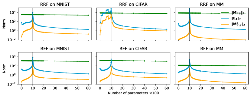
Figure 2: The induced (spectral) norm of the error matrix $\mathbf{E}_{\mathbf{A}}$, and its factors, the design matrix $\mathbf{M}_{\mathcal{T}\mathcal{M}}^{+}$ and nescience matrix $\mathbf{M}_{\mathcal{T}\mathcal{U}}$ for the random Fourier features (RFF) model and the random ReLU features (RRF) model on the MNIST and CIFAR-10 datasets, as in [9], as well as on the Mei-Montanari (MM) sphere [32]. In each case the models were trained on 1,000 randomly chosen training points (vertical black line) with the number of modeled parameters ranging from 1 up to 6,000. The norm $\|\mathbf{E}_{\mathbf{A}}\|$ is bounded by the product of $\|\mathbf{M}_{\mathcal{T}\mathcal{M}}^{+}\|$ and $\|\mathbf{M}_{\mathcal{T}\mathcal{U}}\|$. The norm $\|\mathbf{M}_{\mathcal{T}\mathcal{U}}\|$ is nonincreasing and decreases slowly, so the familiar double descent shape with a peak at the interpolation threshold is driven by $\|\mathbf{M}_{\mathcal{T}\mathcal{M}}^{+}\|$.

In the examples in Figure 2 the norm $\|\mathbf{M}_{\mathcal{T}\mathcal{M}}^{+}\|$ generally increases up to the interpolation threshold because the random choices in RRF and RFF make it likely that the first $n$ columns $\bm{\varphi}_{1},\dots,\bm{\varphi}_{n}$ are linearly independent. The norm then decreases after the interpolation threshold because all the subsequent columns are, of necessity, linearly dependent on the columns that precede them.

II.3 Why ‘aliasing’? Discrete Fourier series

To clarify the name “generalized aliasing,” we turn to an example familiar in the signals-processing community, the Fourier decomposition.

Let $f\in L^{2}([0,T])$ be a square-integrable function on the interval $[0,T]$. Assume equally spaced training points $0=t_{0}<\cdots<t_{n}=T$ so that $t_{k}=kT/n$ with training vector $\bm{y}_{\mathcal{T}}=(f_{0},f_{1},\ldots,f_{n-1})=(f(t_{0}),f(t_{1}),\ldots,f(t_{n-1}))$, sampled from the function $f$.

For convenience, we define $\omega_{n}=\exp(2\pi\imath/n),$ as a primitive $n$-th root of unity and introduce the Fourier basis vectors $\bm{w}_{n}^{(k)}=(\omega_{n}^{0},\omega_{n}^{k},\ldots,\omega_{n}^{(n-1)k})$. The discrete Fourier transform is the vector of coefficients $\hat{\bm{f}}=(\hat{f}_{0},\hat{f}_{1},\ldots,\hat{f}_{n-1})$ such that

$$\bm{f}=\sum_{k=0}^{n-1}\hat{f}_{k}\bm{w}_{n}^{(k)},$$ (41)

where orthonormality of the Fourier basis in the $\ell^{2}$ inner-product space allows us to identify the Fourier coefficients

$$\hat{f}_{k}=\left\langle\bm{w}_{n}^{(k)},\bm{f}\right\rangle=\frac{1}{n}\sum_{l=0}^{n-1}\omega_{n}^{-kl}f_{l}.$$ (42)

In the context of the aliasing decomposition framework, the points $t_{0},\ldots t_{n-1}$ are the $n$ training points, and in this example (to illustrate the signals-processing version of aliasing) we select the same number of basis functions $n$ as training points, that is $m=n$. The testing points are $t_{n},t_{n+1},\ldots$, which are points in the interval $(0,T)\setminus\{t_{0},\dots,t_{n-1}\}$. The design matrix is a variant of the Vandermonde matrix

$$\mathbf{M}_{\mathcal{T}\mathcal{M}}=\frac{1}{n}\begin{pmatrix}1&1&1&\cdots&1\\ 1&\omega_{n}^{-1}&\omega_{n}^{-2}&\cdots&\omega_{n}^{-(n-1)}\\ 1&\omega_{n}^{-2}&\omega_{n}^{-4}&\cdots&\omega_{n}^{-2(n-1)}\\ \vdots&\vdots&\vdots&\ddots&\vdots\\ 1&\omega_{n}^{-(n-1)}&\omega_{n}^{-2(n-1)}&\cdots&\omega_{n}^{-(n-1)^{2}}\end{pmatrix},$$ (43)

and the nescience matrix is bi-infinite with $n$ rows and columns $\frac{1}{n}(\omega_{n}^{-k},\omega_{n}^{-2k},\dots,\omega_{n}^{-(n-1)k})$ for each $k\in\mathbb{Z}\setminus\{0,1,2,\dots,n-1\}$. Since $\omega_{n}^{\ell n}=1$ for any integer $\ell$, the nescience matrix is equal to an infinite number of copies of the design matrix

$$\mathbf{M}_{\mathcal{T}\mathcal{U}}=\begin{pmatrix}\cdots&\mathbf{M}_{\mathcal{T}\mathcal{M}}&\mathbf{M}_{\mathcal{T}\mathcal{M}}&\cdots\end{pmatrix}.$$

Because we have selected $m=n$, the design matrix is full rank, and $\mathbf{M}_{\mathcal{T}\mathcal{M}}^{+}=\mathbf{M}_{\mathcal{T}\mathcal{M}}^{-1}$. Thus $\mathbf{A}=\mathbf{M}_{\mathcal{T}\mathcal{M}}^{-1}\mathbf{M}_{\mathcal{T}\mathcal{U}}$ and $\mathbf{B}=\mathbf{I}_{n}$. This gives

$$\mathbf{A} =\mathbf{M}_{\mathcal{T}\mathcal{M}}^{-1}\begin{pmatrix}\cdots&\mathbf{M}_{\mathcal{T}\mathcal{M}}&\mathbf{M}_{\mathcal{T}\mathcal{M}}&\cdots\end{pmatrix}$$ (44)

$$\begin{pmatrix}\cdots&\mathbf{I}_{n}&\mathbf{I}_{n}&\mathbf{I}_{n}&\cdots\end{pmatrix};$$ (45)

that is, $\mathbf{A}$ is a bi-infinite matrix (infinitely many columns in both directions) with $n$ rows and consisting of infinitely many copies of the $n\times n$ identity matrix $\mathbf{I}_{n}$.

This derivation aligns exactly with the traditional concept of aliasing in the signals-processing literature [33], where the first column of the $\ell$-th copy of $\mathbf{I}_{n}$ in $\mathbf{A}$ corresponds to the $\ell n$th mode of the system, which is exactly aliased to the $0$-th mode; the second column of each copy of $I_{n}$ corresponds to the $(\ell n+1)$-th mode which is exactly aliased to the first mode of the actual signal, and so forth. Unless the signal is band-limited, an infinite number of modes are aliased to each of the modeled modes. Traditionally, the aliasing effect is not significant because signals are assumed to have most of their strength in the lower frequencies, that is the magnitude of the higher modes $\theta_{k}$ is assumed to decay to $0$ rapidly as $k\rightarrow\pm\infty$, which means that although $\mathbf{A}$ is bi-infinite, its effect is minimal on the actual representation of the signal.

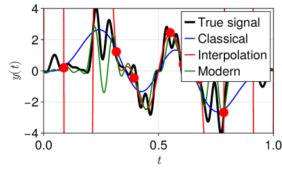
Figure 3: Aliasing occurs when basis functions that are independent over the entire domain are linearly dependent at the sampled points (left). When fitting a noisy signal (right), the classical sweet spot includes the dominant modes in the signal (blue). Over-fitting occurs when the combined contribution from the unmodeled modes is aliased into the model parameters, producing wild swings in the model predictions (red). Including additional terms allows the learning algorithm to distribute that signal over several basis terms. The result is a model whose predictions oscillate rapidly on a scale that is statistically similar to the true signal (green).

This mathematical derivation is represented visually in the left panel of Fig. 3: although basis functions are independent over the entire prediction domain, they may make identical predictions over the sampled subset (red dots). If the true signal contains contributions from all basis functions, but only a subset is explicitly modeled, the contribution from the unmodeled modes is aliased into the truncated representation.

The right panel shows three fits for an artificial data set using the Fourier basis. The true signal (black) includes contributions from all Fourier modes (although the low-frequency modes dominate). The classical sweet spot (blue) only models the dominant modes and produces a reasonable interpolation. At the interpolation threshold (red), however, the aliasing operator magnifies the unmodeled modes, producing large swings in the model predictions between the training samples. Beyond the interpolation threshold (green), the additional, high-frequency basis elements temper the aliasing effects by redistributing the signal among multiple basis functions. The result is a rapidly oscillating signal that does not exhibit the wild swings of overfitting. Although the oscillations in this inferred signal do not match those of the true signal, they are statistically similar, leading to reasonable model predictions.

II.4 Real-World Example: Cluster Expansion

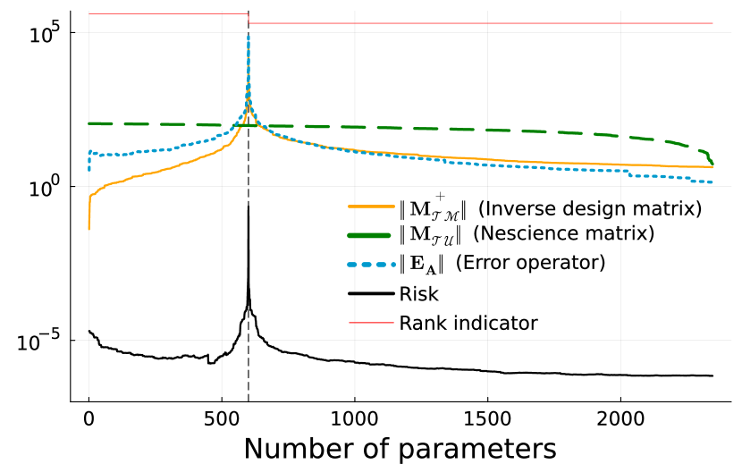
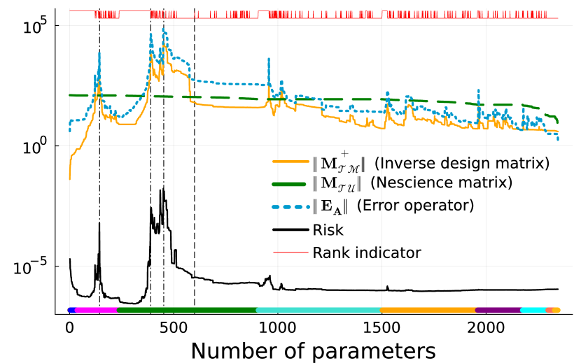
Figure 4: Norm of the operators and true risk of the cluster expansion model of Section II.4 as model complexity is increased (i.e., as parameters are added) with 600 training points. The interpolation threshold is indicated by a vertical dashed line. The red curve at the top of each panel is an indicator function which is high when the added basis function is linearly independent and low when it is linearly dependent. (Left) Rows and columns of $\mathbf{M}$ have been randomly ordered. (Right) Multiple peaks and valleys occur (indicated by dash-dot vertical lines) when the rows and columns of the design matrix are given by a “physical” ordering. The colors on the $x$-axis indicate “vertex order” (see text) of the atomic interactions: blue$\rightarrow$pairwise, magenta$\rightarrow$three-body, green$\rightarrow$four-body, etc.

Finally, we consider a model frequently used in high-throughput materials discovery. The cluster expansion model is a generalized Ising model [34, 35, 36, 37, 38, 39, 40, 41, 42] that in typical applications has hundreds to thousands of data points and a dozen to hundreds of inferred parameters. The prototypical application of the cluster expansion is predicting the energy $E$ of an alloy as a function of elemental composition and configuration $\vec{\sigma}$.

$$E(\vec{\sigma})=J_{0}+\sum_{i}J_{1}\xi_{i}+\sum_{i,j}J_{2}\xi_{i}\xi_{j}+\sum_{i,j,k}J_{3}\xi_{i}\xi_{j}\xi_{k}\\ +\sum_{i,j,k,l}J_{4}\xi_{i}\xi_{j}\xi_{k}\xi_{l}+\cdots,$$ (46)

where the indices run over all the possible sites, pairs of sites, triples, and so on. The $J$’s are expansion coefficients (inferred parameters, analogous to the $\theta$’s in the notation above). The products of $\xi(\vec{\sigma})$ functions form an orthogonal basis in the discrete vector space of all possible atomic configurations. This model has a physically intuitive interpretation. A product of two functions, $\xi_{i}\xi_{j}$, represents a pairwise interaction between atoms on sites $i$ and $j$. The sign of $J_{ij}$ determines whether like or unlike atoms prefer to be ${ij}$-neighbors.

One can enumerate all possible configurations (up to some maximum number of atoms)[44, 45, 46] and determine a complete set of basis functions[35]. Choosing a realistic model size, we explain the resulting generalization curve through the lens of generalized aliasing. A binary alloy model containing up to ten unique atomic sites has 2346 unique configurations. Figure 4 shows the norms of the aliasing, nescience, and invertability operators as a function of increasing basis size for a fixed number of training points.

We first consider the case where there is no natural ordering to either the data or parameters by randomizing rows and columns of $\mathbf{M}$, in line with the unstructured model ansatz above. The resulting behavior (left panel of Fig. 4) aligns with most presentations of double descent in the literature. Before the interpolation threshold, the behavior of the risk curve is the expected U-shape of the classical bias/variance trade-off. Beyond the interpolation threshold, the norms drop, consistent with the generalized aliasing analysis. Furthermore, the optimal model is not at the classical sweet spot but in the asymptotic modern regime since there is little over-modeling.

Like many modeling problems, practitioners have some intuition about the natural order for the sample points and basis functions. In the typical preferred ordering for cluster expansion, pair-wise interactions precede triplet interactions, and all triplet interactions come before any quadruplets, and so forth (reflected in the coloring of the $x$-axis in the right panel of Fig. 4). Furthermore, the terms are ordered in each class by diameter—short pairs before long pairs, small diameter triplets before extended triplets, etc. This ordering is motivated by physical arguments that the strongest interactions are short-range and low-body. For the ordering of the sample points (atomic configurations, rows of $\mathbf{M}$), there is the coarse guideline of ordering by “size,” denoted by the number of atoms in each configuration, but within each size class a natural ordering is not obvious.

For the right panel of Fig. 4, this $n$-body/short-long ordering was used to arrange columns and rows in $\mathbf{M}$. In addition to the complex behavior of the operator norms, note that the peak of the generalization error is not at the naive interpolation threshold where the number of parameters is equal to the number of training points. In fact, the interpolation threshold appears to not play a significant role in the generalization curve.

The norms show a complicated behavior, neither the typical U-shape of classical bias–variance trade-off nor the basic double descent. Rather, the generalization curve has multiple peaks and valleys, whose positions correspond to locations where added basis functions transition from linear independence to linear dependence (red “indicator function”).

Why do the norms of the different parts of the decomposition have this complicated structure? The answer is structure introduced by the physical ordering of the rows and columns of the design matrix. As shown by the red indicator function near the top of the right panel, basis functions that increase the rank of the design matrix $\mathbf{M}_{\mathcal{T}\mathcal{M}}$ increase the norm of its pseudoinverse and of the aliasing matrix $\mathbf{A}$. Note the relationship between the indicator function (red) and the norms in the lower panel of Fig. 4.

Finally, we ask how well the aliasing decomposition explains the actual risk, indicated by the black-colored curves in Fig. 4 In the right panel, vertical dash-dot lines are included to clarify the connection between peaks in the operator norms $\|\mathbf{M}_{\mathcal{T}\mathcal{M}}^{+}\|$ and $\|\mathbf{A}\|$ (orange and blue) and peaks in the risk (solid black).

The complicated generalization curve is inconsistent with either the classical bias–variance trade-off or other explanations of double descent. In contrast, the close relationship between peaks in the risk (prediction error) and peaks in the norm of $\mathbf{M}_{\mathcal{T}\mathcal{M}}^{+}$ is striking. In the left panel, the only peak in the norms, and in the risk, is at the interpolation threshold. This behavior for the randomized case is much easier to rationalize, but the risk (prediction error) is much higher than for the naturally ordered case in the right panel. By preferentially ordering according to the physically dominant terms, the contribution to the signal from the nescience matrix $\mathbf{M}_{\mathcal{T}\mathcal{U}}\bm{\theta}_{\mathcal{U}}$ is small, scaling down the aliasing effects. Furthermore, for large models, the physical ordering exhibits asymptotic over-modeling, so that the optimal risk occuring at the classical “sweet-spot.”

III Discussion

The preceding formal analysis and examples of the generalized aliasing decomposition give practical, intuitive guidance for formulating models.

III.1 General Insights into Modeling

III.1.1 Choosing the Basis

If the $n$ training points are known and fixed, a modeler can control the norm of $\mathbf{M}_{\mathcal{T}\mathcal{M}}^{+}$ and $\mathbf{A}$ (and hence generically control the magnitude of the risk) by strategically choosing the basis functions, without knowing anything about the labels $\bm{y}$.

For example, consider what happens when we choose the first $n$ basis functions $\phi_{k}$ so that, when evaluated at the points $\bm{t}_{1},\dots,\bm{t}_{n}$, the resulting vectors $\bm{\varphi}_{k}=(\phi_{k}(\bm{t}_{1}),\dots,\phi_{k}(\bm{t}_{n}))$ are orthonormal. If the columns of $\mathbf{M}_{\mathcal{T}\mathcal{M}}$ are the first $m\leq n$ of these vectors, then the inverse $\mathbf{M}_{\mathcal{T}\mathcal{M}}^{+}$ has induced norm $\|\mathbf{M}_{\mathcal{T}\mathcal{M}}^{+}\|=1$. In this situation the norm is constant as $m$ increases up to $n$; and then for $m>n$, no matter which additional columns are added, the norm $\|\mathbf{M}_{\mathcal{T}\mathcal{M}}^{+}\|$ cannot increase and will eventually shrink to $0$ (almost surely). Thus, the product $\|\mathbf{M}_{\mathcal{T}\mathcal{M}}^{+}\|\|\mathbf{M}_{\mathcal{T}\mathcal{U}}\|$ in the upper bound

$$\|\mathbf{A}\|\leq\|\mathbf{M}_{\mathcal{T}\mathcal{M}}^{+}\|\|\mathbf{M}_{\mathcal{T}\mathcal{U}}\|$$

on the norm of $\mathbf{A}$ also can never increase with $m$, and we expect there to be no peak in $\|\mathbf{E}_{\mathbf{A}}\bm{\theta}\|$ at all—only descent.

In the discrete Fourier series example (Section II.II.3), the norm of $\mathbf{A}$ is always $1$ and does not decrease to $0$ because the columns of $\mathcal{M}$ are specially tuned to the training set to make $\mathbf{M}_{\mathcal{T}\mathcal{U}}$ consist of infinitely many copies of $\mathbf{M}_{\mathcal{T}\mathcal{M}}$. This aligning of the basis functions to sample points explains why extreme over-fitting is rarely a problem in discrete Fourier transforms, in spite of it being formally equivalent to ordinary least squares regression at the interpolation threshold.

III.1.2 Choosing Training Points

If the basis functions are given and fixed, but the modeler has some control over the choice of the training points, then they can control the norm $\|\mathbf{A}\|$ by strategically choosing the points $\bm{t}_{1},\dots,\bm{t}_{n}$. Again, this requires no knowledge of the labels $\bm{y}$.

For example, consider the case of fitting polynomial functions on the interval $[-1,1]$ with the Legendre basis. For a given number $m$ of model parameters (the first $m$ Legendre polynomials), if we are able to choose $n$ points at which to evaluate the basis functions, then choosing the points to be the $n$ Legendre–Gauss points, which are the zeros of $P_{n}$, gives much better results than choosing the points randomly (drawn uniformly). This is shown in Figure 5, where the randomly chosen training points make $\|\mathbf{E}_{\mathbf{A}}\|$ many orders of magnitude larger than with the specially chosen Legendre–Gauss points. In this case a judicious choice of training points makes a huge difference.

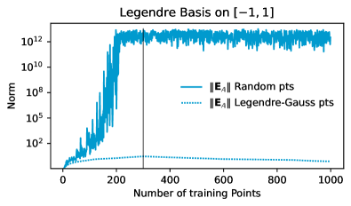
Figure 5: The induced norm of $\mathbf{E}_{\mathbf{A}}$ for the Legendre basis with the model consisting of the first $m=300$ Legendre polynomials. The norms are plotted as functions of the number $n$ of training points, and the vertical black line indicates the interpolation threshold. The solid line shows the result when the training points are chosen randomly (drawn uniformly from $[-1,1]$), while the dotted line shows the results when the $n$ training points are chosen to be the Legendre–Gauss points (the zeros of the $n$th Legendre polynomial). The norm of $\mathbf{A}$ is many orders of magnitude larger for randomly chosen training points than for the Legendre–Gauss points.

III.1.3 Conditioning of $\mathbf{M}$

If $\mathbf{M}$ is poorly conditioned, then it is possible to have a relatively small error $\mathbf{E}_{\bm{\theta}}\bm{\theta}$ in the parameters that corresponds to a large error in the signal. Thus it is desirable to select a basis that makes the full transformation $\mathbf{M}$ well conditioned.

For polynomial approximation with the standard monomial basis $\{1,t,t^{2},\dots\}$, the transformation $\mathbf{M}$ is a generalized Vandermonde matrix, which is very badly conditioned and generally should not be used with real-valued inputs. But polynomial approximation for real inputs in the interval $[-1,1]$ is well conditioned with the Chebyshev polynomial basis or the Legendre polynomial basis.

III.2 Regularization

It has been observed that $L^{2}$-regularization (ridge regression) generally reduces the size of the peak in risk at the interpolation threshold, but it can also increase bias [32, 50, 51]. This can be understood in terms of the impact of regularization on the pseudoinverse design matrix.

For a given decomposition of the space $\Theta=\mathcal{M}\oplus\mathcal{U}$ with $m=\dim\mathcal{M}$ model parameters, ridge regression amounts to changing the objective from minimizing risk to minimizing

$$\frac{1}{n}\|\bm{y}-\mathbf{M}_{\mathcal{T}\mathcal{M}}\bm{\theta}_{\mathcal{M}}\|_{2}^{2}+\lambda\|\bm{\theta}_{\mathcal{M}}\|_{2}^{2},$$ (47)

where $n$ is the the number of training points and $\lambda$ is a user-chosen parameter. As shown in Section IV.IV.4, this is equivalent to the alternative problem of minimizing

$$\left\|\widetilde{\bm{y}}-\widetilde{\mathbf{M}}_{\mathcal{T}\mathcal{M}}\bm{\theta}_{\mathcal{M}}\right\|_{2}^{2},$$

where $\widetilde{\bm{y}}=(\bm{y},\bm{0})$ and the smallest singluar value of $\widetilde{\mathbf{M}}_{\mathcal{T}\mathcal{M}}$ is at least ${\sqrt{n\lambda}}$. That means the norm of the pseudoinverse satisfies

$$\|\widetilde{\mathbf{M}}_{\mathcal{T}\mathcal{M}}^{+}\|\leq\frac{1}{\sqrt{n\lambda}}.$$

This bound is independent of both $m$ and $\mathbf{M}_{\mathcal{T}\mathcal{M}}$, and it essentially removes the impact of any small singular values of $\mathbf{M}_{\mathcal{T}\mathcal{M}}$ on the norms of $\mathbf{M}_{\mathcal{T}\mathcal{M}}^{+}$ and $\mathbf{A}$. This explains why there is no significant peak in the risk at the interpolation threshold (or anywhere else, for that matter) for $L_{2}$-regularized (ridge regression) problems, provided $\lambda$ is sufficiently large.

If $\sqrt{n\lambda}>\|\mathbf{M}_{\mathcal{T}\mathcal{U}}\|$, then the norm of $\mathbf{A}$ is smaller than the norm of $\mathbf{E}_{\mathbf{B}}$, so risk is always dominated by invertibility error $\mathbf{E}_{\mathbf{B}}\bm{\theta}$.

The invertibility error, however, can increase with regularization because the model bias term is no longer the projection of $\bm{\theta}_{\mathcal{M}}$ onto the null space $\mathcal{N}$ of $\mathbf{M}_{\mathcal{T}\mathcal{M}}$ but instead is $\|(\mathbf{I}_{\mathcal{M}}-\widetilde{\mathbf{M}}_{\mathcal{T}\mathcal{M}}^{+}\mathbf{M}_{\mathcal{T}\mathcal{M}})\bm{\theta}_{\mathcal{M}}\|$. When $\lambda$ is large, the fact that $\|\widetilde{\mathbf{M}}_{\mathcal{T}\mathcal{M}}^{+}\mathbf{M}_{\mathcal{T}\mathcal{M}}\|\leq\frac{\|\mathbf{M}_{\mathcal{T}\mathcal{M}}\|}{\sqrt{n\lambda}}$, means that the model bias term approaches $\|\bm{\theta}_{\mathcal{M}}\|$, which is generally larger than the projection $\|\mathbf{P}_{\mathcal{N}}\bm{\theta}_{\mathcal{M}}\|$. Nevertheless, the norm of $\mathbf{E}_{\mathbf{B}}$, while no longer necessarily bounded by $1$, is still bounded by

$$\|\mathbf{E}_{\mathbf{B}}\|\leq 1+\frac{\|\mathbf{M}_{\mathcal{T}\mathcal{M}}\|}{\sqrt{n\lambda}}.$$

III.3 Outlook

Successful model building involves numerous technical decisions related to the selection of model class, experimental design, learning algorithm, regularization, and other factors that can strongly impact the model’s predictive performance. Best practices are more often art, tuned to experience, rather than science guided by formal reasoning. The generalized aliasing decomposition (34) facilitates reasoning about key modeling decisions in a way that is both formal and intuitive. In the context of linear regression, the approach is fully rigorous while imbuing practitioners with intuition about model performance in both the classical and modern regimes. Because it gives a label-independent decomposition of risk, practitioners can also make informed choices about data collection and experimental design for target applications.

Although our formal analysis has been restricted to linear regression, there are reasons to be optimistic that the core approach generalizes to the nonlinear regime. First, the concepts of aliasing and invertibility extend formally to nonlinear operators and can be approximated through local linearization. Furthermore, many cases of practical importance may be tractable in the present framework. Neural tangent kernel techniques, for example, demonstrate that wide networks are linear in their models throughout training[52]. In addition, information geometry techniques applied to large, “sloppy” models have shown that most nonlinearity is “parameter-effects” and removable, in principle, through an appropriate, nonlinear reparameterization[53].

An important open question is: Under what conditions is the asymptotic risk less than that of the classical “sweet spot”? The preceding analysis has sharpened that question to: When will there be over-modeling? Random feature models, such as in Figure 2, but presumably also neural networks and other machine learning models, are approximately unstructured, so they do not exhibit over-modeling and are generically most effective in the over-parameterized, modern regime. In contrast, physics-based models are most effective in the classical regime, where they leverage prior knowledge.

Framing the question in this way clarifies why classical statistics historically missed these interesting phenomena, in spite of the essential elements being known to diverse communities for decades [10]. It also apparently partitions predictive modeling into two philosophically distinct camps: physical models using classical statistics and unstructured models in the modern, interpolating regime. In our cluster expansion example, the former approach gave the model with the least risk. Although perhaps expected, as physics-based modeling leverages prior information, this benefit comes after considerable effort from the materials science community. However, it remains unclear if these are inherently irreconcilable philosophies or two points on a broad landscape just beginning to be explored.

Indeed, our work demonstrates how the theoretical and technical challenges posed by modern data science overlap with those in other fields, including signal processing, control theory, and statistical physics. We hope that the perspectives advanced here will inspire theorists and practitioners alike to better understand and leverage the relationship between data science and the broader scientific milieu.

IV Methods

In this section we give the mathematical details of our explanation of the nonmonotonic curve occurring for the operator norm $\|\mathbf{A}\|$ (including the presence of ‘double descent’), both the peak at the interpolation threshold and the long-term decay to $0$ as the number of model parameters grows to $\infty$. We also prove the described results about $\|\mathbf{E}_{\mathbf{B}}\|$ and $L^{2}$-regularization.

IV.1 Interleaving of Eigenvalues in Rank-one Updates

The main tool we use to place the ideas presented in this paper on a rigorous footing is the following theorem, whose earliest statement seems to be [54, Theorem 17] (see also [55, 56, 57]).

Theorem IV.1.

Let $A$ be an $n\times n$ Hermitian matrix with eigenvalues $\alpha_{1}\geq\alpha_{2}\geq\cdots\geq\alpha_{n}$ and let $C$ be a positive semidefinite matrix of rank $1$. The eigenvalues $\beta_{1}\geq\beta_{2}\geq\cdots\geq\beta_{n}$ of the matrix $B=A+C$ satisfy

$$\beta_{1}\geq\alpha_{1}\geq\beta_{2}\geq\alpha_{2}\geq\cdots\geq\beta_{n}\geq\alpha_{n}.$$

From this theorem we immediately deduce the corollary that, under the same assumptions on $A$ and $C$, the eigenvalues $\delta_{1}\geq\cdots\geq\delta_{n}$ of $D=A-C$ are below the corresponding eigenvalues of $A$ and interleaved:

$$\alpha_{1}\geq\delta_{1}\geq\alpha_{2}\geq\cdots\geq\alpha_{n}\geq\delta_{n}.$$

Theorem IV.1 also leads us to the following fundamental result for analyzing the operator norms of the aliasing and invertibility operators $\mathbf{A}$ and $\mathbf{B}$ at least in the finite dimensional case.

Theorem IV.2.

Let $\mathbf{X}$ be an $m\times n$ matrix of rank $r$ with smallest singluar value $\sigma_{r}>0$. Let $\widetilde{\mathbf{X}}=[\mathbf{X}|\bm{\varphi}]$ be the $m\times(n+1)$ matrix obtained by adjoining an $m$-dimensional column vector $\bm{\varphi}$ to $\mathbf{X}$. The smallest singular value $\widetilde{\sigma}_{min}>0$ of $\widetilde{\mathbf{X}}$ satisfies the following relations:

$$0 <\widetilde{\sigma}_{min}\leq\sigma_{r} \operatorname{rank}(\mathbf{X})<\operatorname{rank}(\widetilde{\mathbf{X}})$$ if ,

$$0 <{\sigma}_{r}\leq\widetilde{\sigma}_{min} \operatorname{rank}(\mathbf{X})=\operatorname{rank}(\widetilde{\mathbf{X}})$$ if .

Proof.

Both $\mathbf{X}\mathbf{X}^{\mathsf{T}}$ and $\widetilde{\mathbf{X}}\widetilde{\mathbf{X}}^{\mathsf{T}}$ are $m\times m$ positive definite Hermitian matrices. The singular value decomposition of $\mathbf{X}$ shows that the singular values $\sigma_{1}\geq\cdots\geq\sigma_{r}>0$ and the eigenvalues $\lambda_{1}\geq\cdots\geq\lambda_{m}$ of $\mathbf{X}\mathbf{X}^{\mathsf{T}}$ satisfy

$$\lambda_{1}=\sigma^{2}_{1}\geq\lambda_{2}=\sigma^{2}_{1}\geq\cdots\geq\lambda_{r}=\sigma^{2}_{r}>0=\lambda_{r+1}.$$

Similarly, the singular values $\widetilde{\sigma}_{1}\geq\widetilde{\sigma}_{2}\geq\cdots$ and eigenvalues $\widetilde{\lambda}_{1}\geq\cdots\geq\widetilde{\lambda}_{m}$ of $\widetilde{\mathbf{X}}\widetilde{\mathbf{X}}^{\mathsf{T}}$ satisfy

$$\widetilde{\lambda}_{1}=\widetilde{\sigma}^{2}_{1}\geq\widetilde{\lambda}_{2}=\widetilde{\sigma}^{2}_{2}\cdots\geq\widetilde{\lambda}_{r}=\widetilde{\sigma}^{2}_{r}\geq\widetilde{\lambda}_{r+1}\geq\cdots,$$

where $\widetilde{\lambda}_{r+1}=0$ if $\operatorname{rank}(\widetilde{\mathbf{X}})=r$, but $\widetilde{\lambda}_{r+1}>0$ if $\operatorname{rank}(\widetilde{\mathbf{X}})=r+1$.

Expanding $\widetilde{\mathbf{X}}\widetilde{\mathbf{X}}^{\mathsf{T}}$ gives $\widetilde{\mathbf{X}}\widetilde{\mathbf{X}}^{\mathsf{T}}=\mathbf{X}\mathbf{X}^{\mathsf{T}}+\bm{\varphi}\bm{\varphi}^{\mathsf{T}}$, where $\bm{\varphi}\bm{\varphi}^{\mathsf{T}}$ is positive semidefinite, so Theorem IV.1 implies that

$$\widetilde{\lambda}_{1}\geq\lambda_{1}\cdots\geq\lambda_{r-1}\geq\widetilde{\lambda}_{r}\geq\lambda_{r}\geq\widetilde{\lambda}_{r+1}\geq 0.$$

If $\operatorname{rank}(\widetilde{\mathbf{X}})=r+1$ (that is, $\bm{\varphi}$ is not in the column space of $\mathbf{X}$), then $\lambda_{r}=\sigma^{2}_{r}\geq\widetilde{\lambda}_{r+1}=\widetilde{\sigma}^{2}_{r+1}>0$. Taking square roots gives $\sigma_{r}>\widetilde{\sigma}_{r+1}=\widetilde{\sigma}_{min}>0$.

If $\operatorname{rank}(\widetilde{\mathbf{X}})=r$ (that is, $\bm{\varphi}$ is in the column space of $\mathbf{X}$), then the smallest nonzero eigenvalue of $\widetilde{\mathbf{X}}\widetilde{\mathbf{X}}^{\mathsf{T}}$ is $\widetilde{\lambda}_{r}$, which satisfies $\lambda_{r-1}\geq\widetilde{\lambda}_{r}\geq\lambda_{r}>0$. Taking square roots gives $\widetilde{\sigma}_{min}=\widetilde{\sigma}_{r}\geq\sigma_{r}>0$, as required. ∎

IV.2 Norm of $\mathbf{A}$

We are interested in how the (induced) operator norm

$$\|\mathbf{A}\|=\|\mathbf{M}_{\mathcal{T}\mathcal{M}}^{+}\mathbf{M}_{\mathcal{T}\mathcal{U}}\|\leq\|\mathbf{M}_{\mathcal{T}\mathcal{M}}^{+}\|\|\mathbf{M}_{\mathcal{T}\mathcal{U}}\|$$

changes as the model grows, that is, as a new column is removed from $\mathbf{M}_{\mathcal{T}\mathcal{U}}$ and added to $\mathbf{M}_{\mathcal{T}\mathcal{M}}$, but the training set (which rows are included) remains unchanged.

For simplicity of notation and to make the dependence on the number $m$ of model parameters explicit we write $\mathbf{X}(m)=\mathbf{M}_{\mathcal{T}\mathcal{M}}$ and $\mathbf{Y}(m)=\mathbf{M}_{\mathcal{T}\mathcal{U}}$ when the model consists of the first $m$ columns of $\mathbf{M}$. The matrix $\mathbf{X}(m+1)$ is constructed by moving one column $\bm{\varphi}_{m+1}$ from $\mathbf{M}_{\mathcal{T}\mathcal{U}}$ to $\mathbf{M}_{\mathcal{T}\mathcal{M}}$ and the projection of the operator $\mathbf{M}$ onto the training space $\mathcal{T}$ decomposes as $\begin{bmatrix}\mathbf{X}(m)&\bm{\varphi}_{m+1}&\mathbf{Y}(m+1)\end{bmatrix}$.

IV.2.1 Nescience:

First consider what happens to the nescience matrix $\mathbf{M}_{\mathcal{T}\mathcal{U}}$ when a column $\bm{\varphi}_{m+1}$ is removed from $\mathbf{Y}(m)=[\bm{\varphi}_{m}\quad\mathbf{Y}(m+1)]$. Expanding the product $\mathbf{Y}(m)\mathbf{Y}(m)^{\mathsf{T}}$ gives $\mathbf{Y}(m)\mathbf{Y}(m)^{\mathsf{T}}=\bm{\varphi}_{m+1}\bm{\varphi}_{m+1}^{\mathsf{T}}+\mathbf{Y}(m+1)\mathbf{Y}(m+1)^{\mathsf{T}}$. Since $\bm{\varphi}_{m+1}\bm{\varphi}_{m+1}^{\mathsf{T}}$ is positive semidefinite, Theorem IV.1 applies and guarantees that the norms satisfy $\|\mathbf{Y}(m)\|\geq\|\mathbf{Y}(m+1)\|$, and thus the norm $\|\mathbf{Y}(m)\|$ is a nonincreasing function of $m$.

IV.2.2 Pseudoinverse of Design:

Consider now the pseudoinverse term $\|\mathbf{M}_{\mathcal{T}\mathcal{M}}^{+}\|$ when $\bm{\varphi}_{m+1}$ is adjoind to $\mathbf{X}(m)$ to create $\mathbf{X}(m+1)$. Theorem IV.2 guarantees that whenever $\bm{\varphi}_{m+1}$ is linearly independent of the old model (does not lie in the column space of $\mathbf{X}(m)$), then the induced norm of the new pseudoinverse is bounded below by the induced norm of the old pseudoinverse:

$$\|\mathbf{X}(m+1)^{+}\|\geq\|\mathbf{X}(m)^{+}\|.$$

Similarly, when $\bm{\varphi}_{m+1}$ is linearly dependent on the old model, then the induced norm of the new pseudoinverse is bounded above by the norm of the previous pseudoinverse

$$\|\mathbf{X}(m+1)^{+}\|_{2}\leq\|\mathbf{X}(m)^{+}\|_{2}.$$

This proves Theorem II.1.

IV.2.3 Limiting behavior of $\mathbf{A}$

As the number $m$ of model parameters gets large, the norm $\|\mathbf{A}\|$ is dominated by the norm of the pseudoinverse $\|\mathbf{M}_{\mathcal{T}\mathcal{M}}^{+}\|$. For purposes of this analysis, assume that the columns of $\mathbf{M}_{\mathcal{T}\mathcal{M}}$ are independent identically distributed (i.i.d.) random vectors $\bm{\varphi}_{i}\in\mathbb{R}^{n}$ with (finite) second moment $\mathbb{E}[\bm{\varphi}_{i}\bm{\varphi}_{i}^{\mathsf{T}}]=\Sigma$, where $\Sigma$ is of full rank (rank $t$).

The Strong Law of Large Numbers guarantees that

$$\frac{1}{m}\mathbf{X}(m)\mathbf{X}(m)^{\mathsf{T}}=\frac{1}{m}\sum_{i=1}^{m}\bm{\varphi}_{i}\bm{\varphi}_{i}^{\mathsf{T}}\stackrel{{\scriptstyle a.s.}}{{\longrightarrow}}\mathbb{E}[\bm{\varphi}_{i}\bm{\varphi}_{i}^{\mathsf{T}}]=\Sigma$$

as $m\to\infty$. This implies that the smallest singular value of $\frac{1}{m}\mathbf{X}(m)\mathbf{X}(m)^{\mathsf{T}}$ converges almost surely to the smallest singular value of $\Sigma$, and thus the smallest singular value $\lambda_{min}(m)$ of $\mathbf{X}(m)\mathbf{X}(m)^{\mathsf{T}}$ goes to infinity almost surely. Thus the smallest singular value $\sigma_{min}(m)=\sqrt{\lambda_{min}(m)}$ of $\mathbf{X}(m)$ also goes to infinity, and this implies $\|\mathbf{X}(m)^{+}\|=\frac{1}{\sigma_{min}}\stackrel{{\scriptstyle a.s.}}{{\longrightarrow}}0$.

Because $\|\mathbf{Y}(m)\|=\|\mathbf{M}_{\mathcal{T}\mathcal{U}}\|$ is bounded above and decreasing in $m$, we have

$$\|\mathbf{A}(m)\|=\|\mathbf{X}(m)^{+}\mathbf{Y}(m)\|\leq\|\mathbf{X}(m)^{+}\|\|\mathbf{Y}(m)\|\stackrel{{\scriptstyle a.s.}}{{\longrightarrow}}0.$$

In the special case that the vectors $\bm{\varphi}_{i}$ are i.i.d. standard normal and $m>n$, it is known [58, Thm 2.6] that $\mathbb{E}[\sigma_{min}(m)]\geq\sqrt{m}-\sqrt{n}$, so $\|\mathbf{X}(m)^{+}\|$ and $\mathbf{A}(m)$ are $O(m^{-1/2})$ or smaller.

IV.3 Norm of $\mathbf{E}_{\mathbf{B}}$ and $\mathbf{E}_{\mathbf{B}}\bm{\theta}$

Let $\mathbf{M}_{\mathcal{T}\mathcal{M}}=U_{1}\Sigma_{1}V_{1}^{\mathsf{T}}$ be the reduced SVD of $\mathbf{M}_{\mathcal{T}\mathcal{M}}$, where $\mathbf{M}_{\mathcal{T}\mathcal{M}}$ has rank $r$ and $\Sigma_{1}$ is invertible of shape $r\times r$. This gives

$$\mathbf{B}=\mathbf{M}_{\mathcal{T}\mathcal{M}}^{+}\mathbf{M}_{\mathcal{T}\mathcal{M}}=V_{1}\Sigma_{1}^{-1}\Sigma_{1}V_{1}^{\mathsf{T}}=V_{1}V_{1}^{\mathsf{T}}.$$

The matrix $V_{1}$ consists of the first $r$ columns of an orthonormal matrix $V$, i.e., $V=[V_{1}|V_{2}]$, with $VV^{\mathsf{T}}=V_{1}V_{1}^{\mathsf{T}}+V_{2}V_{2}^{\mathsf{T}}=\mathbf{I}$. Hence Theorem IV.1 guarantees that

$$\|\mathbf{B}\| =\|V_{1}V_{1}^{\mathsf{T}}\|\leq\|\mathbf{I}\|=1$$

and

$$\|\mathbf{I}-\mathbf{B}\| =\|V_{2}V_{2}^{\mathsf{T}}\|\leq 1.$$

Note that $V_{2}V_{2}^{\mathsf{T}}=\mathbf{P}_{\mathcal{N}}$ is the projection onto the kernel $\mathcal{N}$ of $\mathbf{M}_{\mathcal{T}\mathcal{M}}$, and every projection operator has its norm bounded by $1$, so

$$\|\mathbf{E}_{\mathbf{B}}\|=\left\|\begin{pmatrix}\mathbf{P}_{\mathcal{N}}&0\\ 0&\mathbf{I}_{\mathcal{U}}\end{pmatrix}\right\|\leq 1,$$

and equality holds except in the rare and uninteresting case that the entire paramter space is modeled: $\Theta=\mathcal{M}$ and $\mathcal{U}=\{\bm{0}\}$. This also implies that $\|\mathbf{E}_{\mathbf{B}}\bm{\theta}\|\leq\|\bm{\theta}\|$.

As discussed in Section II.II.1.4, to better understand the dependence of $\mathbf{E}_{\mathbf{B}}\bm{\theta}$ on the model dimension $m$, we decompose the square of the norm $\|\mathbf{E}_{\mathbf{B}}\|^{2}$ further into model invertibility and nescience contributions

$$\|\mathbf{E}_{\mathbf{B}}\bm{\theta}\|^{2}=\|\mathbf{P}_{\mathcal{N}(m)}\bm{\theta}_{\mathcal{M}(m)}\|^{2}+\|\bm{\theta}_{\mathcal{U}(m)}\|^{2}$$ (48)

with explicit $m$-dependence. Model-invertibility is a nondecreasing function of $m$ because $\mathcal{N}(m)\subseteq\mathcal{N}(m+1)$ for all $m$. Similarly, $\mathcal{U}(m)\supseteq\mathcal{U}(m+1)$, so the nescience contribution is nonincreasing, and, indeed, it decreases by exactly $|\theta_{m+1}|^{2}$ when moving from $m$ to $m+1$.

IV.4 Regularization

It is straightforward to verify that the objective to minimize with $L_{2}$-regularization can be written as $\frac{1}{n}\left\|\widetilde{\bm{y}}-\widetilde{\mathbf{M}}_{\mathcal{T}\mathcal{M}}\bm{\theta}_{\mathcal{M}}\right\|_{2}^{2},$ where $\widetilde{\mathbf{M}}_{\mathcal{T}\mathcal{M}}=\left[\begin{smallmatrix}\mathbf{M}_{\mathcal{T}\mathcal{M}}\\ \sqrt{n\lambda}\mathbf{I}_{m}\end{smallmatrix}\right]$ and $\widetilde{\bm{y}}=\left[\begin{smallmatrix}\bm{y}\\ \bm{0}\end{smallmatrix}\right]$. This changes changes $\mathbf{E}_{\mathbf{B}}$ to $\begin{bmatrix}I_{\mathcal{M}}-\widetilde{\mathbf{M}}_{\mathcal{T}\mathcal{M}}^{+}\mathbf{M}_{\mathcal{T}\mathcal{M}}&0\\ 0&I_{\mathcal{U}}\end{bmatrix}$ and changes $\mathbf{A}$ to $\widetilde{\mathbf{M}}_{\mathcal{T}\mathcal{M}}^{+}\mathbf{M}_{\mathcal{T}\mathcal{U}}$. Expanding the product

$$\widetilde{\mathbf{M}}_{\mathcal{T}\mathcal{M}}\widetilde{\mathbf{M}}_{\mathcal{T}\mathcal{M}}^{\mathsf{T}}=\mathbf{M}_{\mathcal{T}\mathcal{M}}\mathbf{M}_{\mathcal{T}\mathcal{M}}^{\mathsf{T}}+n\lambda\mathbf{I}_{m},$$

shows that every eigenvalue of $\mathbf{M}_{\mathcal{T}\mathcal{M}}\mathbf{M}_{\mathcal{T}\mathcal{M}}^{\mathsf{T}}$ is now increased by $n\lambda$ in this product. Therefore, the singular values of $\mathbf{M}_{\mathcal{T}\mathcal{M}}$ are all increased by $\sqrt{n\lambda}$ in $\widetilde{\mathbf{M}}_{\mathcal{T}\mathcal{M}}$, and

$$\|\widetilde{\mathbf{M}}_{\mathcal{T}\mathcal{M}}^{+}\| =\frac{1}{\frac{1}{\|{\mathbf{M}_{\mathcal{T}\mathcal{M}}}^{+}\|}+\sqrt{n\lambda}}$$

$$=\frac{\|{\mathbf{M}_{\mathcal{T}\mathcal{M}}}^{+}\|}{1+\sqrt{n\lambda}\|{\mathbf{M}_{\mathcal{T}\mathcal{M}}}^{+}\|}\leq\frac{1}{\sqrt{n\lambda}}.$$